Fractal Functions, Dimensions and Signal Analysis Santo Banerjee
Fractal Functions, Dimensions and Signal Analysis Santo Banerjee
Fractal Functions, Dimensions and Signal Analysis Santo Banerjee
Fractal Functions, Dimensions and Signal Analysis Santo Banerjee
Fractal Functions, Dimensions and Signal Analysis Santo Banerjee
1.
Fractal Functions, Dimensionsand Signal
Analysis Santo Banerjee pdf download
https://textbookfull.com/product/fractal-functions-dimensions-
and-signal-analysis-santo-banerjee/
Download more ebook instantly today - get yours now at textbookfull.com
2.
We believe theseproducts will be a great fit for you. Click
the link to download now, or visit textbookfull.com
to discover even more!
Fractal Patterns in Nonlinear Dynamics and Applications
1st Edition Santo Banerjee (Author)
https://textbookfull.com/product/fractal-patterns-in-nonlinear-
dynamics-and-applications-1st-edition-santo-banerjee-author/
Fractal Functions, Fractal Surfaces, and Wavelets,
Second Edition Peter R. Massopust
https://textbookfull.com/product/fractal-functions-fractal-
surfaces-and-wavelets-second-edition-peter-r-massopust/
A Survey of Fractal Dimensions of Networks Eric
Rosenberg
https://textbookfull.com/product/a-survey-of-fractal-dimensions-
of-networks-eric-rosenberg/
Biota Grow 2C gather 2C cook Loucas
https://textbookfull.com/product/biota-grow-2c-gather-2c-cook-
loucas/
3.
Dirichlet Series andHolomorphic Functions in High
Dimensions (New Mathematical Monographs) 1st Edition
Andreas Defant
https://textbookfull.com/product/dirichlet-series-and-
holomorphic-functions-in-high-dimensions-new-mathematical-
monographs-1st-edition-andreas-defant/
Lifetime Analysis by Aging Intensity Functions
Magdalena Szymkowiak
https://textbookfull.com/product/lifetime-analysis-by-aging-
intensity-functions-magdalena-szymkowiak/
Measurement while drilling (MWD): signal analysis,
optimization, and design Chin
https://textbookfull.com/product/measurement-while-drilling-mwd-
signal-analysis-optimization-and-design-chin/
Quantum-Mechanical Signal Processing and Spectral
Analysis First Edition Belki■
https://textbookfull.com/product/quantum-mechanical-signal-
processing-and-spectral-analysis-first-edition-belkic/
Fractal Dimension for Fractal Structures: With
Applications to Finance Manuel Fernández-Martínez
https://textbookfull.com/product/fractal-dimension-for-fractal-
structures-with-applications-to-finance-manuel-fernandez-
martinez/
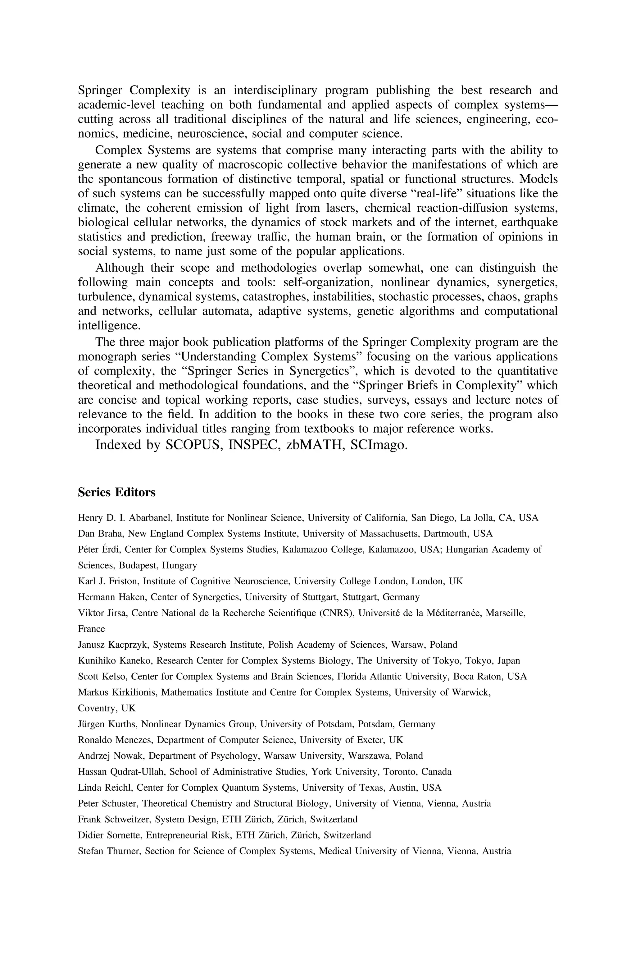
Springer Complexity isan interdisciplinary program publishing the best research and
academic-level teaching on both fundamental and applied aspects of complex systems—
cutting across all traditional disciplines of the natural and life sciences, engineering, eco-
nomics, medicine, neuroscience, social and computer science.
Complex Systems are systems that comprise many interacting parts with the ability to
generate a new quality of macroscopic collective behavior the manifestations of which are
the spontaneous formation of distinctive temporal, spatial or functional structures. Models
of such systems can be successfully mapped onto quite diverse “real-life” situations like the
climate, the coherent emission of light from lasers, chemical reaction-diffusion systems,
biological cellular networks, the dynamics of stock markets and of the internet, earthquake
statistics and prediction, freeway traffic, the human brain, or the formation of opinions in
social systems, to name just some of the popular applications.
Although their scope and methodologies overlap somewhat, one can distinguish the
following main concepts and tools: self-organization, nonlinear dynamics, synergetics,
turbulence, dynamical systems, catastrophes, instabilities, stochastic processes, chaos, graphs
and networks, cellular automata, adaptive systems, genetic algorithms and computational
intelligence.
The three major book publication platforms of the Springer Complexity program are the
monograph series “Understanding Complex Systems” focusing on the various applications
of complexity, the “Springer Series in Synergetics”, which is devoted to the quantitative
theoretical and methodological foundations, and the “Springer Briefs in Complexity” which
are concise and topical working reports, case studies, surveys, essays and lecture notes of
relevance to the field. In addition to the books in these two core series, the program also
incorporates individual titles ranging from textbooks to major reference works.
Indexed by SCOPUS, INSPEC, zbMATH, SCImago.
Series Editors
Henry D. I. Abarbanel, Institute for Nonlinear Science, University of California, San Diego, La Jolla, CA, USA
Dan Braha, New England Complex Systems Institute, University of Massachusetts, Dartmouth, USA
Péter Érdi, Center for Complex Systems Studies, Kalamazoo College, Kalamazoo, USA; Hungarian Academy of
Sciences, Budapest, Hungary
Karl J. Friston, Institute of Cognitive Neuroscience, University College London, London, UK
Hermann Haken, Center of Synergetics, University of Stuttgart, Stuttgart, Germany
Viktor Jirsa, Centre National de la Recherche Scientifique (CNRS), Université de la Méditerranée, Marseille,
France
Janusz Kacprzyk, Systems Research Institute, Polish Academy of Sciences, Warsaw, Poland
Kunihiko Kaneko, Research Center for Complex Systems Biology, The University of Tokyo, Tokyo, Japan
Scott Kelso, Center for Complex Systems and Brain Sciences, Florida Atlantic University, Boca Raton, USA
Markus Kirkilionis, Mathematics Institute and Centre for Complex Systems, University of Warwick,
Coventry, UK
Jürgen Kurths, Nonlinear Dynamics Group, University of Potsdam, Potsdam, Germany
Ronaldo Menezes, Department of Computer Science, University of Exeter, UK
Andrzej Nowak, Department of Psychology, Warsaw University, Warszawa, Poland
Hassan Qudrat-Ullah, School of Administrative Studies, York University, Toronto, Canada
Linda Reichl, Center for Complex Quantum Systems, University of Texas, Austin, USA
Peter Schuster, Theoretical Chemistry and Structural Biology, University of Vienna, Vienna, Austria
Frank Schweitzer, System Design, ETH Zürich, Zürich, Switzerland
Didier Sornette, Entrepreneurial Risk, ETH Zürich, Zürich, Switzerland
Stefan Thurner, Section for Science of Complex Systems, Medical University of Vienna, Vienna, Austria
6.
More information aboutthis series at http://www.springer.com/series/5394
Understanding Complex Systems
7.
Santo Banerjee •D. Easwaramoorthy •
A. Gowrisankar
Fractal Functions,
Dimensions and Signal
Analysis
123
Preface
The traditional interpolationtechniques generate smooth or piecewise differentiable
interpolation function, despite the data points being irregular. Nevertheless, most
of the natural objects such as lightning, clouds, mountain ranges, and wall cracks
have irregular and complex structures in which Euclidean geometry cannot be
applied successfully to describe them, since Euclidean geometry which deals with
regular objects and functions is used to approximate the data obtained from the
realistic environment. Hence, there is a need of a nonlinear tool in the approxi-
mation theory to resolve these problems. Barnsley invented the fractal interpolation
function based on the theory of iterated function systems, which precisely suited for
the approximation of naturally occurring functions which possess some kind of
self-similarity under magnification.
In the approximation theory, Fractal Interpolation Functions (FIF) play a vital
role. It is important and necessary to discuss the variance ratio of such functions.
But they are often nowhere differentiable, everywhere continuous. Hence, FIFs are
sophisticated in approximating the rough curve and precisely reconstructing the
naturally occurring functions when compared with classical interpolants.
Nevertheless, a smooth curve is needed to approximate some kind of functions
which include self-similarity under magnification. Hence, Barnsley presented the
indefinitely integrated fractal interpolation function generated from some special
type of the iterated function system which interpolates a certain set of data, and the
integral of the fractal interpolation function retains its properties. Further, they have
explored the construction of n-times frequently differentiable FIF when the
derivative values reaching up to the nth order are available at the initial endpoint
of the interval. The examples of differentiable functions cannot actually be con-
sidered as fractals, but they retain the name fractal interpolation function because
of the flavor of the scaling in the equation and the Hausdorff–Besicovitch dimen-
sion of their graphs are non-integer. Due to the sophisticated usage of such fractal
interpolants in nonlinear approximation, there are continuous efforts have extended
on fractal interpolation functions.
v
10.
As mentioned, theliterature and natural appearance of fractal functions moti-
vated us to write the book titled Fractal Functions, Dimensions and Signal Analysis
with the following facts. Initially, this book focuses on the construction of fractals
in a metric space through various iterated function systems. Chapter two discusses
the mathematical background behind the fractal interpolation functions and presents
its graphical representations. In chapters three, we appeal fractional integrals and
fractional derivatives on a linear fractal interpolation function. Further, the exis-
tence of a fractal interpolation function with a countable iterated function system is
demonstrated while taking xn as a monotone and bounded sequence, and yn as a
bounded sequence. Further, fractional order integral and integer-order integral of an
FIF for a sequence of data are described when the value of the integral of an FIF is
predefined at the initial endpoint or the final endpoint. Finally, the fractional
derivatives of an FIF and its fractional integrals are given due importance as they
are more precise and suitable for FIFs which are nowhere differentiable but con-
tinuous at all points. Hence, fractional calculus is a mathematical operator which
best suits for analyzing such an FIF and which may also change the fractal
dimension, when applied to fractal objects or functions.
As an application part, this book discusses the biomedical signal analysis in two
chapters. Chapter 5 concisely presents the overview of signal processing and its
mathematical background. Chapter 6 presents a wavelet-based denoising method
for the recovery of the Electroencephalogram (EEG) signal contaminated by
non-stationary noises and investigates the recognition of healthy and epileptic EEG
signals by using multifractal measures such as generalized fractal dimensions, since
the identification of abnormality in EEG signals is the vast area of research in
neuroscience. Especially, the classification of healthy and epileptic subjects through
EEG signals is a crucial problem in the biomedical sciences. Denoising of EEG
signals is another important task in signal processing. The noises must be corrected
or reduced before the subsequent decision analysis. Moreover, this chapter explores
the three different methods to explicitly recognize the healthy and epileptic EEG
signals: Modified, Improved, and Advanced forms of generalized fractal dimen-
sions. The newly proposed scheme is based on generalized fractal dimensions and
the discrete wavelet transform for analyzing the EEG signals.
Fractal functions have been covered with wavelet transformation and signals in
almost all the books published so far. This book for the first time emphasizes the
fractional calculus of fractal functions in various settings with applications of fractal
dimensions in biomedical signal analysis. We are delighted to welcome our readers
for a walkway in the domain of fractal functions, fractal dimensions, and their
manifestations in biomedical signals. This book has been composed with six sec-
tions which are organized as follows.
Chapter 1 starts with a broad outline of the iterated function system of con-
traction mappings. The Barnsley framework of IFS has been extended to the local
iterated function system and the countable iterated function system for constructing
the deterministic fractals, which is offered in Chap. 1. Consequently, the existence
of an attractor of the local countable iterated function system is investigated.
Moreover, it is proved that the local attractor of the local CIFS is expressed as the
vi Preface
11.
limit of aconvergence sequence of attractors of the local IFS. At the end of Chap. 1,
various notions of fractal dimensions are succinctly presented which will be applied
in the forthcoming chapters.
In Chap. 2, the concepts of fractal interpolation functions and their generaliza-
tions such as hidden variable fractal interpolation and a-fractal function are
described. The last part of the chapter is devoted to the traditional calculus theory,
an experienced tool that supports to implement the concept of spline approximation
to fractal functions.
In Chap. 3, the Riemann–Liouvllie fractional calculus of different types of fractal
interpolation functions is explored. The Riemann–Liouville fractional integral of
order b [ 0 of a quadratic fractal interpolation function with both constant and
variable scaling parameter is examined. In addition to that, the prominent influence
of free parameters in the shape of a fractal interpolation function is illustrated with
suitable examples.
In the traditional method of fractal interpolation and in practically the entirety of
its expansions referenced beforehand, a fractal interpolation function is constructed
for a finite data set. That is, the interpolation theory deals with the reconstruction of a
continuous function associated with the finite set of data ðxn; ynÞ : n ¼ 1; 2; . . .; N
f g.
Nevertheless, there are practical phenomena where infinite data points might be
justified, for example, in the theory of sampling and reconstruction. Recently, the
standard development of the univariate fractal interpolation function is reached out
from the finite case to the instance of a countable set of data. This development of a
fractal interpolation function for a prescribed countable set of data frames the reason
for the discussion of fractional calculus of a fractal interpolation function for
countable data in Chap. 4. However, Chap. 4 introduces and describes the sequence
of data and the corresponding interpolation function which is a generalization of the
Secelean framework. The existence of the continuous function f which interpolates
the sequence of prescribed data ðxn; ynÞ : n 2 N
f g is discussed, where ðxnÞ1
n¼1 is a
monotonic real sequence and ðynÞ1
n¼1 is a bounded sequence of real numbers.
Besides, the existence of a countable iterated function system is investigated when
the fractal interpolation function for a sequence of data is given. Further, the exis-
tence of the Riemann–Liouville fractional integral and the derivative of fractal
interpolation function is established.
In Chaps. 5 and 6, the designed multifractal methods were performed signifi-
cantly in the detection of epileptic seizures in EEG signals and ECG signals through
the cardiac inter-heartbeat time interval dynamics. The multifractal measures have
shown significant differences among normal, interictal, and ictal EEGs and dis-
criminate the young and elderly subjects by ECG inter-heartbeat signals. The
fuzzy-based multifractal theory for signals is established in order to define the fuzzy
generalized fractal dimensions by introducing the fuzzy membership function in the
classical generalized fractal dimensions method, and it is used for the classification
Preface vii
12.
of chaotic behaviorsin the fractal waveforms. In Chap. 6, a fuzzy multifractal
measure for biomedical signals to identify the age-group of subjects is presented.
Turin, Italy Santo Banerjee
Vellore, India D. Easwaramoorthy
Vellore, India A. Gowrisankar
viii Preface
2 1 MathematicalBackground of Deterministic Fractals
There has been a surge of research activities in applying the influential fractal
idea in pretty much every part of scientific disciplines to increase profound bits of
knowledge into numerous unresolved problems. However, there is no flawless and
complete definition of the fractal. The simplest way to define a fractal is as an object
which appears self-similar under varying degrees of magnification. A ‘Fractal’ is
generally a rough or fragmented geometric shape that can be split into parts, each of
which is (at least approximately) a reduced-size copy of the whole, a property called
self-similarity. The word Fractal is derived from the Latin word, fractus meaning
broken or fractured to describe objects that were too irregular to fit into a traditional
geometrical setting. In Mandelbrot’s original article, the Fractal is mathematically
defined as a set with the Hausdorff dimension strictly greater than its topological
dimension. Roughly speaking, a fractal set is a set that is more ‘irregular’ than the
sets considered in classical geometry. Fractal sets have the additional property of
being in some sense either strictly or statistically self-similar; this property has been
widely applied to model the numerous natural phenomena by Mandelbrot and oth-
ers. However, the notion of the strict self-similar property has been theoretically
framed by Hutchinson and popularized by Barnsley. The iterated function system is
a convenient and powerful way tool for generating fractals in a metric space with
specified self-similarity properties. Hutchinson introduced the conventional expla-
nation of deterministic fractals through the theory of Iterated Function System (IFS).
Meanwhile, Barnsley formulated the theory of IFS called the Hutchinson–Barnsley
(HB) theory in order to define and construct the fractals as a non-empty compact
invariant subset of a complete metric space which is generated by the Banach fixed
point theorem, known as IFS theory [2, 3]. In view of the applications of fractals to
comprehend the natural phenomena, every area of science has been concerned about
the fractal analysis. Hence, fractal analysis plays a central role in mathematics as a
tool for nonlinear applications and as a theory of interest.
Karl Weierstrass gave an example of a function with the non-intuitive property of
being everywhere continuous but nowhere differentiable, called Weierstrass Func-
tion, whose graph would today be considered as a fractal. The complexity and irreg-
ularity can be found in many physical and biological nonlinear systems naturally and
have been analyzed by the tools of fractal theory and computed by the non-integer or
fractional measure called Fractal Dimension. In approximation theory, the traditional
interpolation techniques generate a smooth or piecewise differentiable interpolation
function, despite the data points being irregular. Nevertheless, most of the natural
objects such as lightning, clouds, mountain ranges, and wall cracks have irregular
and complex structures in which Euclidean geometry cannot be applied successfully
to describe them. Hence, there is a need for a nonlinear tool in the approximation
theory to resolve these problems. M. F. Barnsley invented the Fractal Interpolation
Function (FIF) based on the theory of IFS, which precisely suited for the approxi-
mation of naturally occurring functions which possess some kind of self-similarity
under magnification [4]. Fractal interpolation functions are not necessarily differen-
tiable even though they are continuous everywhere. Hence, FIFs are sophisticated in
approximating the rough curve which precisely reconstructs the naturally occurring
functions when compared to the classical interpolants. Nevertheless, a smooth curve
17.
1.1 Introduction 3
isneeded to approximate some kind of functions which include the self-similarity
under magnification. Barnsley and Harrington explored the construction of p-times
frequently differentiable FIF when the derivative values reach up to pth order at the
initial endpoint of the interval [5].
During the past few years, numerous mathematical techniques were broadly cor-
related with fractal analysis. Considering the importance of fractional calculus for
discussing the variance ratio of fractal functions, the general relationship between
the fractional calculus and fractals has been investigated. Based on these studies,
there are continuous efforts connecting the fractional calculus, and the graphs of
the fractal function are available in the literature. Generally, the interpolation and
approximation of functions have been constructed by means of smooth functions,
often piecewise differentiable. However, the waves and signals from the real world
do not share this aspect. Hence, the main goal of the current book is to provide the
idea to approximate the rough (nowhere differentiable) functions through the fractal
interpolation function and its fractional calculus. Against this background, it is pro-
posed to generalize any interpolation function, smooth or rough, by means of a family
of fractal functions. It is also proposed to construct the various fractal interpolation
functions for a sequence of data and to investigate their shape-preserving properties.
Fractional calculus of such functions will be explored for approximating the rough
functions, additionally to correlate the fractional order and fractal dimension of the
fractal interpolation function.
The brain cells of humans start in between the 120th day and the 160th day of
pregnancy. It is accepted that from this beginning phase and throughout life, electri-
cal signals produced by the brain which speak to the cerebrum work as well as the
status of the entire body. In this direction, there are numerous advanced digital signal
processing methods applied on the biomedical signals, and thereby understand the
brain activity of a human. Signals from the human body play a vital role for the early
diagnosis of a variety of diseases. Such electrobiological signals can be in the form
of an electrocardiogram (ECG) taken from the heart, electromyogram (EMG) mea-
sured in muscles, electroencephalogram (EEG) from the brain, magnetoencephalo-
gram (MEG) given by the brain, electrogastrogram (EGG) from the stomach, and
electrooculogram (EOG) generated by eye nerves. As an application part, this book
discusses the signal analysis with respect to a multifractal perspective. Particularly,
fractal methods are applied on a medical signal, such as an Electroencephalogram
and Electrocardiogram, to help in the diagnosis. An EEG signal is a capacity of
currents that flow during synaptic excitations of the dendrites of many pyramidal
neurons in the cerebral cortex. The synaptic currents are formed within the dendrite
when neurons are activated. This current produces a magnetic field measurable by
electromyogram machines and a secondary electrical field over the scalp measurable
by EEG systems. There is ever-expanding worldwide interest for more moderate
and powerful clinical and medicinal services. New strategies and apparatus should
be created along these lines to help in the diagnosis, monitoring, and treatment of
abnormalities and diseases of the human body. Biomedical signs (biosignals) in their
complex structures are rich data sources, which when properly prepared can possibly
encourage such developments. In the present revolution, such preparing is probably
18.
4 1 MathematicalBackground of Deterministic Fractals
going to be digital, as affirmed by the incorporation of computerized signal handling
ideas as center preparing in biomedical science degrees. Ongoing developments in
digital signal preparing are relied upon to support key parts of things to come progress
in biomedical exploration and innovation, and the reason for this book is to feature
this pattern for the handling of estimations of brain activity, essentially electroen-
cephalograms. Similarly, Electrocardiogram is the vital sign most commonly used in
the clinical environment. It provides an insight into the understanding of many age-
related cardiac disorders. The vast existing literature on automatic ECG classification
comprises lot more methods based on pattern recognition methodologies, artificial
neural networks, support vector machines, linear discriminant analysis, clustering
techniques, and other soft computing techniques that have been analyzed by various
researchers. In all physical diagnosis, the physicians are recognizing the diseases
based on the age-group of the patients. At the outset of the diagnosing process, age
can be discriminated through the ECG by inter-heartbeat interval dynamics.
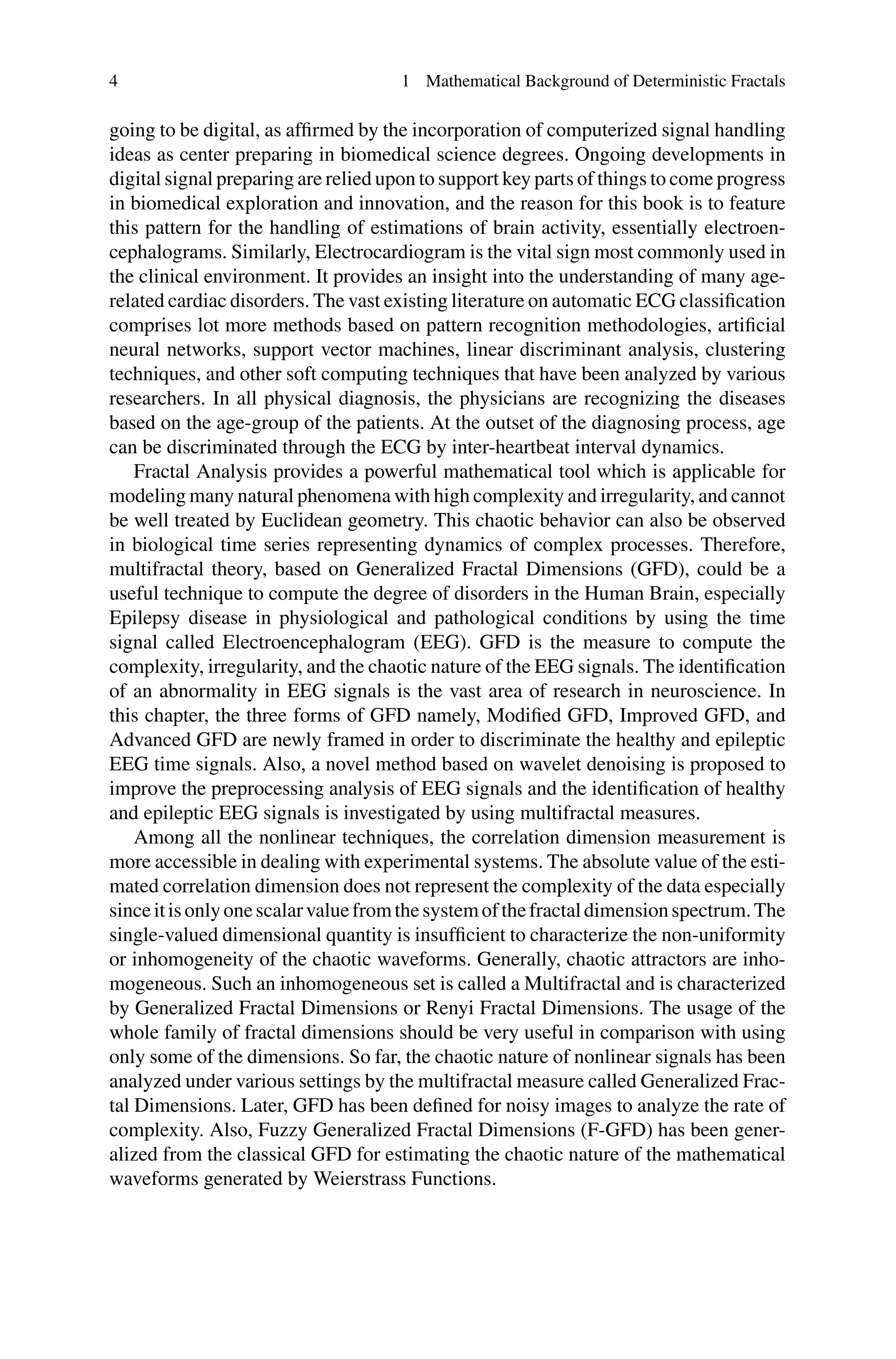
Fractal Analysis provides a powerful mathematical tool which is applicable for
modeling many natural phenomena with high complexity and irregularity, and cannot
be well treated by Euclidean geometry. This chaotic behavior can also be observed
in biological time series representing dynamics of complex processes. Therefore,
multifractal theory, based on Generalized Fractal Dimensions (GFD), could be a
useful technique to compute the degree of disorders in the Human Brain, especially
Epilepsy disease in physiological and pathological conditions by using the time
signal called Electroencephalogram (EEG). GFD is the measure to compute the
complexity, irregularity, and the chaotic nature of the EEG signals. The identification
of an abnormality in EEG signals is the vast area of research in neuroscience. In
this chapter, the three forms of GFD namely, Modified GFD, Improved GFD, and
Advanced GFD are newly framed in order to discriminate the healthy and epileptic
EEG time signals. Also, a novel method based on wavelet denoising is proposed to
improve the preprocessing analysis of EEG signals and the identification of healthy
and epileptic EEG signals is investigated by using multifractal measures.
Among all the nonlinear techniques, the correlation dimension measurement is
more accessible in dealing with experimental systems. The absolute value of the esti-
mated correlation dimension does not represent the complexity of the data especially
sinceitisonlyonescalarvaluefromthesystemofthefractaldimensionspectrum.The
single-valued dimensional quantity is insufficient to characterize the non-uniformity
or inhomogeneity of the chaotic waveforms. Generally, chaotic attractors are inho-
mogeneous. Such an inhomogeneous set is called a Multifractal and is characterized
by Generalized Fractal Dimensions or Renyi Fractal Dimensions. The usage of the
whole family of fractal dimensions should be very useful in comparison with using
only some of the dimensions. So far, the chaotic nature of nonlinear signals has been
analyzed under various settings by the multifractal measure called Generalized Frac-
tal Dimensions. Later, GFD has been defined for noisy images to analyze the rate of
complexity. Also, Fuzzy Generalized Fractal Dimensions (F-GFD) has been gener-
alized from the classical GFD for estimating the chaotic nature of the mathematical
waveforms generated by Weierstrass Functions.
19.
1.1 Introduction 5
Theaim of this chapter is to describe the fundamental concepts of deterministic
fractals in view of their use in fractal interpolation functions. This chapter will thus
present a modest introduction to the concepts of fixed point theorem, iterated func-
tion systems, and fractal dimensions. Since we are interested in fractal interpolation,
most theoretical results are given without proofs which are available in the references
mentioned where appropriate. This chapter first describes the deterministic fractal
through the several notions of iterated function systems which provide a global char-
acterization of a fractal. All the concepts presented here are more fully established
in [4]. The idea of dimension applies to sets in a metric space more broad than sig-
nals. Although the notion of dimension makes sense for more complex entities, for
example, measures or classes of functions, several interesting concepts of dimension
exist. Hence, the concept of fractal dimensions is concisely discussed at the end of
this chapter.
1.2 Iterated Function System
Hutchinson introduced the conventional explanation of deterministic fractals through
the theory of the iterated function system. Meanwhile, Barnsley formulated the the-
ory of the iterated function system called the Hutchinson–Barnsley theory in order to
define and construct the fractals as a non-empty compact invariant subset of a com-
plete metric space generated by the Banach fixed point theorem (for further reading,
[2, 3, 7–9]). This section concisely discusses the construction of deterministic frac-
tals (or metric fractals) in the complete metric space generated by the IFS of Banach
contractions.
Definition 1.1 A self-mapping f on the metric space (X, d) is called a contraction
mapping (simply contraction) if there exists a constant α ∈ [0, 1) such that
d( f (x), f (y)) ≤ αd(x, y) for all x, y ∈ X. (1.1)
The constant α is called the contraction factor or contraction ratio.
Definition 1.2 (fixed point) A point x in a metric space (X, d) is said to be a fixed
point of the mapping f : X → X, if x satisfies the equation f (x) − x = 0.
The fixed point of the given function f is invariant under the mapping f , hence it
is also known as an invariant point. Fixed points of the function f defined on R
are the points of intersection of the curve y = f (x) and the line y = x, as shown
in Fig.1.1. An identity function that is defined on R has all the points in R as fixed
points, whereas in the same domain f (x) = x2
has two fixed points namely, 1, 0.
Consider that the function f (x) = x2
− 1 on R does not have a fixed point in R.
These examples show that all the functions not necessarily have a unique fixed point
on their domain. The notable result which gives the uniqueness of a fixed point in a
complete metric space was explored by Stefan Banach in 1922.
20.
6 1 MathematicalBackground of Deterministic Fractals
-0.2 0 0.2 0.4 0.6 0.8 1 1.2
-0.2
0
0.2
0.4
0.6
0.8
1
1.2
1.4
1.6
-1 -0.5 0 0.5 1
-1.5
-1
-0.5
0
0.5
1
1.5
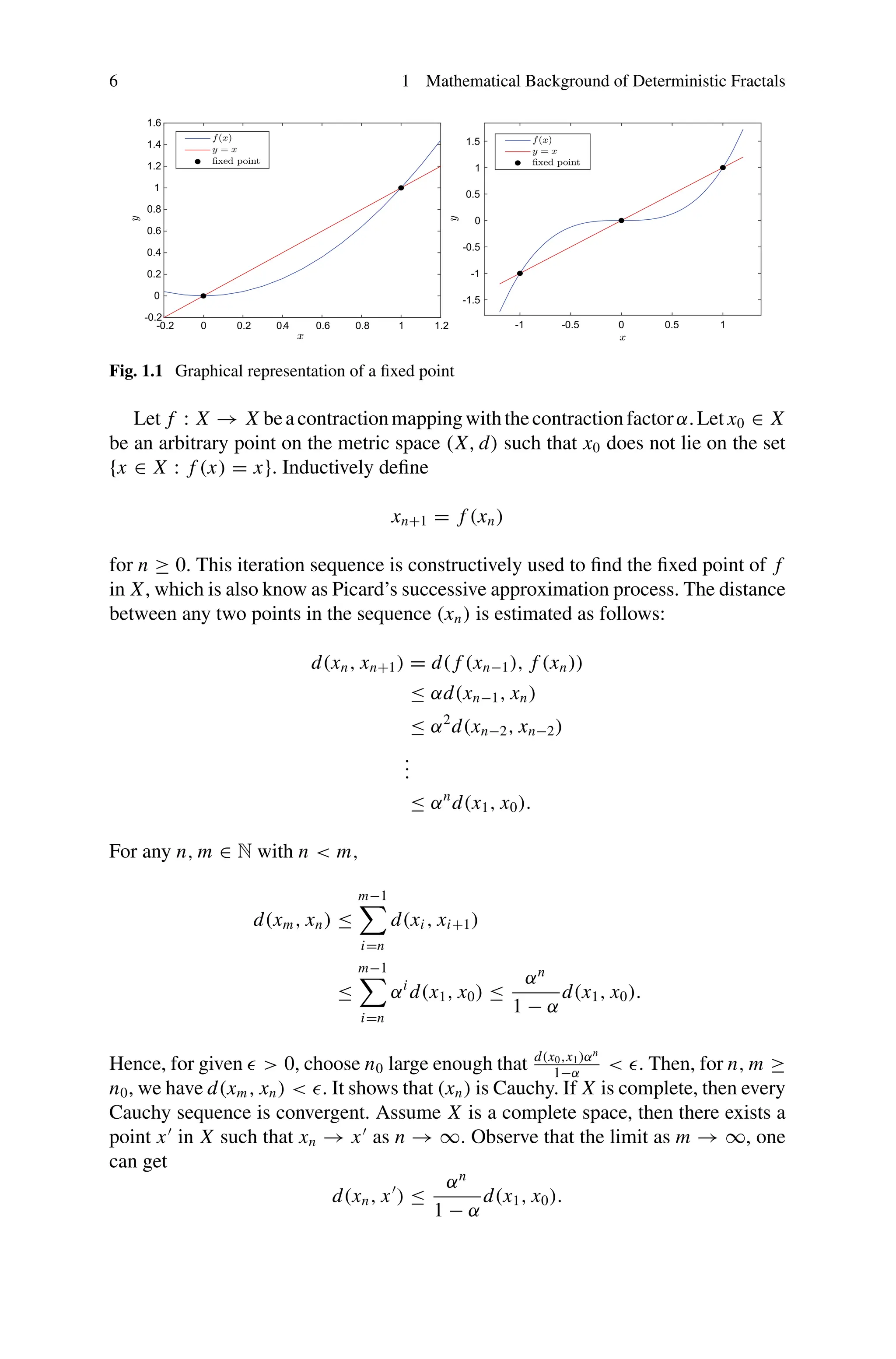
Fig. 1.1 Graphical representation of a fixed point
Let f : X → X beacontractionmappingwiththecontractionfactorα.Let x0 ∈ X
be an arbitrary point on the metric space (X, d) such that x0 does not lie on the set
{x ∈ X : f (x) = x}. Inductively define
xn+1 = f (xn)
for n ≥ 0. This iteration sequence is constructively used to find the fixed point of f
in X, which is also know as Picard’s successive approximation process. The distance
between any two points in the sequence (xn) is estimated as follows:
d(xn, xn+1) = d( f (xn−1), f (xn))
≤ αd(xn−1, xn)
≤ α2
d(xn−2, xn−2)
.
.
.
≤ αn
d(x1, x0).
For any n, m ∈ N with n < m,
d(xm, xn) ≤
m−1
i=n
d(xi , xi+1)
≤
m−1
i=n
αi
d(x1, x0) ≤
αn
1 − α
d(x1, x0).
Hence, for given 0, choose n0 large enough that d(x0,x1)αn
1−α
. Then, for n, m ≥
n0, we have d(xm, xn) . It shows that (xn) is Cauchy. If X is complete, then every
Cauchy sequence is convergent. Assume X is a complete space, then there exists a
point x
in X such that xn → x
as n → ∞. Observe that the limit as m → ∞, one
can get
d(xn, x
) ≤
αn
1 − α
d(x1, x0).
21.
1.2 Iterated FunctionSystem 7
This inequality gives explicit error estimation in xn when regarded as an estimate
of the fixed point x. Initially, we take the contraction mapping f and hence f
is uniformly continuous. Therefore, xn → x
implies f (xn) → f (x
). It follows
f (x
) = x
. Assume x
, y
are two points in X such that f (x
) = x
and f (y
) = y
.
Since f is a contraction mapping,
d(x
, y
) = d( f (x
), f (y
)) ≤ αd(x
, y
) d(x
, y
),
which implies d(x
, y
) = 0. Hence x
= y
.
The above argument summaries the following theorem namely, the Banach con-
traction principle.
Theorem 1.1 Let (X, d) be a complete metric space and f be a contraction mapping
on X. Then f has a unique fixed point x∗
.
The Banach contraction principle presented in Theorem 1.1 is applied in many
fields. In particular, this section describes an application of the Banach contraction
principle to the construction of fractals, widely known as the deterministic fractal, in
a complete metric space through iterated function systems. The study of fractals and
their properties in a complete metric space associated with the Banach contraction
principle is a constructive method to understand fractal geometry which is named as
the Hutchinson–Barnsley theory. For a large number of examples and details, refer
to the books ([2, 8, 9]).
Definition 1.3 For n ∈ N, let Nn denote the subset {1, 2, . . . , n} of N. Consider a
finite family of contraction mappings f1, f2, . . . , fn on X with contraction ratios
αk ∈ [0, 1), k ∈ Nn, simply written as ( fk)k∈Nn
. Then the system {X; fk : k ∈ Nn} is
called an Iterated Function System (IFS) or finite iterated function system.
Let (X, d) be a complete metric space and H(X) be the class of all non-empty
compact subsets of X. Usually, H(X) is known as a hyperspace of X which includes
all non-empty compact subsets of X. Define the distance between a point x in X and
a compact subset A in H(X) as follows:
d(x, A) = inf{d(x, a) : a ∈ A}. (1.2)
Now define the distance between two sets A, B ∈ H(X) as
d(A, B) = sup{d(a, B) : a ∈ A}. (1.3)
The Hausdorff distance between A and B in H(X) is defined as
Hd(A, B) = max{d(A, B), d(B, A)}. (1.4)
The hyperspace H(X) is complete with respect to the Hausdorff metric Hd.
Definition 1.4 Define the self-mapping F : H(X) −→ H(X) by
22.
8 1 MathematicalBackground of Deterministic Fractals
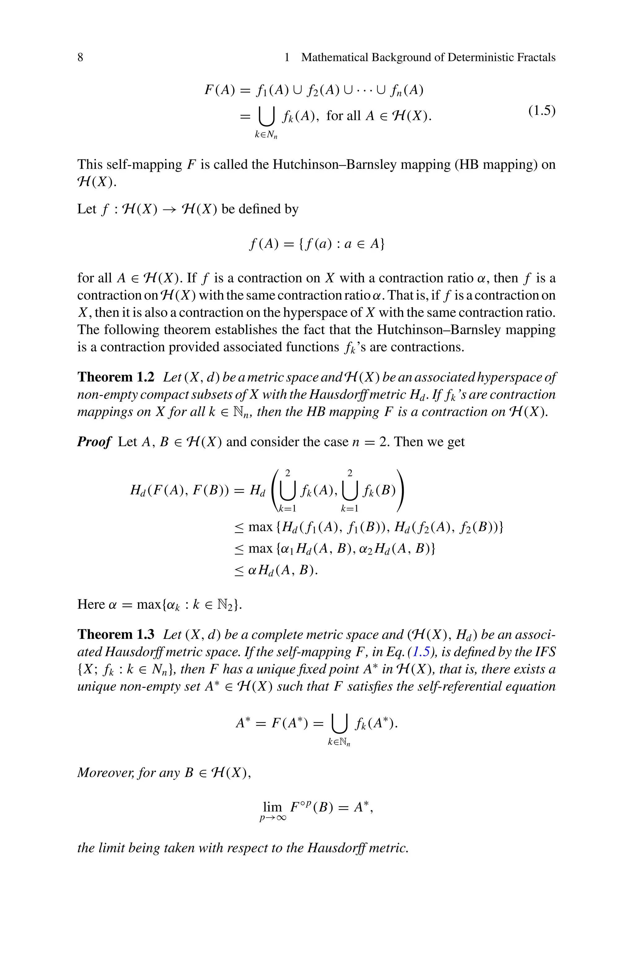
F(A) = f1(A) ∪ f2(A) ∪ · · · ∪ fn(A)
=
k∈Nn
fk(A), for all A ∈ H(X). (1.5)
This self-mapping F is called the Hutchinson–Barnsley mapping (HB mapping) on
H(X).
Let f : H(X) → H(X) be defined by
f (A) = { f (a) : a ∈ A}
for all A ∈ H(X). If f is a contraction on X with a contraction ratio α, then f is a
contractiononH(X)withthesamecontractionratioα.Thatis,if f isacontractionon
X, then it is also a contraction on the hyperspace of X with the same contraction ratio.
The following theorem establishes the fact that the Hutchinson–Barnsley mapping
is a contraction provided associated functions fk’s are contractions.
Theorem 1.2 Let(X, d)beametricspaceandH(X)beanassociatedhyperspaceof
non-empty compact subsets of X with the Hausdorff metric Hd . If fk’s are contraction
mappings on X for all k ∈ Nn, then the HB mapping F is a contraction on H(X).
Proof Let A, B ∈ H(X) and consider the case n = 2. Then we get
Hd(F(A), F(B)) = Hd
2
k=1
fk(A),
2
k=1
fk(B)
≤ max {Hd( f1(A), f1(B)), Hd( f2(A), f2(B))}
≤ max {α1 Hd(A, B), α2 Hd(A, B)}
≤ αHd(A, B).
Here α = max{αk : k ∈ N2}.
Theorem 1.3 Let (X, d) be a complete metric space and (H(X), Hd) be an associ-
ated Hausdorff metric space. If the self-mapping F, in Eq.(1.5), is defined by the IFS
{X; fk : k ∈ Nn}, then F has a unique fixed point A∗
in H(X), that is, there exists a
unique non-empty set A∗
∈ H(X) such that F satisfies the self-referential equation
A∗
= F(A∗
) =
k∈Nn
fk(A∗
).
Moreover, for any B ∈ H(X),
lim
p→∞
F◦p
(B) = A∗
,
the limit being taken with respect to the Hausdorff metric.
23.
1.2 Iterated FunctionSystem 9
-1
-0.8
-0.6
-0.4
-0.2
0
0.2
0.4
0.6
0.8
1
-1 -0.8 -0.6 -0.4 -0.2 0 0.2 0.4 0.6 0.8 1 -1 -0.5 0 0.5 1 1.5 2
-1.4
-1.2
-1
-0.8
-0.6
-0.4
-0.2
0
Fig. 1.2 Iteration of function
Proof The completeness of the space (X, d) gives (H(X), Hd) which is a complete
metric space. Theorem 1.2 shows that F is a contraction mapping on H(X). Hence,
by the Banach fixed point theorem 1.1, the contraction mapping F on the complete
metric space (H(X), Hd) has a unique fixed point. This completes the proof.
In Theorem 1.3, F◦p
denotes the pth composition of the HB mapping F, that is,
F◦p
= F ◦ F ◦ · · · ◦ F
p times
. The iteration of function is described in Fig.1.2.
Definition 1.5 A non-empty compact set A∗
obtained from Theorem 1.3 is called
an invariant set or self-referential set or attractor or deterministic fractal of the IFS
{X; fk : k ∈ Nn} .
Due to the sophisticated usage of fractals in nonlinear approximation, there are
sequel efforts to extend the Hutchinson–Barnsley classical framework for fractals to
more general spaces and countable IFS or infinite IFS [28–37]. Consequent sections
review some basic definitions and results on the theory of the generalized iterated
function system and its attractors.
1.3 Countable Iterated Function System
The Hutchinson–Barnsley theory of finite iterated function systems has been stud-
ied in the last decades with some extensions of the spaces and the contractions of
various types. In this section, an extension of the Hutchinson–Barnsley theory of
finite iterated function systems to a countable iterated function system is presented.
N.A. Secelean has generalized the HB theory by constructing the deterministic frac-
tals through a countable iterated function system [28]. After a brief review of the
fundamental properties of a countable iterated function system (CIFS), this section
describes the features and approximation of attractor of CIFS with the attractors of
IFS.
24.
10 1 MathematicalBackground of Deterministic Fractals
Consider the sequence of Banach contractions ( fn)n≥1 on a compact metric space
X with contraction factors rn ∈ [0, 1), n ≥ 1. Then the system {X; fn : n ≥ 1} is
called a Countable Iterated Function System (CIFS).
Define a self-map F : H(X) −→ H(X) by
F(B) =
∞
n=1
fn(B), for all B ∈ H(X). (1.6)
Then the self-map F is a Banach contraction with a contraction factor r ≤ suprn,
n ≥ 1.
Theorem 1.4 The self-map F defined in Eq.(1.6) has a unique fixed point A ∗
,
that is, there exists a unique non-empty set A ∗
∈ K (X) such that F satisfies the
self-referential equation
A ∗
= F(A ∗
) =
∞
n=1
fn(A ∗).
Furthermore, for any B ∈ H(X), limn→∞ F◦n
(B) = A ∗
, the limit being taken
with respect to the Hausdorff metric.
A non-empty compact invariant set A ∗
obtained from Theorem 1.4 is called an
attractor of the CIFS {X; fn : n ≥ 1}. The attractor A ∗
is known as a deterministic
fractal generated by the CIFS of contractions.
According to Theorem 1.3, the attractor A∗
is dependent on the corresponding
IFS. Suppose A∗
N is an attractor of the IFS {X; fn : n = 1, 2, . . . , N} and FN is
the associated HB operator, for N ≥ 1. Then, the following Theorem 1.5 reveals the
relation between the attractors of IFS and the attractor of CIFS of Banach contractions
on a compact metric space X.
Theorem 1.5 If B ∈ H(X), then
F(B) = lim
N→∞
FN (B) = lim
N→∞
N
n=1
fn(B).
In particular, if A is the attractor of CIFS {X; fn : n ≥ 1}, then
A = F(A ) = lim
N→∞
A∗
N = lim
N→∞
lim
n→∞
F◦n
N (B),
also, A = limN→∞ limn→∞ F◦n
N (B).
The above theorem shows that the attractor of CIFS {X; fn : n ≥ 1} is approxi-
mated by the attractors of IFS {X; fn : n = 1, 2, . . . , N} , N ≥ 1, with respect to the
Hausdorff metric.
25.
1.3 Countable IteratedFunction System 11
Example 1.1 Consider the space X = [0, 1] with the Euclidean metric. Let q ∈
(0, 1
2
], define fn : [0, 1] −→ [0, 1] by fn(x) = qn
x + αn, for all n ∈ N, where
α1 = 0 and αn = qn−1
+ 1−2q
2−3q
n−1
+ αn−1, n ≥ 2. Then the attractor of the CIFS
{X; fn : n ≥ 1} gives the infinite type Cantor set.
If q = 1/3 and αn = 1 − 1
3
n−1
, n ≥ 1, then the sequence of Banach contrac-
tions becomes fn = x
3n + 1 − 1
3n−1
, n ≥ 1.
Example 1.2 Let X = [0, 1] × [0, 1] ⊂ R2
, for every n = 4p + k, consider the fol-
lowing contractions:
fn(x, y) =
⎧
⎪
⎪
⎪
⎪
⎨
⎪
⎪
⎪
⎪
⎩
1
2p+1
1
3
x + 2p+1
− 2, 1
3
y , if k = 1,
1
2p+1
1
6
x −
√
3
6
y + 2p+1
− 5,
√
3
6
x + 1
6
y , if k = 2,
1
2p+1
1
6
x +
√
3
6
y + 2p+1
− 3
2
, −
√
3
6
x + 1
6
y +
√
3
6
, if k = 3,
1
2p+1
1
3
x + 2p+1
− 4
3
, 1
3
y , if k = 4.
Then the attractor of the CIFS {X; fn : n ≥ 1} gives the infinite type von Koch
curve.
1.4 Local Countable Iterated Function System
This section concisely provides the essential material of a local iterated function
system (LIFS) and describes the approximation process of the attractor of a local
countable iterated function system with the attractors of the iterated function system.
1.4.1 Local Iterated Function System
If {Xi : i ∈ Nn} is n number of non-empty subsets of X and for each Xi , there exists
a continuous mapping fi on Xi to X. Then the system {X; (Xi , fi ) : i ∈ N} is called
a local iterated function system (local IFS) [6] whereas, an iterated function system
(IFS) is a complete metric space X together with a finite set of contraction mappings,
denoted by {X; fk : k ∈ Nn}, with contraction factors ck, k ∈ Nn . If Xi = X, then
local IFS becomes (global) IFS. The operator Floc,n on H(X) is defined by
Floc,n(B) =
i∈Nn
fi (B ∩ Xi ).
Here fi (S ∩ Xi ) = { fi (x) : x ∈ S ∩ Xi }.
26.
12 1 MathematicalBackground of Deterministic Fractals
Theorem 1.6 Let X be a complete metric space with the Hausdorff metric. Let (En)n
be a sequence of compact subsets of X such that En ⊂ En+1 and E =
∞
n=1 En. Then
Ē = limn→∞ En.
1.4.2 Existence and Analytical Properties of LCIFS
Suppose {Xi : i ∈ N} is a sequence of non-empty subsets of X. Further assume
that for each Xi , there exists a continuous mapping fi : Xi −→ X, i ∈ N. Then
{X; (Xi , fi ) : i ∈ N} is called a local countable iterated function system (local CIFS).
If Xi = X, then local CIFS becomes global CIFS. A local CIFS is called contractive
or hyperbolic if each fi is a contraction on their respective domains.
Let P(X) be the power set of X, i.e., P(X) = {S : S ⊂ X}. Define Wloc :
P(X) −→ P(X) by
Wloc(B) =
i∈N
fi (B ∩ Xi ).
Here fi (S ∩ Xi ) = { fi (x) : x ∈ S ∩ Xi }.
Every local CIFS has at least one local attractor (fixed point of Wloc ) namely,
A = ∅, empty set. The largest local attractor, union of all distinct local attractors, is
called the local attractor of local CIFS, {X; (Xi , fi ) : i ∈ Nn}. If X is compact and
Xi , i ∈ N, is closed, the compact in X and where local CIFS {X; (Xi , fi ) : i ∈ Nn}
is contractive, the local attractor may be computed as follow.
Let K0 = X and set
Kn = Wloc(Kn−1) =
i∈N
fi (Ki−1 ∩ Xi ), n ∈ N.
Then {Kn : n ∈ N} is a decreasing nested sequence of compact sets. If each Kn is
non-empty, then by the cantor intersection theorem,
K =
n∈N
Kn = ∅
K = lim
n→∞
Kn,
limit taken with respect to the Hausdorff metric Hd on K (X).
27.
1.4 Local CountableIterated Function System 13
K = lim
n→∞
Kn = lim
n→∞
i∈N
fi (Kn−1 ∩ Xi )
=
i∈N
fi (K ∩ Xi )
= Wloc(K).
Thus, K = Aloc.Aconditionguaranteeingthateach Kn isnon-emptyisthat fi (Xi ) ⊂
Xi , i ∈ N.
Theorem 1.7 Let X be a compact metric space and let Xi , i ∈ N, be a closed subset
of X. If A is an attractor of CIFS and A∗
is a local attractor of local CIFS, then A∗
is a subset of A.
Proof Consider the sequence {Kn : n ∈ N} such that K0 = X and Kn = Wloc
(Kn−1) =
i∈N fi (Ki−1 ∩ Xi ), n ∈ N. The unique attractor A is obtained as the
limit of the sequence {Kn : n ∈ N}. Let {X; fi : i ∈ Nn} be the contractive CIFS asso-
ciated with the set-valued map W on H(X) defined by W(B) =
i∈N fi (B). Then,
the unique attractor A of the CIFS is obtained as the limit of the sequence {An : n ∈
N} such that A0 = X and An = W(An−1), n ∈ N. Assume Kn−1 ⊆ An−1, n ∈ N,
we have
A∗
= lim
n→∞
Kn = lim
n→∞
i∈N
fi (Kn−1 ∩ Xi )
⊆ lim
n→∞
i∈N
fi (Kn−1)
⊆ lim
n→∞
i∈N
fi (An−1) = lim
n→∞
An = A.
Theorem1.7 reveals the relation between the attractor of a countable iterated func-
tion system and a local countable iterated function system.
Theorem 1.8 Let X be a compact metric space. Let {X; (Xi , fi ) : i ∈ N} be a local
CIFS and {X; (Xi , fi ) : i ∈ Nn} be a local IFS. Suppose limn→∞ En = E = ∅,
where each n, En ⊆ X. Then the local attractor A∗
of CIFS is approximated by
the local attractors A’s of local IFSs.
lim
n
lim
k
Fk
loc,n(En) = A∗
.
Proof Let Floc,n(B) =
i∈Nn
fi (B ∩ Xi ), for n ∈ N. Then it’s enough to prove that
lim
n→∞
Fk
loc,n(En) = Wk
loc(E), (1.7)
where the limit is taken with respect to the Hausdorff metric h. As {X; (Xi , fi ) :
i ∈ Nn} is a local IFS, for each Xi there exists a contraction mapping fi : Xi →
28.
14 1 MathematicalBackground of Deterministic Fractals
X with contraction factors ci , i ∈ Nn. Denote fi1...ik
= fi1
◦ · · · ◦ fik
, for each k ≥
1, i1, i2, . . . , ik are positive integers. Clearly, fi1...ik
is a contraction mapping with
contraction factor ci1
ci2
· · · cik
.
h(Fk
loc,n(En), Wk
loc(E)) ≤ h(Fk
loc,n(En), Fk
loc,n(E)) + h(Fk
loc,n(E), Wk
loc(E)).
(1.8)
The first term of the left-hand side of Eq.(1.8) can be expressed as
h(Fk
loc,n(En), Fk
loc,n(E)) = h
⎛
⎝
i1,...,ik ∈Nn
fi1...ik
(En ∩ Xn),
i1,...,ik ∈Nn
fi1...ik
(E ∩ Xn)
⎞
⎠
(1.9)
≤ sup
i1,...,ik ∈Nn
h( fi1...ik
(En ∩ Xn), fi1...ik
(E ∩ Xn))
≤ ci1
· · · cik
h(En ∩ Xn, E ∩ Xn)
≤ h(En, E).
Since limn→∞ En = E, h(En, E) → 0 as n → ∞. Now, let us consider the second
term in Eq.(1.8).
Wk
loc(B) =
i1,...,ik ∈N
fi1...ik
(B). (1.10)
Continuity of fi ’s and the basic topological result give the following:
Wk+1
loc (E) = Wloc
⎛
⎝
i1,...,ik ∈N
fi1...ik
(E)
⎞
⎠
=
∞
i=1
fi
⎛
⎝
i1,...,ik ∈N
fi1...ik
(E ∩ Xi )
⎞
⎠
⊂
∞
i=1
fi
⎛
⎝
i1,...,ik ∈N
fi1...ik
(E ∩ Xi )
⎞
⎠
=
∞
i=1
fi
⎛
⎝
i1,...,ik ∈N
fi1...ik
(E ∩ Xi )
⎞
⎠ = Wk+1
loc (E).
The sequence of sets
i1,...,ik ∈Nn
fi1...ik
(E ∩ Xn) n∈N
is increasing and by Theorem
(1.6)
29.
1.4 Local CountableIterated Function System 15
lim
n→∞
Fk
loc,n(E) = lim
n→∞
i1,...,ik ∈Nn
fi1...ik
(E ∩ Xn) (1.11)
=
∞
n=1
i1,...,ik ∈Nn
fi1...ik
(E ∩ Xn)
=
i1,...,ik ∈N
fi1...ik
(E) = Wk
loc(E).
Applying Eqs.(1.9), (1.11) in (1.8) gives h(Fk
loc,n(En), Wk
loc(E)) = 0 as n, k → 0.
Thus we conclude,
lim
n→∞
lim
k→∞
Fk
loc,n(En) = lim
k→∞
Wk
loc(E) = A∗
.
Theorem1.8 establishes the approximation process of the attractor of the local
iterated function system in terms of attractors of a local countable iterated function
system.
1.5 Fractal Dimension
Measuring the size of a set or an object helps to understand its fundamental nature.
In mathematics, objects are constituted by set of points, lines, square or cubes. How
do we measure the size of a set? For instance, consider a straight line with length L.
The approximate length L() is estimated by the product of the number N() of line
segment of length (yardstick) required to cover the straight line, i.e.,
× N() = L(). (1.12)
As yardstick tends to zero, it makes L() approach the length L of the straight line,
i.e.,
lim
→0
× N() = L. (1.13)
There exists a positive integer n such that ≥ /n and if the length L is measured
by a smaller size of the yardstick /n, then
/n × N(/n) = L. (1.14)
It gives that
N(/n) = nN(). (1.15)
Extending this idea to a higher dimensional space gives
30.
16 1 MathematicalBackground of Deterministic Fractals
N(/n) = nd
N(), (1.16)
where d = 1, 2, 3, . . .. It implies that if the size of the yardstick is decreased by a
factor of n, then the numerical value of the number N is increased by a factor of
nd
. It can be rigorously proved that the solution of Eq.(1.16) is given by the inverse
power law
N() ∼
1
d
, (1.17)
where d = 1, 2, 3. The integer solution of Eq.(1.17) is known as the Euclidean
dimension of the given object. If the object is a fractal, then
lim
→0
× N() = ∞.
Since, if the size of the yardstick is decreased, then one can get a finer and finer fractal
structure, hence N() is large. However, in this case, Eq.(1.17) has a non-integer
solution which is known as the Hausdorff dimension. The Hausdorff dimension is
defined as follows. If U is any non-empty subset of n-dimensional Euclidean space
Rn
, the diameter of U is defined as
|U| = sup{|x − y| : x, y ∈ U},
i.e., the greatest distance apart from any pair of points in U. If {Ui } is a countable
(or finite) collection of sets of diameter at most δ that cover F, i.e.,
K ⊂
∞
i=1
Ui
with 0 |Ui | ≤ δ for each i, we say that {Ui } is a δ-cover of K. Suppose that K is
a subset of Rn
and s is a non-negative number. For any δ 0, we define
Hs
δ (K) = inf
∞
i=1
|Ui |s
: {Ui } is a δ-cover of K
.
As δ decreases, the class of permissible covers of K is reduced. Therefore, the
infimum Hs
δ (K) increases, and so approaches a limit as δ → 0. Thus,
Hs
(K) = lim
δ→0
Hs
δ (K).
This limit exists for any subset K of Rn
, though the limiting value can be 0 or ∞.
We call Hs
(K) as the s-dimensional Hausdorff measure of K. Then, the Hausdorff
Dimension or Hausdorff–Besicovitch Dimension of K is defined as
dimH (K) = inf
s : Hs
(K) = 0
= sup
s : Hs
(K) = ∞
,
31.
1.5 Fractal Dimension17
so that
Hs
(K) =
∞, if s dimH (K),
0, if s dimH (K).
If s = dimH (K), then Hs
(K) may be zero or infinite, or may be 0 Hs
(K) ∞.
The Hausdorff dimension has the advantage of being defined for any set, and is
mathematically convenient, as it is based on measures, which are relatively easy to
manipulate. The main disadvantage is that the explicit computation of the Hausdorff
dimension of a given set K is rather difficult since it involves taking the infimum
over covers consisting of balls of radius less than or equal to a given 0. A slight
simplification is obtained by considering only covers by the balls of radius equal to
. This gives rise to the concepts of the box dimension [8].
Let K ∈ H(X) and N() denote the smallest number of closed balls of radius
0 required to cover K. If
dimB = lim
→0
log N()
log(1/)
(1.18)
exists, then dimB is called the box dimension or fractal dimension of K.
Suppose that K is a subset in Rn
. The topological dimension of K, denoted as
dimT M, is inductively defined as follows:
1. dimT ∅ = −1,
2. The topological dimension of K at a point p ∈ K is less than or equal to n,
written as dim
p
T K ≤ n, if there exist arbitrarily small neighborhood of p whose
boundaries have a topological dimension at most n − 1,
3. K has a topological dimension at most n if it has a topological dimension at most
n at each of its points p:
dimT K ≤ n ⇐⇒ dim
p
T K ≤ n for all p ∈ K.
In addition, dim
p
T K = ∞, if condition (2) does not hold for any n ∈ N, and
dimT K = ∞ if condition (3) does not hold for any n ∈ N.
1.6 Generalized Fractal Dimensions
Fractal dimension is insufficient to characterize the object of interest having complex
and inhomogeneous scaling properties, since different irregular structures may have
the same fractal dimension [70, 71]. Thus, generalized fractal dimensions provide
more information about the space filling properties than the fractal dimension alone
(see, for instance, [1]). This section describes the generalized fractal dimensions
through Renyi entropy as follows.
32.
18 1 MathematicalBackground of Deterministic Fractals
Alfred Renyi introduced the measure to quantify the uncertainty or randomness
of a given system. It plays a vital role in the information theory [75].
Given probabilities pi ,
N
i=1 pi = 1, the Renyi entropy of order q is given by
REq =
1
1 − q
log
N
i=1
p
q
i ,
where q ≥ 0 and q = 1. At q = 1, the value of REq is potentially undefined as it
generates the indeterminate form, otherwise REq values are decreasing as a function
of q.
If q → 1, then REq → RE1 which is defined by
RE1 = −ln
N
i=1
pi log pi .
RE1 is called Shannon entropy. Renyi Fractal Dimensions or Generalized Fractal
Dimensions (GFD) of order q ∈ (−∞, ∞) are defined, in terms of generalized Renyi
Entropy, as
Dq = lim
r→0
1
q − 1
log2
N
i=1 p
q
i
log2 r
(1.19)
where pi is the probability distribution. For all q, we have Dq 0 and Dq is a
monotonically decreasing function of q such that D0 ≥ D1 ≥ D2. Also, observe that
Dq = D0 = 0, for all q for a constant signal because all probabilities except one
equal to zero, whereas the exceptional probability value is one.
1.6.1 Some Special Cases
• If q = 0, then
D0 =
log2 N
log2 r
, (1.20)
which is known as the Fractal Dimension.
• As q −→ 1, Dq converges to D1, which is given by
D1 = lim
r→0
N
i=1 pi log2 pi
log2 r
, (1.21)
where D1 is the Information Dimension
• If q = 2, then Dq is called the Correlation Dimension.
Welcome to ourwebsite – the ideal destination for book lovers and
knowledge seekers. With a mission to inspire endlessly, we offer a
vast collection of books, ranging from classic literary works to
specialized publications, self-development books, and children's
literature. Each book is a new journey of discovery, expanding
knowledge and enriching the soul of the reade
Our website is not just a platform for buying books, but a bridge
connecting readers to the timeless values of culture and wisdom. With
an elegant, user-friendly interface and an intelligent search system,
we are committed to providing a quick and convenient shopping
experience. Additionally, our special promotions and home delivery
services ensure that you save time and fully enjoy the joy of reading.
Let us accompany you on the journey of exploring knowledge and
personal growth!
textbookfull.com


![Chapter 1
Mathematical Background of
Deterministic Fractals
1.1 Introduction
The historical backdrop of describing natural objects by mathematics, with respect
to Euclidean geometry, is as old as the advent of science itself. In our intuitive
understanding, traditionally lines, squares, rectangles, circles, spheres, and so forth
have been the fundamental shapes of geometry. Mathematics is mostly concerned
with these fundamental shapes to model or approximate or often analyze the nat-
ural phenomena. Indeed, nature is not confined to such Euclidean entities thatare
typically characterized only by integer dimensions, but we restricted ourselves to
integer dimensions only. Actually, even now in the beginning phase of our teaching,
we discover that objects which have just length are one dimensional, objects with
length and width are two dimensional, and those that have length, width, and breadth
are three dimensional. Did we ever raise the question for what reason we are always
moving toward integer dimension? The response as far as we could possibly know
is Never. We never addressed such a question, if there exist objects with non-integer
dimensions. However, one person did and he was none other than Benoit B. Man-
delbrot. He included another word in the scientific jargon through his inventive work
which he termed as a fractal. He was bewildered with such thoughts for many years
and realized that nature is not restricted to Euclidean or integer-dimensional space.
Rather, a large portion of the natural objects which we see around us are complex in
shape, and traditional Euclidean geometry is not adequate to depict them. The notion
of fractal geometry has all the earmarks of being irreplaceable for portraying such
complex structure at least quantitatively. Mandelbrot has revolutionized Euclidean
geometry with the notion of a fractal that has generated extensive attention in almost
every branch of science. He presented his new concept through his amazing book
“The fractal geometry of nature ”in a striking manner and since then it stayed as the
standard reference book for both amateurs and scientists [1]. In a sense, the idea of a
fractal has brought numerous apparently disconnected subjects under one umbrella.
© The Author(s), under exclusive license to Springer Nature Switzerland AG 2021
S. Banerjee et al., Fractal Functions, Dimensions and Signal Analysis,
Understanding Complex Systems, https://doi.org/10.1007/978-3-030-62672-3_1
1](https://image.slidesharecdn.com/85835-250720042349-23fa1e14/75/Fractal-Functions-Dimensions-and-Signal-Analysis-Santo-Banerjee-15-2048.jpg)
![2 1 Mathematical Background of Deterministic Fractals
There has been a surge of research activities in applying the influential fractal
idea in pretty much every part of scientific disciplines to increase profound bits of
knowledge into numerous unresolved problems. However, there is no flawless and
complete definition of the fractal. The simplest way to define a fractal is as an object
which appears self-similar under varying degrees of magnification. A ‘Fractal’ is
generally a rough or fragmented geometric shape that can be split into parts, each of
which is (at least approximately) a reduced-size copy of the whole, a property called
self-similarity. The word Fractal is derived from the Latin word, fractus meaning
broken or fractured to describe objects that were too irregular to fit into a traditional
geometrical setting. In Mandelbrot’s original article, the Fractal is mathematically
defined as a set with the Hausdorff dimension strictly greater than its topological
dimension. Roughly speaking, a fractal set is a set that is more ‘irregular’ than the
sets considered in classical geometry. Fractal sets have the additional property of
being in some sense either strictly or statistically self-similar; this property has been
widely applied to model the numerous natural phenomena by Mandelbrot and oth-
ers. However, the notion of the strict self-similar property has been theoretically
framed by Hutchinson and popularized by Barnsley. The iterated function system is
a convenient and powerful way tool for generating fractals in a metric space with
specified self-similarity properties. Hutchinson introduced the conventional expla-
nation of deterministic fractals through the theory of Iterated Function System (IFS).
Meanwhile, Barnsley formulated the theory of IFS called the Hutchinson–Barnsley
(HB) theory in order to define and construct the fractals as a non-empty compact
invariant subset of a complete metric space which is generated by the Banach fixed
point theorem, known as IFS theory [2, 3]. In view of the applications of fractals to
comprehend the natural phenomena, every area of science has been concerned about
the fractal analysis. Hence, fractal analysis plays a central role in mathematics as a
tool for nonlinear applications and as a theory of interest.
Karl Weierstrass gave an example of a function with the non-intuitive property of
being everywhere continuous but nowhere differentiable, called Weierstrass Func-
tion, whose graph would today be considered as a fractal. The complexity and irreg-
ularity can be found in many physical and biological nonlinear systems naturally and
have been analyzed by the tools of fractal theory and computed by the non-integer or
fractional measure called Fractal Dimension. In approximation theory, the traditional
interpolation techniques generate a smooth or piecewise differentiable interpolation
function, despite the data points being irregular. Nevertheless, most of the natural
objects such as lightning, clouds, mountain ranges, and wall cracks have irregular
and complex structures in which Euclidean geometry cannot be applied successfully
to describe them. Hence, there is a need for a nonlinear tool in the approximation
theory to resolve these problems. M. F. Barnsley invented the Fractal Interpolation
Function (FIF) based on the theory of IFS, which precisely suited for the approxi-
mation of naturally occurring functions which possess some kind of self-similarity
under magnification [4]. Fractal interpolation functions are not necessarily differen-
tiable even though they are continuous everywhere. Hence, FIFs are sophisticated in
approximating the rough curve which precisely reconstructs the naturally occurring
functions when compared to the classical interpolants. Nevertheless, a smooth curve](https://image.slidesharecdn.com/85835-250720042349-23fa1e14/75/Fractal-Functions-Dimensions-and-Signal-Analysis-Santo-Banerjee-16-2048.jpg)
![1.1 Introduction 3
is needed to approximate some kind of functions which include the self-similarity
under magnification. Barnsley and Harrington explored the construction of p-times
frequently differentiable FIF when the derivative values reach up to pth order at the
initial endpoint of the interval [5].
During the past few years, numerous mathematical techniques were broadly cor-
related with fractal analysis. Considering the importance of fractional calculus for
discussing the variance ratio of fractal functions, the general relationship between
the fractional calculus and fractals has been investigated. Based on these studies,
there are continuous efforts connecting the fractional calculus, and the graphs of
the fractal function are available in the literature. Generally, the interpolation and
approximation of functions have been constructed by means of smooth functions,
often piecewise differentiable. However, the waves and signals from the real world
do not share this aspect. Hence, the main goal of the current book is to provide the
idea to approximate the rough (nowhere differentiable) functions through the fractal
interpolation function and its fractional calculus. Against this background, it is pro-
posed to generalize any interpolation function, smooth or rough, by means of a family
of fractal functions. It is also proposed to construct the various fractal interpolation
functions for a sequence of data and to investigate their shape-preserving properties.
Fractional calculus of such functions will be explored for approximating the rough
functions, additionally to correlate the fractional order and fractal dimension of the
fractal interpolation function.
The brain cells of humans start in between the 120th day and the 160th day of
pregnancy. It is accepted that from this beginning phase and throughout life, electri-
cal signals produced by the brain which speak to the cerebrum work as well as the
status of the entire body. In this direction, there are numerous advanced digital signal
processing methods applied on the biomedical signals, and thereby understand the
brain activity of a human. Signals from the human body play a vital role for the early
diagnosis of a variety of diseases. Such electrobiological signals can be in the form
of an electrocardiogram (ECG) taken from the heart, electromyogram (EMG) mea-
sured in muscles, electroencephalogram (EEG) from the brain, magnetoencephalo-
gram (MEG) given by the brain, electrogastrogram (EGG) from the stomach, and
electrooculogram (EOG) generated by eye nerves. As an application part, this book
discusses the signal analysis with respect to a multifractal perspective. Particularly,
fractal methods are applied on a medical signal, such as an Electroencephalogram
and Electrocardiogram, to help in the diagnosis. An EEG signal is a capacity of
currents that flow during synaptic excitations of the dendrites of many pyramidal
neurons in the cerebral cortex. The synaptic currents are formed within the dendrite
when neurons are activated. This current produces a magnetic field measurable by
electromyogram machines and a secondary electrical field over the scalp measurable
by EEG systems. There is ever-expanding worldwide interest for more moderate
and powerful clinical and medicinal services. New strategies and apparatus should
be created along these lines to help in the diagnosis, monitoring, and treatment of
abnormalities and diseases of the human body. Biomedical signs (biosignals) in their
complex structures are rich data sources, which when properly prepared can possibly
encourage such developments. In the present revolution, such preparing is probably](https://image.slidesharecdn.com/85835-250720042349-23fa1e14/75/Fractal-Functions-Dimensions-and-Signal-Analysis-Santo-Banerjee-17-2048.jpg)
![1.1 Introduction 5
The aim of this chapter is to describe the fundamental concepts of deterministic
fractals in view of their use in fractal interpolation functions. This chapter will thus
present a modest introduction to the concepts of fixed point theorem, iterated func-
tion systems, and fractal dimensions. Since we are interested in fractal interpolation,
most theoretical results are given without proofs which are available in the references
mentioned where appropriate. This chapter first describes the deterministic fractal
through the several notions of iterated function systems which provide a global char-
acterization of a fractal. All the concepts presented here are more fully established
in [4]. The idea of dimension applies to sets in a metric space more broad than sig-
nals. Although the notion of dimension makes sense for more complex entities, for
example, measures or classes of functions, several interesting concepts of dimension
exist. Hence, the concept of fractal dimensions is concisely discussed at the end of
this chapter.
1.2 Iterated Function System
Hutchinson introduced the conventional explanation of deterministic fractals through
the theory of the iterated function system. Meanwhile, Barnsley formulated the the-
ory of the iterated function system called the Hutchinson–Barnsley theory in order to
define and construct the fractals as a non-empty compact invariant subset of a com-
plete metric space generated by the Banach fixed point theorem (for further reading,
[2, 3, 7–9]). This section concisely discusses the construction of deterministic frac-
tals (or metric fractals) in the complete metric space generated by the IFS of Banach
contractions.
Definition 1.1 A self-mapping f on the metric space (X, d) is called a contraction
mapping (simply contraction) if there exists a constant α ∈ [0, 1) such that
d( f (x), f (y)) ≤ αd(x, y) for all x, y ∈ X. (1.1)
The constant α is called the contraction factor or contraction ratio.
Definition 1.2 (fixed point) A point x in a metric space (X, d) is said to be a fixed
point of the mapping f : X → X, if x satisfies the equation f (x) − x = 0.
The fixed point of the given function f is invariant under the mapping f , hence it
is also known as an invariant point. Fixed points of the function f defined on R
are the points of intersection of the curve y = f (x) and the line y = x, as shown
in Fig.1.1. An identity function that is defined on R has all the points in R as fixed
points, whereas in the same domain f (x) = x2
has two fixed points namely, 1, 0.
Consider that the function f (x) = x2
− 1 on R does not have a fixed point in R.
These examples show that all the functions not necessarily have a unique fixed point
on their domain. The notable result which gives the uniqueness of a fixed point in a
complete metric space was explored by Stefan Banach in 1922.](https://image.slidesharecdn.com/85835-250720042349-23fa1e14/75/Fractal-Functions-Dimensions-and-Signal-Analysis-Santo-Banerjee-19-2048.jpg)
![1.2 Iterated Function System 7
This inequality gives explicit error estimation in xn when regarded as an estimate
of the fixed point x. Initially, we take the contraction mapping f and hence f
is uniformly continuous. Therefore, xn → x
implies f (xn) → f (x
). It follows
f (x
) = x
. Assume x
, y
are two points in X such that f (x
) = x
and f (y
) = y
.
Since f is a contraction mapping,
d(x
, y
) = d( f (x
), f (y
)) ≤ αd(x
, y
) d(x
, y
),
which implies d(x
, y
) = 0. Hence x
= y
.
The above argument summaries the following theorem namely, the Banach con-
traction principle.
Theorem 1.1 Let (X, d) be a complete metric space and f be a contraction mapping
on X. Then f has a unique fixed point x∗
.
The Banach contraction principle presented in Theorem 1.1 is applied in many
fields. In particular, this section describes an application of the Banach contraction
principle to the construction of fractals, widely known as the deterministic fractal, in
a complete metric space through iterated function systems. The study of fractals and
their properties in a complete metric space associated with the Banach contraction
principle is a constructive method to understand fractal geometry which is named as
the Hutchinson–Barnsley theory. For a large number of examples and details, refer
to the books ([2, 8, 9]).
Definition 1.3 For n ∈ N, let Nn denote the subset {1, 2, . . . , n} of N. Consider a
finite family of contraction mappings f1, f2, . . . , fn on X with contraction ratios
αk ∈ [0, 1), k ∈ Nn, simply written as ( fk)k∈Nn
. Then the system {X; fk : k ∈ Nn} is
called an Iterated Function System (IFS) or finite iterated function system.
Let (X, d) be a complete metric space and H(X) be the class of all non-empty
compact subsets of X. Usually, H(X) is known as a hyperspace of X which includes
all non-empty compact subsets of X. Define the distance between a point x in X and
a compact subset A in H(X) as follows:
d(x, A) = inf{d(x, a) : a ∈ A}. (1.2)
Now define the distance between two sets A, B ∈ H(X) as
d(A, B) = sup{d(a, B) : a ∈ A}. (1.3)
The Hausdorff distance between A and B in H(X) is defined as
Hd(A, B) = max{d(A, B), d(B, A)}. (1.4)
The hyperspace H(X) is complete with respect to the Hausdorff metric Hd.
Definition 1.4 Define the self-mapping F : H(X) −→ H(X) by](https://image.slidesharecdn.com/85835-250720042349-23fa1e14/75/Fractal-Functions-Dimensions-and-Signal-Analysis-Santo-Banerjee-21-2048.jpg)
![1.2 Iterated Function System 9
-1
-0.8
-0.6
-0.4
-0.2
0
0.2
0.4
0.6
0.8
1
-1 -0.8 -0.6 -0.4 -0.2 0 0.2 0.4 0.6 0.8 1 -1 -0.5 0 0.5 1 1.5 2
-1.4
-1.2
-1
-0.8
-0.6
-0.4
-0.2
0
Fig. 1.2 Iteration of function
Proof The completeness of the space (X, d) gives (H(X), Hd) which is a complete
metric space. Theorem 1.2 shows that F is a contraction mapping on H(X). Hence,
by the Banach fixed point theorem 1.1, the contraction mapping F on the complete
metric space (H(X), Hd) has a unique fixed point. This completes the proof.
In Theorem 1.3, F◦p
denotes the pth composition of the HB mapping F, that is,
F◦p
= F ◦ F ◦ · · · ◦ F
p times
. The iteration of function is described in Fig.1.2.
Definition 1.5 A non-empty compact set A∗
obtained from Theorem 1.3 is called
an invariant set or self-referential set or attractor or deterministic fractal of the IFS
{X; fk : k ∈ Nn} .
Due to the sophisticated usage of fractals in nonlinear approximation, there are
sequel efforts to extend the Hutchinson–Barnsley classical framework for fractals to
more general spaces and countable IFS or infinite IFS [28–37]. Consequent sections
review some basic definitions and results on the theory of the generalized iterated
function system and its attractors.
1.3 Countable Iterated Function System
The Hutchinson–Barnsley theory of finite iterated function systems has been stud-
ied in the last decades with some extensions of the spaces and the contractions of
various types. In this section, an extension of the Hutchinson–Barnsley theory of
finite iterated function systems to a countable iterated function system is presented.
N.A. Secelean has generalized the HB theory by constructing the deterministic frac-
tals through a countable iterated function system [28]. After a brief review of the
fundamental properties of a countable iterated function system (CIFS), this section
describes the features and approximation of attractor of CIFS with the attractors of
IFS.](https://image.slidesharecdn.com/85835-250720042349-23fa1e14/75/Fractal-Functions-Dimensions-and-Signal-Analysis-Santo-Banerjee-23-2048.jpg)
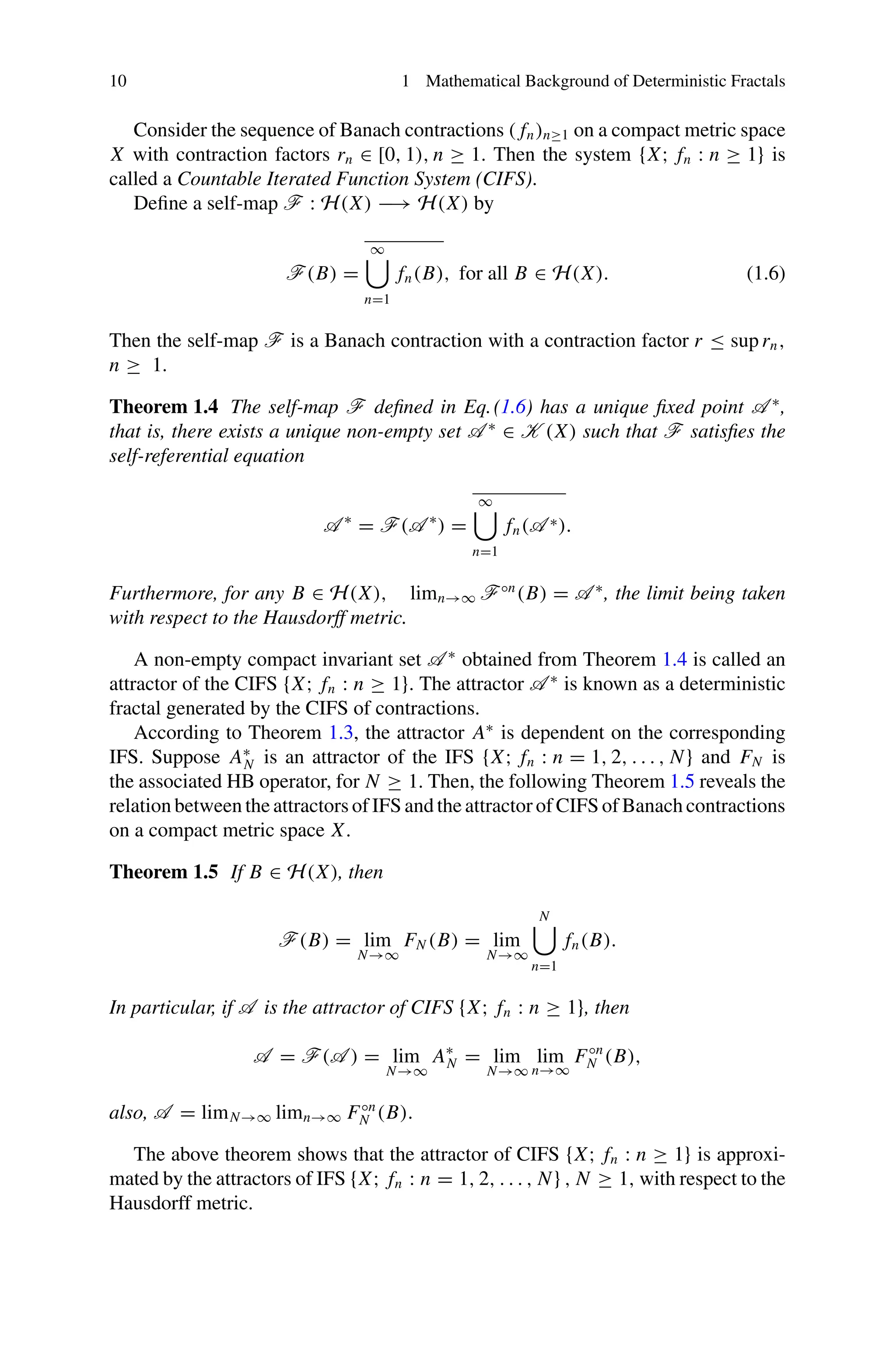
![1.3 Countable Iterated Function System 11
Example 1.1 Consider the space X = [0, 1] with the Euclidean metric. Let q ∈
(0, 1
2
], define fn : [0, 1] −→ [0, 1] by fn(x) = qn
x + αn, for all n ∈ N, where
α1 = 0 and αn = qn−1
+ 1−2q
2−3q
n−1
+ αn−1, n ≥ 2. Then the attractor of the CIFS
{X; fn : n ≥ 1} gives the infinite type Cantor set.
If q = 1/3 and αn = 1 − 1
3
n−1
, n ≥ 1, then the sequence of Banach contrac-
tions becomes fn = x
3n + 1 − 1
3n−1
, n ≥ 1.
Example 1.2 Let X = [0, 1] × [0, 1] ⊂ R2
, for every n = 4p + k, consider the fol-
lowing contractions:
fn(x, y) =
⎧
⎪
⎪
⎪
⎪
⎨
⎪
⎪
⎪
⎪
⎩
1
2p+1
1
3
x + 2p+1
− 2, 1
3
y , if k = 1,
1
2p+1
1
6
x −
√
3
6
y + 2p+1
− 5,
√
3
6
x + 1
6
y , if k = 2,
1
2p+1
1
6
x +
√
3
6
y + 2p+1
− 3
2
, −
√
3
6
x + 1
6
y +
√
3
6
, if k = 3,
1
2p+1
1
3
x + 2p+1
− 4
3
, 1
3
y , if k = 4.
Then the attractor of the CIFS {X; fn : n ≥ 1} gives the infinite type von Koch
curve.
1.4 Local Countable Iterated Function System
This section concisely provides the essential material of a local iterated function
system (LIFS) and describes the approximation process of the attractor of a local
countable iterated function system with the attractors of the iterated function system.
1.4.1 Local Iterated Function System
If {Xi : i ∈ Nn} is n number of non-empty subsets of X and for each Xi , there exists
a continuous mapping fi on Xi to X. Then the system {X; (Xi , fi ) : i ∈ N} is called
a local iterated function system (local IFS) [6] whereas, an iterated function system
(IFS) is a complete metric space X together with a finite set of contraction mappings,
denoted by {X; fk : k ∈ Nn}, with contraction factors ck, k ∈ Nn . If Xi = X, then
local IFS becomes (global) IFS. The operator Floc,n on H(X) is defined by
Floc,n(B) =
i∈Nn
fi (B ∩ Xi ).
Here fi (S ∩ Xi ) = { fi (x) : x ∈ S ∩ Xi }.](https://image.slidesharecdn.com/85835-250720042349-23fa1e14/75/Fractal-Functions-Dimensions-and-Signal-Analysis-Santo-Banerjee-25-2048.jpg)
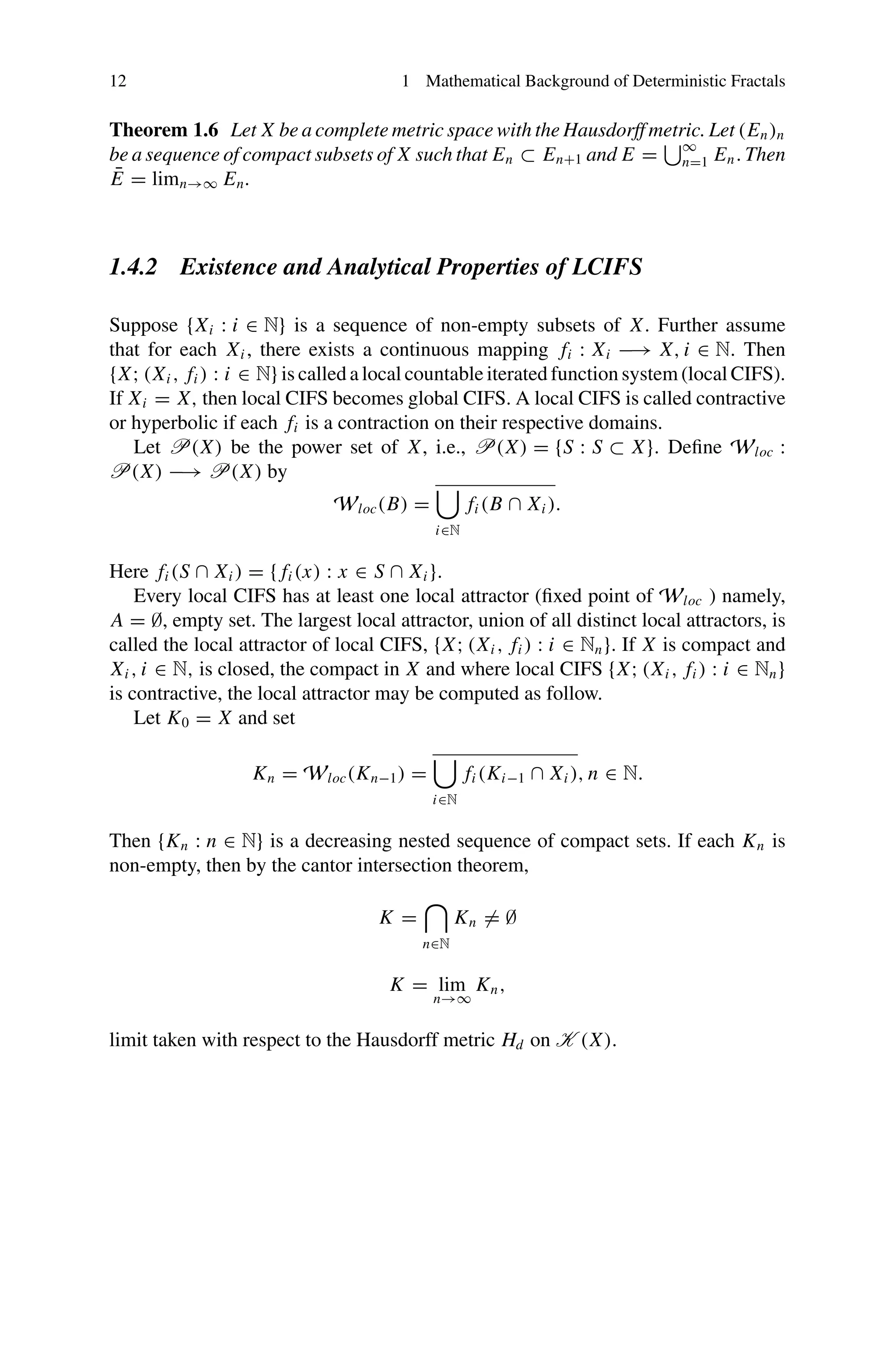
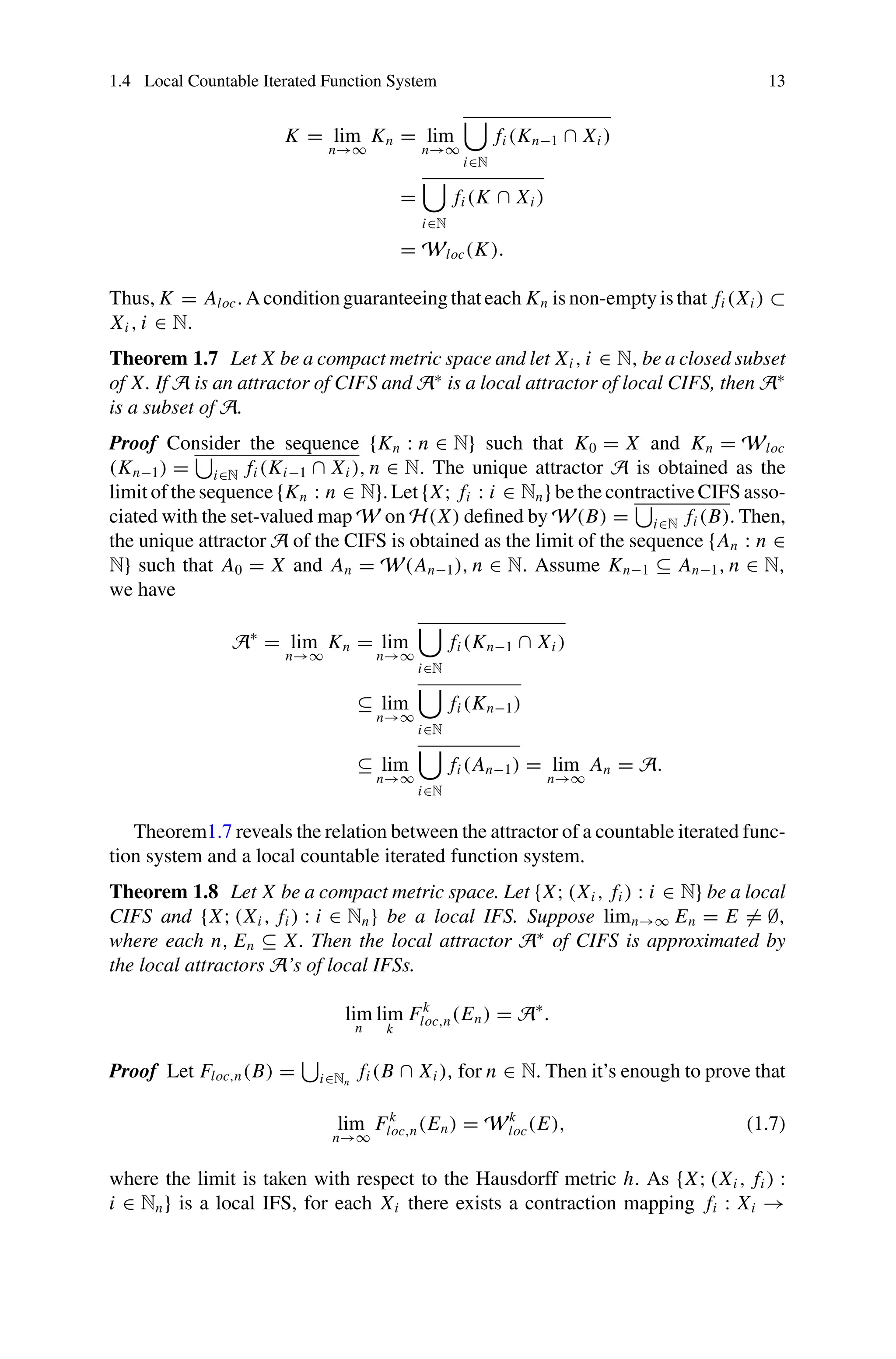
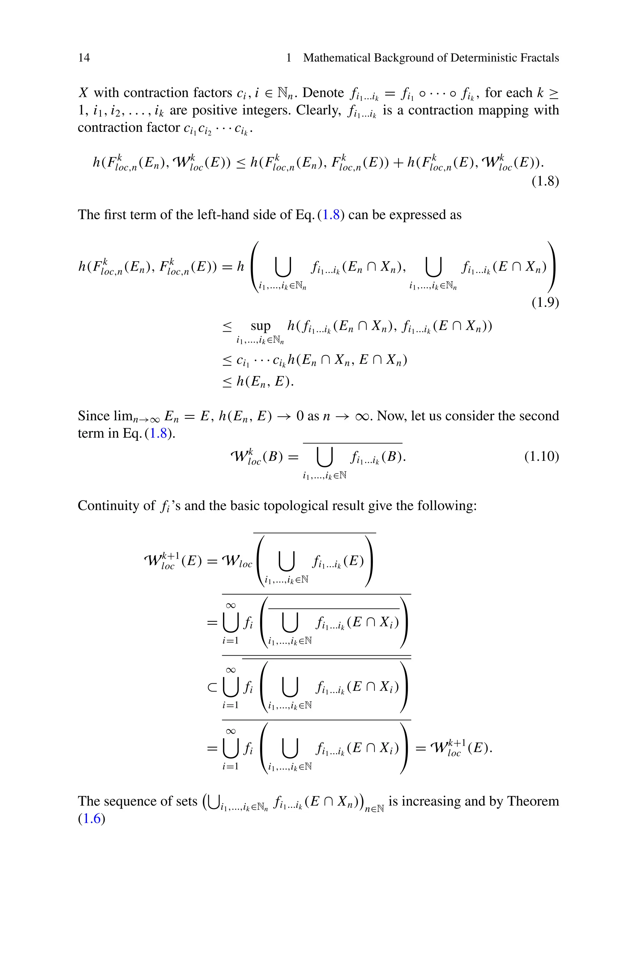
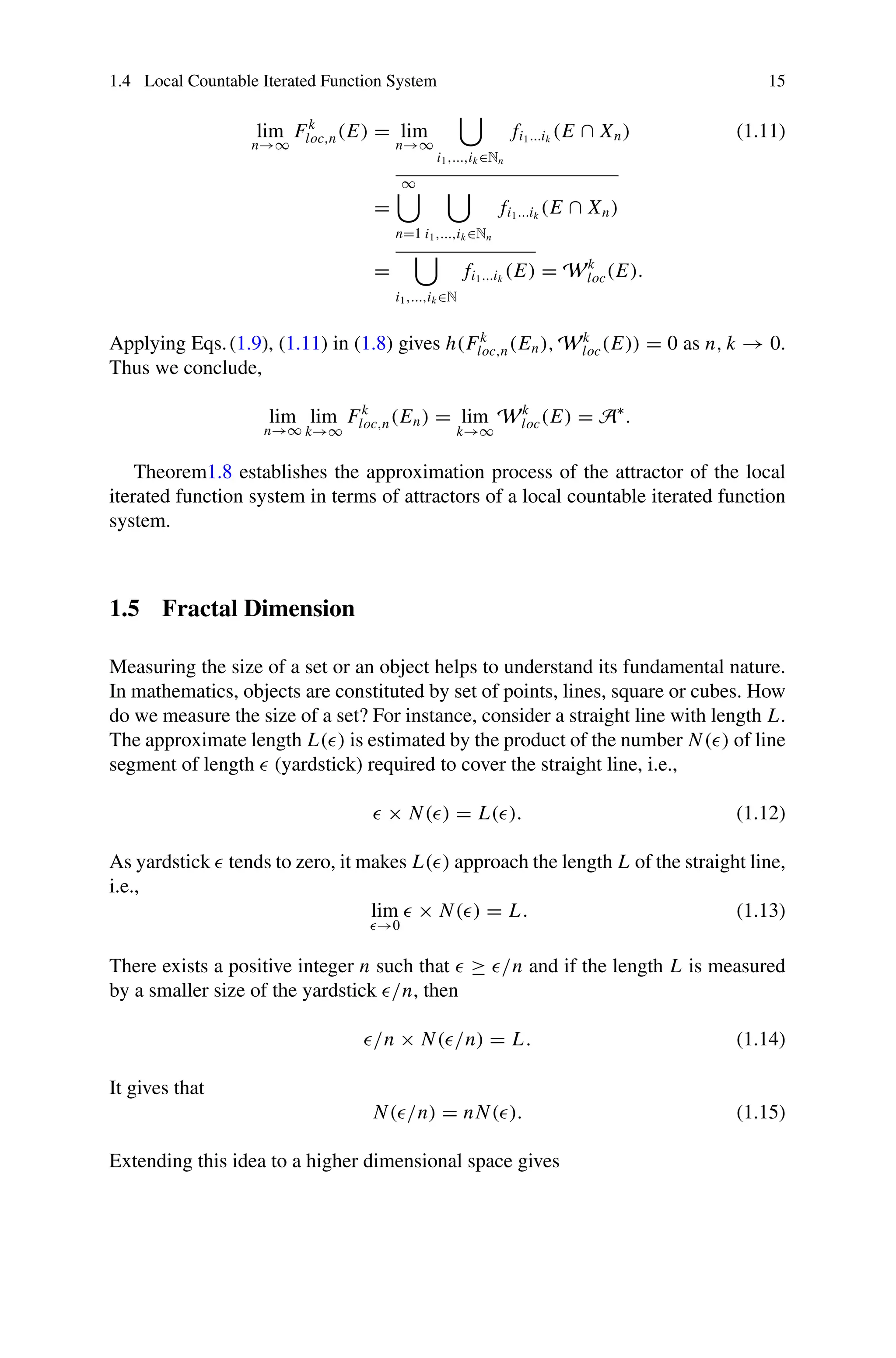
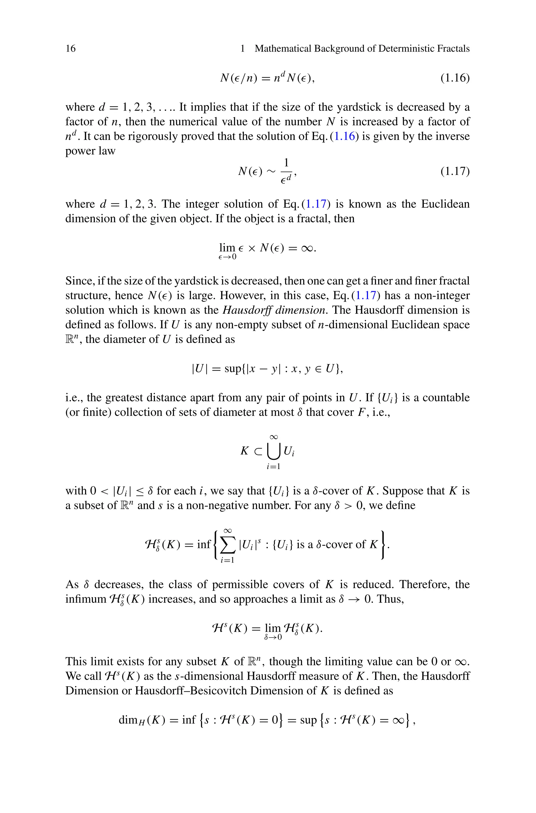
![1.5 Fractal Dimension 17
so that
Hs
(K) =
∞, if s dimH (K),
0, if s dimH (K).
If s = dimH (K), then Hs
(K) may be zero or infinite, or may be 0 Hs
(K) ∞.
The Hausdorff dimension has the advantage of being defined for any set, and is
mathematically convenient, as it is based on measures, which are relatively easy to
manipulate. The main disadvantage is that the explicit computation of the Hausdorff
dimension of a given set K is rather difficult since it involves taking the infimum
over covers consisting of balls of radius less than or equal to a given 0. A slight
simplification is obtained by considering only covers by the balls of radius equal to
. This gives rise to the concepts of the box dimension [8].
Let K ∈ H(X) and N() denote the smallest number of closed balls of radius
0 required to cover K. If
dimB = lim
→0
log N()
log(1/)
(1.18)
exists, then dimB is called the box dimension or fractal dimension of K.
Suppose that K is a subset in Rn
. The topological dimension of K, denoted as
dimT M, is inductively defined as follows:
1. dimT ∅ = −1,
2. The topological dimension of K at a point p ∈ K is less than or equal to n,
written as dim
p
T K ≤ n, if there exist arbitrarily small neighborhood of p whose
boundaries have a topological dimension at most n − 1,
3. K has a topological dimension at most n if it has a topological dimension at most
n at each of its points p:
dimT K ≤ n ⇐⇒ dim
p
T K ≤ n for all p ∈ K.
In addition, dim
p
T K = ∞, if condition (2) does not hold for any n ∈ N, and
dimT K = ∞ if condition (3) does not hold for any n ∈ N.
1.6 Generalized Fractal Dimensions
Fractal dimension is insufficient to characterize the object of interest having complex
and inhomogeneous scaling properties, since different irregular structures may have
the same fractal dimension [70, 71]. Thus, generalized fractal dimensions provide
more information about the space filling properties than the fractal dimension alone
(see, for instance, [1]). This section describes the generalized fractal dimensions
through Renyi entropy as follows.](https://image.slidesharecdn.com/85835-250720042349-23fa1e14/75/Fractal-Functions-Dimensions-and-Signal-Analysis-Santo-Banerjee-31-2048.jpg)
![18 1 Mathematical Background of Deterministic Fractals
Alfred Renyi introduced the measure to quantify the uncertainty or randomness
of a given system. It plays a vital role in the information theory [75].
Given probabilities pi ,
N
i=1 pi = 1, the Renyi entropy of order q is given by
REq =
1
1 − q
log
N
i=1
p
q
i ,
where q ≥ 0 and q = 1. At q = 1, the value of REq is potentially undefined as it
generates the indeterminate form, otherwise REq values are decreasing as a function
of q.
If q → 1, then REq → RE1 which is defined by
RE1 = −ln
N
i=1
pi log pi .
RE1 is called Shannon entropy. Renyi Fractal Dimensions or Generalized Fractal
Dimensions (GFD) of order q ∈ (−∞, ∞) are defined, in terms of generalized Renyi
Entropy, as
Dq = lim
r→0
1
q − 1
log2
N
i=1 p
q
i
log2 r
(1.19)
where pi is the probability distribution. For all q, we have Dq 0 and Dq is a
monotonically decreasing function of q such that D0 ≥ D1 ≥ D2. Also, observe that
Dq = D0 = 0, for all q for a constant signal because all probabilities except one
equal to zero, whereas the exceptional probability value is one.
1.6.1 Some Special Cases
• If q = 0, then
D0 =
log2 N
log2 r
, (1.20)
which is known as the Fractal Dimension.
• As q −→ 1, Dq converges to D1, which is given by
D1 = lim
r→0
N
i=1 pi log2 pi
log2 r
, (1.21)
where D1 is the Information Dimension
• If q = 2, then Dq is called the Correlation Dimension.](https://image.slidesharecdn.com/85835-250720042349-23fa1e14/75/Fractal-Functions-Dimensions-and-Signal-Analysis-Santo-Banerjee-32-2048.jpg)


![Jere., 210. Pond, John, 196. Pond. Joseph, 210. Pond, Joseph, 224.
Pond, Joshua, 50. Pond, Levi, 224. Pond, Mary, 203. Pond, Mel., 201.
Pond, Moses, 203. Pond, Moses, 206. Pond, Nathan, 208. Pond,
Nathan, Jun., 208. Pond, Gen' O., 210. Pond, Oliver, 201. Pond, Pallu,
211. Pond, Robert, 200. Pond, Robert, Jun., 200. Pond, Rub., 211.
Pond, Sam', 201. Pond, Seva, 126. Pond, Simeon, 150. Pond,
Stephen, 47. Pond, Timo., 211. Pond (Widow), 20O. Pond (Widow),
201. Pond, Zera, 29. Pormeman, Henry, 229. Pons, Thom, 190.
Ponton, Amariah, 230. Pooke, M', 184. Pooke, Will, 185. Pool Pool
Pool Pool Pool Pool Pool Pool Pool Poo] Pool Pool Pool Pool Pool Pool
Pool Pool Pool Pool Pool Pool Pool Pool Pool Pool Pool Pool Pool Pool
Pool Pool Pool Pool Pool Pool Pool Pool Poo! Poo: Pool Pool Pool Pool
Pool Pool Pool Pool Pool Pool Pool Pool Pool Pool Pool Abrahi, 70.
Akish, 39. Benj, 152. Benj, 164. Benj, 187. Caleb, 70, David, 70.
Ebenezer, 44. Ebenezer, 70. Ebenezer, Ju', 70, Edmund, 70.
Elizabeth, 69. Elliot, 44. Francis, 70. Hannah, 43. Hannah, 141.
Isaac, 43. Isaac, 70. Jacob, 44. Jacob, 164. Jacob, Ju', 165. James,
164. James, 219. John, 37. John, 70. John, 79. John, 169. John,
209. John, Ju', 70. John, 3'i, 70. Jon', 70. Jon, 151. Jon, J', 152.
Jon, 3i, 151. Joseph, 164. Joseph, Ju', 164. Joshua, 104. Mark, 70.
Moses, 70. Nathan, 70. Patience, 72. Polly, 160. Rufiis, 150. Sabinus,
57. Samuel, 165. Sarah, 165. Stephen, 70. Tho', 1.52. Tho., 210.
Tim, 151. William, 60. ,e, Abijah, 121. Jephthah, 121. e, Samuel,
121. er. Pharmi, 133. Poor, .braham, 64. Poor, Amos, 87. Poor,
.mo8, 87. Poor, .ndrew, 326. Poor, Benj, 64. Poor, Benj, 87. Poor,
Benj, 87. Poor, Benjn, 92. Poor, Benj, 118. Poor, Dani, 63. Poor,
Daniel, 63. Poor, Daniel, 92. Poor, Daniel. 93. Poor, David, 92. Poor,
David, 233. Poor, David, 244. Poor, Ebcn', 64. Poor, Enoch, 91. Poor,
Eunice, 225. Poor, Henry, 92. Poor, Jereniiah. 92. Poor, John, 64.
Poor, John, 74. Poor, John, 87. Poor, John, Ju', 64. Poor, Jonathan,
86. Poor, Joseph. 92. Poor, Mary, 64. Poor, Moses, 87. Poor, Moses,
92. Poor, Nathan, 88. Poor, Paul, 87. Poor, Peter, 64. Poor, Stephen,
86. Poor, Tho», 84. Poor, Timothy, 85. Poor, William, 91. Pope, Alice,
48. Pope, Ebenezer, 93. Pope, Eben', 191. Pope, Eben', 200. Pope,
Ebenezer, 237. Pope, Edmund, 48. Pope, Edward, 47. Pope, Elazer,
94. Pope, Eleazer, 69. Pope, Elijah, 09. Pope, Elijah, 199. Pope,](https://image.slidesharecdn.com/85835-250720042349-23fa1e14/75/Fractal-Functions-Dimensions-and-Signal-Analysis-Santo-Banerjee-48-2048.jpg)
![Prime (Negro), 38. Prime, Thomas, 92. Prince, .nne, 80. Prince,
Anno, SI. Prince. Brightenbury, 06. Prince. Daniel, 70. Prince, Daniel,
132. Prince, David, 40. Prince, David, 70. Prince, Ezekiel, 88. Prince,
Uannah, 66. Prince, Uenry, 97. Prince, James, 69. Prince, James, 89.
Prince, James, 176. . Prince, James, 189. Prince, James. Jun', 70.
Prince, Job, Jun', 189. Prince, John, 00. Prince, John. 81. Prince,
Joim, 94. Prince, John, 149. Prince, ]viml)al, 170. Prince, Lydia, 170.
Prmce, Molly, 80. Prmce (Negro), 36. Prince (Negro), 132. Prince,
Richard, 82. Prince, Richard, 95. Prmce, Samuel, 101. Prmce, Sam',
186. Prince, Stephen, 239. Prince, Thomas, 106. Prince, Thom', 190.
Prindle, Nathan, 119. Prindlev, Eldad, 72. Prindlev. Eliakim, 72.
Priutice, John. 235. Frintice, Samuel. 244. Printice, Thaddeus, 227.
Prior, Benj, 169. Prior, Ebenezer, 106. Prior, Eliphaz, 169. Prior, John,
116. Prior, Joseph. 169. Prior, Nathaniel. 50. Prior, Nathaniel. Jun',
50. Prior, Simeon, 119. Pritchard, Mrs., 194. Pritchard, M, 197.
Pritchard. The, 197. Pritchell. John, 82. Pritchet, Dorothy, 99.
Pritchet, Hugh. 90. Pritchett, Charity. 82. Pritchett, Joseph, 82.
Prockter, John, 75. Procter, Abel, 133. Procter, Benj'', 76. Procter,
Benj», 138. Procter, Eliz», 141. Procter, Gersliam. 141. Procter.
James, 158. Procter, John, 76. Procter, Jona, 141. Procter, Jon«, 161.
Procter, Joseph, 72. Procter, Joseph, 75. Procter, Mungo, 107.
Procter, Nath', 146. Procter, Nath, 150. Procter, Nathi, Jr., 146.
Procter, Oliver, Jn', 156. Procter, Peter, 126. Procter, Philip, 143.
Procter, Samuel. 48. Procter, Samuel, Jun', 48. Procter, Sarah , 75.
Procter, Simeon, 146. Procter, Simeon, Jur., 147. Proctor, Asa. 138.
Proctor, Azariah. 138. Proctor, Benjamin, 69. Proctor, Benjamin, Ju',
69. Proctor, Chas., 158. Proctor, Dan', 138. Proctor, Ebenez'. 94.
Proctor, Elm', 143. Proctor. Edward, 183. Proctor, Edwd. Jun', 184.
Proctor. Elijah, 138. Proctor, Elizabeth, 83. Proctor, Elizabeth, 83.
Proctor, Esther, 68. Proctor, Francis, 80. Proctor, Isaac, 72. Proctor,
Isaac, 80. Proctor, James, 84. Proctor, James, Jr., 158. Proctor,
Jeremiah, 83. Proctor, John, 69. Proctor, Johnson, 69. Proctor,
Jonathan, 69. Proctor, Jonathan, 82. Proctor, Joseph, 79. Proctor,
Joseph, 83. Proctor, Joseph, 84. Proctor, Levi, 139. Proctor,
Mehitable. 69. Proctor, Nathan, 09. Proctor. Nathan, 211. Proctor.
Nathan. Jun', 69. Proctor. Nicholas. 84. Proctor, Peter, 138. Proctor,](https://image.slidesharecdn.com/85835-250720042349-23fa1e14/75/Fractal-Functions-Dimensions-and-Signal-Analysis-Santo-Banerjee-52-2048.jpg)