This paper describes recent work by the IMF's European department to strengthen nowcasting capacity using novel data and modeling techniques. It compiles standard and non-traditional datasets like Google search and air quality for European economies. It applies dynamic factor models and machine learning algorithms to nowcast GDP growth, finding most methods outperform naive benchmarks. Dynamic factor models generally perform better in normal times while machine learning identifies turning points well. The scalable approach could be applied elsewhere subject to data availability.
![IMF WORKING PAPERS Nowcasting GDP: A Scalable Approach Using DFM, Machine Learning
and Novel Data, Applied to EuropeanEconomies
INTERNATIONAL MONETARY FUND 13
• Backtesting.In the firststage―to proxy a real-time environment―in each periodt,data on all
explanatory variables are available from the beginning of the sample till the latestquarter t. However,
information on the targetvariable is available only up to the t-1 quarter.In each quarter t, each model’s
parameters are estimated using data up to quarter t-1. Afterwards,the estimated models are applied to
explanatory variables in time tto produce a one-step-ahead out-of-sample prediction (pseudo
nowcast) of the targetvariable.Finally,forecasterrors are quantified by comparing actual and
estimated values of the targetvariable.
• Quantification ofindicators ofpredictive accuracy.In the second stage,using the forecasterrors from
backtesting,a number of differentstatistics can be quantified to assess how closely the forecasted
variable track the actual data.Since, each indicator have certain properties,e.g.,some may putmore
weighton outliers while others on main trends,we use the following statistics:
Rootmean squared error (RMSE):
𝑅𝑅𝑅𝑅𝑅𝑅𝑅𝑅 = �
∑ (𝑦𝑦𝑡𝑡 − 𝑦𝑦
�𝑡𝑡)2
𝑁𝑁
𝑡𝑡=1
𝑁𝑁
Mean absolute error (MAE):
𝑀𝑀𝑀𝑀𝑀𝑀 =
∑ 𝐴𝐴𝐴𝐴𝐴𝐴(𝑦𝑦𝑡𝑡 − 𝑦𝑦
�𝑡𝑡 )
𝑁𝑁
𝑡𝑡=1
𝑁𝑁
Mean Directional Accuracy (MDA):
𝑀𝑀𝑀𝑀𝑀𝑀 =
1
𝑁𝑁
∑1[𝑠𝑠𝑠𝑠𝑠𝑠(𝑦𝑦𝑡𝑡 − 𝑦𝑦𝑡𝑡−1) = 𝑠𝑠𝑠𝑠𝑠𝑠(𝑦𝑦
�𝑡𝑡 − 𝑦𝑦𝑡𝑡−1)],
where 1𝐴𝐴(x) = �
1 𝑖𝑖𝑖𝑖 𝑥𝑥 ∈ 𝐴𝐴
0 𝑖𝑖𝑖𝑖 𝑒𝑒𝑒𝑒𝑒𝑒𝑒𝑒
and 𝑠𝑠𝑠𝑠𝑠𝑠(x) = �
−1 𝑖𝑖𝑖𝑖 𝑥𝑥 < 0,
0 𝑖𝑖𝑖𝑖 𝑥𝑥 = 0,
1 𝑖𝑖𝑖𝑖 𝑥𝑥 > 0
The firsttwo indicators (RMSE and MAE) representmeasures of the average model prediction error.
By squaring the error terms,RMSE puts higher weights to large errors.It is a useful indicator to
compare predictive power of differentmodels particularly when large errors are present.While MAE is
only slightly differentin definition from the MSE,it has differentproperties as it assigns same weights
to both large and small errors.Thus,unlike the MSE, MAE is not putting too much weighton outliers
and it provides a generic measure of how well a model is performing.The MDA is a measure of
predictive accuracy thatindicates the probability with which a model forecastthe actual direction of a
time series.In other words,MDA compares the forecastdirection (upward or downward) to the actual
realized direction.
These statistics of predictive accuracynot only inform practitioners of how closely individual models
predict actual data but can also be used to derive weights when aggregating results from individual
models. For example,we have used the inverse RMSEs of each model as their weights to produce a weighted
average of their predictions.
A specific method may outperform others on a a particular data set,however,other methods may work
better on a different data set.3 Similarly―in the contextof nowcasting―a method may perform better during
specific episodes,i.e.,stable growth or a sharp contraction/revival in economic activity.As there is no criteria
for selecting a model a priori based on an individual country’s characteristics,selectinga proper method―for
any given set of data―that produces the bestresults is a critical step.To assess and compare the performance
3
Hastie (2009) or Gareth (2015) provide a more detailed discussion of this issue.](https://image.slidesharecdn.com/nowcastinggdp-scalableapproachusingdfmmachinelearning-240223233421-449afb13/75/Nowcasting-GDP-Scalable-Approach-Using-DFM-Machine-Learning-pdf-15-2048.jpg)
![IMF WORKING PAPERS Nowcasting GDP: A Scalable Approach Using DFM, Machine Learning
and Novel Data, Applied to EuropeanEconomies
INTERNATIONAL MONETARY FUND 18
Table 4. During COVID-19 Sample- Model Performance (RMSE) Between2020Q1-2021Q1
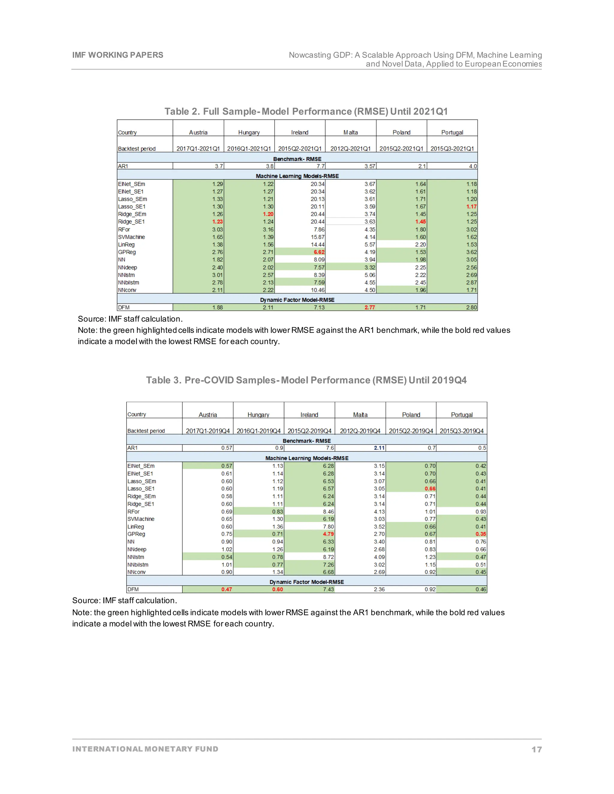
Source: IMF staff calculation.
Note: the green highlightedcells indicate models with lower RMSE against the AR1 benchmark, while the bold red values
indicate a model with the lowest RMSE for each country.
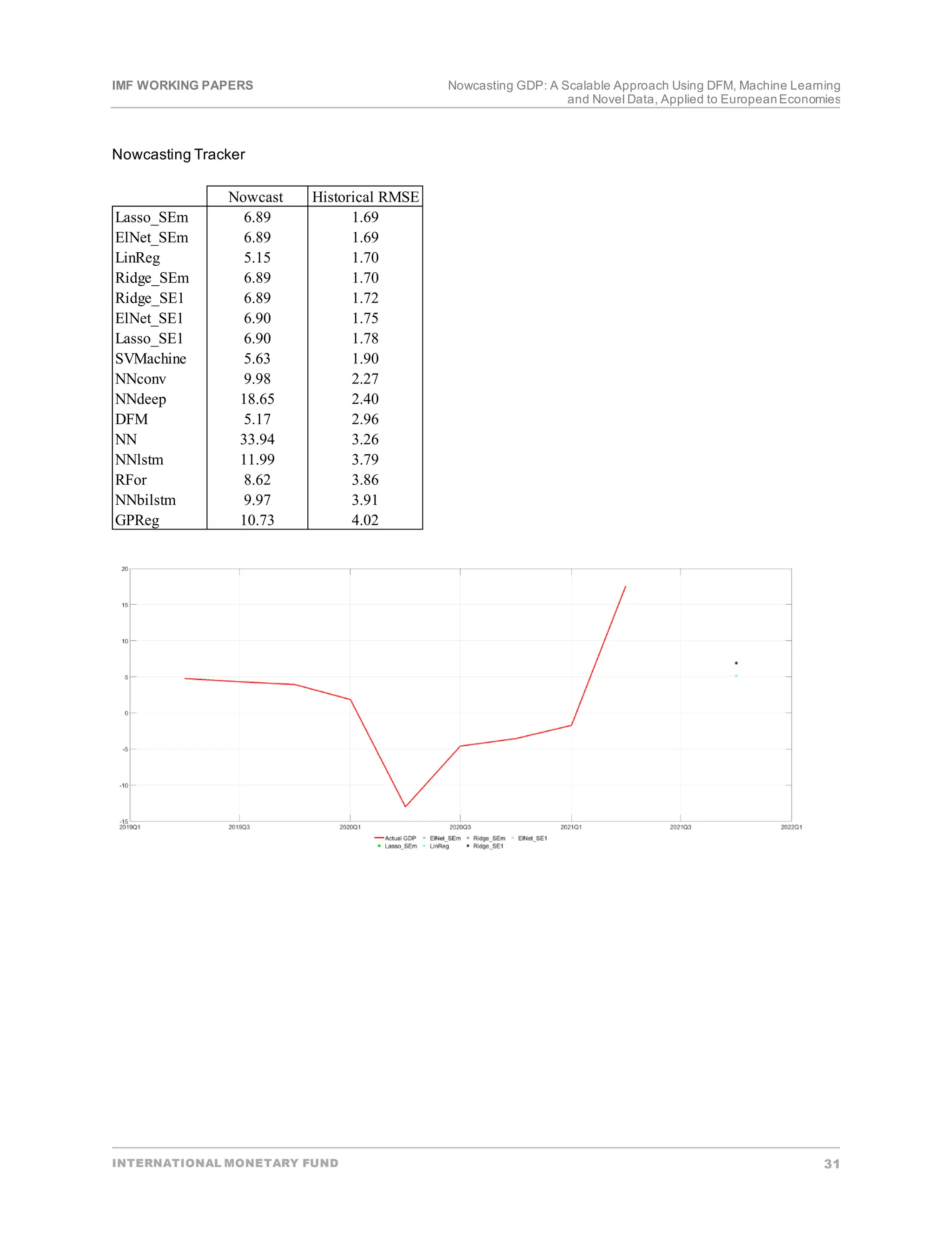
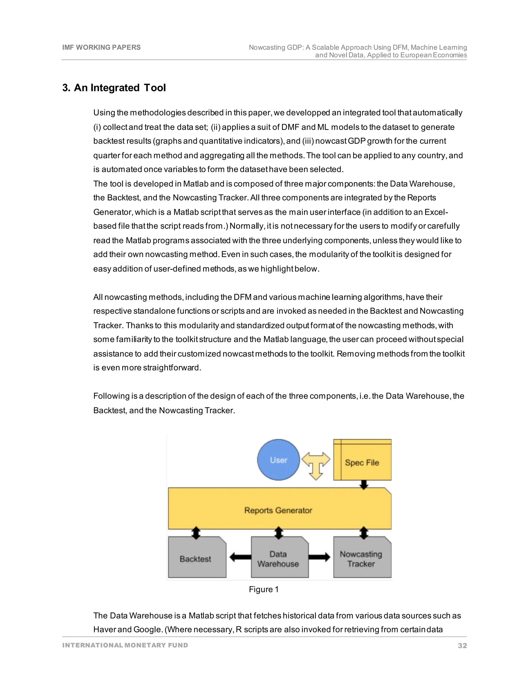
To operationalize our findings, we developed an integrated, fully-automated nowcasting tool. The tool
automatically (i) collects and treats the dataset; (ii) applies a suit of DFM and ML models to the datasetto
perform backtest(charts and indicators of forecasting accuracy);(iii) re-estimate the modeleach time new data
becomes available and produces a nowcastof the currentquarter GDP growth;and, (iv) generates an
aggregated outputfor all the methods across the whole period and the subsamples.Once variables to form the
datasethave been selected,the tool can be easily applied to any country,subjectto data availability
(Annex [2]).
Summary and Conclusion
The COVID-19 pandemic has underscoredthe need for timely data and methods, which allow for the
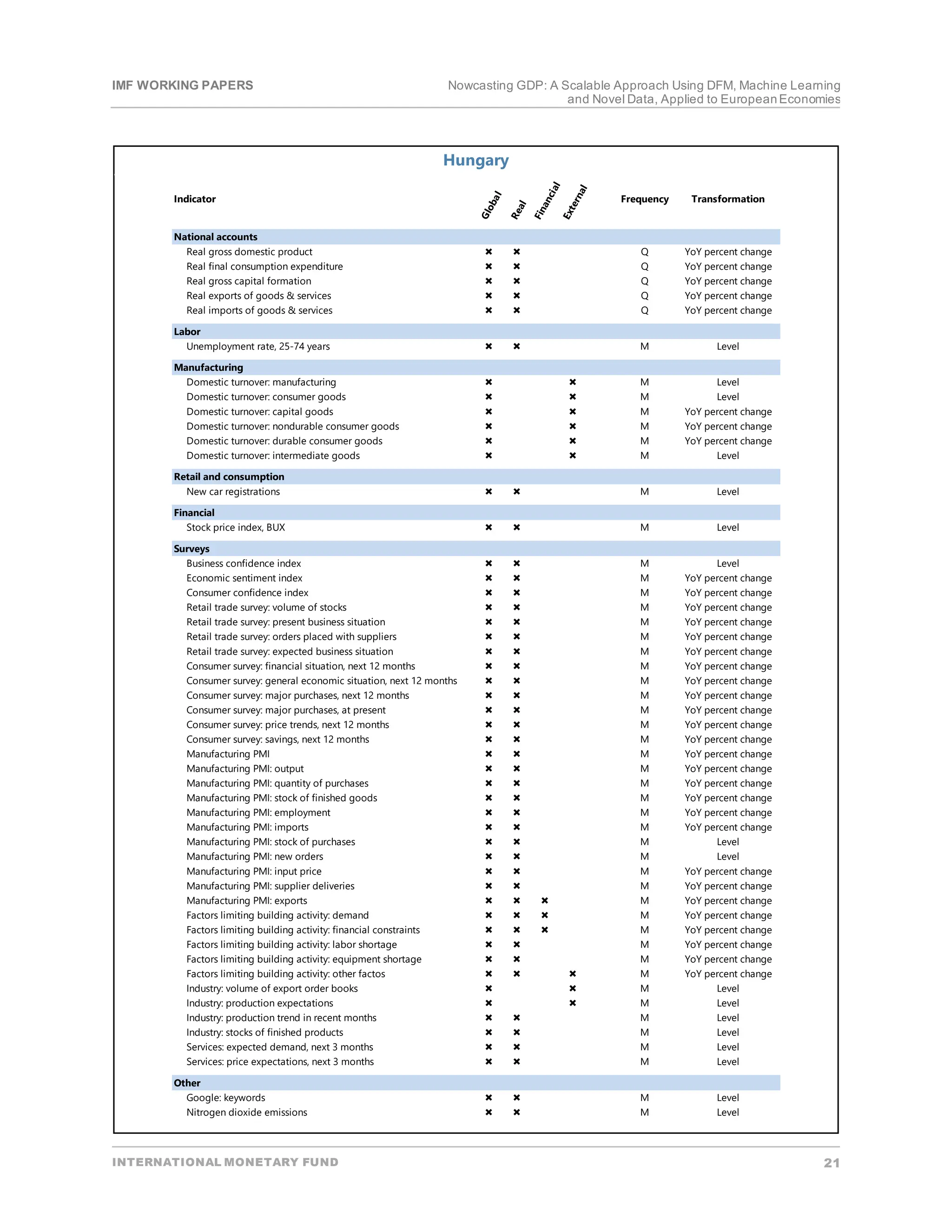
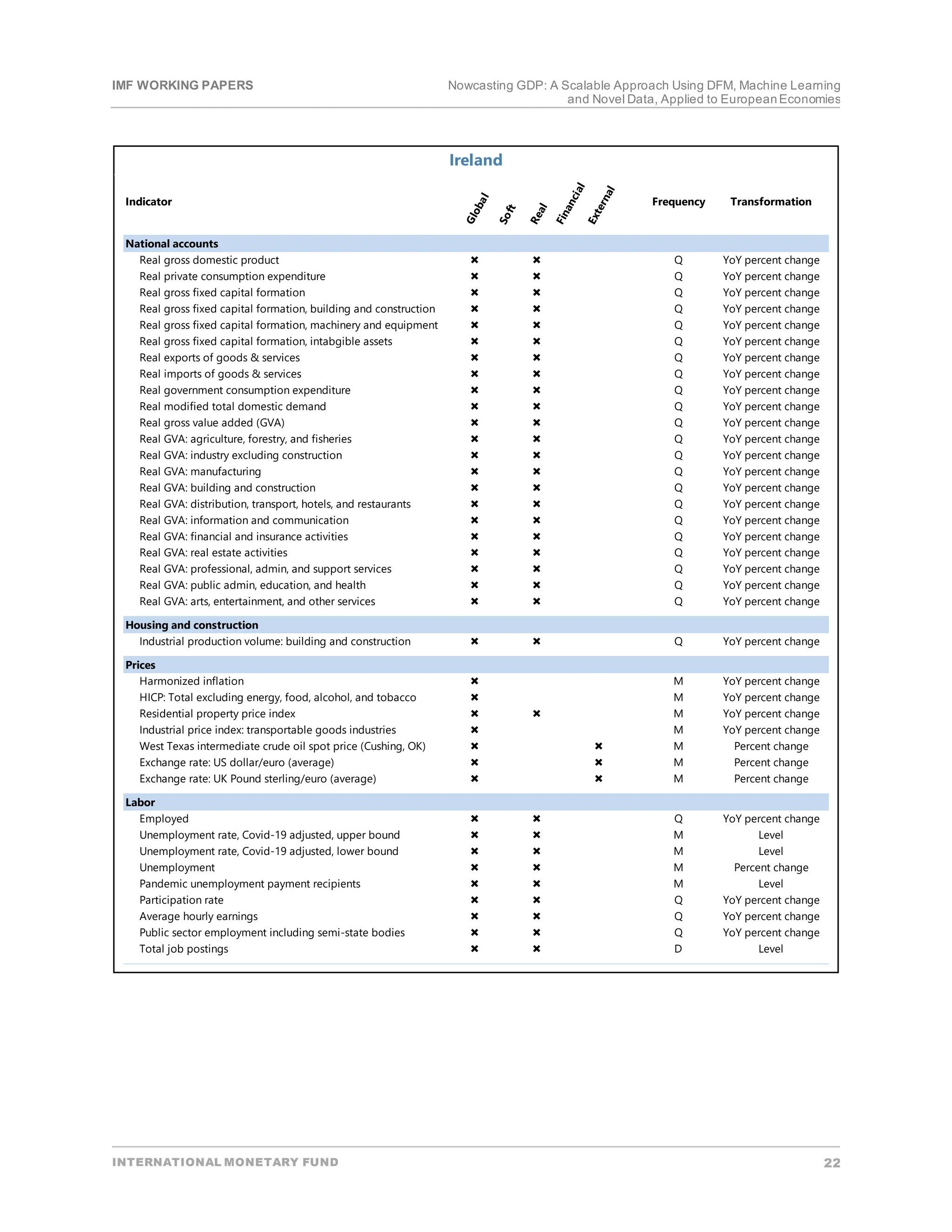
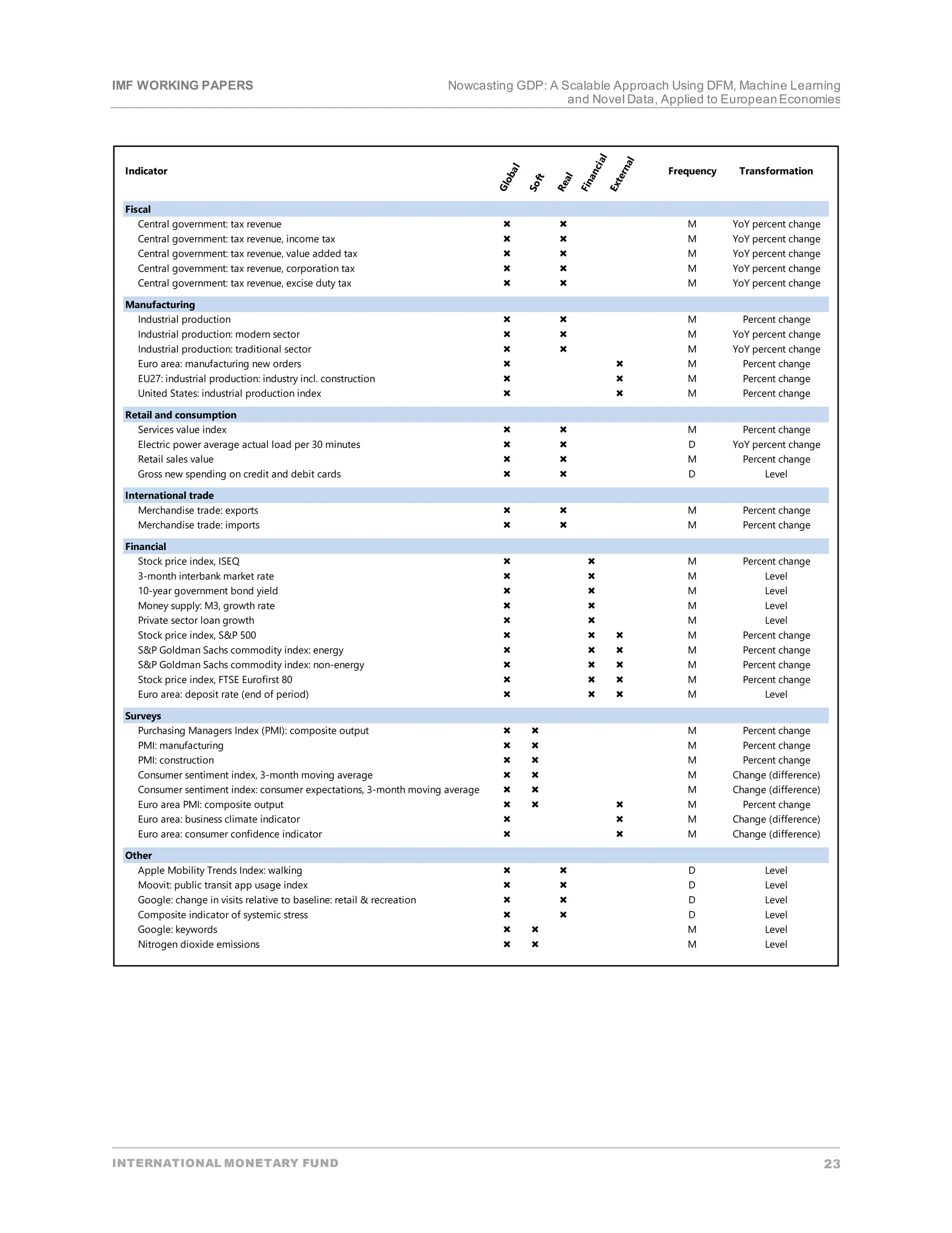
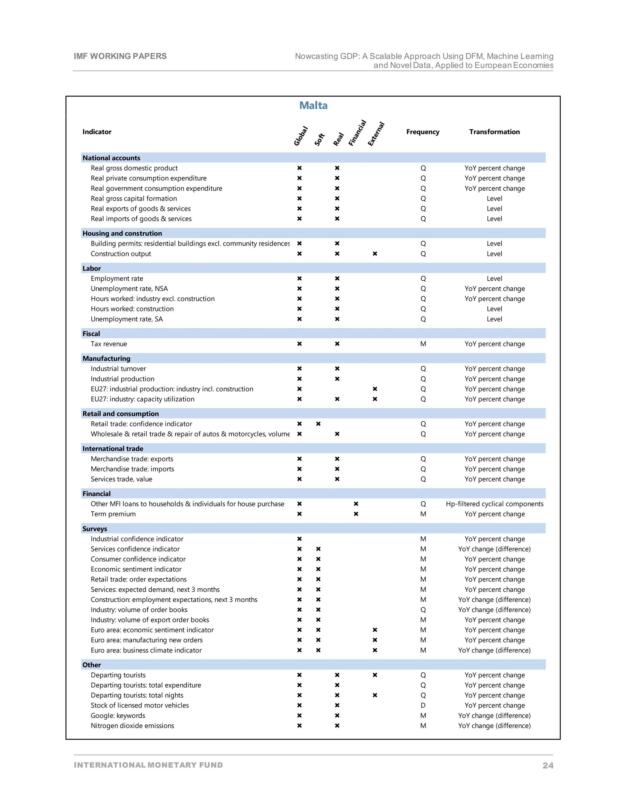
assessment of economies’current health. We motivate,compile,and discuss datasets for six European
economies and apply and compare traditional and new nowcasting methods for the period 1995Q1-2021Q4 as
well as during normal times (1995-2019) and during the COVID-19 pandemic (2020Q1 up to 2021q4).The
datasets comprise standard variables suggested by the literature as well as new variables thathave become
recently available such as Google Trends and air quality.We provide lists of variables,and their
transformations,for six European countries thatcan serve as examples for other economies.To avoid issues
linked to large datasets (collinearity between explanatory variables and model overfitting),we apply methods
capable of reducing the dimension of the original dataset.As a representative of a standard approach,we
apply a DFM following the New York Fed tradition.Building on the growing evidence of the usefulness of
machine learning methods in economics,we introduce several ML algorithms to our exercise.
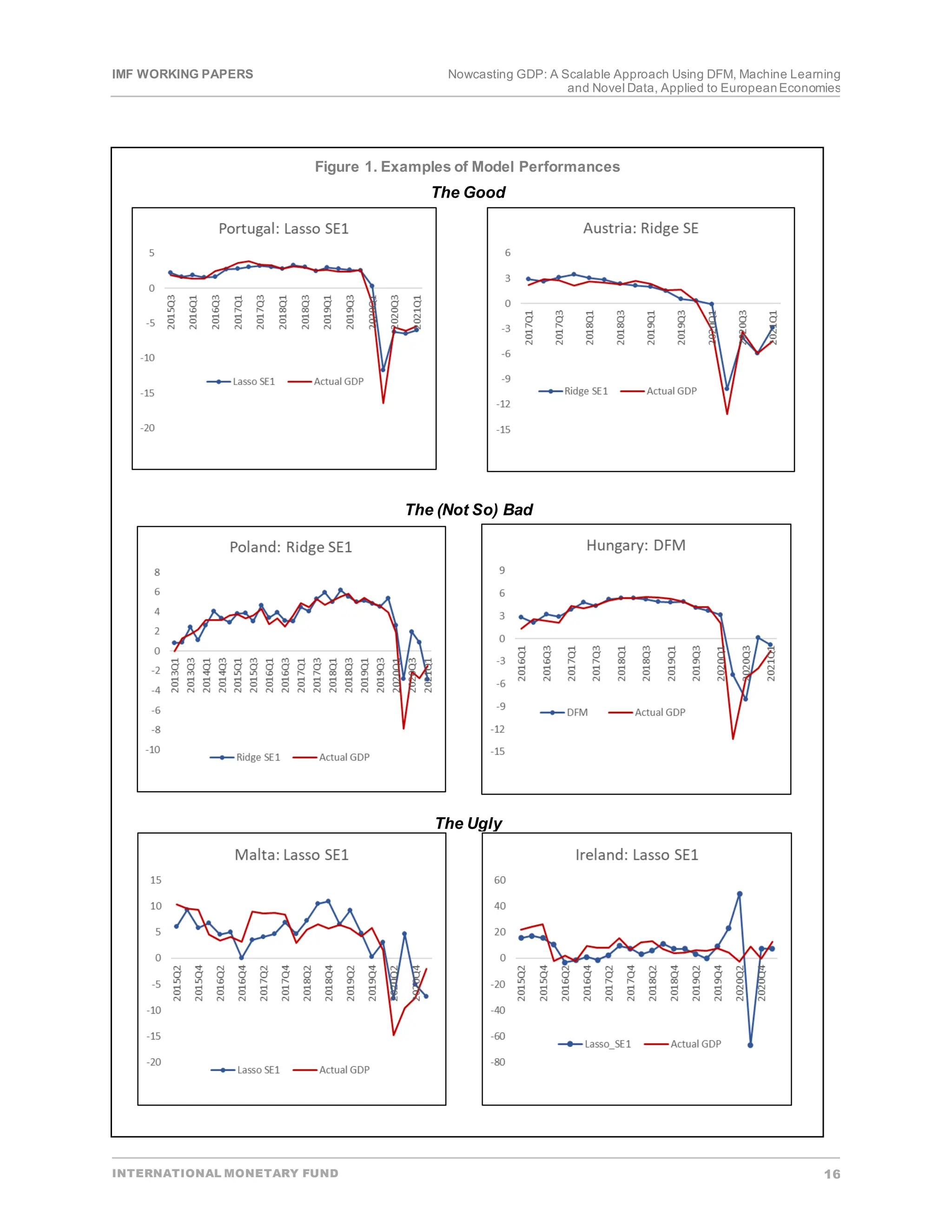
Overall, we find that the tools we applied add value and have the power to inform the nowcast of the
current quarter GDP growth. Applying alternative methods and comparing their predictive capability on
historical data,we find that a strong majority of our methods outperform the AR(1) benchmark model.
Specifically,applying the ML methods reduced the average forecasterrors up to 75 percentand the DFM
reduced the forecasterror by half compared to the AR(1) model across all countries.Nonetheless,we found](https://image.slidesharecdn.com/nowcastinggdp-scalableapproachusingdfmmachinelearning-240223233421-449afb13/75/Nowcasting-GDP-Scalable-Approach-Using-DFM-Machine-Learning-pdf-20-2048.jpg)
![IMF WORKING PAPERS Nowcasting GDP: A Scalable Approach Using DFM, Machine Learning
and Novel Data, Applied to EuropeanEconomies
INTERNATIONAL MONETARY FUND 35
Similar to linear regression,SVM is also a linear function in order to predictthe targetvariable 𝑦𝑦𝑡𝑡
𝑓𝑓(𝑥𝑥𝑡𝑡
) = 𝑥𝑥𝑡𝑡
′
𝛽𝛽 + 𝑏𝑏
Formally,SVM algorithm aims atfinding 𝑓𝑓(𝑥𝑥𝑡𝑡) as flatas possible while maintaining the forecasterror capped
within certain band.1 Thus,SVM will minimize its loss function by finding a combination of 𝛽𝛽 and observation-
specific positive slack constants 𝜉𝜉𝑡𝑡 and 𝜉𝜉𝑡𝑡
∗
:
1
2
𝛽𝛽′
𝛽𝛽 + 𝐶𝐶 �(𝜉𝜉𝑡𝑡 + 𝜉𝜉𝑡𝑡
∗
)
𝑇𝑇
𝑡𝑡=1
𝑠𝑠.𝑡𝑡. 𝑦𝑦𝑡𝑡 − 𝑓𝑓(𝑥𝑥𝑡𝑡
) ≤ 𝜀𝜀 + 𝜉𝜉𝑡𝑡
𝑓𝑓(𝑥𝑥𝑡𝑡 ) − 𝑦𝑦𝑡𝑡 ≤ 𝜀𝜀 + 𝜉𝜉𝑡𝑡
∗
Therefore,ateach point, the forecasterror is capped by [−𝜀𝜀, 𝜀𝜀], and can be relaxed by at most𝜉𝜉𝑡𝑡
∗
or 𝜉𝜉𝑡𝑡 at
higher or lower end.The constantC is the regularization hyperparameter and controls the trade-off between
minimizing errors and penalizing overfitting.If C = 0, the algorithm disregards individual deviations and
constructs the simplesthyperplane for which every observation is still within the acceptable margin of 𝜀𝜀.For
sufficiently largeC,the algorithm will constructthe mostcomplex hyperplane thatpredicts the outcome for the
training data with zero error (Bolhuis and Rayner 2020).
Chart[x]: A simple SVM to nowcastGDP
Note: The orange hyperplane is the prediction,while blue dots are actual observations.The model contains
40 regressors,while to visualize,we only use term premium and economic sentiment.
1
Bolhuis and Rayner (2020) define support vector machine(SVM) as an algorithm that constructs hyperplanes to partitionpredictor
combinations and make a point forecast for each of thesections.](https://image.slidesharecdn.com/nowcastinggdp-scalableapproachusingdfmmachinelearning-240223233421-449afb13/75/Nowcasting-GDP-Scalable-Approach-Using-DFM-Machine-Learning-pdf-37-2048.jpg)
![IMF WORKING PAPERS Nowcasting GDP: A Scalable Approach Using DFM, Machine Learning
and Novel Data, Applied to EuropeanEconomies
INTERNATIONAL MONETARY FUND 36
In practice,the constraintoptimization problem can be solved using Lagrange dual formulation.2 Introducing
nonnegative Lagrangian multipliers 𝛼𝛼𝑡𝑡 and 𝛼𝛼𝑡𝑡
∗
for each observation 𝑋𝑋𝑡𝑡,the dual Lagrangian is as follows:
𝐿𝐿(𝛼𝛼) =
1
2
� �(𝛼𝛼𝑖𝑖 − 𝛼𝛼𝑖𝑖
∗
)�𝛼𝛼𝑗𝑗 − 𝛼𝛼𝑗𝑗
∗
�𝑥𝑥𝑖𝑖
′
𝑥𝑥𝑗𝑗 +
𝑇𝑇
𝑗𝑗=1
𝑇𝑇
𝑖𝑖=1
𝜀𝜀 �(𝛼𝛼𝑖𝑖 + 𝛼𝛼𝑖𝑖
∗
) + � 𝑦𝑦𝑖𝑖(𝛼𝛼𝑖𝑖
∗
− 𝛼𝛼𝑖𝑖)
𝑇𝑇
𝑖𝑖=1
𝑇𝑇
𝑖𝑖=1
𝑠𝑠.𝑡𝑡. �(𝛼𝛼𝑡𝑡 − 𝛼𝛼𝑡𝑡
∗) = 0
𝑇𝑇
𝑡𝑡=1
∀𝑡𝑡: 0 ≤ 𝛼𝛼𝑡𝑡 ≤ 𝐶𝐶
∀𝑡𝑡: 0 ≤ 𝛼𝛼𝑡𝑡
∗
≤ 𝐶𝐶
Solving the problem,we obtain
𝛽𝛽 = �(𝛼𝛼𝑡𝑡 − 𝛼𝛼𝑡𝑡
∗
)𝑥𝑥𝑡𝑡
𝑇𝑇
𝑡𝑡=1
and consequently for each new observation 𝑥𝑥,the prediction will be
𝑓𝑓(𝑥𝑥) = ∑ (𝛼𝛼𝑡𝑡 − 𝛼𝛼𝑡𝑡
∗)(𝑥𝑥𝑡𝑡
′
𝑥𝑥) + 𝑏𝑏
𝑇𝑇
𝑡𝑡=1 .
Replacing the dot product𝑥𝑥𝑗𝑗
′
𝑥𝑥𝑘𝑘 by other kernel functions,SVM can be applied to non-linear problems.
3. Random Forest
A decision tree is a non-parametric approach thatin each step iteratively splits a sample into two groups
chosen by the algorithm to yield the largestreduction in the forecasterror of the variable of interest(Bolhuis
and Rayner (2020)),the so-called recursive partitioning.Regression tree is nonparametric regression method
that allows for prediction of continuous variables (Chart[x]).Random forest (RF) is an ensemble method based
on a large number of individual decision (regression) trees created from differentsamples.
2
More details can be found in Drucker and others (1997).](https://image.slidesharecdn.com/nowcastinggdp-scalableapproachusingdfmmachinelearning-240223233421-449afb13/75/Nowcasting-GDP-Scalable-Approach-Using-DFM-Machine-Learning-pdf-38-2048.jpg)
![IMF WORKING PAPERS Nowcasting GDP: A Scalable Approach Using DFM, Machine Learning
and Novel Data, Applied to EuropeanEconomies
INTERNATIONAL MONETARY FUND 37
Chart[x]: A simple regression tree to nowcastGDP
Note: each terminal node represents a region 𝑅𝑅𝑚𝑚.
A formal expression of a regression tree is
𝑓𝑓
̂(𝑥𝑥) = � 𝑐𝑐̂𝑚𝑚𝐼𝐼(𝑥𝑥 ∈ 𝑅𝑅𝑚𝑚)
𝑀𝑀
𝑚𝑚=1
where 𝐼𝐼(⋅) is the indicator function and 𝑐𝑐̂𝑚𝑚 = 𝑎𝑎𝑎𝑎𝑎𝑎(𝑦𝑦𝑖𝑖|𝑥𝑥𝑖𝑖 ∈ 𝑅𝑅𝑚𝑚),and 𝑅𝑅𝑚𝑚 is regions or the groups after iteratively
partitioned by the tree. The estimation then is seeking the optimized 𝑅𝑅𝑚𝑚 and 𝑐𝑐𝑚𝑚 to minimize the squared error:
min
{𝑅𝑅𝑚𝑚,𝑐𝑐𝑚𝑚}𝑚𝑚=1
𝑀𝑀
��𝑦𝑦𝑡𝑡 − 𝑓𝑓
̂(𝑥𝑥)�
2
A single regression tree tends to overfitdata butalso suffers from path dependence and model instability due
to its reliance on local rather than global optimization.These drawbacks have been addressed by RF. As an
ensemble method,RF uses the bootstrap aggregation (‘bagging’) to create a forestof individual trees,each of
which is estimated by a randomly chosen subsample of the observations as well as the predictors.For
regression tasks,the mean or average prediction of the individual trees is returned.](https://image.slidesharecdn.com/nowcastinggdp-scalableapproachusingdfmmachinelearning-240223233421-449afb13/75/Nowcasting-GDP-Scalable-Approach-Using-DFM-Machine-Learning-pdf-39-2048.jpg)
![IMF WORKING PAPERS Nowcasting GDP: A Scalable Approach Using DFM, Machine Learning
and Novel Data, Applied to EuropeanEconomies
INTERNATIONAL MONETARY FUND 38
4. NeuralNetwork
Neural network (NN) is a multi-layer non-linear method to map a series of inputs to a target output.Each layer
contains multiple nodes called artificial neurons. Each node receives inputs either from the inputdata matrix or
from nodes in previous layers and passes its outputeither to nodes in the next layer or as the final outputof the
model.Ateach node,a weighted sum of the inputs is transformed by a non-linear function 𝑓𝑓(⋅) to generate the
output. Typical functions used in neural networks include the rectified linear unit(ReLU) 𝑓𝑓(𝑧𝑧) = max(0,𝑧𝑧), as
well as hyperbolic tangent𝑓𝑓(𝑧𝑧) = (𝑒𝑒𝑧𝑧
− 𝑒𝑒−𝑧𝑧
)/(𝑒𝑒𝑧𝑧
+ 𝑒𝑒−𝑧𝑧
) or logistic function 𝑓𝑓(𝑧𝑧) = 1/(1 + 𝑒𝑒−𝑧𝑧
).
Given the structure of a NN,there is no closed form solution thatcould be estimated.Instead,NN is trained
using stochastic gradientdescentmethod,which (i) generates random weights,(ii) calculates the loss function
between the target variable and the outputpredicted based on these random weights,and (iii) minimizes the
loss function by adjusting weights with calculated gradients (LeCun Bengioand Hinton 2015).
Chart[x]: A simple neural network to nowcastGDP
Note: Each node represents a function 𝑓𝑓(⋅) transforming inputs to outputs.Each link represents the
weight,while black line means positive weight,gray line means negative weight.
In a standard setting,NN is feedforward and fully connected,meaning thatoutputfrom a specific node of each
layer will flow unidirectionally to all other the nodes in the nextlayer. Given the high flexibility in designing
and/or adding layers,several popular variations of NN are also introduced in our toolkit:
• The long short-term memory (LSTM) is a subtype of the larger class recursive neural networks (RNN),
which adds feedback connections in addition to the feedforward connections in classical NN.Such
modification makes LSTM more suitablefor time series prediction.](https://image.slidesharecdn.com/nowcastinggdp-scalableapproachusingdfmmachinelearning-240223233421-449afb13/75/Nowcasting-GDP-Scalable-Approach-Using-DFM-Machine-Learning-pdf-40-2048.jpg)