Download as PDF, PPTX


![SEMANTIC SEGMENTATION OF IMAGES USING DEEP
CONVOLUTIONAL NEURAL NETWORKS
(pixel level segmentation)
Novi Sad, October 2018
dr Velibor Ilić
RT RK Automotive
[Novi Sad AI] #3.0 - Deep Learning in Automotive Industry](https://image.slidesharecdn.com/novisadai-event3-2018-181101220312/85/Novi-sad-ai-event-3-2018-6-320.jpg)

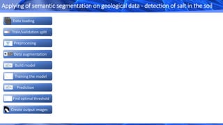
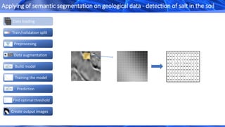
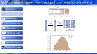
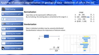
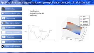
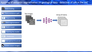
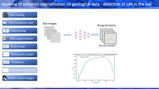
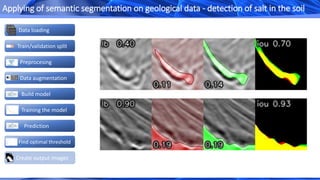
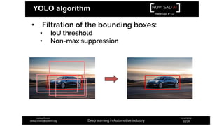
![Create output images
Data loading
Train/validation split
Data augmentation
Build model
Preprocesing
Prediction
Find optimal threshold
Training the model
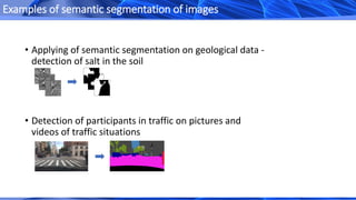
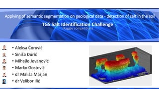
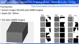
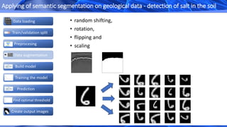
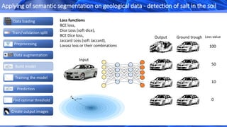
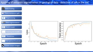
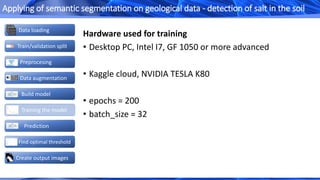
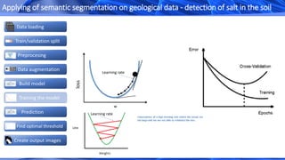
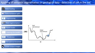
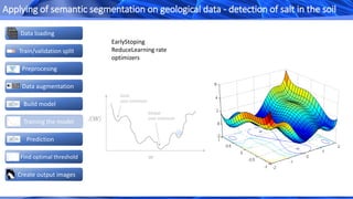
Applying of semantic segmentation on geological data - detection of salt in the soil
Total params: 5,119,857
Trainable params: 5,112,497
Non-trainable params: 7,360
# 101 -> 50
# 50 -> 25
# 25 -> 12
# 12 -> 6
# Middle 6 -> 3
# 6 -> 12
# 12 -> 25
# 25 -> 50
# 50 -> 101
deconv3 = Conv2DTranspose(start_neurons * 4, (3, 3), strides=(2, 2), padding="valid")(uconv4)
uconv3 = concatenate([deconv3, conv3])
uconv3 = Dropout(DropoutRatio)(uconv3)
uconv3 = Conv2D(start_neurons * 4, (3, 3), activation=None, padding="same")(uconv3)
uconv3 = residual_block(uconv3,start_neurons * 4)
uconv3 = residual_block(uconv3,start_neurons * 4, True)
conv1 = Conv2D(start_neurons * 1, (3, 3), activation=None, padding="same")(input_layer)
conv1 = residual_block(conv1,start_neurons * 1)
conv1 = residual_block(conv1,start_neurons * 1, True)
pool1 = MaxPooling2D((2, 2))(conv1)
pool1 = Dropout(DropoutRatio/2)(pool1)
Convolution
Deconvolution](https://image.slidesharecdn.com/novisadai-event3-2018-181101220312/85/Novi-sad-ai-event-3-2018-36-320.jpg)
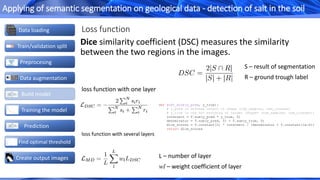
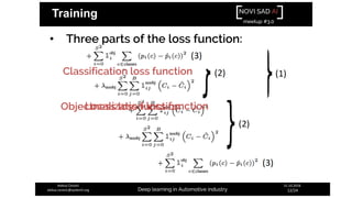
![p – result of segmentation
r – ground trought label
def cross_entropy(X,y):
# X is the output from fully connected layer .
(num_examples x num_classes)
# y is labels (num_examples x 1)
r = y.shape[0]
p = softmax(X)
log_likelihood = -np.log(p[range(m),y])
loss = np.sum(log_likelihood) / r
return loss
H(y,p)=−∑iyilog(pi)
Loss function
Weighted cross-entropy (WCE) can be expressed by the
following formula
Create output images
Data loading
Train/validation split
Data augmentation
Build model
Preprocesing
Prediction
Find optimal threshold
Training the model
Applying of semantic segmentation on geological data - detection of salt in the soil](https://image.slidesharecdn.com/novisadai-event3-2018-181101220312/85/Novi-sad-ai-event-3-2018-38-320.jpg)


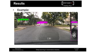
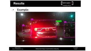


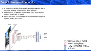
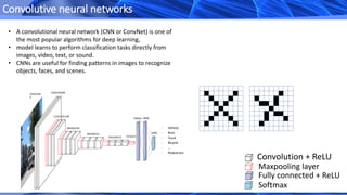
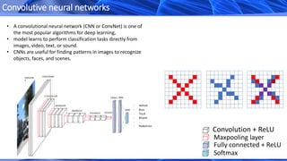
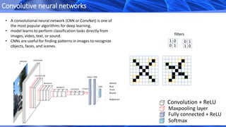
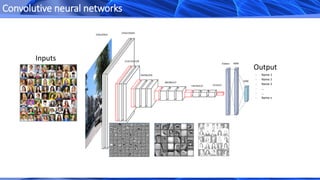
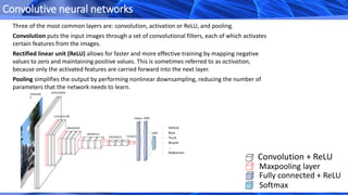
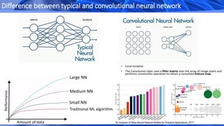
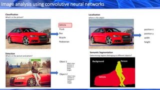
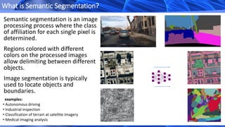
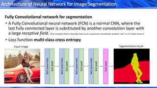
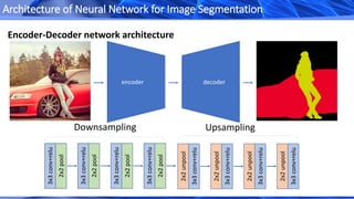
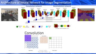
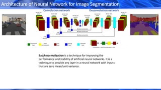
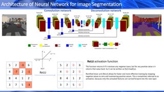
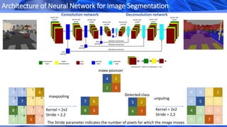
The document discusses semantic segmentation of images using deep convolutional neural networks. It provides examples of semantic segmentation applied to geological data to detect salt in soil and detecting traffic participants in photos and videos. It also outlines the architecture of neural networks used for image segmentation, including fully convolutional networks and encoder-decoder networks. Components like convolution layers, ReLU activation, batch normalization, max pooling, and upsampling are described.