19.2
19-1 IPv4 ADDRESSES
19-1IPv4 ADDRESSES
An
An IPv4 address
IPv4 address is a
is a 32-bit
32-bit address that uniquely and
address that uniquely and
universally defines the connection of a device (for
universally defines the connection of a device (for
example, a computer or a router) to the Internet.
example, a computer or a router) to the Internet.
Address Space
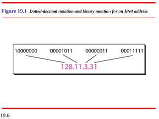
Notations
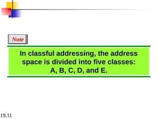
Classful Addressing
Classless Addressing
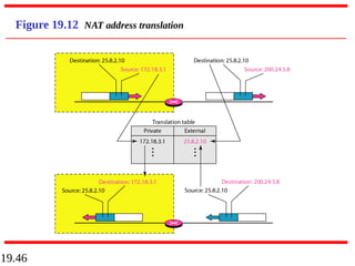
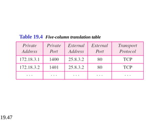
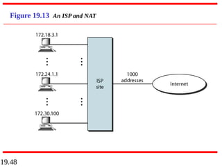
Network Address Translation (NAT)
Topics discussed in this section:
Topics discussed in this section:
19.8
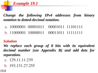
Change the followingIPv4 addresses from binary
notation to dotted-decimal notation.
Example 19.1
Solution
We replace each group of 8 bits with its equivalent
decimal number (see Appendix B) and add dots for
separation.
9.
19.9
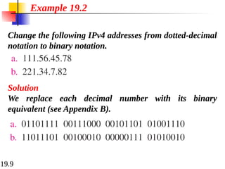
Change the followingIPv4 addresses from dotted-decimal
notation to binary notation.
Example 19.2
Solution
We replace each decimal number with its binary
equivalent (see Appendix B).
10.
19.10
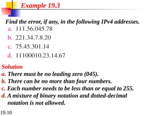
Find the error,if any, in the following IPv4 addresses.
Example 19.3
Solution
a. There must be no leading zero (045).
b. There can be no more than four numbers.
c. Each number needs to be less than or equal to 255.
d. A mixture of binary notation and dotted-decimal
notation is not allowed.
19.13
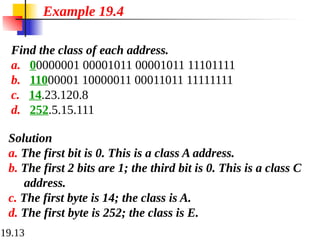
Find the classof each address.
a. 00000001 00001011 00001011 11101111
b. 11000001 10000011 00011011 11111111
c. 14.23.120.8
d. 252.5.15.111
Example 19.4
Solution
a. The first bit is 0. This is a class A address.
b. The first 2 bits are 1; the third bit is 0. This is a class C
address.
c. The first byte is 14; the class is A.
d. The first byte is 252; the class is E.
19.18
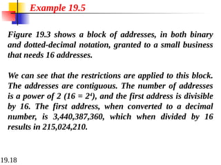
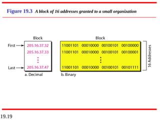
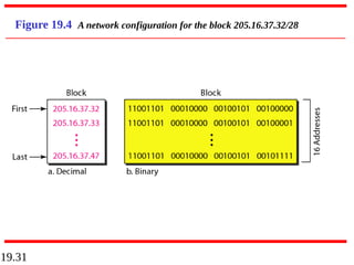
Figure 19.3 showsa block of addresses, in both binary
and dotted-decimal notation, granted to a small business
that needs 16 addresses.
We can see that the restrictions are applied to this block.
The addresses are contiguous. The number of addresses
is a power of 2 (16 = 24
), and the first address is divisible
by 16. The first address, when converted to a decimal
number, is 3,440,387,360, which when divided by 16
results in 215,024,210.
Example 19.5
19.20
In IPv4 addressing,a block of
addresses can be defined as
x.y.z.t /n
in which x.y.z.t defines one of the
addresses and the /n defines the mask.
Note
21.
19.21
The first addressin the block can be
found by setting the rightmost
32 − n bits to 0s.
Note
22.
19.22
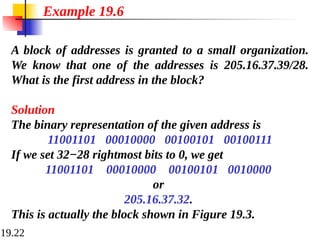
A block ofaddresses is granted to a small organization.
We know that one of the addresses is 205.16.37.39/28.
What is the first address in the block?
Solution
The binary representation of the given address is
11001101 00010000 00100101 00100111
If we set 32−28 rightmost bits to 0, we get
11001101 00010000 00100101 0010000
or
205.16.37.32.
This is actually the block shown in Figure 19.3.
Example 19.6
23.
19.23
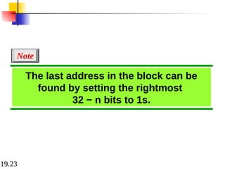
The last addressin the block can be
found by setting the rightmost
32 − n bits to 1s.
Note
24.
19.24
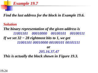
Find the lastaddress for the block in Example 19.6.
Solution
The binary representation of the given address is
11001101 00010000 00100101 00100111
If we set 32 − 28 rightmost bits to 1, we get
11001101 00010000 00100101 00101111
or
205.16.37.47
This is actually the block shown in Figure 19.3.
Example 19.7
25.
19.25
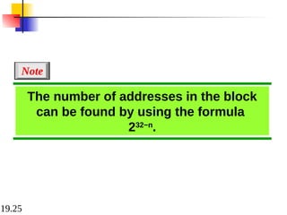
The number ofaddresses in the block
can be found by using the formula
232−n
.
Note
26.
19.26
Find the numberof addresses in Example 19.6.
Example 19.8
Solution
The value of n is 28, which means that number
of addresses is 2 32−28
or 16.
27.
19.27
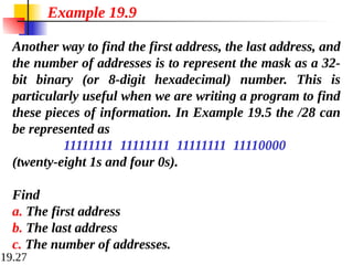
Another way tofind the first address, the last address, and
the number of addresses is to represent the mask as a 32-
bit binary (or 8-digit hexadecimal) number. This is
particularly useful when we are writing a program to find
these pieces of information. In Example 19.5 the /28 can
be represented as
11111111 11111111 11111111 11110000
(twenty-eight 1s and four 0s).
Find
a. The first address
b. The last address
c. The number of addresses.
Example 19.9
28.
19.28
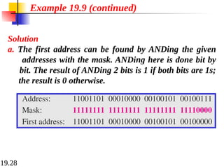
Solution
a. The firstaddress can be found by ANDing the given
addresses with the mask. ANDing here is done bit by
bit. The result of ANDing 2 bits is 1 if both bits are 1s;
the result is 0 otherwise.
Example 19.9 (continued)
29.
19.29
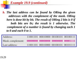
b. The lastaddress can be found by ORing the given
addresses with the complement of the mask. ORing
here is done bit by bit. The result of ORing 2 bits is 0 if
both bits are 0s; the result is 1 otherwise. The
complement of a number is found by changing each 1
to 0 and each 0 to 1.
Example 19.9 (continued)
30.
19.30
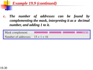
c. The numberof addresses can be found by
complementing the mask, interpreting it as a decimal
number, and adding 1 to it.
Example 19.9 (continued)
19.32
The first addressin a block is
normally not assigned to any device;
it is used as the network address that
represents the organization
to the rest of the world.
Note
19.35
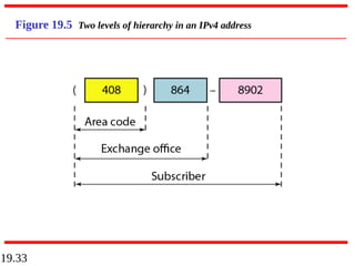
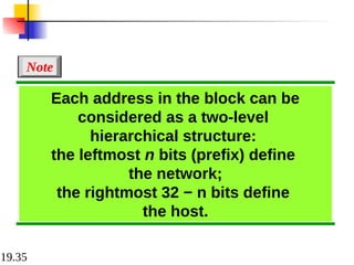
Each address inthe block can be
considered as a two-level
hierarchical structure:
the leftmost n bits (prefix) define
the network;
the rightmost 32 − n bits define
the host.
Note
19.38
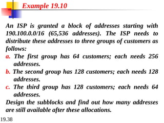
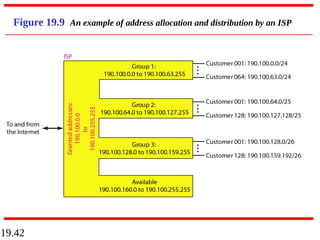
An ISP isgranted a block of addresses starting with
190.100.0.0/16 (65,536 addresses). The ISP needs to
distribute these addresses to three groups of customers as
follows:
a. The first group has 64 customers; each needs 256
addresses.
b. The second group has 128 customers; each needs 128
addresses.
c. The third group has 128 customers; each needs 64
addresses.
Design the subblocks and find out how many addresses
are still available after these allocations.
Example 19.10
39.
19.39
Solution
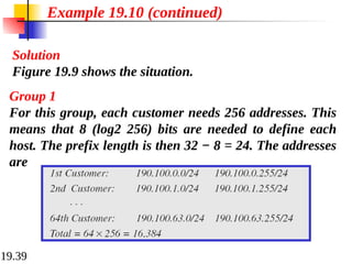
Figure 19.9 showsthe situation.
Example 19.10 (continued)
Group 1
For this group, each customer needs 256 addresses. This
means that 8 (log2 256) bits are needed to define each
host. The prefix length is then 32 − 8 = 24. The addresses
are
40.
19.40
Example 19.10 (continued)
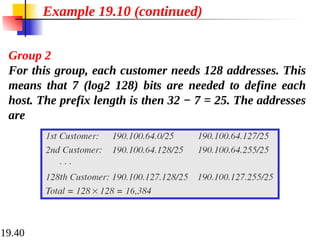
Group2
For this group, each customer needs 128 addresses. This
means that 7 (log2 128) bits are needed to define each
host. The prefix length is then 32 − 7 = 25. The addresses
are
41.
19.41
Example 19.10 (continued)
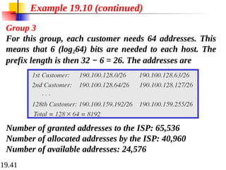
Group3
For this group, each customer needs 64 addresses. This
means that 6 (log264) bits are needed to each host. The
prefix length is then 32 − 6 = 26. The addresses are
Number of granted addresses to the ISP: 65,536
Number of allocated addresses by the ISP: 40,960
Number of available addresses: 24,576
19.49
19-2 IPv6 ADDRESSES
19-2IPv6 ADDRESSES
Despite all short-term solutions, address depletion is
Despite all short-term solutions, address depletion is
still a long-term problem for the Internet. This and
still a long-term problem for the Internet. This and
other problems in the IP protocol itself have been the
other problems in the IP protocol itself have been the
motivation for IPv6.
motivation for IPv6.
Structure
Address Space
Topics discussed in this section:
Topics discussed in this section:
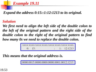
19.53
Expand the address0:15::1:12:1213 to its original.
Example 19.11
Solution
We first need to align the left side of the double colon to
the left of the original pattern and the right side of the
double colon to the right of the original pattern to find
how many 0s we need to replace the double colon.
This means that the original address is.
20.2
20-1 INTERNETWORKING
20-1 INTERNETWORKING
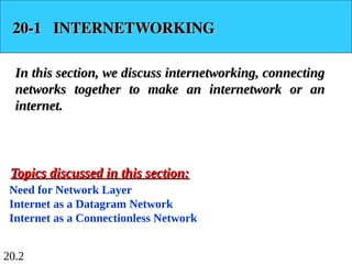
Inthis section, we discuss internetworking, connecting
In this section, we discuss internetworking, connecting
networks together to make an internetwork or an
networks together to make an internetwork or an
internet.
internet.
Need for Network Layer
Internet as a Datagram Network
Internet as a Connectionless Network
Topics discussed in this section:
Topics discussed in this section:
20.9
20-2 IPv4
20-2 IPv4
TheInternet Protocol version 4 (
The Internet Protocol version 4 (IPv4
IPv4) is the delivery
) is the delivery
mechanism used by the TCP/IP protocols.
mechanism used by the TCP/IP protocols.
Datagram
Fragmentation
Checksum
Options
Topics discussed in this section:
Topics discussed in this section:
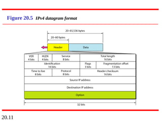
20.21
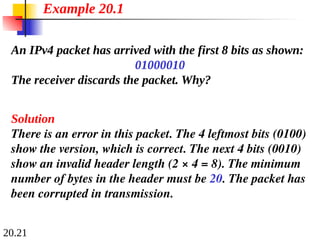
An IPv4 packethas arrived with the first 8 bits as shown:
01000010
The receiver discards the packet. Why?
Solution
There is an error in this packet. The 4 leftmost bits (0100)
show the version, which is correct. The next 4 bits (0010)
show an invalid header length (2 × 4 = 8). The minimum
number of bytes in the header must be 20. The packet has
been corrupted in transmission.
Example 20.1
81.
20.22
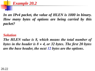
In an IPv4packet, the value of HLEN is 1000 in binary.
How many bytes of options are being carried by this
packet?
Solution
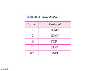
The HLEN value is 8, which means the total number of
bytes in the header is 8 × 4, or 32 bytes. The first 20 bytes
are the base header, the next 12 bytes are the options.
Example 20.2
82.
20.23
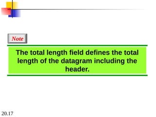
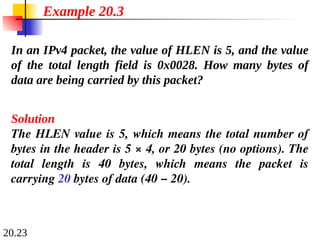
In an IPv4packet, the value of HLEN is 5, and the value
of the total length field is 0x0028. How many bytes of
data are being carried by this packet?
Solution
The HLEN value is 5, which means the total number of
bytes in the header is 5 × 4, or 20 bytes (no options). The
total length is 40 bytes, which means the packet is
carrying 20 bytes of data (40 − 20).
Example 20.3
83.
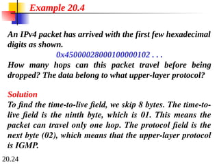
20.24
An IPv4 packethas arrived with the first few hexadecimal
digits as shown.
0x45000028000100000102 . . .
How many hops can this packet travel before being
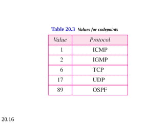
dropped? The data belong to what upper-layer protocol?
Solution
To find the time-to-live field, we skip 8 bytes. The time-to-
live field is the ninth byte, which is 01. This means the
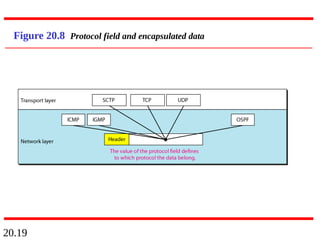
packet can travel only one hop. The protocol field is the
next byte (02), which means that the upper-layer protocol
is IGMP.
Example 20.4
20.30
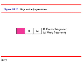
A packet hasarrived with an M bit value of 0. Is this the
first fragment, the last fragment, or a middle fragment?
Do we know if the packet was fragmented?
Solution
If the M bit is 0, it means that there are no more
fragments; the fragment is the last one. However, we
cannot say if the original packet was fragmented or not. A
non-fragmented packet is considered the last fragment.
Example 20.5
90.
20.31
A packet hasarrived with an M bit value of 1. Is this the
first fragment, the last fragment, or a middle fragment?
Do we know if the packet was fragmented?
Solution
If the M bit is 1, it means that there is at least one more
fragment. This fragment can be the first one or a middle
one, but not the last one. We don’t know if it is the first
one or a middle one; we need more information (the value
of the fragmentation offset).
Example 20.6
91.
20.32
A packet hasarrived with an M bit value of 1 and a
fragmentation offset value of 0. Is this the first fragment,
the last fragment, or a middle fragment?
Solution
Because the M bit is 1, it is either the first fragment or a
middle one. Because the offset value is 0, it is the first
fragment.
Example 20.7
92.
20.33
A packet hasarrived in which the offset value is 100.
What is the number of the first byte? Do we know the
number of the last byte?
Solution
To find the number of the first byte, we multiply the offset
value by 8. This means that the first byte number is 800.
We cannot determine the number of the last byte unless
we know the length.
Example 20.8
93.
20.34
A packet hasarrived in which the offset value is 100, the
value of HLEN is 5, and the value of the total length field
is 100. What are the numbers of the first byte and the last
byte?
Solution
The first byte number is 100 × 8 = 800. The total length is
100 bytes, and the header length is 20 bytes (5 × 4), which
means that there are 80 bytes in this datagram. If the first
byte number is 800, the last byte number must be 879.
Example 20.9
94.
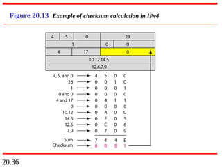
20.35
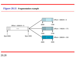
Figure 20.13 showsan example of a checksum
calculation for an IPv4 header without options. The
header is divided into 16-bit sections. All the sections are
added and the sum is complemented. The result is
inserted in the checksum field.
Example 20.10
20.38
20-3 IPv6
20-3 IPv6
Thenetwork layer protocol in the TCP/IP protocol
The network layer protocol in the TCP/IP protocol
suite is currently IPv4. Although IPv4 is well designed,
suite is currently IPv4. Although IPv4 is well designed,
data communication has evolved since the inception of
data communication has evolved since the inception of
IPv4 in the 1970s. IPv4 has some deficiencies that
IPv4 in the 1970s. IPv4 has some deficiencies that
make it unsuitable for the fast-growing Internet.
make it unsuitable for the fast-growing Internet.
Advantages
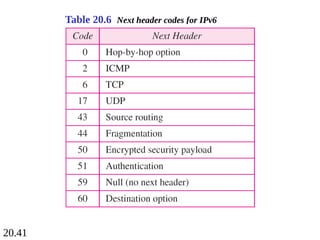
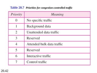
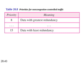
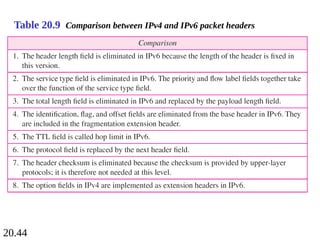
Packet Format
Extension Headers
Topics discussed in this section:
Topics discussed in this section:
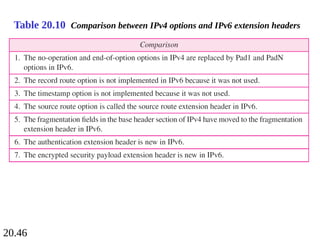
20.47
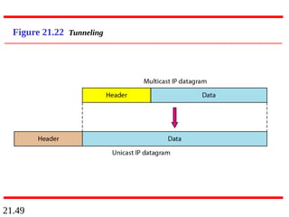
20-4 TRANSITION FROMIPv4 TO IPv6
20-4 TRANSITION FROM IPv4 TO IPv6
Because of the huge number of systems on the
Because of the huge number of systems on the
Internet, the transition from IPv4 to IPv6 cannot
Internet, the transition from IPv4 to IPv6 cannot
happen suddenly. It takes a considerable amount of
happen suddenly. It takes a considerable amount of
time before every system in the Internet can move from
time before every system in the Internet can move from
IPv4 to IPv6. The transition must be smooth to prevent
IPv4 to IPv6. The transition must be smooth to prevent
any problems between IPv4 and IPv6 systems.
any problems between IPv4 and IPv6 systems.
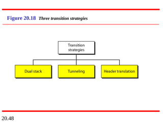
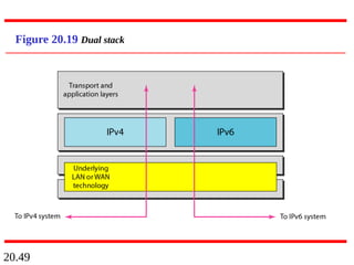
Dual Stack
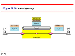
Tunneling
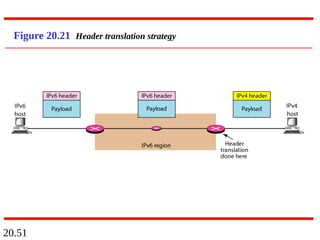
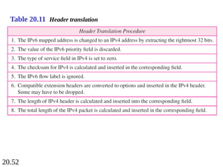
Header Translation
Topics discussed in this section:
Topics discussed in this section:
21.2
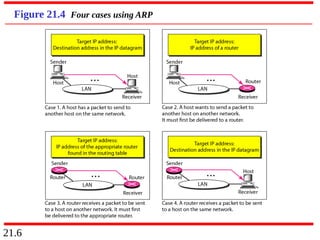
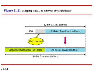
21-1 ADDRESS MAPPING
21-1ADDRESS MAPPING
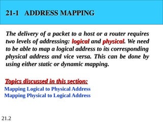
The delivery of a packet to a host or a router requires
The delivery of a packet to a host or a router requires
two levels of addressing:
two levels of addressing: logical
logical and
and physical
physical. We need
. We need
to be able to map a logical address to its corresponding
to be able to map a logical address to its corresponding
physical address and vice versa. This can be done by
physical address and vice versa. This can be done by
using either static or dynamic mapping.
using either static or dynamic mapping.
Mapping Logical to Physical Address
Mapping Physical to Logical Address
Topics discussed in this section:
Topics discussed in this section:
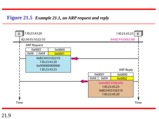
21.8
A host withIP address 130.23.43.20 and physical address
B2:34:55:10:22:10 has a packet to send to another host
with IP address 130.23.43.25 and physical address
A4:6E:F4:59:83:AB. The two hosts are on the same
Ethernet network. Show the ARP request and reply
packets encapsulated in Ethernet frames.
Solution
Figure 21.5 shows the ARP request and reply packets.
Note that the ARP data field in this case is 28 bytes, and
that the individual addresses do not fit in the 4-byte
boundary. That is why we do not show the regular 4-byte
boundaries for these addresses.
Example 21.1
21.13
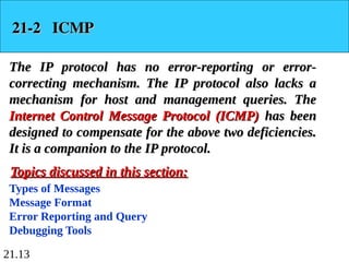
21-2 ICMP
21-2 ICMP
TheIP protocol has no error-reporting or error-
The IP protocol has no error-reporting or error-
correcting mechanism. The IP protocol also lacks a
correcting mechanism. The IP protocol also lacks a
mechanism for host and management queries. The
mechanism for host and management queries. The
Internet Control Message Protocol (ICMP)
Internet Control Message Protocol (ICMP) has been
has been
designed to compensate for the above two deficiencies.
designed to compensate for the above two deficiencies.
It is a companion to the IP protocol.
It is a companion to the IP protocol.
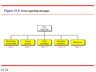
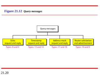
Types of Messages
Message Format
Error Reporting and Query
Debugging Tools
Topics discussed in this section:
Topics discussed in this section:
21.17
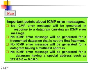
Important points aboutICMP error messages:
❏ No ICMP error message will be generated in
response to a datagram carrying an ICMP error
message.
❏ No ICMP error message will be generated for a
fragmented datagram that is not the first fragment.
❏ No ICMP error message will be generated for a
datagram having a multicast address.
❏ No ICMP error message will be generated for a
datagram having a special address such as
127.0.0.0 or 0.0.0.0.
Note
21.22
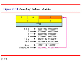
Figure 21.14 showsan example of checksum calculation
for a simple echo-request message. We randomly chose
the identifier to be 1 and the sequence number to be 9.
The message is divided into 16-bit (2-byte) words. The
words are added and the sum is complemented. Now the
sender can put this value in the checksum field.
Example 21.2
21.24
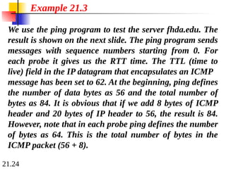
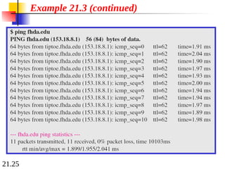
We use theping program to test the server fhda.edu. The
result is shown on the next slide. The ping program sends
messages with sequence numbers starting from 0. For
each probe it gives us the RTT time. The TTL (time to
live) field in the IP datagram that encapsulates an ICMP
message has been set to 62. At the beginning, ping defines
the number of data bytes as 56 and the total number of
bytes as 84. It is obvious that if we add 8 bytes of ICMP
header and 20 bytes of IP header to 56, the result is 84.
However, note that in each probe ping defines the number
of bytes as 64. This is the total number of bytes in the
ICMP packet (56 + 8).
Example 21.3
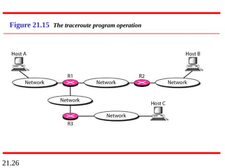
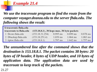
21.27
We use thetraceroute program to find the route from the
computer voyager.deanza.edu to the server fhda.edu. The
following shows the result:
Example 21.4
The unnumbered line after the command shows that the
destination is 153.18.8.1. The packet contains 38 bytes: 20
bytes of IP header, 8 bytes of UDP header, and 10 bytes of
application data. The application data are used by
traceroute to keep track of the packets.
139.
21.28
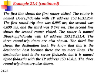
The first lineshows the first router visited. The router is
named Dcore.fhda.edu with IP address 153.18.31.254.
The first round-trip time was 0.995 ms, the second was
0.899 ms, and the third was 0.878 ms. The second line
shows the second router visited. The router is named
Dbackup.fhda.edu with IP address 153.18.251.4. The
three round-trip times are also shown. The third line
shows the destination host. We know that this is the
destination host because there are no more lines. The
destination host is the server fhda.edu, but it is named
tiptoe.fhda.edu with the IP address 153.18.8.1. The three
round-trip times are also shown.
Example 21.4 (continued)
140.
21.29
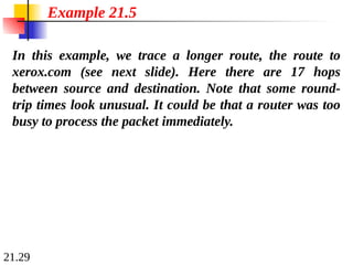
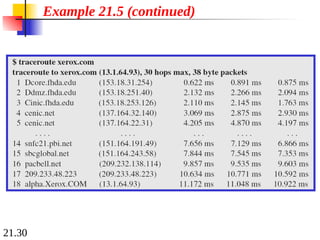
In this example,we trace a longer route, the route to
xerox.com (see next slide). Here there are 17 hops
between source and destination. Note that some round-
trip times look unusual. It could be that a router was too
busy to process the packet immediately.
Example 21.5
21.31
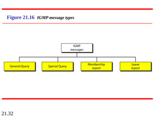
21-3 IGMP
21-3 IGMP
TheIP protocol can be involved in two types of
The IP protocol can be involved in two types of
communication: unicasting and multicasting. The
communication: unicasting and multicasting. The
Internet Group Management Protocol (IGMP) is one
Internet Group Management Protocol (IGMP) is one
of the necessary, but not sufficient, protocols that is
of the necessary, but not sufficient, protocols that is
involved in multicasting. IGMP is a companion to the
involved in multicasting. IGMP is a companion to the
IP protocol.
IP protocol.
Group Management
IGMP Messages and IGMP Operation
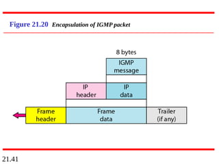
Encapsulation
Netstat Utility
Topics discussed in this section:
Topics discussed in this section:
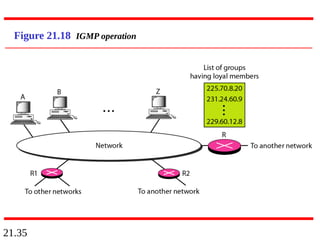
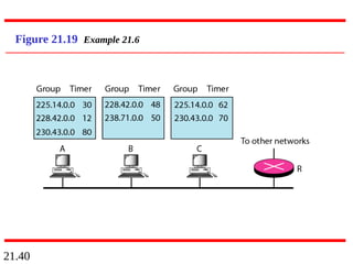
21.38
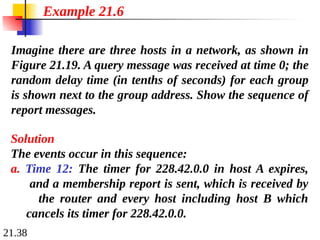
Imagine there arethree hosts in a network, as shown in
Figure 21.19. A query message was received at time 0; the
random delay time (in tenths of seconds) for each group
is shown next to the group address. Show the sequence of
report messages.
Example 21.6
Solution
The events occur in this sequence:
a. Time 12: The timer for 228.42.0.0 in host A expires,
and a membership report is sent, which is received by
the router and every host including host B which
cancels its timer for 228.42.0.0.
150.
21.39
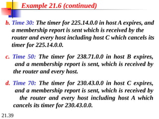
Example 21.6 (continued)
b.Time 30: The timer for 225.14.0.0 in host A expires, and
a membership report is sent which is received by the
router and every host including host C which cancels its
timer for 225.14.0.0.
c. Time 50: The timer for 238.71.0.0 in host B expires,
and a membership report is sent, which is received by
the router and every host.
d. Time 70: The timer for 230.43.0.0 in host C expires,
and a membership report is sent, which is received by
the router and every host including host A which
cancels its timer for 230.43.0.0.
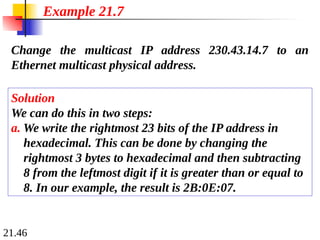
21.46
Change the multicastIP address 230.43.14.7 to an
Ethernet multicast physical address.
Solution
We can do this in two steps:
a. We write the rightmost 23 bits of the IP address in
hexadecimal. This can be done by changing the
rightmost 3 bytes to hexadecimal and then subtracting
8 from the leftmost digit if it is greater than or equal to
8. In our example, the result is 2B:0E:07.
Example 21.7
158.
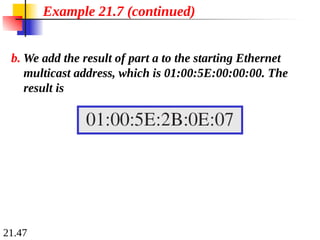
21.47
b. We addthe result of part a to the starting Ethernet
multicast address, which is 01:00:5E:00:00:00. The
result is
Example 21.7 (continued)
159.
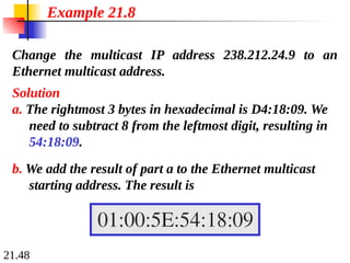
21.48
Change the multicastIP address 238.212.24.9 to an
Ethernet multicast address.
Solution
a. The rightmost 3 bytes in hexadecimal is D4:18:09. We
need to subtract 8 from the leftmost digit, resulting in
54:18:09.
Example 21.8
b. We add the result of part a to the Ethernet multicast
starting address. The result is
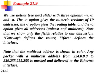
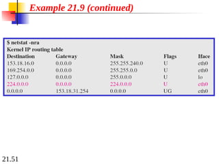
21.50
We use netstat(see next slide) with three options: -n, -r,
and -a. The -n option gives the numeric versions of IP
addresses, the -r option gives the routing table, and the -a
option gives all addresses (unicast and multicast). Note
that we show only the fields relative to our discussion.
“Gateway” defines the router, “Iface” defines the
interface.
Note that the multicast address is shown in color. Any
packet with a multicast address from 224.0.0.0 to
239.255.255.255 is masked and delivered to the Ethernet
interface.
Example 21.9
21.52
21-4 ICMPv6
21-4 ICMPv6
Wediscussed IPv6 in Chapter 20. Another protocol
We discussed IPv6 in Chapter 20. Another protocol
that has been modified in version 6 of the TCP/IP
that has been modified in version 6 of the TCP/IP
protocol suite is ICMP (ICMPv6). This new version
protocol suite is ICMP (ICMPv6). This new version
follows the same strategy and purposes of version 4.
follows the same strategy and purposes of version 4.
Error Reporting
Query
Topics discussed in this section:
Topics discussed in this section:
22.2
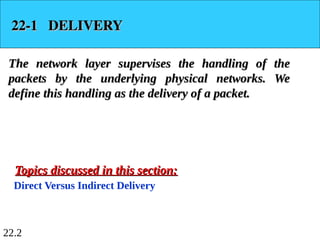
22-1 DELIVERY
22-1 DELIVERY
Thenetwork layer supervises the handling of the
The network layer supervises the handling of the
packets by the underlying physical networks. We
packets by the underlying physical networks. We
define this handling as the delivery of a packet.
define this handling as the delivery of a packet.
Direct Versus Indirect Delivery
Topics discussed in this section:
Topics discussed in this section:
22.4
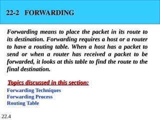
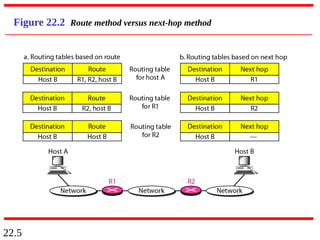
22-2 FORWARDING
22-2 FORWARDING
Forwardingmeans to place the packet in its route to
Forwarding means to place the packet in its route to
its destination. Forwarding requires a host or a router
its destination. Forwarding requires a host or a router
to have a routing table. When a host has a packet to
to have a routing table. When a host has a packet to
send or when a router has received a packet to be
send or when a router has received a packet to be
forwarded, it looks at this table to find the route to the
forwarded, it looks at this table to find the route to the
final destination.
final destination.
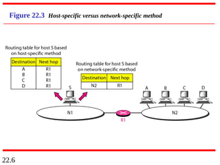
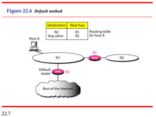
Forwarding Techniques
Forwarding Process
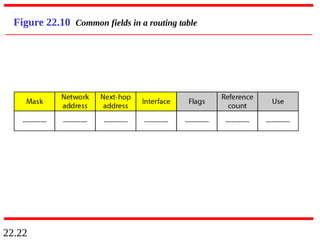
Routing Table
Topics discussed in this section:
Topics discussed in this section:
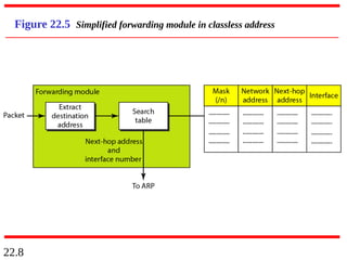
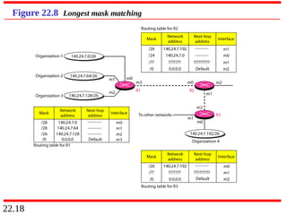
22.13
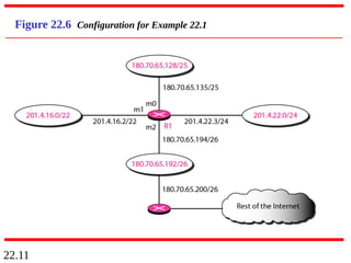
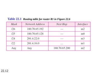
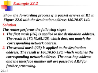
Show the forwardingprocess if a packet arrives at R1 in
Figure 22.6 with the destination address 180.70.65.140.
Example 22.2
Solution
The router performs the following steps:
1. The first mask (/26) is applied to the destination address.
The result is 180.70.65.128, which does not match the
corresponding network address.
2. The second mask (/25) is applied to the destination
address. The result is 180.70.65.128, which matches the
corresponding network address. The next-hop address
and the interface number m0 are passed to ARP for
further processing.
180.
22.14
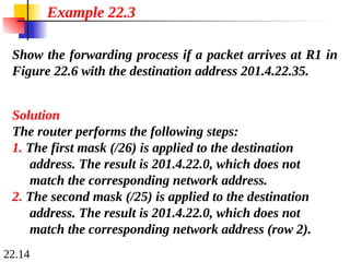
Show the forwardingprocess if a packet arrives at R1 in
Figure 22.6 with the destination address 201.4.22.35.
Example 22.3
Solution
The router performs the following steps:
1. The first mask (/26) is applied to the destination
address. The result is 201.4.22.0, which does not
match the corresponding network address.
2. The second mask (/25) is applied to the destination
address. The result is 201.4.22.0, which does not
match the corresponding network address (row 2).
181.
22.15
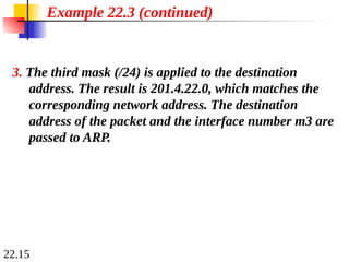
Example 22.3 (continued)
3.The third mask (/24) is applied to the destination
address. The result is 201.4.22.0, which matches the
corresponding network address. The destination
address of the packet and the interface number m3 are
passed to ARP.
182.
22.16
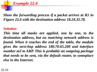
Show the forwardingprocess if a packet arrives at R1 in
Figure 22.6 with the destination address 18.24.32.78.
Example 22.4
Solution
This time all masks are applied, one by one, to the
destination address, but no matching network address is
found. When it reaches the end of the table, the module
gives the next-hop address 180.70.65.200 and interface
number m2 to ARP. This is probably an outgoing package
that needs to be sent, via the default router, to someplace
else in the Internet.
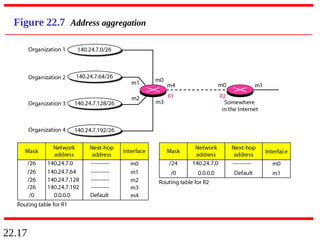
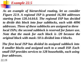
22.19
As an exampleof hierarchical routing, let us consider
Figure 22.9. A regional ISP is granted 16,384 addresses
starting from 120.14.64.0. The regional ISP has decided
to divide this block into four subblocks, each with 4096
addresses. Three of these subblocks are assigned to three
local ISPs; the second subblock is reserved for future use.
Note that the mask for each block is /20 because the
original block with mask /18 is divided into 4 blocks.
Example 22.5
The first local ISP has divided its assigned subblock into
8 smaller blocks and assigned each to a small ISP. Each
small ISP provides services to 128 households, each using
four addresses.
186.
22.20
The second localISP has divided its block into 4 blocks
and has assigned the addresses to four large
organizations.
Example 22.5 (continued)
There is a sense of hierarchy in this configuration. All
routers in the Internet send a packet with destination
address 120.14.64.0 to 120.14.127.255 to the regional ISP.
The third local ISP has divided its block into 16 blocks
and assigned each block to a small organization. Each
small organization has 256 addresses, and the mask is /
24.
22.23
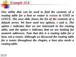
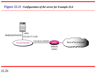
One utility thatcan be used to find the contents of a
routing table for a host or router is netstat in UNIX or
LINUX. The next slide shows the list of the contents of a
default server. We have used two options, r and n. The
option r indicates that we are interested in the routing
table, and the option n indicates that we are looking for
numeric addresses. Note that this is a routing table for a
host, not a router. Although we discussed the routing table
for a router throughout the chapter, a host also needs a
routing table.
Example 22.6
190.
22.24
Example 22.6 (continued)
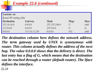
Thedestination column here defines the network address.
The term gateway used by UNIX is synonymous with
router. This column actually defines the address of the next
hop. The value 0.0.0.0 shows that the delivery is direct. The
last entry has a flag of G, which means that the destination
can be reached through a router (default router). The Iface
defines the interface.
191.
22.25
Example 22.6 (continued)
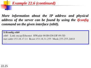
Moreinformation about the IP address and physical
address of the server can be found by using the ifconfig
command on the given interface (eth0).
22.27
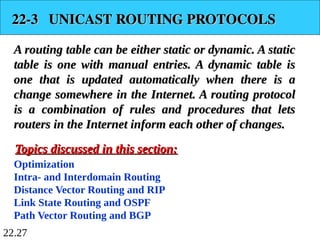
22-3 UNICAST ROUTINGPROTOCOLS
22-3 UNICAST ROUTING PROTOCOLS
A routing table can be either static or dynamic. A static
A routing table can be either static or dynamic. A static
table is one with manual entries. A dynamic table is
table is one with manual entries. A dynamic table is
one that is updated automatically when there is a
one that is updated automatically when there is a
change somewhere in the Internet. A routing protocol
change somewhere in the Internet. A routing protocol
is a combination of rules and procedures that lets
is a combination of rules and procedures that lets
routers in the Internet inform each other of changes.
routers in the Internet inform each other of changes.
Optimization
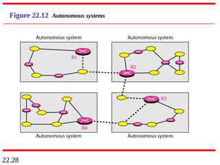
Intra- and Interdomain Routing
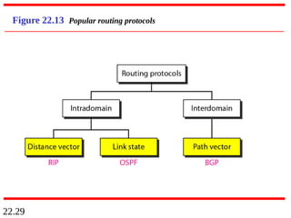
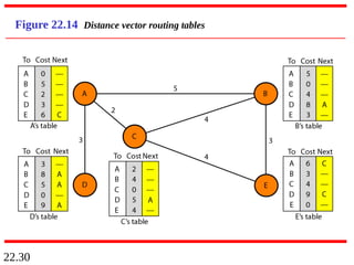
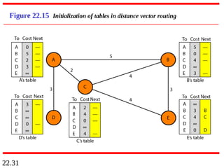
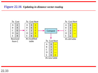
Distance Vector Routing and RIP
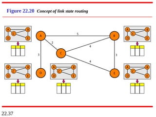
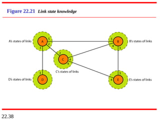
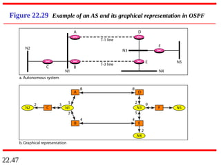
Link State Routing and OSPF
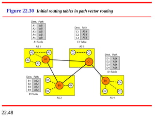
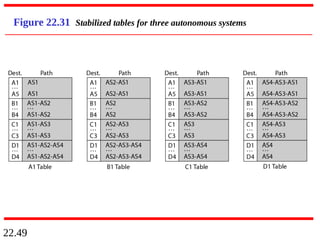
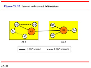
Path Vector Routing and BGP
Topics discussed in this section:
Topics discussed in this section:
22.51
22-4 MULTICAST ROUTINGPROTOCOLS
22-4 MULTICAST ROUTING PROTOCOLS
In this section, we discuss multicasting and multicast
In this section, we discuss multicasting and multicast
routing protocols.
routing protocols.
Unicast, Multicast, and Broadcast
Applications
Multicast Routing
Routing Protocols
Topics discussed in this section:
Topics discussed in this section:
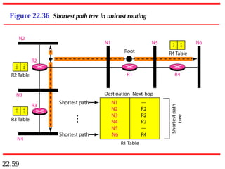
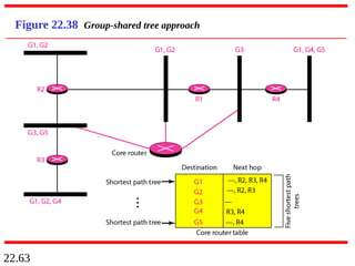
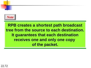
22.72
RPB creates ashortest path broadcast
tree from the source to each destination.
It guarantees that each destination
receives one and only one copy
of the packet.
Note
22.77
In CBT, thesource sends the multicast
packet (encapsulated in a unicast
packet) to the core router. The core
router decapsulates the packet and
forwards it to all interested interfaces.
Note