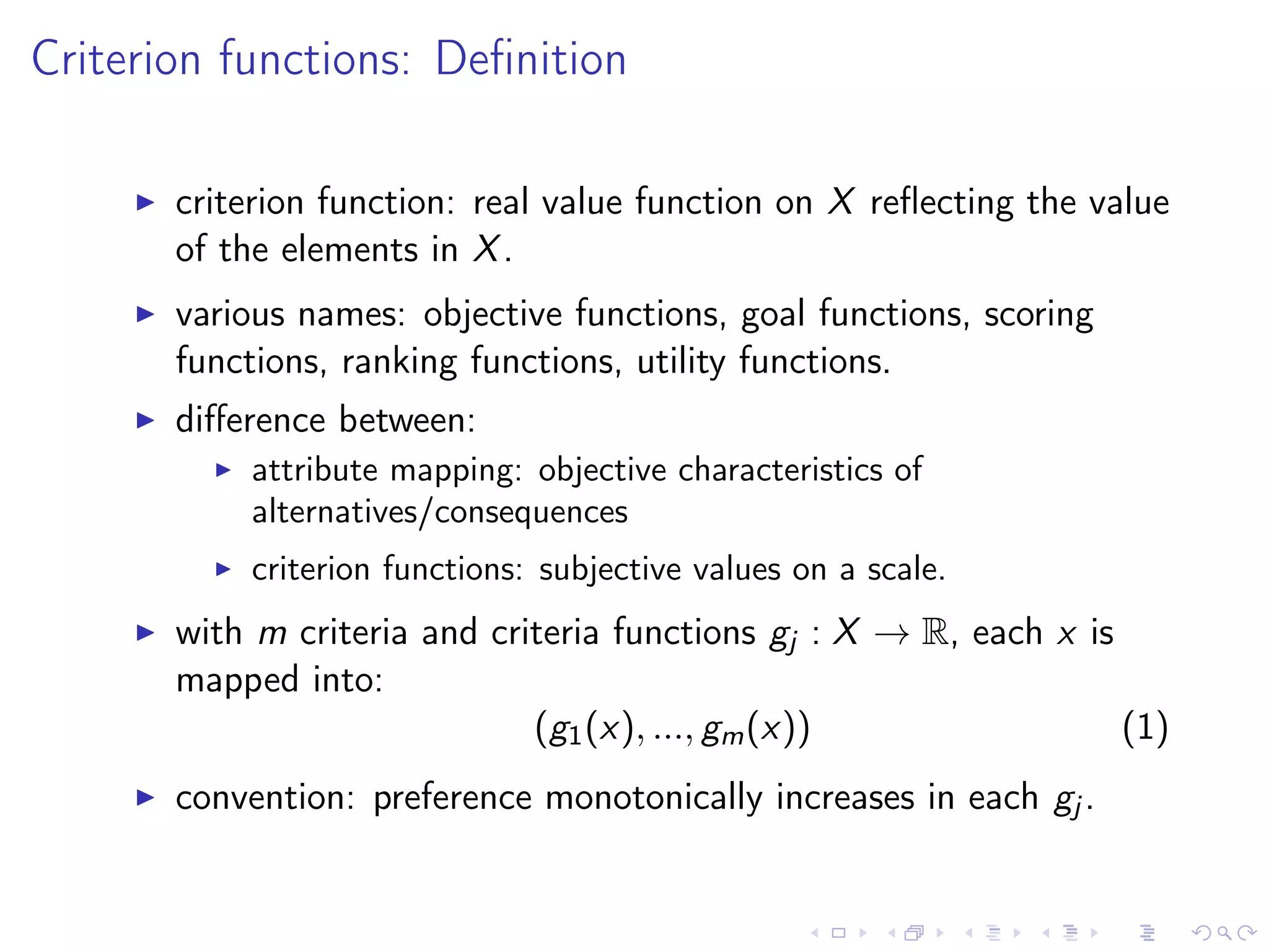
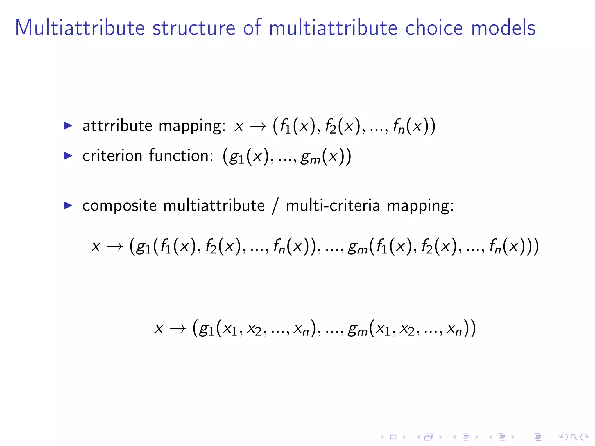
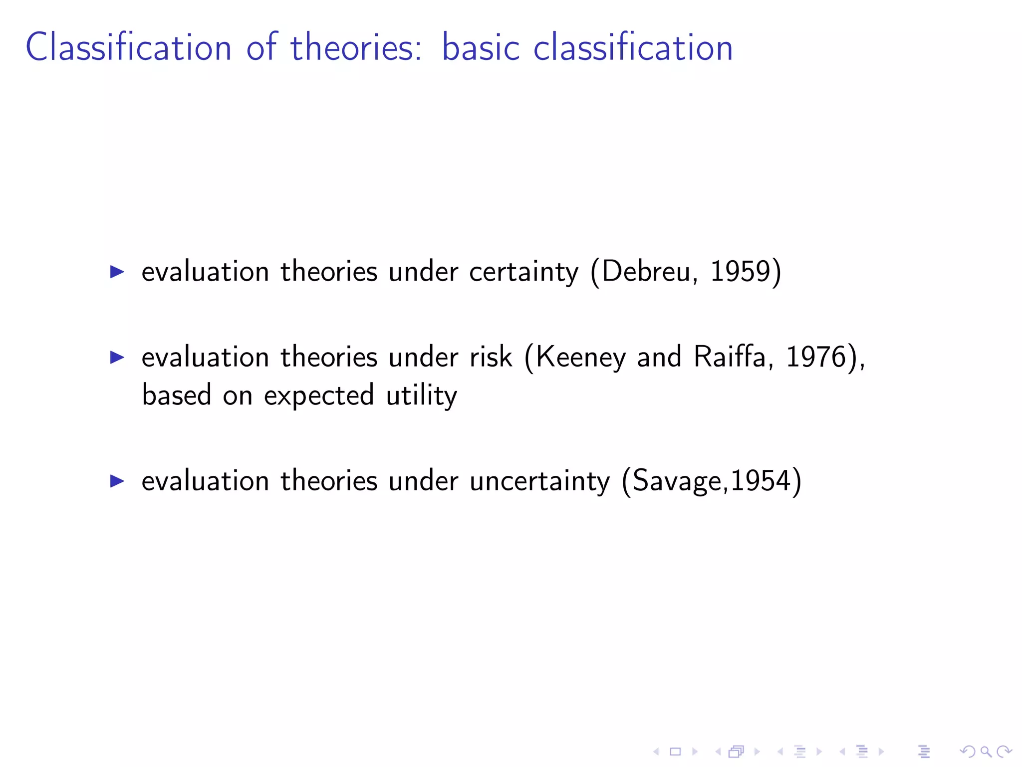
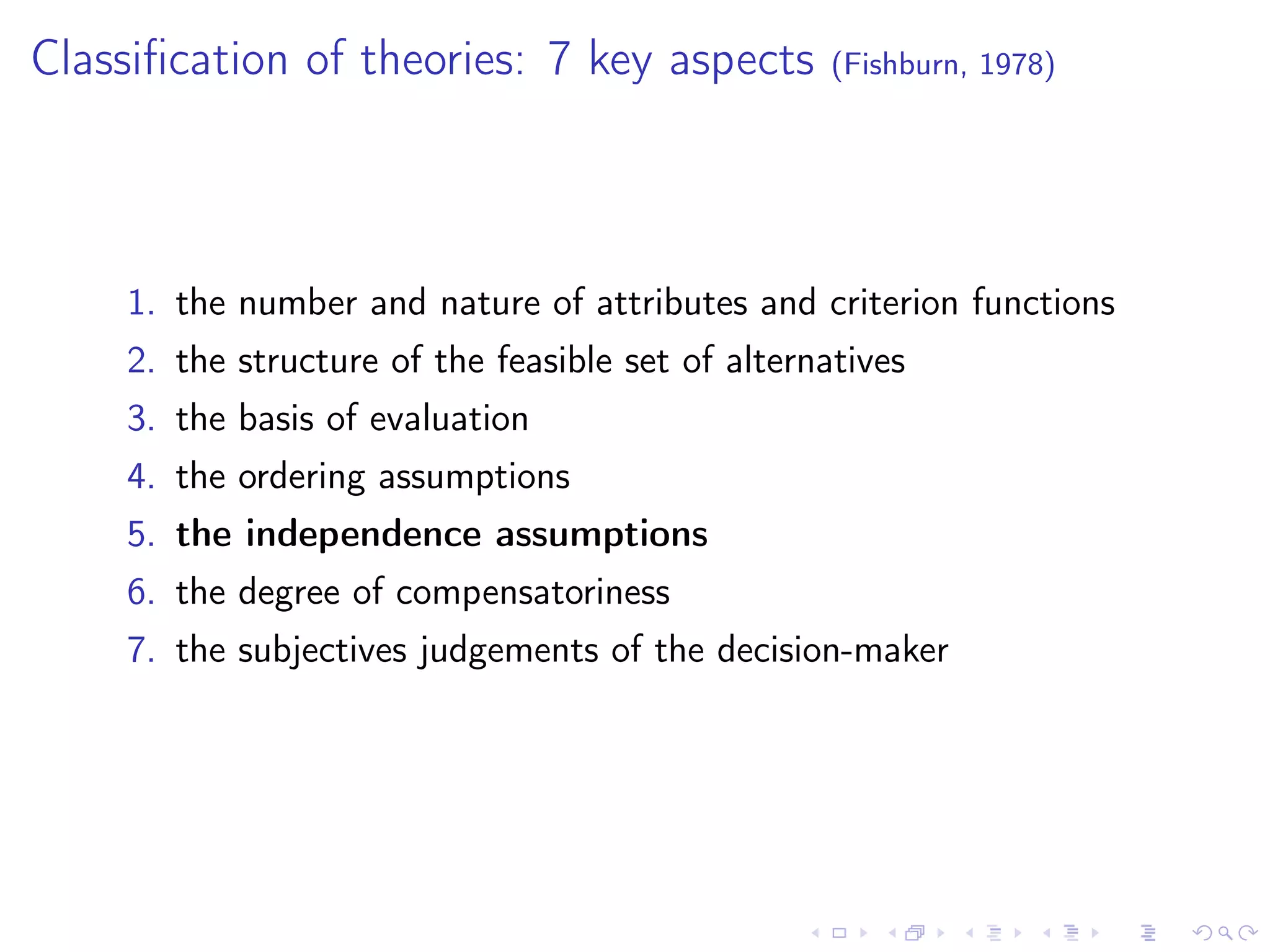
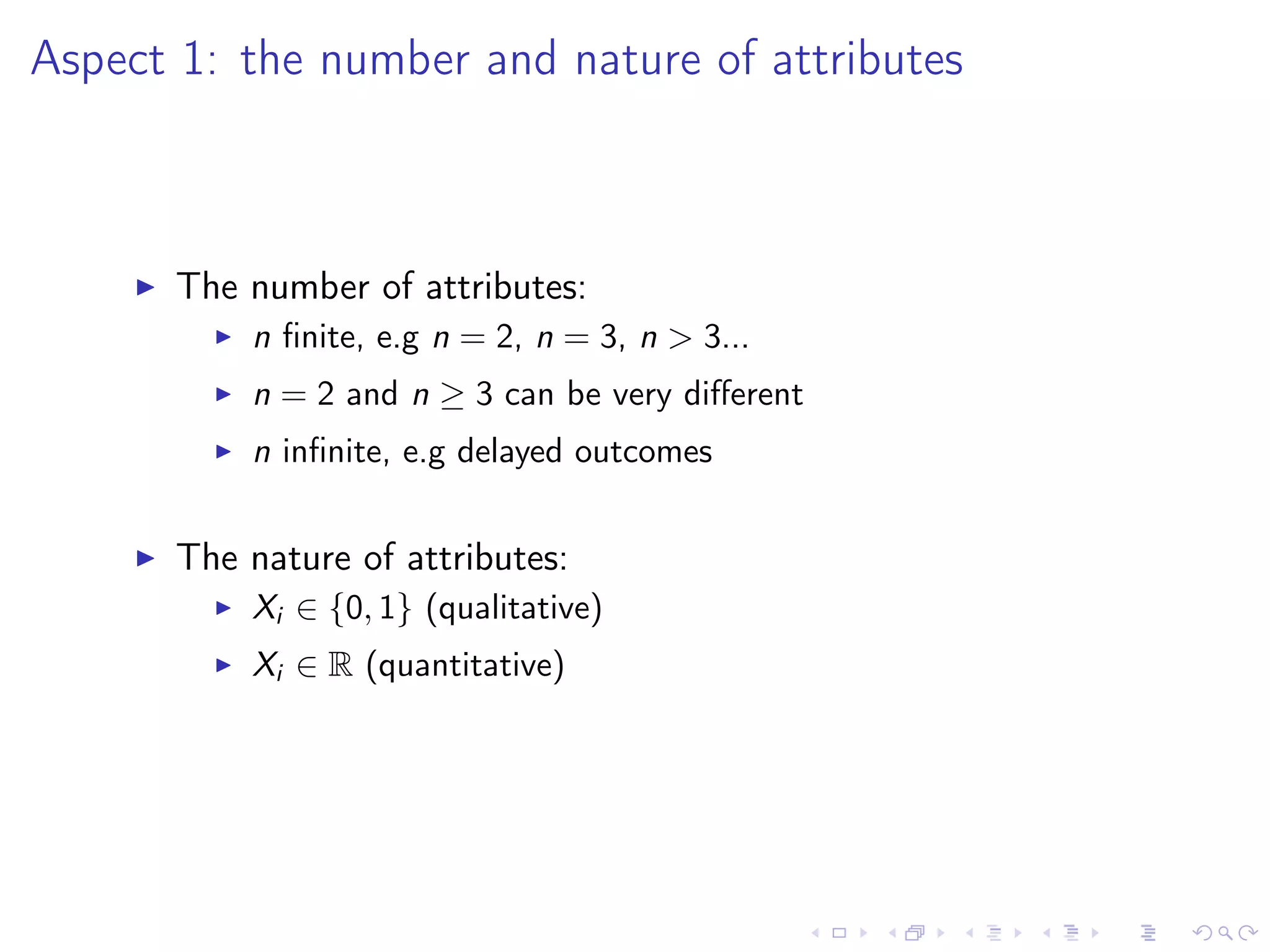
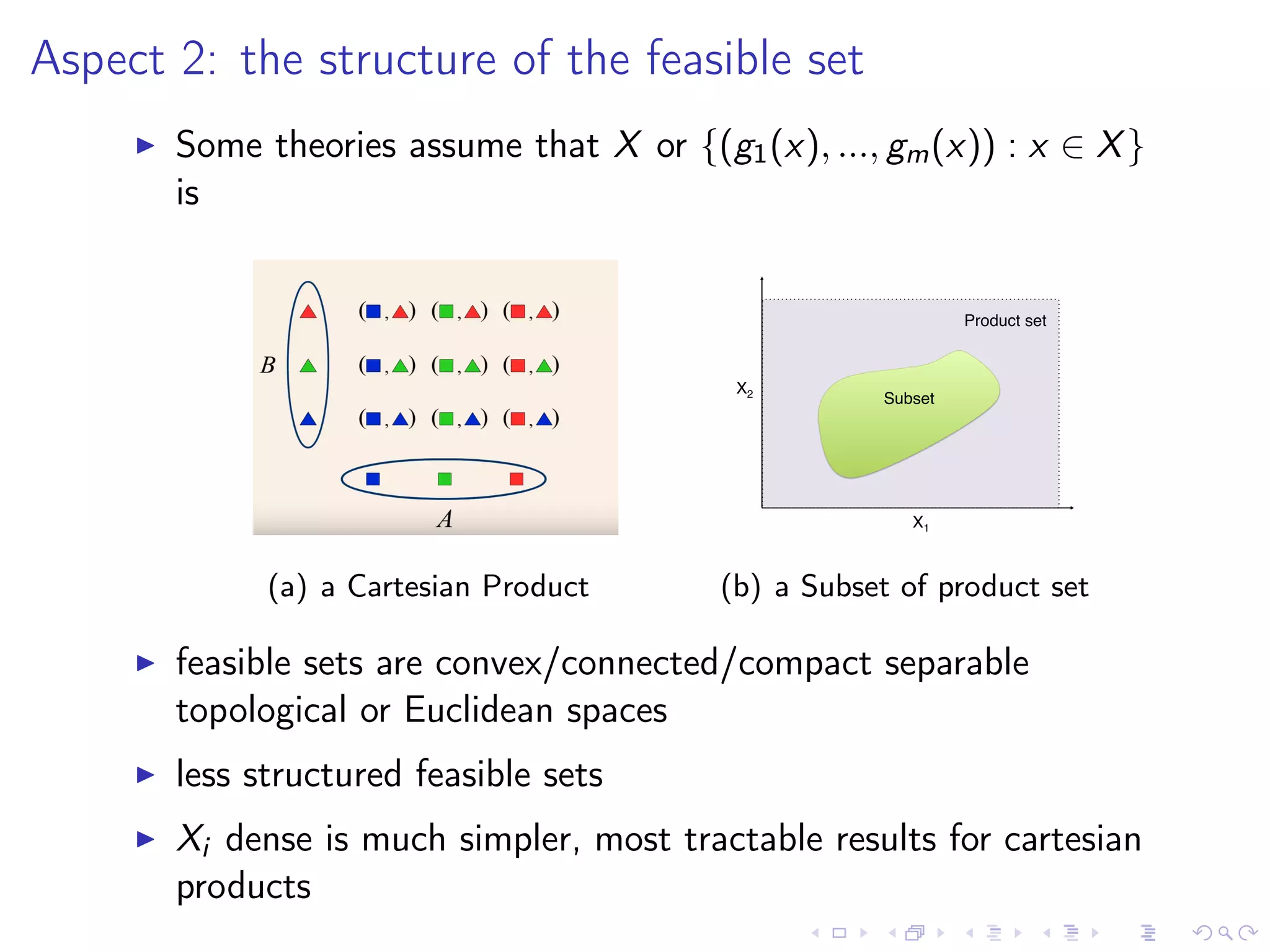
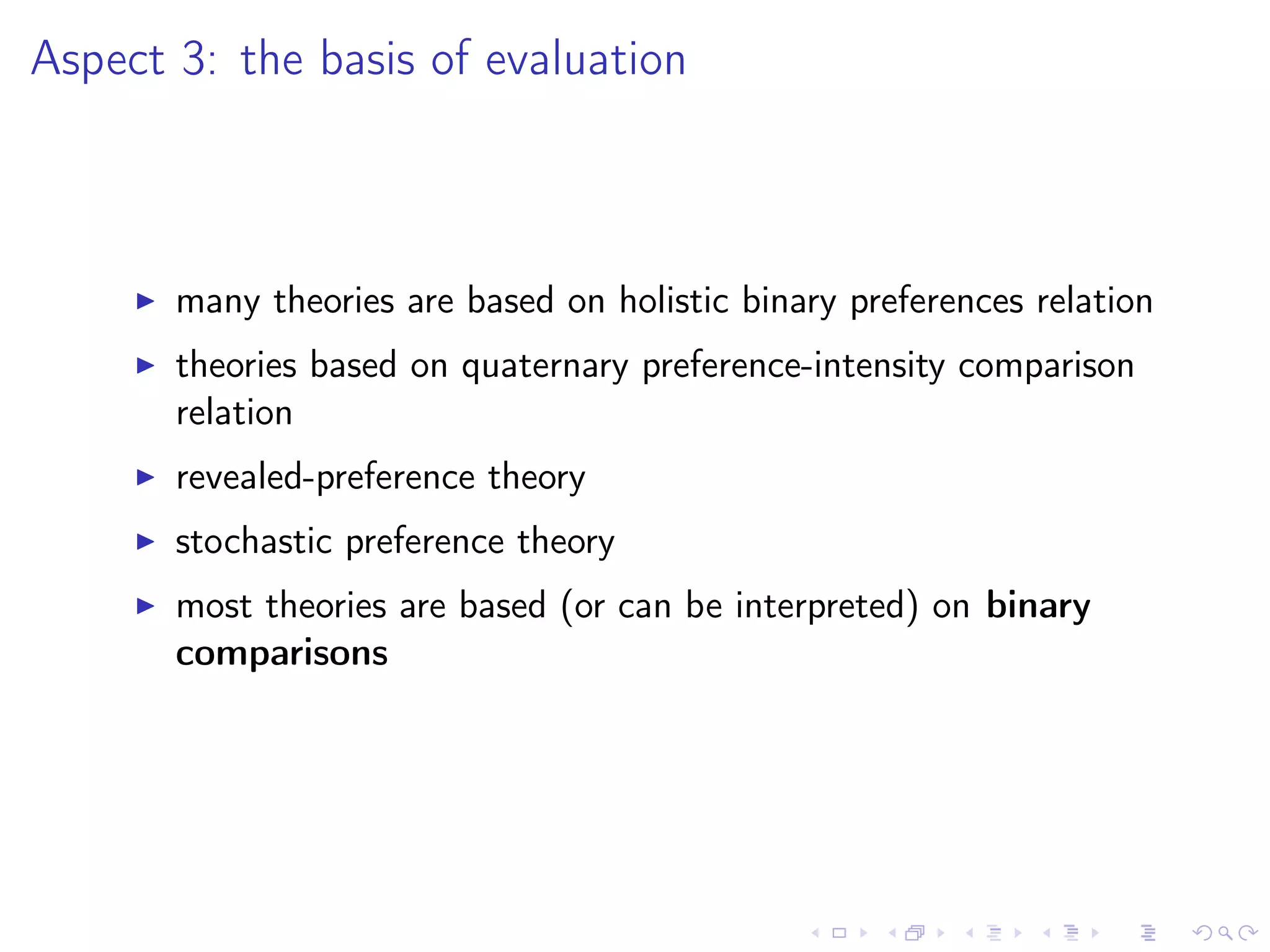
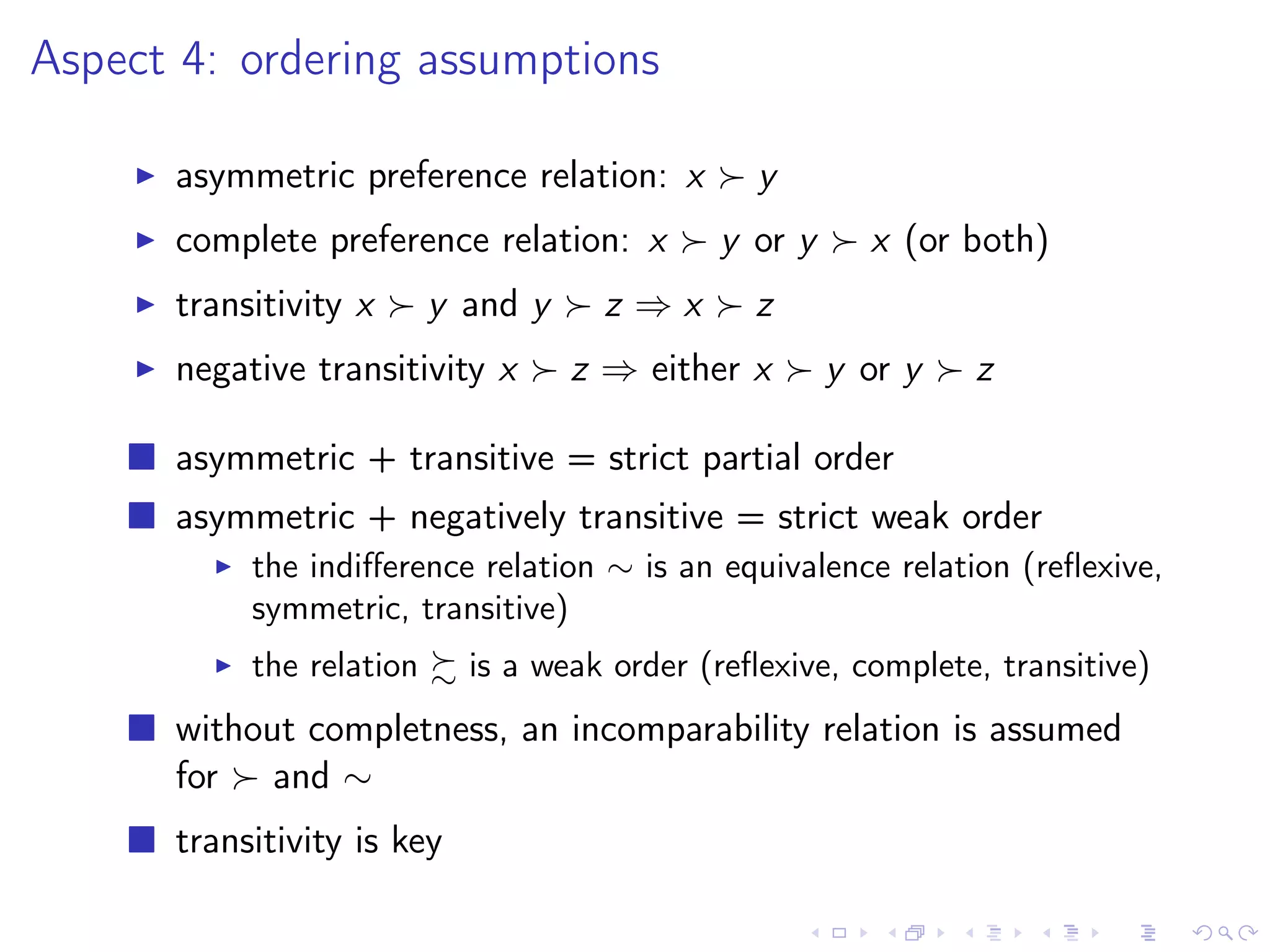
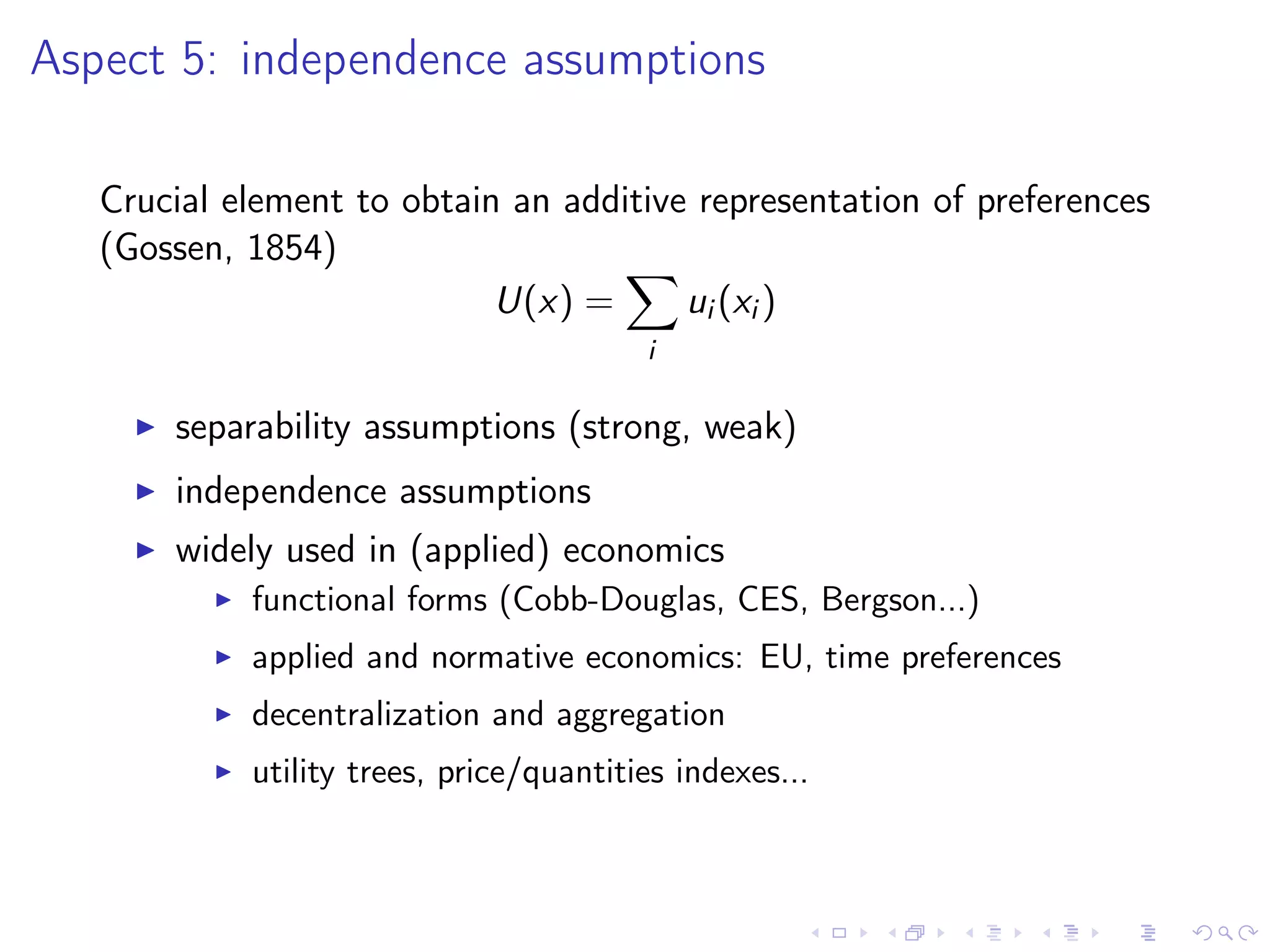
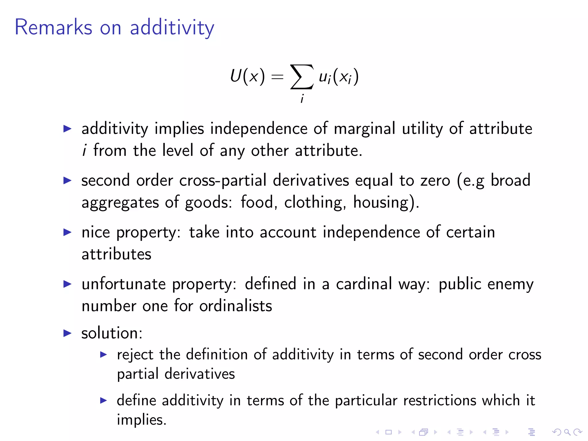
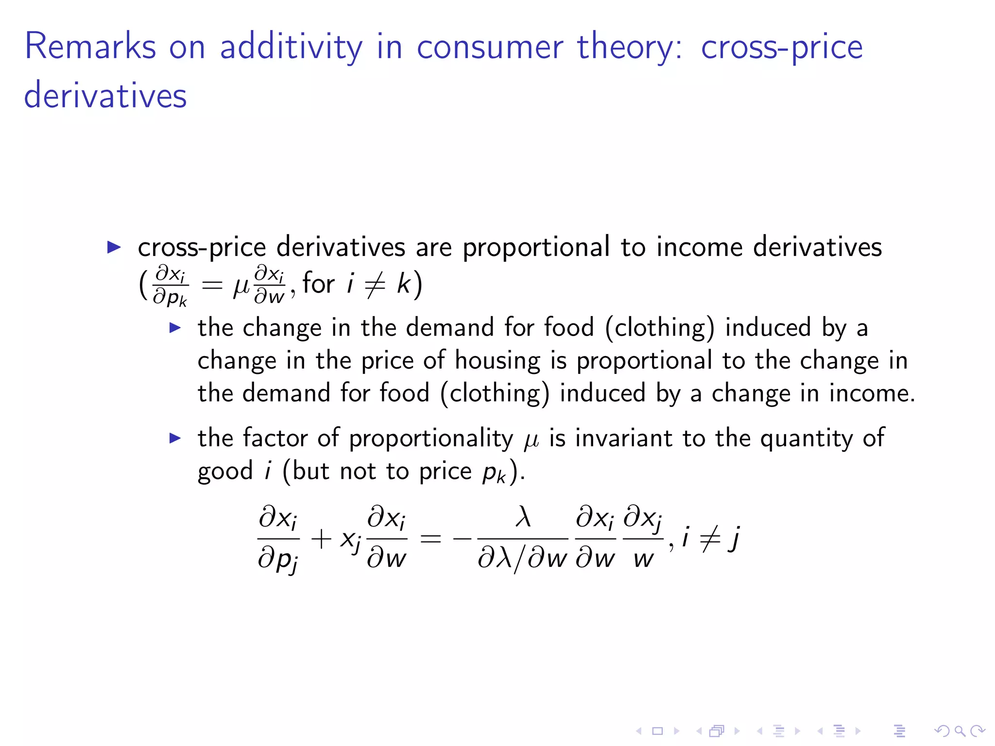
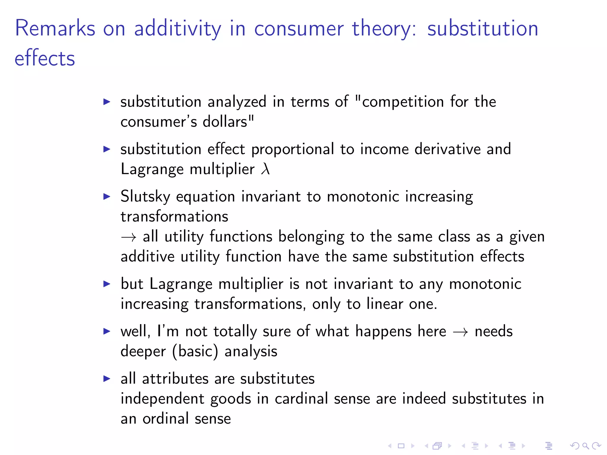
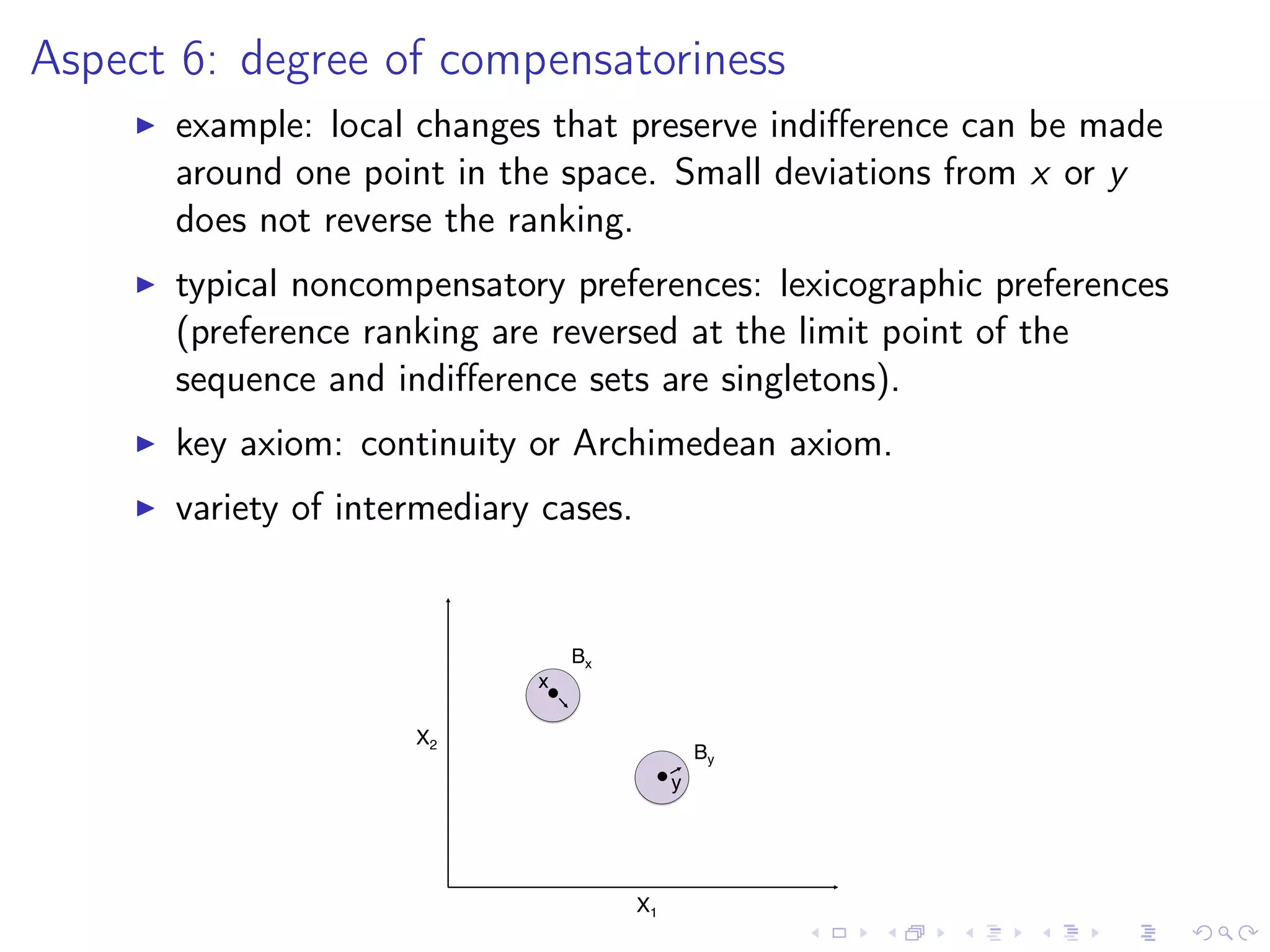
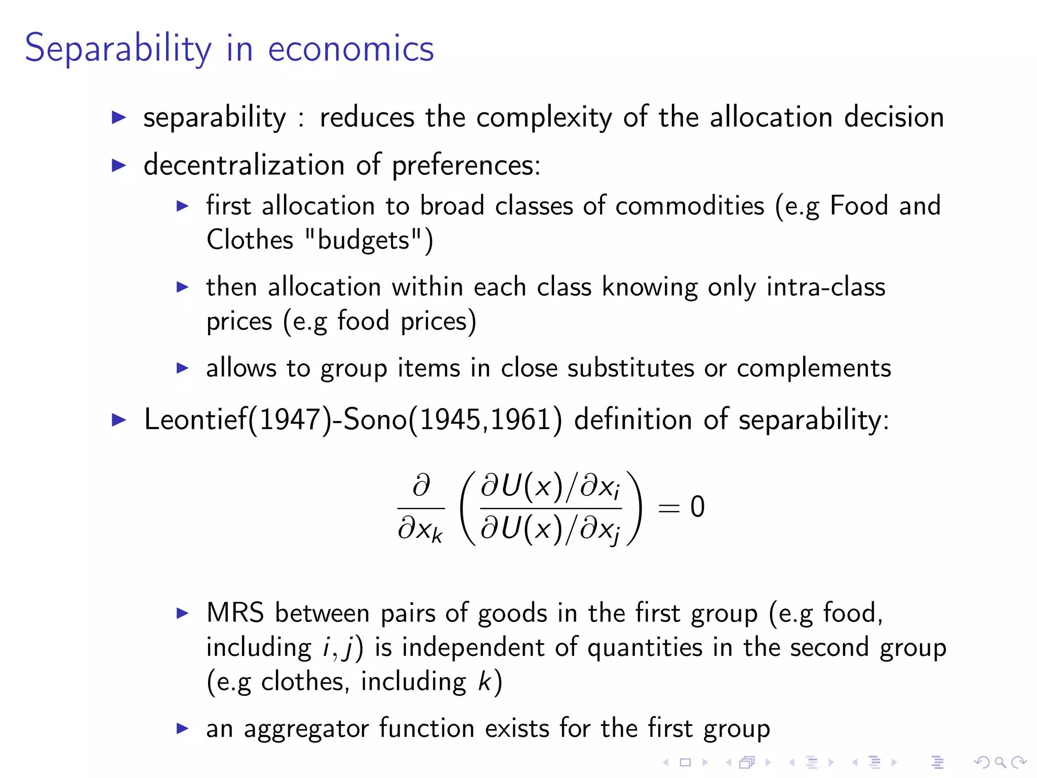
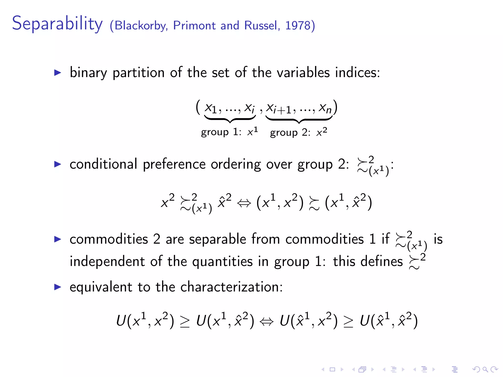
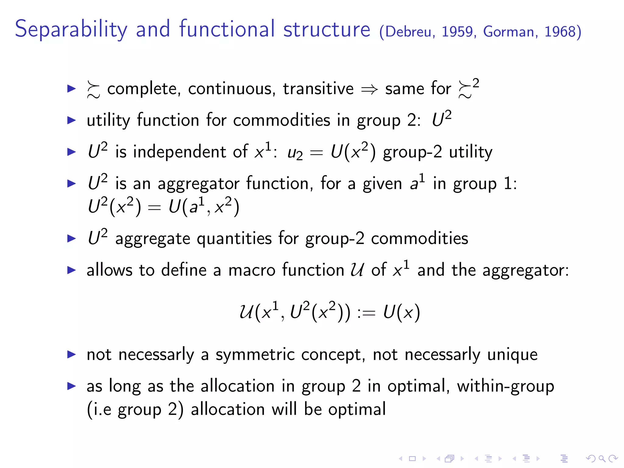
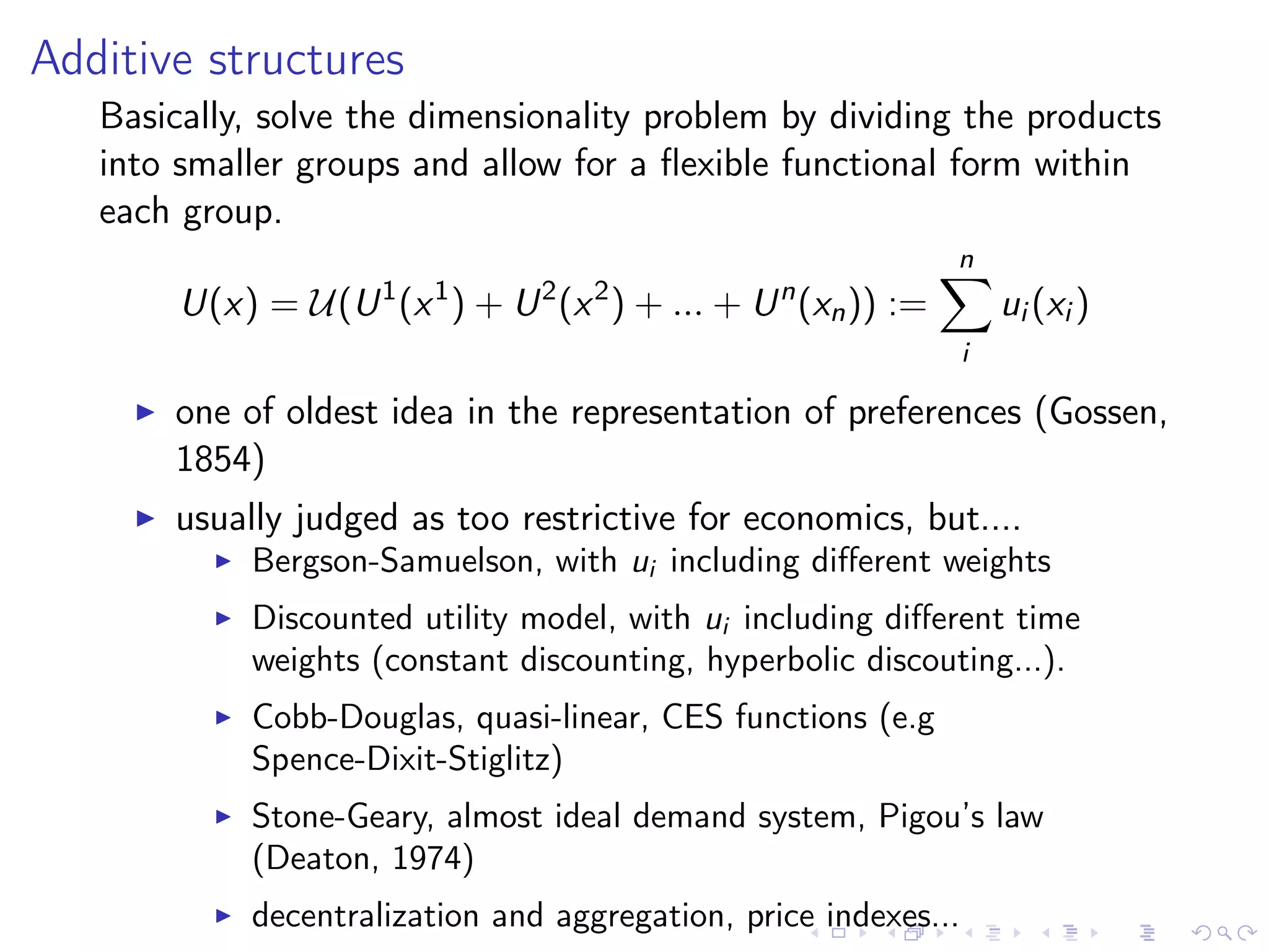
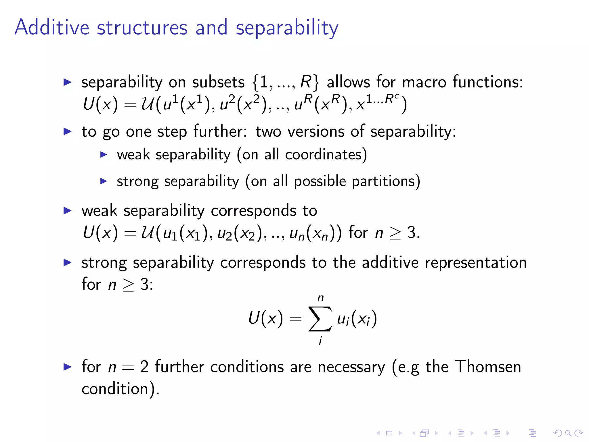
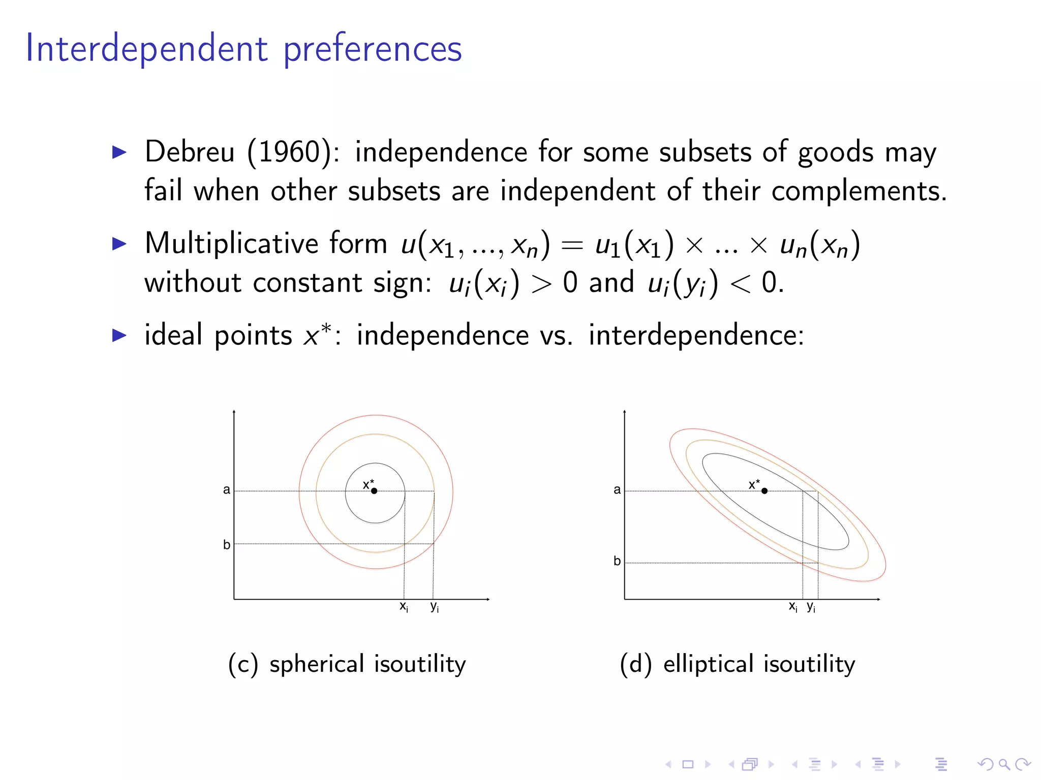
This document provides an introduction to multiattribute decision making and decision theories. It discusses several key aspects of multiattribute choice models, including: 1) The number and nature of attributes that are used to differentiate decision alternatives. 2) The structure of the feasible set of alternatives. 3) The basis of evaluation, such as preference relations or criterion functions. 4) Independence and separability assumptions that are required to obtain additive representations of preferences. The document outlines some classic evaluation theories under certainty that do not involve probabilities, and discusses the concept of separability, which reduces complexity by allowing decentralized preferences across attribute groups.

1. Multiattribute decision making
Part 1: Classics (Fishburn/Kreps/Wakker)
Separability and Independence
Olivier L’Haridon
January 14, 2016

2. Introduction

3. Attribute mapping: Settings
X the set of decision alternatives
n ≥ 2 attributes used to differentiate among the objects in X
∀i ∈ 1...n, there is a set Xi whose elements are values/level of
attribute i
∀i ∈ 1...n, there is an attribute mapping fi : X → Xi
each fi assigns to each object in X a specific level of the ith
attribute.
for each x ∈ X, the fi functions produce a n-tuple
(f1(x), f2(x), ..., fn(x)) in X1 × ... × Xn.

4. Attribute mapping: Settings
The fi functions describes x in terms of its values on the n
attributes.
The fi functions are descriptive or identification functions.
x!
X!
f1!
x1!
X1!
fn!
xn!
Xn!
f2!
x2!
X2!
. . .!
x → (f1(x), f2(x), ..., fn(x))

5. Attribute mapping: Examples
f1(x), f2(x), ..., fn(x)
X is a set of simple probability measures on R and fi (x) is the
ith central moment of x.
X is the set of commodity bundles. In standard
microeconomics fi are linear functions.
X is the set of commodity bundles. In Lancaster (1966)
decision needs to map first each x ∈ X into a vector of
characteristics (f1(x), f2(x), ..., fn(x)).
X is the set of people. In literature on inequality, decision is
often based on a vector of wealths (f1(x), f2(x), ..., fn(x)).

6. Attribute mapping: Remarks
x → (x1, x2, ..., xn)
In many cases, fi (x) is abbreviated as xi and elements in X are
n-tuples (x1, ..., xn) in the product set X1 × ... × Xn.
X is a proper subset of X1 × .... × Xn: X ⊆ X1 × .... × Xn.
elements of X1 × .... × Xn that are not in X are unrealizable or
infeasable combinations of attributes.
many axiomatic preference theories assume that
X = X1 × .... × Xn.
implicit assumption of attribute mapping (non neutral): two
elements in X that map in the same n-tuple (x1, ..., xn) are
indifferent/ have equal value.

7. Criterion functions: Definition
criterion function: real value function on X reflecting the value
of the elements in X.
various names: objective functions, goal functions, scoring
functions, ranking functions, utility functions.
difference between:
attribute mapping: objective characteristics of
alternatives/consequences
criterion functions: subjective values on a scale.
with m criteria and criteria functions gj : X → R, each x is
mapped into:
(g1(x), ..., gm(x)) (1)
convention: preference monotonically increases in each gj .

8. Multiattribute structure of multiattribute choice models
attrribute mapping: x → (f1(x), f2(x), ..., fn(x))
criterion function: (g1(x), ..., gm(x))
composite multiattribute / multi-criteria mapping:
x → (g1(f1(x), f2(x), ..., fn(x)), ..., gm(f1(x), f2(x), ..., fn(x)))
x → (g1(x1, x2, ..., xn), ..., gm(x1, x2, ..., xn))

9. Classification of theories: basic classification
evaluation theories under certainty (Debreu, 1959)
evaluation theories under risk (Keeney and Raiffa, 1976),
based on expected utility
evaluation theories under uncertainty (Savage,1954)

10. Classification of theories: 7 key aspects (Fishburn, 1978)
1. the number and nature of attributes and criterion functions
2. the structure of the feasible set of alternatives
3. the basis of evaluation
4. the ordering assumptions
5. the independence assumptions
6. the degree of compensatoriness
7. the subjectives judgements of the decision-maker

11. Aspect 1: the number and nature of attributes
The number of attributes:
n finite, e.g n = 2, n = 3, n > 3...
n = 2 and n ≥ 3 can be very different
n infinite, e.g delayed outcomes
The nature of attributes:
Xi ∈ {0, 1} (qualitative)
Xi ∈ R (quantitative)

12. Aspect 2: the structure of the feasible set
Some theories assume that X or {(g1(x), ..., gm(x)) : x ∈ X}
is
(a) a Cartesian Product
X1!
X2!
Product set!
Subset!
(b) a Subset of product set
feasible sets are convex/connected/compact separable
topological or Euclidean spaces
less structured feasible sets
Xi dense is much simpler, most tractable results for cartesian
products

13. Aspect 3: the basis of evaluation
many theories are based on holistic binary preferences relation
theories based on quaternary preference-intensity comparison
relation
revealed-preference theory
stochastic preference theory
most theories are based (or can be interpreted) on binary
comparisons

14. Aspect 4: ordering assumptions
asymmetric preference relation: x y
complete preference relation: x y or y x (or both)
transitivity x y and y z ⇒ x z
negative transitivity x z ⇒ either x y or y z
asymmetric + transitive = strict partial order
asymmetric + negatively transitive = strict weak order
the indifference relation ∼ is an equivalence relation (reflexive,
symmetric, transitive)
the relation is a weak order (reflexive, complete, transitive)
without completness, an incomparability relation is assumed
for and ∼
transitivity is key

15. Aspect 5: independence assumptions
Crucial element to obtain an additive representation of preferences
(Gossen, 1854)
U(x) =
i
ui (xi )
separability assumptions (strong, weak)
independence assumptions
widely used in (applied) economics
functional forms (Cobb-Douglas, CES, Bergson...)
applied and normative economics: EU, time preferences
decentralization and aggregation
utility trees, price/quantities indexes...

16. Remarks on additivity
U(x) =
i
ui (xi )
additivity implies independence of marginal utility of attribute
i from the level of any other attribute.
second order cross-partial derivatives equal to zero (e.g broad
aggregates of goods: food, clothing, housing).
nice property: take into account independence of certain
attributes
unfortunate property: defined in a cardinal way: public enemy
number one for ordinalists
solution:
reject the definition of additivity in terms of second order cross
partial derivatives
define additivity in terms of the particular restrictions which it
implies.

17. Remarks on additivity in consumer theory: cross-price
derivatives
cross-price derivatives are proportional to income derivatives
( ∂xi
∂pk
= µ∂xi
∂w , for i = k)
the change in the demand for food (clothing) induced by a
change in the price of housing is proportional to the change in
the demand for food (clothing) induced by a change in income.
the factor of proportionality µ is invariant to the quantity of
good i (but not to price pk ).
∂xi
∂pj
+ xj
∂xi
∂w
= −
λ
∂λ/∂w
∂xi
∂w
∂xj
w
, i = j

18. Remarks on additivity in consumer theory: substitution
effects
substitution analyzed in terms of "competition for the
consumer’s dollars"
substitution effect proportional to income derivative and
Lagrange multiplier λ
Slutsky equation invariant to monotonic increasing
transformations
→ all utility functions belonging to the same class as a given
additive utility function have the same substitution effects
but Lagrange multiplier is not invariant to any monotonic
increasing transformations, only to linear one.
well, I’m not totally sure of what happens here → needs
deeper (basic) analysis
all attributes are substitutes
independent goods in cardinal sense are indeed substitutes in
an ordinal sense

19. Remarks on additivity in consumer theory (indirect utility)
Houthakker (1960): additive indirect utility function
cross-price derivatives are proportional to the quantities
affected.
all cross-price elasticities with respect to each price are the
same
if both direct and indirect additive utilities are the same, all
elasticities with respect to total expenditure are equal and
unitary (straight Engel curves).

20. Aspect 6: degree of compensatoriness
example: local changes that preserve indifference can be made
around one point in the space. Small deviations from x or y
does not reverse the ranking.
typical noncompensatory preferences: lexicographic preferences
(preference ranking are reversed at the limit point of the
sequence and indifference sets are singletons).
key axiom: continuity or Archimedean axiom.
variety of intermediary cases.
X1!
X2!
x!
y!
Bx!
By!

21. Aspect 7: decision maker’s subjective judgements
some evaluative models impose the same evaluate realization
to all decision makers.
monotonicity, efficient frontiers
first-order stochastic dominance
vector dominance relations if each criterion function is ordinaly
equivalent across decision makers.
most compensatory preference models presume different
decision makers have different tradeoff structures.

22. Evaluation theories without probabilities

23. Basis references
Debreu (1960), Gorman (1968): quantity aggregation.
Blackorby, Primont, and Russell (1978): direct and indirect
utility function, duality and expenditure function.
Strotz (1957), Gorman (1959): price aggregation and
two-stage budgeting.

24. Building blocks
no probabilities, no uncertain events
set of objects to be evaluated is a subset X of a product set
X1 × X2 × ....Xn
evaluation with a global preference/utility function or one of
the criterion functions gj defined over X
asymmetric preference relation on X "better than": x y and
y x connot both hold, ∀x, y ∈ X.

25. Separability in economics
separability : reduces the complexity of the allocation decision
decentralization of preferences:
first allocation to broad classes of commodities (e.g Food and
Clothes "budgets")
then allocation within each class knowing only intra-class
prices (e.g food prices)
allows to group items in close substitutes or complements
Leontief(1947)-Sono(1945,1961) definition of separability:
∂
∂xk
∂U(x)/∂xi
∂U(x)/∂xj
= 0
MRS between pairs of goods in the first group (e.g food,
including i, j) is independent of quantities in the second group
(e.g clothes, including k)
an aggregator function exists for the first group

26. Separability (Blackorby, Primont and Russel, 1978)
binary partition of the set of the variables indices:
( x1, ..., xi
group 1: x1
, xi+1, ..., xn
group 2: x2
)
conditional preference ordering over group 2: 2
(x1):
x2 2
(x1) ˆx2
⇔ (x1
, x2
) (x1
, ˆx2
)
commodities 2 are separable from commodities 1 if 2
(x1) is
independent of the quantities in group 1: this defines 2
equivalent to the characterization:
U(x1
, x2
) ≥ U(x1
, ˆx2
) ⇔ U(ˆx1
, x2
) ≥ U(ˆx1
, ˆx2
)

27. Separability and functional structure (Debreu, 1959, Gorman, 1968)
complete, continuous, transitive ⇒ same for 2
utility function for commodities in group 2: U2
U2 is independent of x1: u2 = U(x2) group-2 utility
U2 is an aggregator function, for a given a1 in group 1:
U2(x2) = U(a1, x2)
U2 aggregate quantities for group-2 commodities
allows to define a macro function U of x1 and the aggregator:
U(x1
, U2
(x2
)) := U(x)
not necessarly a symmetric concept, not necessarly unique
as long as the allocation in group 2 in optimal, within-group
(i.e group 2) allocation will be optimal

28. Price aggregation (Gorman, 1959)
drawback of separability: the consumer needs the optimal
expenditure in each sector before proceeding to within-sector
allocations
allocation depends on all prices and income → decentralization
is disappointing.
idea: use sectoral prices and total expenditure as information
rather than n commodity prices.
homogeneity of degree zero of the indirect utility function
ensure the existence of price aggregation (no separability here)
means that demand for commodity i in sector r depends on
income, vector of price indexes and prices.
optimal allocation in sector r based on income and price
indexes, demand still depends on all prices (because of no
separability)

29. Two-stage budgeting (Strotz, 1957, Blackorby and Russel, 1997)
separability (quantity aggregation) alone is disappointing, price
aggregation alone is a bit useless...
Strotz (1957): use both!
question: under what conditions can the consumer
determine optimal group expenditure using only group price
indices
spend the allocated budget using only sector-specific prices
Preferences are separable in R groups and the conditional
indirect utility function is twice-differentiable.
indirect utility function of the generalized Gorman polar form
aggregator function are generalization of hometheticity plus
homothetic sectoral utility functions.
Econometrics and identification: Blundell and Robin’s (2000)
latent separability

30. Two-stage budgeting (Strotz, 1957, Blackorby and Russel, 1997)
separability (quantity aggregation) alone is disappointing, price
aggregation alone is a bit useless...
Strotz (1957): use both!
question: under what conditions can the consumer
determine optimal group expenditure using only group price
indices
spend the allocated budget using only sector-specific prices
Preferences are separable in R groups and the conditional
indirect utility function is twice-differentiable.
indirect utility function of the generalized Gorman polar form
aggregator function are generalization of hometheticity plus
homothetic sectoral utility functions.
Econometrics and identification: Blundell and Robin’s (2000)
latent separability

31. Additive structures
Basically, solve the dimensionality problem by dividing the products
into smaller groups and allow for a flexible functional form within
each group.
U(x) = U(U1
(x1
) + U2
(x2
) + ... + Un
(xn)) :=
n
i
ui (xi )
one of oldest idea in the representation of preferences (Gossen,
1854)
usually judged as too restrictive for economics, but....
Bergson-Samuelson, with ui including different weights
Discounted utility model, with ui including different time
weights (constant discounting, hyperbolic discouting...).
Cobb-Douglas, quasi-linear, CES functions (e.g
Spence-Dixit-Stiglitz)
Stone-Geary, almost ideal demand system, Pigou’s law
(Deaton, 1974)
decentralization and aggregation, price indexes...

32. Additive structures and separability
separability on subsets {1, ..., R} allows for macro functions:
U(x) = U(u1(x1), u2(x2), .., uR(xR), x1...Rc
)
to go one step further: two versions of separability:
weak separability (on all coordinates)
strong separability (on all possible partitions)
weak separability corresponds to
U(x) = U(u1(x1), u2(x2), .., un(xn)) for n ≥ 3.
strong separability corresponds to the additive representation
for n ≥ 3:
U(x) =
n
i
ui (xi )
for n = 2 further conditions are necessary (e.g the Thomsen
condition).

33. Separability over coordinates
Xi is separable from the other attributes/criteria if and only if:
(a1, ..., xi , ..., an) (a1, ..., yi , ..., an)
⇒ (b1, ..., xi , ..., bn) (b1, ..., yi , ..., bn)
for all cases where the four n-tuples are in X.
allows to define an asymmetric relation i on Xi from on X
by:
xi i yi ⇔ (a1, ..., xi , ..., an) (a1, ..., yi , ..., an)
for some (a1, ..., xi , ..., an), (a1, ..., yi , ..., an) ∈ X
X is supposed to be a large subset of X1 × ... × Xn to avoid triviality:
cases where i is empty, i.e there are never two n-tuples that have the
same values of Xi for all but one i and different values of Xi for the other
i.

34. Weak separability for on X
1! i! n! 1! i! n!
1! i! n! 1! i! n!

35. Strong separability
a subset I : {Xi : i ∈ I} is strongly separable from its
complement Ic : {1, ..., n}I if and only if:
(xi for i ∈ I, ai for i ∈ Ic
) (yi for i ∈ I, ai for i ∈ Ic)
⇒ (xi for i ∈ I, bi for i ∈ Ic
) (yi for i ∈ I, bi for i ∈ Ic)
for all cases where the four n-tuples are in X.
typical exemple (Kreps): I are food items, Ic are clothing,
housing... Separability means:
that combinations of food does not depend whether the
consumers are wearing skirts or t-shirts

36. Strong separability for on X
1!
I!
n! 1! n!
1! n! 1! n!
I!
I!
I!

37. Independence
Coordinate independence:
(x1, ..., ai , ..., xn) (y1, ..., ai , ..., yn)
⇔ (x1, ..., bi , ..., xn) (y1, ..., bi , ..., yn)
for all icases where the four n-tuples are in X.
Coordinate independence implies weak separability
Coordinate independence allows to replace any single pair of
equal coordinates
Weak separability allows to replace n − 1 t-uples of pairs of
equal coordinates
Notation ai x ai y ⇔ bi x bi y
if all the Xi ’s are the same, the condition is called the
"sure-thing principle".

38. Coordinate independence
1! i! n! 1! i! n!
1! i! n! 1! i! n!

39. Independence and additive utility (Krantz et al. 1971)
outcome set X = n
i=1 Xi with n ≥ 3
binary relation on X × X satisfying
essentiality (each attribute matters)
solvability wrt. every attribute
weak order + independence and Archimedean axiom for
every attribute

40. Limitations
not general n = 2 needs additional assumptions
X is a Cartesian product of the Xi , if not additional- highly
technical - assumption needed (e.g Chateauneuf and Wakker,
1993)
restricted solvability has only meaning for continuums (time,
money) but not for discrete sets (qualitative)

41. Interdependent preferences
Debreu (1960): independence for some subsets of goods may
fail when other subsets are independent of their complements.
Multiplicative form u(x1, ..., xn) = u1(x1) × ... × un(xn)
without constant sign: ui (xi ) > 0 and ui (yi ) < 0.
ideal points x∗: independence vs. interdependence:
x*!
xi! yi!
a!
b!
(c) spherical isoutility
x*!a!
b!
xi! yi!
(d) elliptical isoutility

42. Next time...
interpretation of the axiomatic in terms of indifference curves
elicitation of utility functions for multiattribute choice
standard sequence and tradeoff consistency
risk and uncertainty