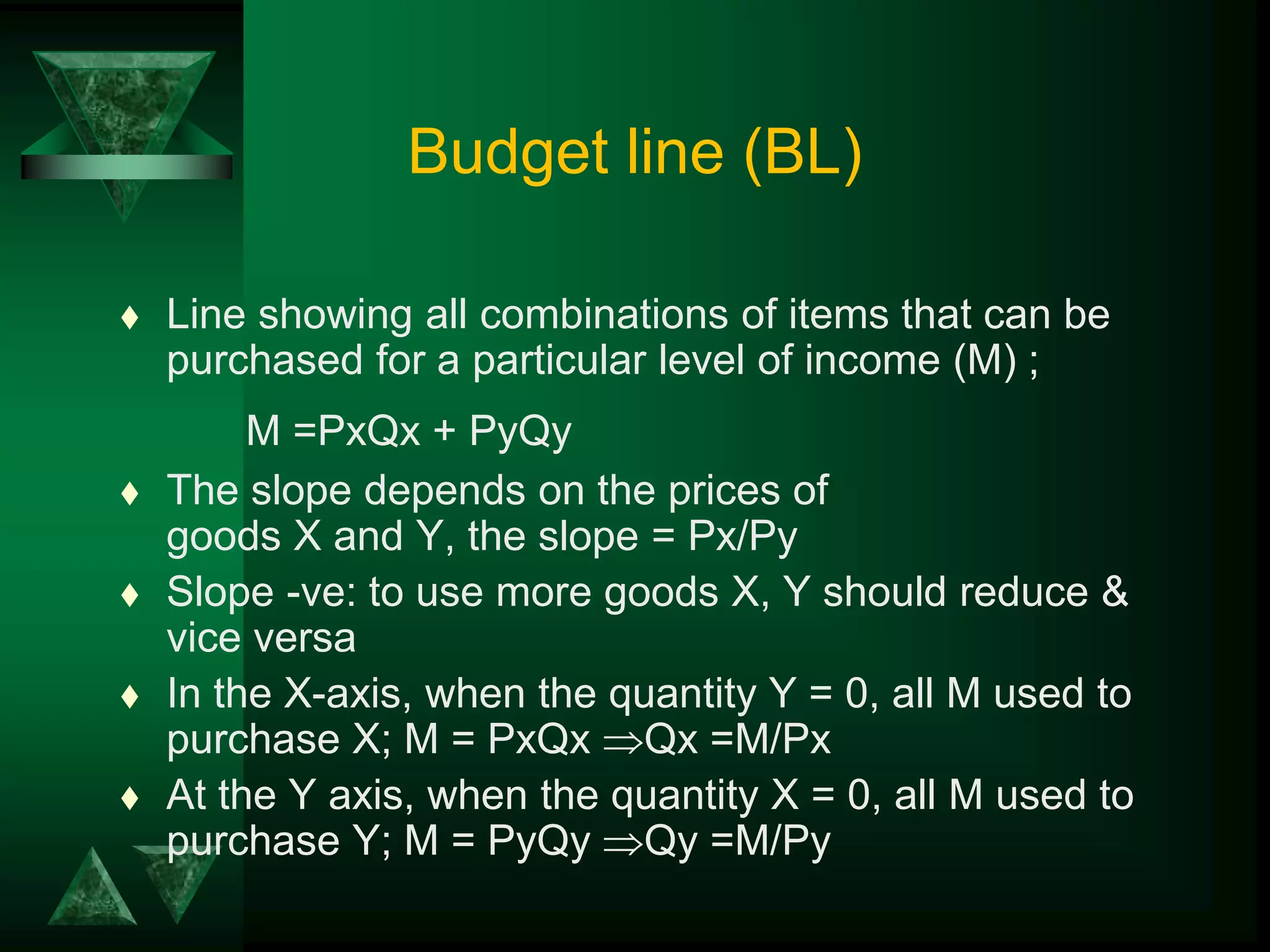
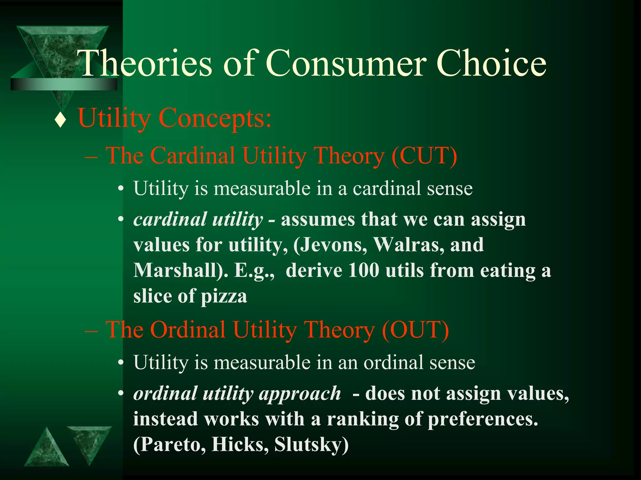
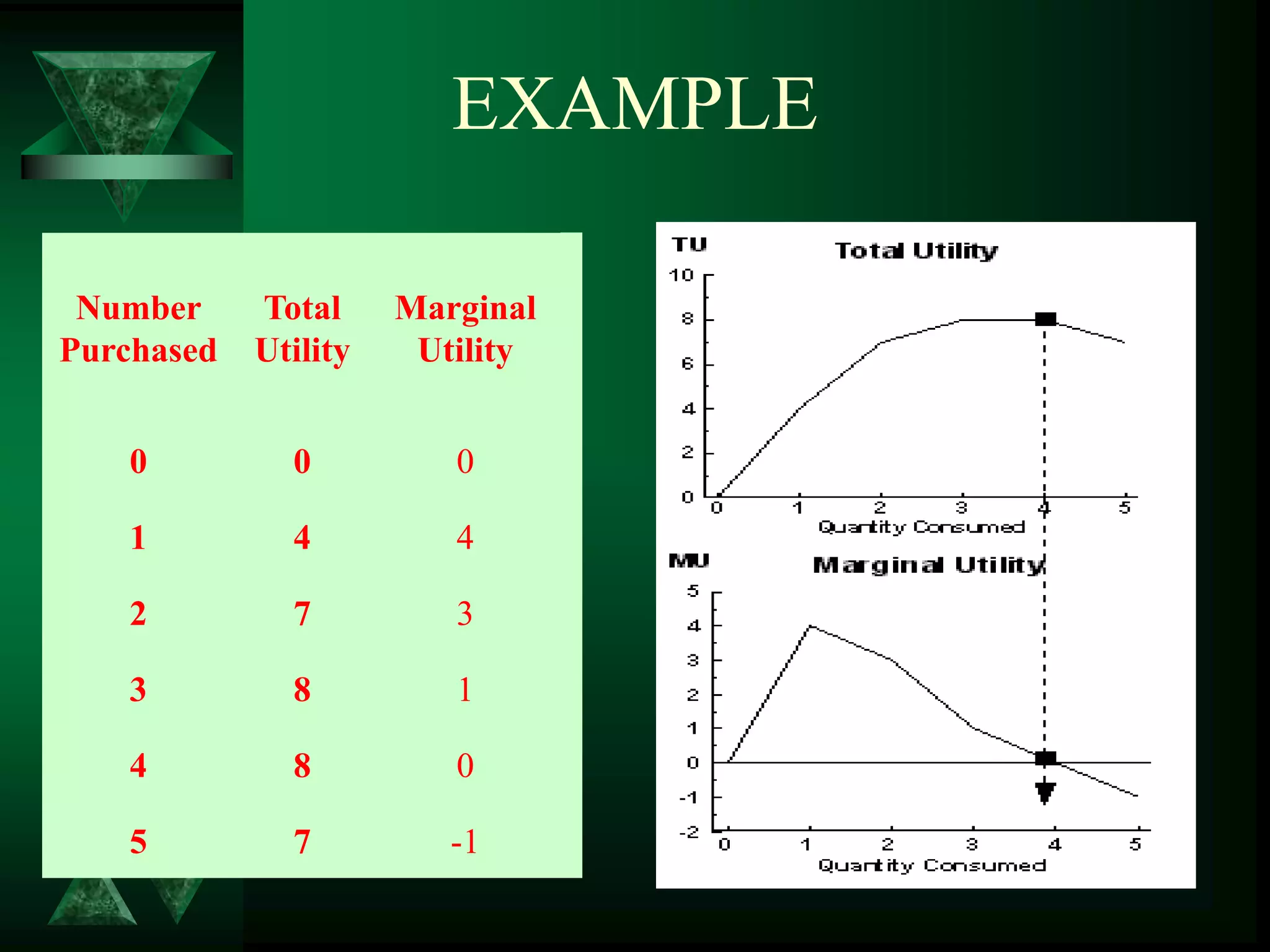
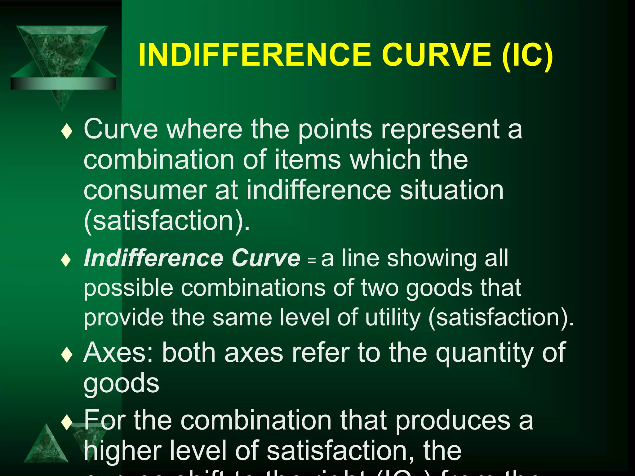
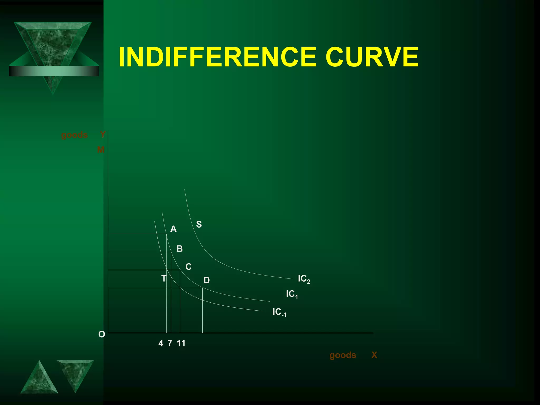
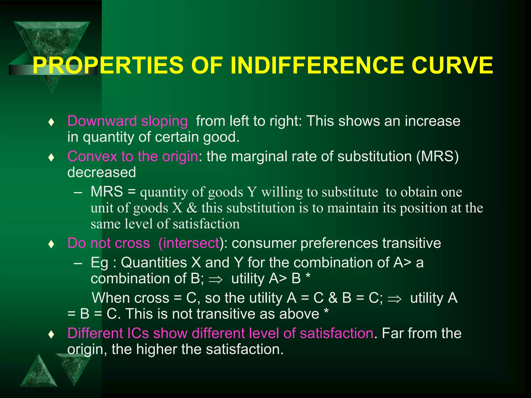
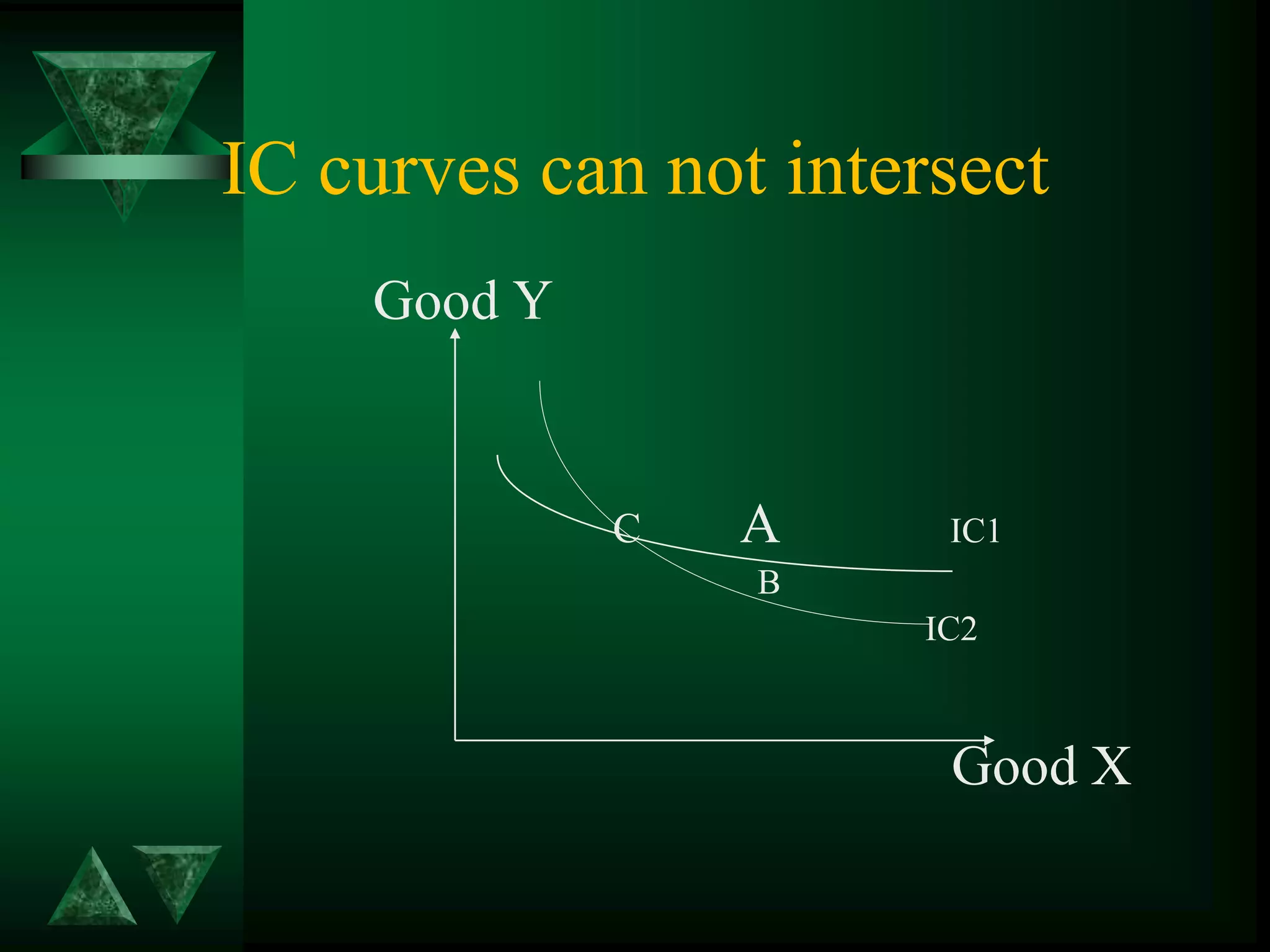
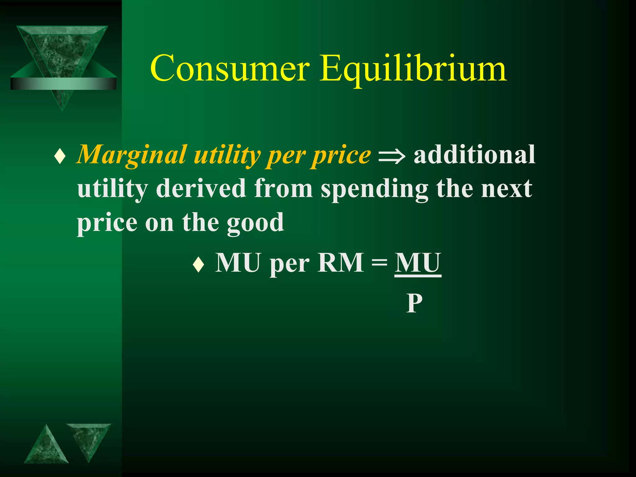
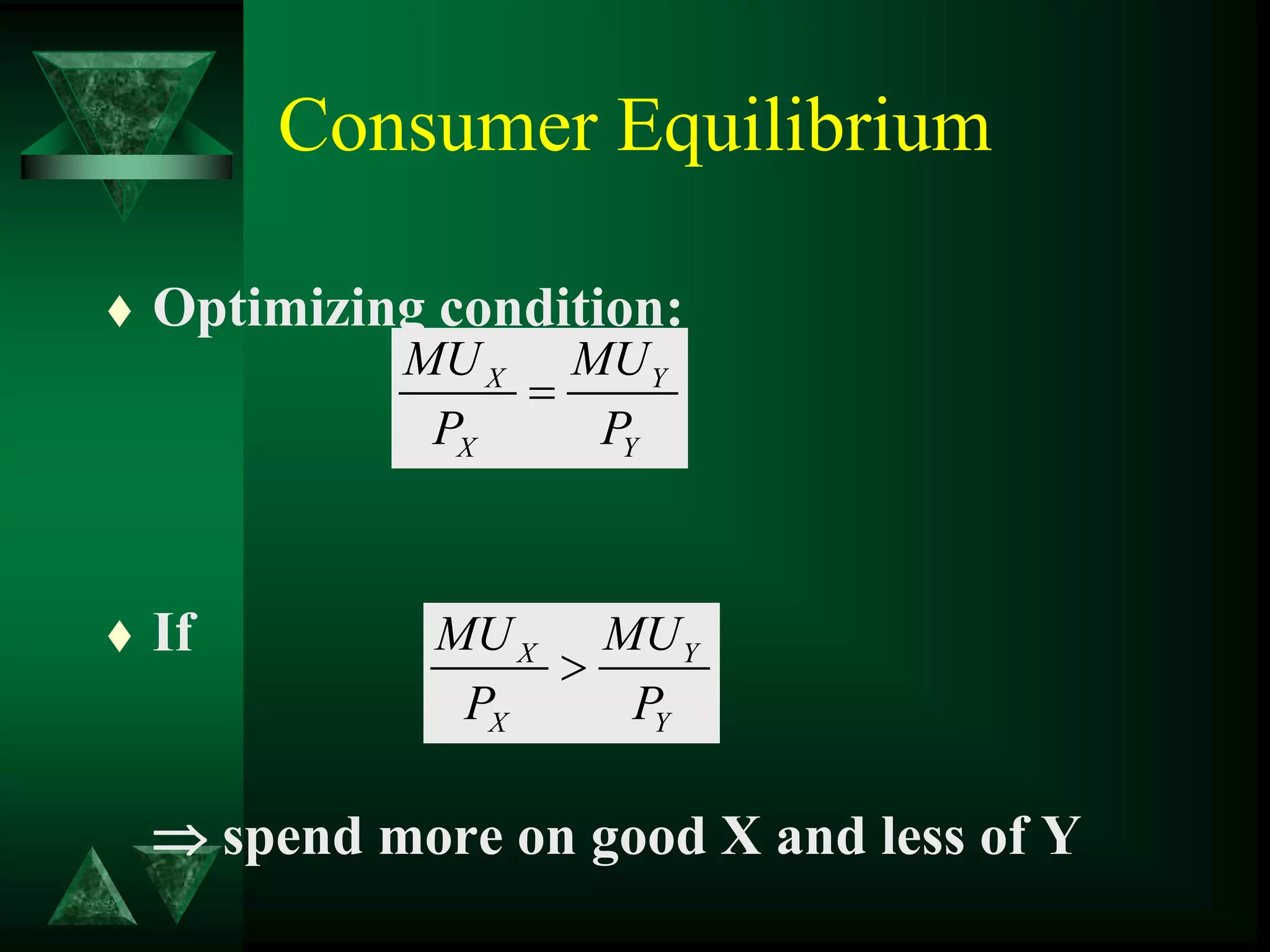
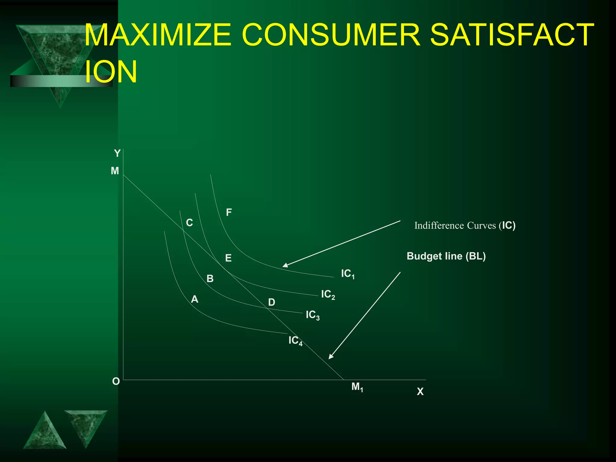
The document discusses theories of consumer behavior, including: - Consumers attempt to maximize utility given budget constraints by allocating income between goods. - Utility can be measured cardinally based on total and marginal utility, or ordinally using indifference curves. - Consumer equilibrium occurs where the indifference curve is tangent to the budget line, indicating equal marginal utility per dollar spent on each good. 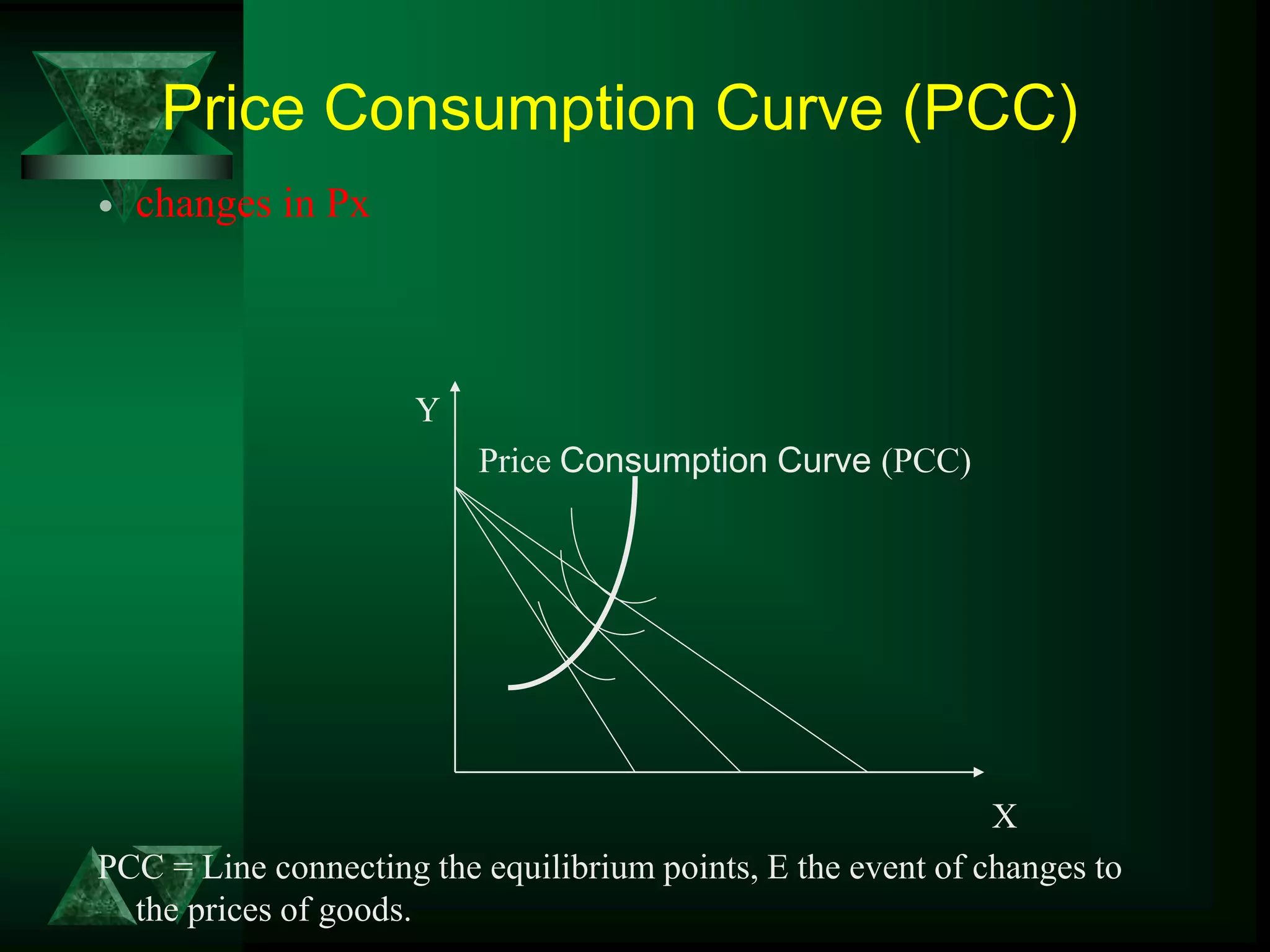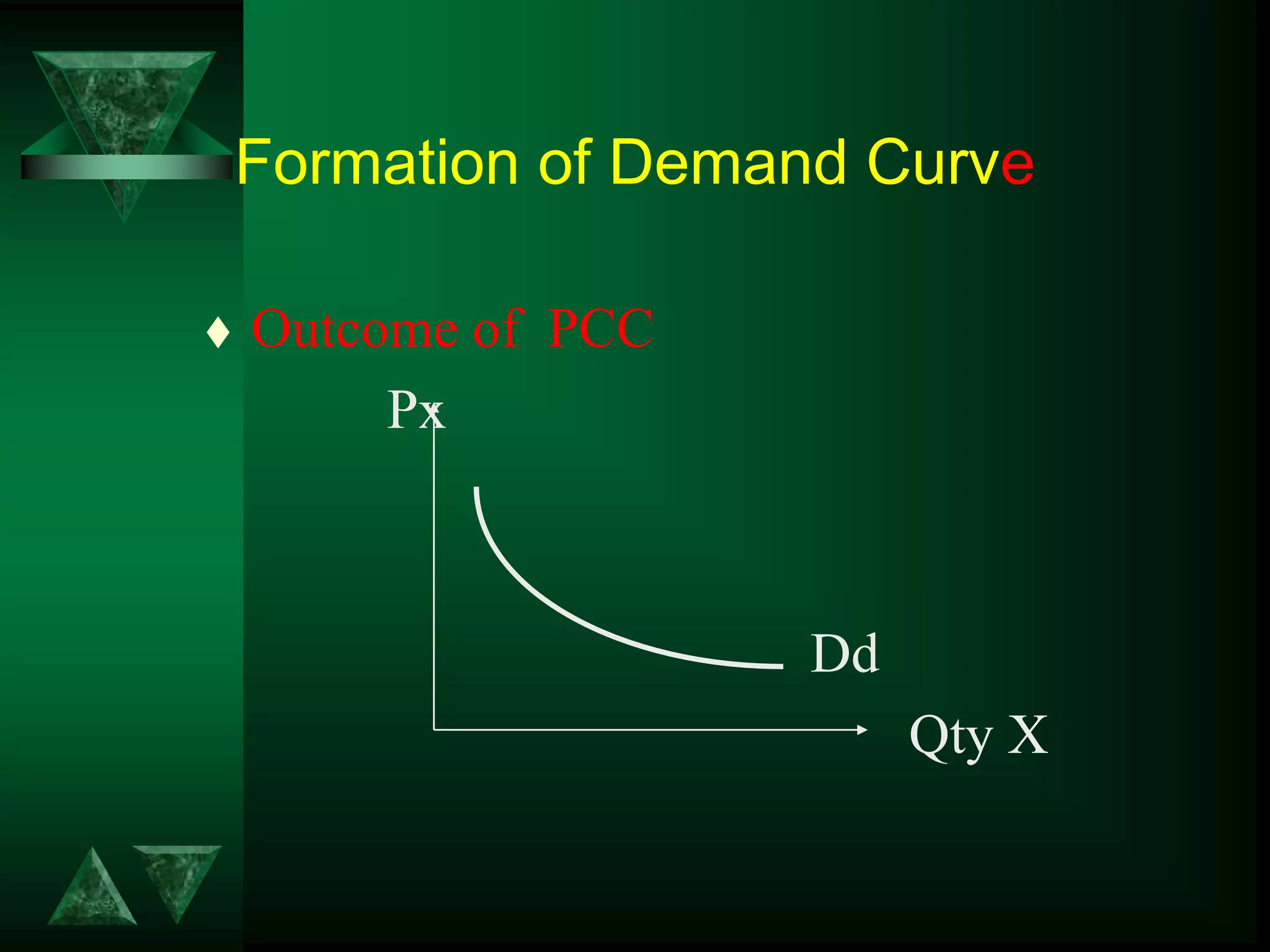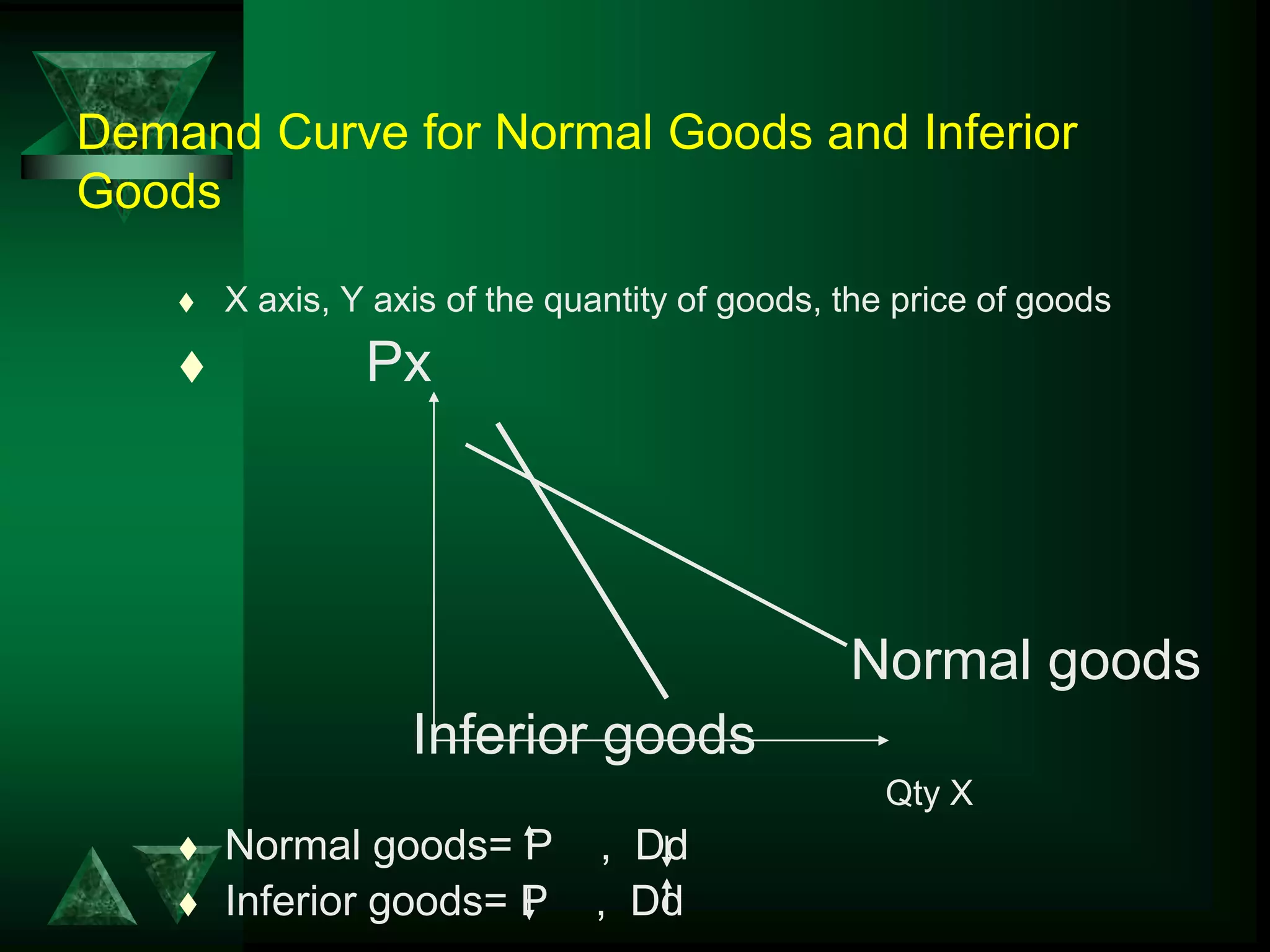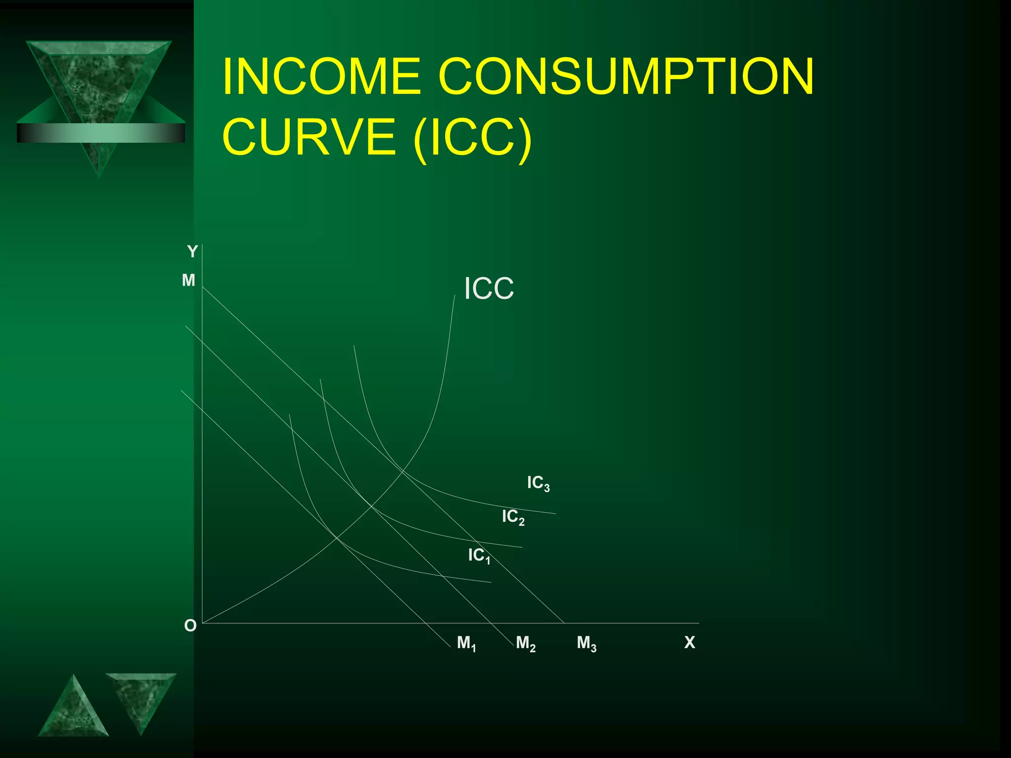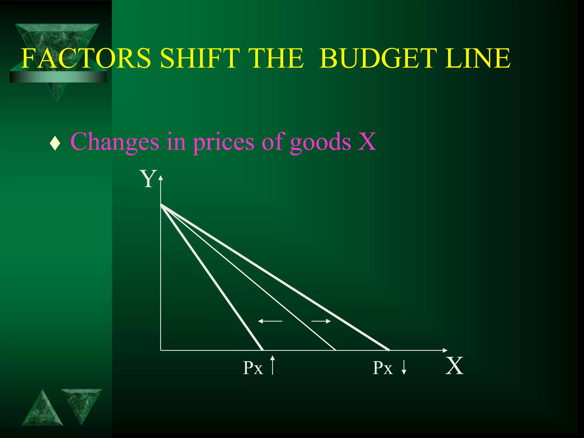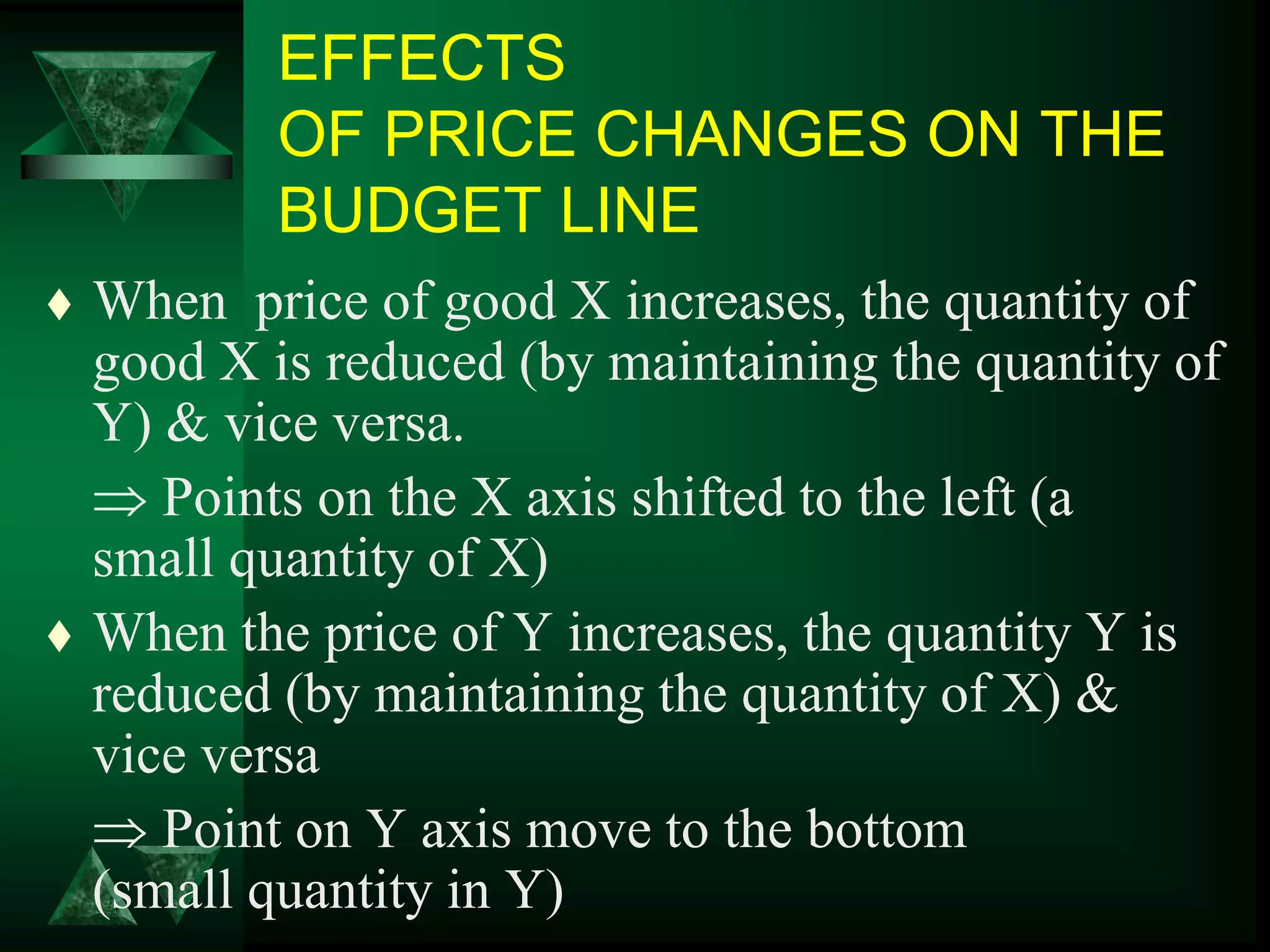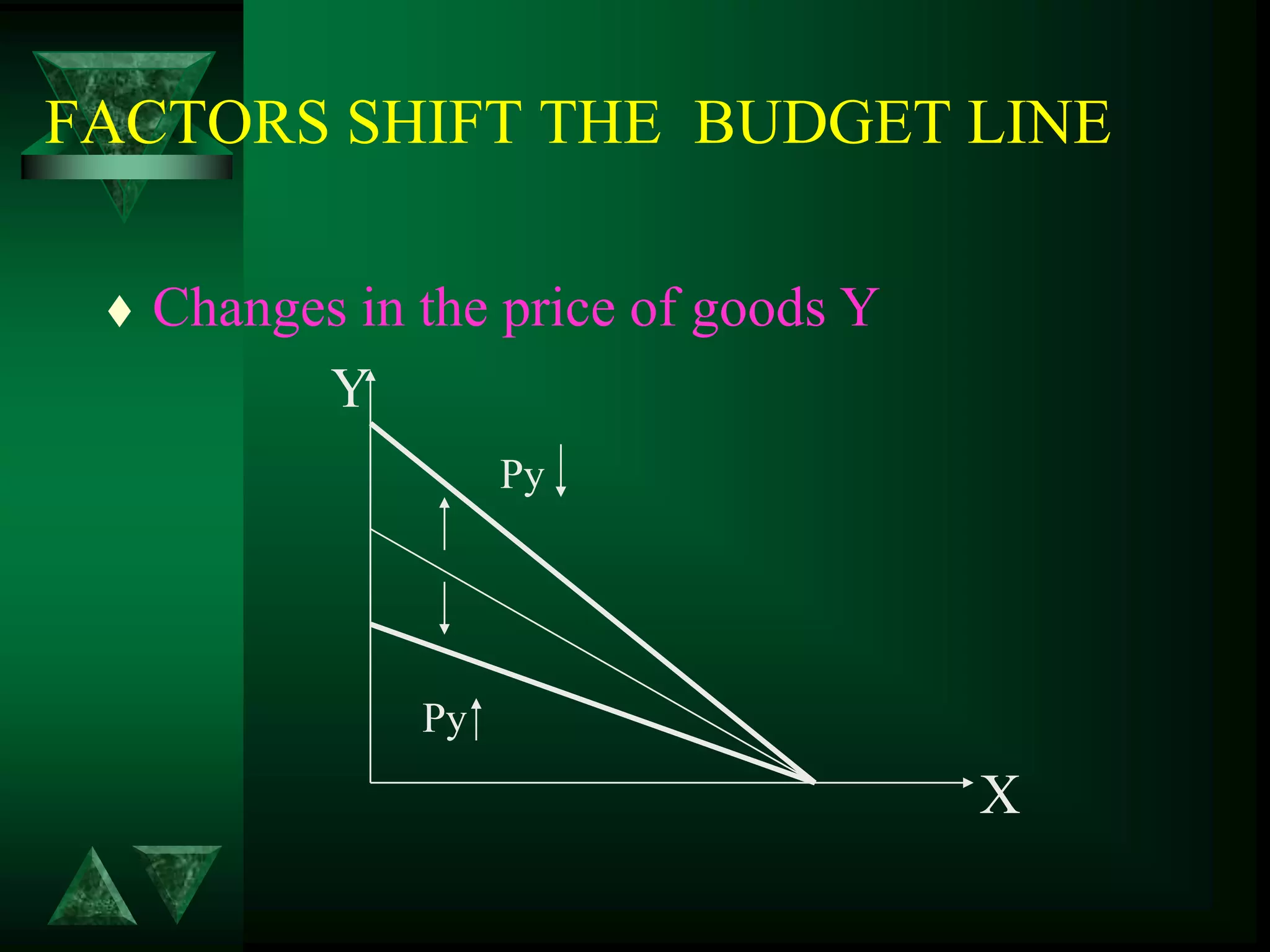- Changes in prices and income shift budget constraints, changing equilibrium and generating demand and income consumption curves.

1. The Theory of
Consumer Behavior
STANSLOUS K CHULU
DEPT OF ECONOMICS & BUSINESS STUDIES
FACULTY OF HUMANITIES

2. The Theory of Consumer
Behavior
The principle assumption upon which the
theory of consumer behavior and demand is
built is: a consumer attempts to allocate
his/her limited money income among
available goods and services so as to
maximize his/her utility (satisfaction).

3. Theory of Consumer Behavior
 Useful for understanding the demand side of
the market.
 Utility - amount of satisfaction derived from the
consumption of a commodity ….measurement
units  utils

4. Theories of Consumer Choice
 Utility Concepts:
– The Cardinal Utility Theory (CUT)
• Utility is measurable in a cardinal sense
• cardinal utility - assumes that we can assign
values for utility, (Jevons, Walras, and
Marshall). E.g., derive 100 utils from eating a
slice of pizza
– The Ordinal Utility Theory (OUT)
• Utility is measurable in an ordinal sense
• ordinal utility approach - does not assign values,
instead works with a ranking of preferences.
(Pareto, Hicks, Slutsky)

5. The Cardinal Approach
Nineteenth century economists, such as Jevons,
Menger and Walras, assumed that utility was
measurable in a cardinal sense, which means
that the difference between two measurement is
itself numerically significant.
UX = f (X), UY = f (Y), …..
Utility is maximized when:
MUX / MUY = PX / PY

6. The Cardinal Approach
 Total utility (TU) - the overall level of
satisfaction derived from consuming a good or
service
 Marginal utility (MU) additional satisfaction
that an individual derives from consuming an
additional unit of a good or service.
Formula :
MU = Change in total utility
Change in quantity
= ∆ TU
∆ Q

7. The Cardinal Approach
 Law of Diminishing Marginal Utility (Return) = As more
and more of a good are consumed, the process of
consumption will (at some point) yield smaller and
smaller additions to utility
 When the total utility maximum, marginal utility = 0
 When the total utility begins to decrease, the
marginal utility = negative (-ve)

8. EXAMPLE
Number
Purchased
Total
Utility
Marginal
Utility
0 0 0
1 4 4
2 7 3
3 8 1
4 8 0
5 7 -1

9. The Cardinal Approach
 TU, in general, increases
with Q
 At some point, TU can start
falling with Q (see Q = 5)
 If TU is increasing, MU > 0
 From Q = 1 onwards, MU is
declining  principle of
diminishing marginal utility
 As more and more of a
good are consumed, the
process of consumption will
(at some point) yield smaller
and smaller additions to
utility

10. Consumer Equilibrium
 So far, we have assumed that any amount
of goods and services are always
available for consumption
 In reality, consumers face constraints
(income and prices):
– Limited consumers income or budget
– Goods can be obtained at a price

11. Some simplifying assumptions
 Consumer’s objective: to maximize
his/her utility subject to income
constraint
 2 goods (X, Y)
 Prices Px, Py are fixed
 Consumer’s income (I) is given

12. Consumer Equilibrium
 Marginal utility per price  additional
utility derived from spending the next
price on the good
 MU per RM = MU
P

13. Consumer Equilibrium
 Optimizing condition:
 If
 spend more on good X and less of Y
X Y
X Y
MU MU
P P

X Y
X Y
MU MU
P P


14. Numerical Illustration
Qx TUX MUX
MUx
Px
QY TUY MUY
MUy
Py
1 30 0 0 1 50 0 0
2 39 9 4.5 2 105 55 5.5
3 45 6 3 3 148 43 4.3
4 50 5 2.5 4 178 30 3
5 54 4 2 5 198 20 2
6 56 2 1 6 213 15 1.5

15. Simple Illustration
 Suppose: X = fish
Y = Meat
 Assume: PX = 2
PY = 10

16. Cont.
 2 potential optimum positions
 Combination A:  X = 3 and Y = 4
– TU = TUX + TUY = 45 + 178 = 223
 Combination B:  X = 5 and Y = 5
– TU = TUX + TUY = 54 + 198 = 252

17. Cont.
 Presence of 2 potential equilibrium
positions suggests that we need to
consider income. To do so let us examine
how much each consumer spends for
each combination.
 Expenditure per combination
– Total expenditure = PX X + PY Y
– Combination A: 3(2) + 4(10) = 46
– Combination B: 5(2) + 5(10) = 60

18. Cont.
 Scenarios:
– If consumer’s income = 46, then the
optimum is given by combination A.
.…Combination B is not affordable
– If the consumer’s income = 60, then the
optimum is given by Combination
B….Combination A is affordable but it
yields a lower level of utility

19. The Ordinal Approach
Economists following the lead of Hicks,
Slutsky and Pareto believe that utility is
measurable in an ordinal sense--the utility
derived from consuming a good, such as X,
is a function of the quantities of X and Y
consumed by a consumer.
U = f ( X, Y )

20. Cont.
 Ordinal Utility Theory (TUO)
– Can be measured in qualitative,
not quantitative, but only lists
the main options (indifference curves & budget
line).
 Rational human beings will choose
to maximize the utility by selecting the
highest utility
 Difference consumers, difference utilities.

21. INDIFFERENCE CURVE (IC)
 Curve where the points represent a
combination of items which the
consumer at indifference situation
(satisfaction).
 Indifference Curve = a line showing all
possible combinations of two goods that
provide the same level of utility (satisfaction).
 Axes: both axes refer to the quantity of
goods
 For the combination that produces a
higher level of satisfaction, the

22. INDIFFERENCE CURVE
Y
O
goods
7
Y
O
X
IC2
IC1
M
IC-1
11
4
goods
S
A
B
C
D
T

23. PROPERTIES OF INDIFFERENCE CURVE
 Downward sloping from left to right: This shows an increase
in quantity of certain good.
 Convex to the origin: the marginal rate of substitution (MRS)
decreased
– MRS = quantity of goods Y willing to substitute to obtain one
unit of goods X & this substitution is to maintain its position at the
same level of satisfaction
 Do not cross (intersect): consumer preferences transitive
– Eg : Quantities X and Y for the combination of A> a
combination of B;  utility A> B *
When cross = C, so the utility A = C & B = C;  utility A
= B = C. This is not transitive as above *
 Different ICs show different level of satisfaction. Far from the
origin, the higher the satisfaction.

24. IC curves can not intersect
Good Y
C A IC1
B
IC2
Good X

25. Budget line (BL)
 Line showing all combinations of items that can be
purchased for a particular level of income (M) ;
M =PxQx + PyQy
 The slope depends on the prices of
goods X and Y, the slope = Px/Py
 Slope -ve: to use more goods X, Y should reduce &
vice versa
 In the X-axis, when the quantity Y = 0, all M used to
purchase X; M = PxQx Qx =M/Px
 At the Y axis, when the quantity X = 0, all M used to
purchase Y; M = PyQy Qy =M/Py

26. FACTORS SHIFT THE BUDGET LINE
 Changes in prices of goods X
Y
Px Px X

27. EFFECTS
OF PRICE CHANGES ON THE
BUDGET LINE
 When price of good X increases, the quantity of
good X is reduced (by maintaining the quantity of
Y) & vice versa.
 Points on the X axis shifted to the left (a
small quantity of X)
 When the price of Y increases, the quantity Y is
reduced (by maintaining the quantity of X) &
vice versa
 Point on Y axis move to the bottom
(small quantity in Y)

28. FACTORS SHIFT THE BUDGET LINE
 Changes in the price of goods Y
Y
Py
Py
X

29. FACTORS SHIFT THE BUDGET LINE
 Changes in income
Y
I
I
 X

30. EFFECTS OF INCOME
CHANGES ON THE
BUDGET LINE
 When M increases, QX and QY can be
bought even more, a point on the X
axis shifted to the right & a point on
the Y axis move on; & vice
versa when M decreases.

31. CONSUMER EQUILIBRIUM
 With income (M) some combination
of goods that consumers choose the highest
satisfaction
 Satisfied the
same curves and budget lines are
connected
 The point where the curve IC and
BL tangent
 Slope IC = BL
 Consumer choice influenced by income

32. MAXIMIZE CONSUMER SATISFACT
ION
F
E
B
A D
C
Y
O
X
IC1
IC2
IC3
IC4
M1
M
Budget line (BL)
Indifference Curves (IC)

33. EXAMPLE
a) A consumer spends all her income on food and
clothing. At the current prices of Pf = K10 and Pc = K5,
she maximized her utility by purchasing 20 units of
food and 50 units of clothing.
 i.What is the consumer’s income? [2 marks]
 ii.What is the consumer’s marginal rate of substitution
of food for clothing at the equilibrium position? [2
marks]

34. Price Consumption Curve (PCC)
 changes in Px
Y
Price Consumption Curve (PCC)
X
PCC = Line connecting the equilibrium points, E the event of changes to
the prices of goods.

35. Formation of Demand Curve
 Outcome of PCC
Px
Dd
Qty X

36. Demand Curve for Normal Goods and Inferior
Goods
 X axis, Y axis of the quantity of goods, the price of goods
 Px
Normal goods
Inferior goods
Qty X
 Normal goods= P , Dd
 Inferior goods= P , Dd

37. INCOME CONSUMPTION CURVE
(ICC)
 If a fixed price and income increases, the
budget line shifts to the right,
thus shifting the equilibrium point higher.
 Equilibrium point some
income items associated with the line -
can be income consumption curve (ICC).
 ICC shows the points for the combination
of goods that can be purchased when
income change and fixed in price.

38. INCOME CONSUMPTION
CURVE (ICC)
Y
O
X
IC3
IC2
M3
M
IC1
M2
M1
ICC

39. ENGEL CURVE
O
X
20
M
16
12 22
40
Engel curve for x
20
10
30

40. ENGEL CURVE
 Relationship of income to the
quantity of an item
 Retrieved from ICC
 Get a quantity of goods X or Y that can
be purchased goods with an income
 Plot the quantity
of X or Y against income
 Linking income changes with changes
in demand for goods at a fixed price

41. Engel curve for luxury goods and
normal goods
M
X
Normal goods
Luxury goods
O

42. Conclusion
 To CB showing how it provides users a combination of sources of income
for many goods /services
 There are two types of utility theory:
– Cardinal  TU and MU
– Ordinal  curve IC and BL
 Equilibrium and utility maximization can be either TUC or TUO
 Equilibrium points of connection to produce PCC (change IN PRICE)
and ICC (change in income)
 Displaying Publication = PCC curve DD & ICC = Engel curve (EC)
 The types of goods obtained displaying income or price changes.

43. Thank You