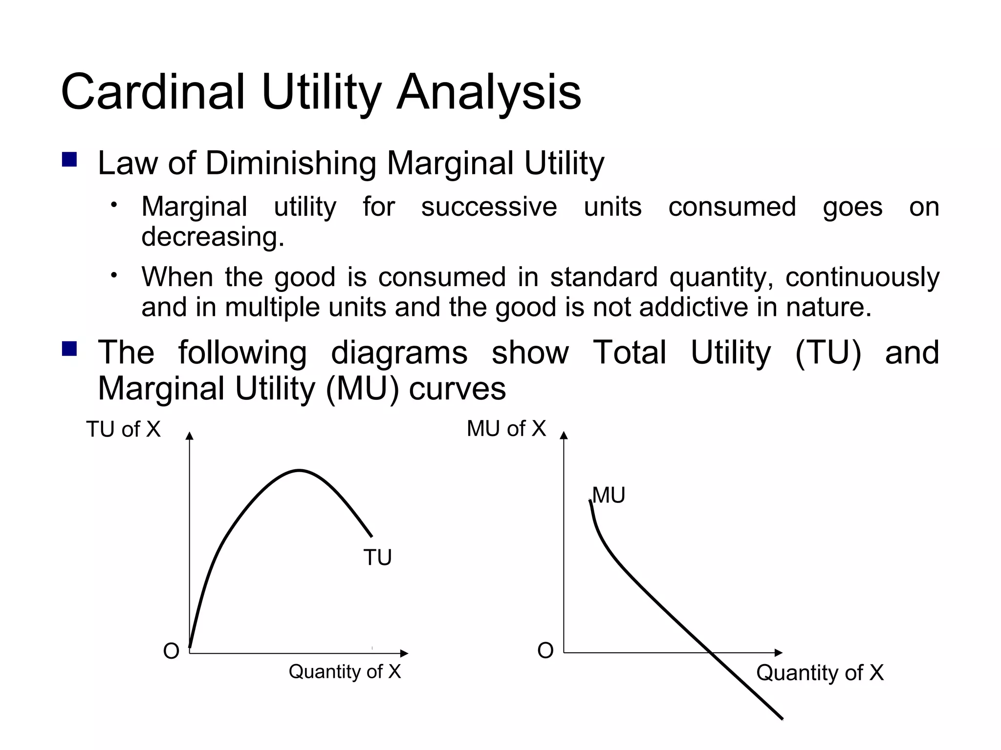
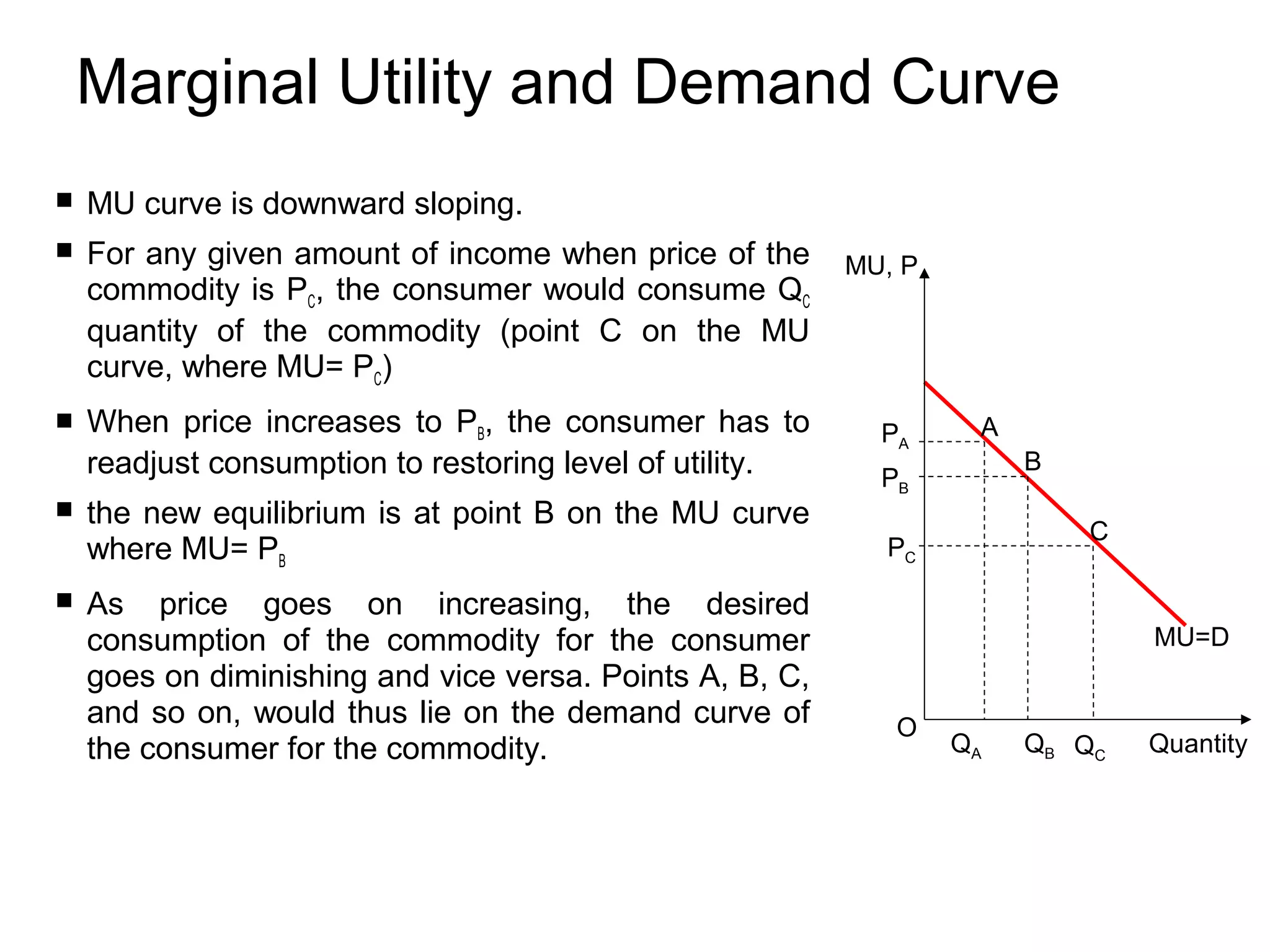
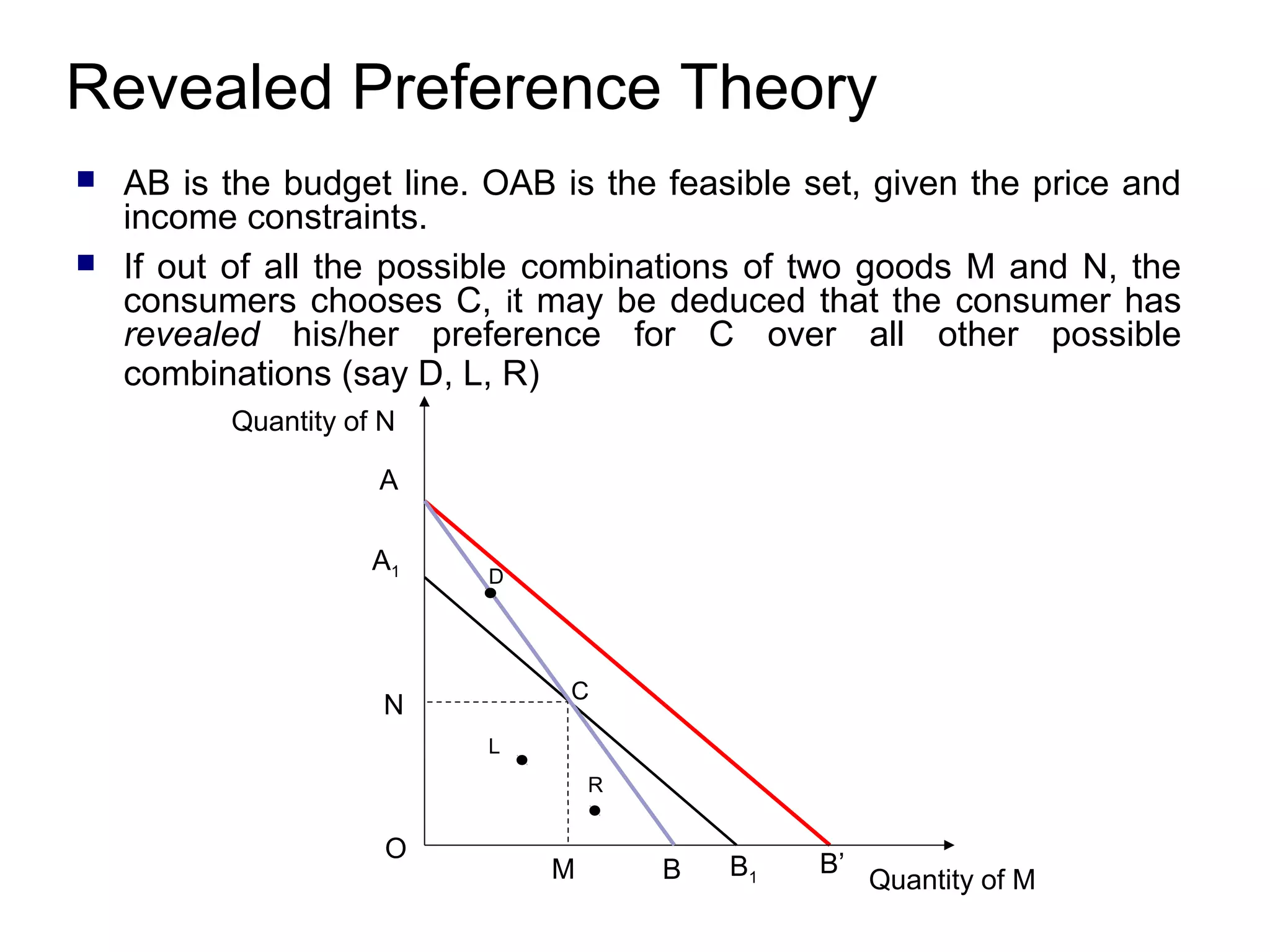
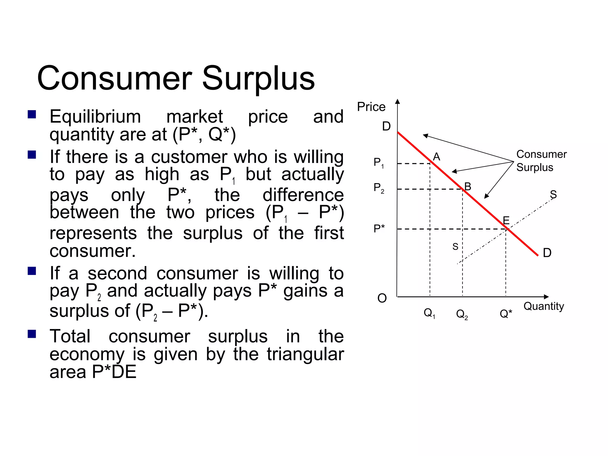
Consumer preferences and choices are based on the utility or satisfaction derived from consuming goods. There are two views on utility - the cardinal view which measures utility in quantifiable units, and the ordinal view which ranks preferences. The law of diminishing marginal utility and equimarginal utility principle explain how consumption changes with price. Indifference curves illustrate preferences graphically on a budget constraint. Consumer equilibrium maximizes utility subject to the budget. Revealed preference theory observes consumer behavior. Consumer surplus measures the benefit consumers gain when price is below what they are willing to pay.

1. Chapter 4
Consumer Preferences
and Choice

2. Lecture plan









Objectives
Consumer Choice
Cardinal Utility Analysis
Marginal Utility and Demand Curve
Ordinal Utility Analysis
Diminishing Marginal Rate of Substitution
Consumer’s Equilibrium
Revealed Preference Theory
Consumer Surplus

3. Objectives





To introduce the crux of consumer behaviour,
choices and preferences.
To explain the nuances of utility analysis,
marginal utility, total utility and law of
diminishing marginal utility.
To explain the difference between cardinal and
ordinal utility analyses of consumer behaviour.
To discuss how consumer equilibrium is
attained subject to budget constraint.
To illustrate the concept of consumer surplus
and its application in decision making.

4. Consumer Choice


Given the prices of different commodities,
consumers decide on the quantities of these
commodities according to their paying capacity,
and tastes and preferences.
Consumers’ choices, tastes and preferences
rests on the following assumptions:
 Completeness:
A consumer would be able to state
own preference or indifference between two distinct
baskets of goods.
 Transitivity: An individual consumer’s preferences
are always consistent.
 Non-satiation: A consumer is never satiated
permanently. More is always wanted; if “some” is
good, “more” of the good is better.

5. Consumer Choice

Commodities are desired because of their utility
 Utility
is the attribute of a commodity to satisfy or
satiate a consumer’s wants
 Utility is the satisfaction a consumer derives from
consumption of a commodity

Mathematically: utility is the function of the
quantities of different commodities consumed:
U= f(m1, n1, r1)

6. Cardinal Utility Analysis


Marshall and Jevons opined that Utility is a cardinal
concept and is measurable (in utils) like any other physical
commodity
Total Utility (TU)


Sum total of utility levels out of each unit of a commodity
consumed within a given period of time
Marginal Utility (MU)


Change in total utility due to a unit change in the commodity
consumed within a given period of time.
dTU
MU=TUn -TUn-1 or MU=
dQ

7. Cardinal Utility Analysis

Law of Equimarginal Utility
 Marginal
utilities of all commodities should be equal
 The consumer has to distribute his/her income on
different commodities so that utility derived from
last unit of each commodity is equal for all other
commodities in the consumption basket.

Mathematically:
MU M MU N
=
= ... = MU I
PM
PN

8. Cardinal Utility Analysis

Law of Diminishing Marginal Utility
•
•

Marginal utility for successive units consumed goes on
decreasing.
When the good is consumed in standard quantity, continuously
and in multiple units and the good is not addictive in nature.
The following diagrams show Total Utility (TU) and
Marginal Utility (MU) curves
MU of X
TU of X
MU
TU
O
Quantity of X
O
Quantity of X

9. Marginal Utility and Demand Curve

MU curve is downward sloping.

For any given amount of income when price of the
commodity is PC, the consumer would consume QC
quantity of the commodity (point C on the MU
curve, where MU= PC)

When price increases to PB, the consumer has to
readjust consumption to restoring level of utility.


the new equilibrium is at point B on the MU curve
where MU= PB
As price goes on increasing, the desired
consumption of the commodity for the consumer
goes on diminishing and vice versa. Points A, B, C,
and so on, would thus lie on the demand curve of
the consumer for the commodity.
MU, P
PA
A
B
PB
C
PC
MU=D
O
QA
QB QC
Quantity

10. Ordinal Utility Analysis

Edgeworth, Fisher and others negate the physical
measurement of utility.

Utility is not additive but comparative.
Indifference Curve Analysis (J.R. Hicks and R.G.D. Allen )
 Indifference curve: Locus of points which show the different
combinations of two commodities among which the consumer is
indifferent, i.e. derives same utility.
 Since all these points render equal utility to the consumer, an
indifference curve is also known as an isoutility (“iso” meaning
equal) curve.
 Indifference map: group of indifference curves


A consumer is able to rank different combinations of the
commodities in order of preference or indifference.

11. Properties of Indifference Curves
Indifference curves are downward
sloping.
•



This is because of the assumption of
non-satiation.
Higher
indifference
curve
represents higher utility.
Indifference curves can never
intersect.
Indifference curves are convex to
the origin.
•
This is because two goods cannot be
perfect substitutes of each other.
Y
A
Good Y

O
B
C
D
IC1
Good X
IC2
X

12. Exceptional Shapes of Indifference
Curves
QY
Perfect Substitutes
O
QY
O
QX
Irrational
Behaviour
QX
Perfect Complements
QY
O
QY
QX
Social Bads
O
QX

13. Diminishing Marginal Rate of
Substitution

MRS is the proportion of one good (M) that the consumer would
be willing to give up for more of another (N)

MRS is the ratio between rates of change in M and N, down the
indifference curve :
∆N …..(1)
MRS MN = −
∆M

To increase consumption of M, the consumer has to reduce
consumption of N and hence the negative sign. MRSMN goes on
diminishing as we move down the indifference curve.

Gain in utility due to consumption of more units of one commodity
must be equal to the loss in utility due to consumption of less units
of the other commodity
MU M
MU M
MU N
= − ∆N
MU N
∆M
= MRS MN
…..(2)
…..(3)

14. Consumer’s Equilibrium
 Consumer
would reach equilibrium point, i.e. highest level
of
satisfaction given all constraints at the highest
indifference curve he/she can reach.
 Budget
line of a consumer, consists of all possible
combinations of the two commodities that the consumer
can purchase with a limited budget:
 Budget
constraint depends upon income of the consumer
and prices of the commodities in the consumption basket.
Mathematically
PM.QM+PN.QN=I
(Where PM is price of commodity M, QM quantity of M, PN price of N, QN
quantity of M and I is income of the consumer.

15. Consumer’s Equilibrium

Conditions for consumer’s equilibrium:



Consumer spends all income in buying the two commodities;
hence point of equilibrium will always lie on the budget line.
Point of equilibrium will always be on the highest possible
indifference curve the consumer can reach with the given budget
line.
Consumer is able to maximize utility at a point where the budget line
is tangent to an indifference curve
This is the highest possible curve attainable by the consumer,
subject to budget constraint.
Budget line may


shift either upwards or downwards due to any change in income of the
consumer while price of the commodities remaining same
 Swivel at one point when price of one of the commodities changes, while
income and price of other commodity remain same.


16. Consumer’s Equilibrium




Feasible set is the area OAB, Quantity of N
and area beyond budget line
A
AB is infeasible area; therefore
IC4 is beyond reach of the
consumer.
Equilibrium is attained at point
E where the AB is tangent to
curve IC3 (highest attainable
indifference curve).
QN
C
E
Point C and B are attainable
but on lower indifference
curve.
Equilibrium
quantities
of
commodities M and N are QM
and QN.
IC4
D
IC3
IC2
IC1
O
QM
B
Quantity of M

17. Revealed Preference Theory





Indifference curves analysis had limitations in terms of its highly
theoretical structure and simplifying assumptions.
Samuelson came up with an approach to assessing consumer
behaviour and introduced the term ‘revealed preference’. The basic
hypothesis of the theory is ‘choice reveals preference’.
Demand for a commodity by a consumer can be ascertained by
observing the actual behaviour of the consumer in the market in
various price and income situations.
This gives us a demand curve for an individual consumer on the
basis of observed behaviour.
Demand for any good (or basket of goods) is known to always
increase when money income alone rises hence it must shrink
when price alone rises.

18. Revealed Preference Theory


AB is the budget line. OAB is the feasible set, given the price and
income constraints.
If out of all the possible combinations of two goods M and N, the
consumers chooses C, it may be deduced that the consumer has
revealed his/her preference for C over all other possible
combinations (say D, L, R)
Quantity of N
A
A1
D
C
N
L
R
O
M
B
B1
B’
Quantity of M

19. Consumer Surplus



The difference between the price consumers are
willing to pay and what they actually pay is called
consumer surplus.
Individual consumer surplus measures the gain
that a consumer makes by purchasing a product
at a price lower than what he/she had expected
to pay.
In a market the total consumer surplus measures
the gain to the society due to the existence of a
market transaction.

20. Consumer Surplus




Equilibrium market price and
quantity are at (P*, Q*)
If there is a customer who is willing
to pay as high as P1 but actually
pays only P*, the difference
between the two prices (P1 – P*)
represents the surplus of the first
consumer.
If a second consumer is willing to
pay P2 and actually pays P* gains a
surplus of (P2 – P*).
Total consumer surplus in the
economy is given by the triangular
area P*DE
Price
D
P1
Consumer
Surplus
A
B
P2
S
E
P*
S
D
O
Q1
Q2
Q*
Quantity

21. Summary
Utility is the measure of satisfaction a consumer derives from
consumption of a commodity; it is an attribute of a commodity to satisfy
a consumer’s needs. According to cardinal school, utility is measurable
like any other physical commodity.
 As per law of diminishing marginal utility, as you one consumes more
and more units of a commodity, total utility would goes on increasing,
but at a diminishing rate.
 As per law of equimarginal utility, a consumer will maximize utility when
the marginal utility of the last unit of money spent on each commodity is
equal to the marginal utility of the last unit of money spent on any other
commodity.
 According to ordinal school, utility cannot be measured in physical
units; it is possible to rank utility derived from various commodities.
 Indifference curves are downward sloping and convex to the origin; a
higher indifference curve would represent higher utility and two
indifference curves do not intersect each other.


22. Summary





Marginal Rate of Substitution (MRS) shows the amount of a
good that a consumer would be willing to give up for an
additional unit of another commodity.
Budget constraint to the consumer includes income of the
consumer and prices of the commodities in the consumption
basket. A change in any of these constraints would lead to a
shift in the budget line. Such a shift can be of three types:
upwards, downwards and swivelling.
The consumer will be at equilibrium at a point where the budget
line is tangent to the highest attainable indifference curve.
According to the theory of revealed preferences, demand for a
commodity by a consumer can be ascertained by observing the
buying pattern of the consumer.
Consumer surplus is equal to the difference between the price a
consumer is willing to pay and the price he/she actually pays for
a commodity.