This document provides an introduction to Microsoft Excel. It begins with opening Excel and navigating within workbooks and worksheets. It describes entering different types of data like numbers, text, formulas. It discusses selecting cells, entering and editing data, copying and moving data using fill handle. It also covers saving workbooks in compatibility mode to allow opening in older Excel versions. The document is presented by Abdulbasit H. Mhdi and contains guidance, instructions and screenshots to explain key Excel concepts.
Presentation introduction by Abdulbasit H. Mhdi, covering basic opening methods for Microsoft Excel.
Overview of Excel's functionality related to numbers, workbooks, and worksheets. It explains workbooks management.
Description of the Excel 2007 interface, including the Ribbon layout and key components of the window.
Detailed layout explanation of tables, rows, columns, and the Quick Access Toolbar functionality.
Instructions on opening, closing, and navigating through workbooks and worksheets in Excel.
Methods for selecting cells, rows, columns, and multiple areas within a worksheet using mouse or keyboard.
Guidance on entering data into Excel and creating or opening new workbooks.
Instructions for deleting, moving, and copying data in Excel cells.
Explains using Excel's AutoFill feature for data series replication.
Instruction on saving Excel files and ensuring compatibility with older versions.
Methods for editing cell data directly, highlighting the difference between edit mode and data entry mode.
Instructions for inserting and deleting cells, rows, and columns to restructure worksheets.
Instructions on inserting, deleting, and renaming worksheets in Excel.
Explains formatting cells, including width adjustments, hiding data, and keeping headings visible.
Introduction to creating formulas, using operators, and evaluating arithmetic expressions.
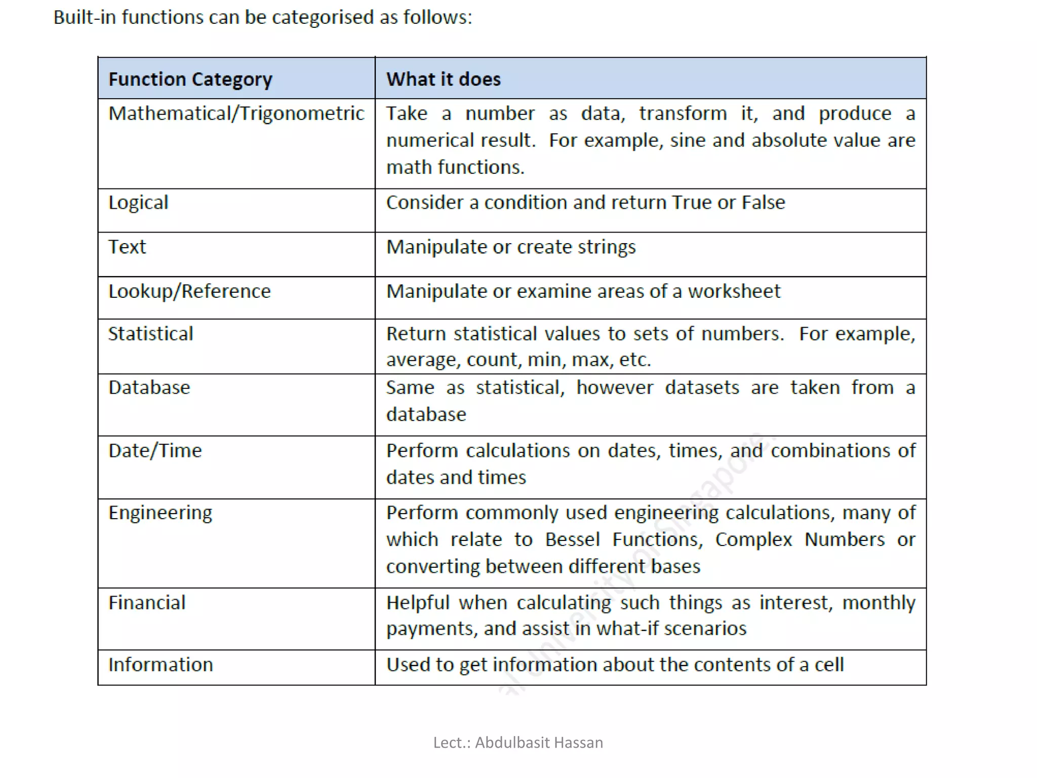
Overview of built-in functions and how to apply them in Excel for calculations.
Instructions for complex formulas, including nested functions and logical expressions like IF.
Details on using trigonometric and exponential functions within Excel.
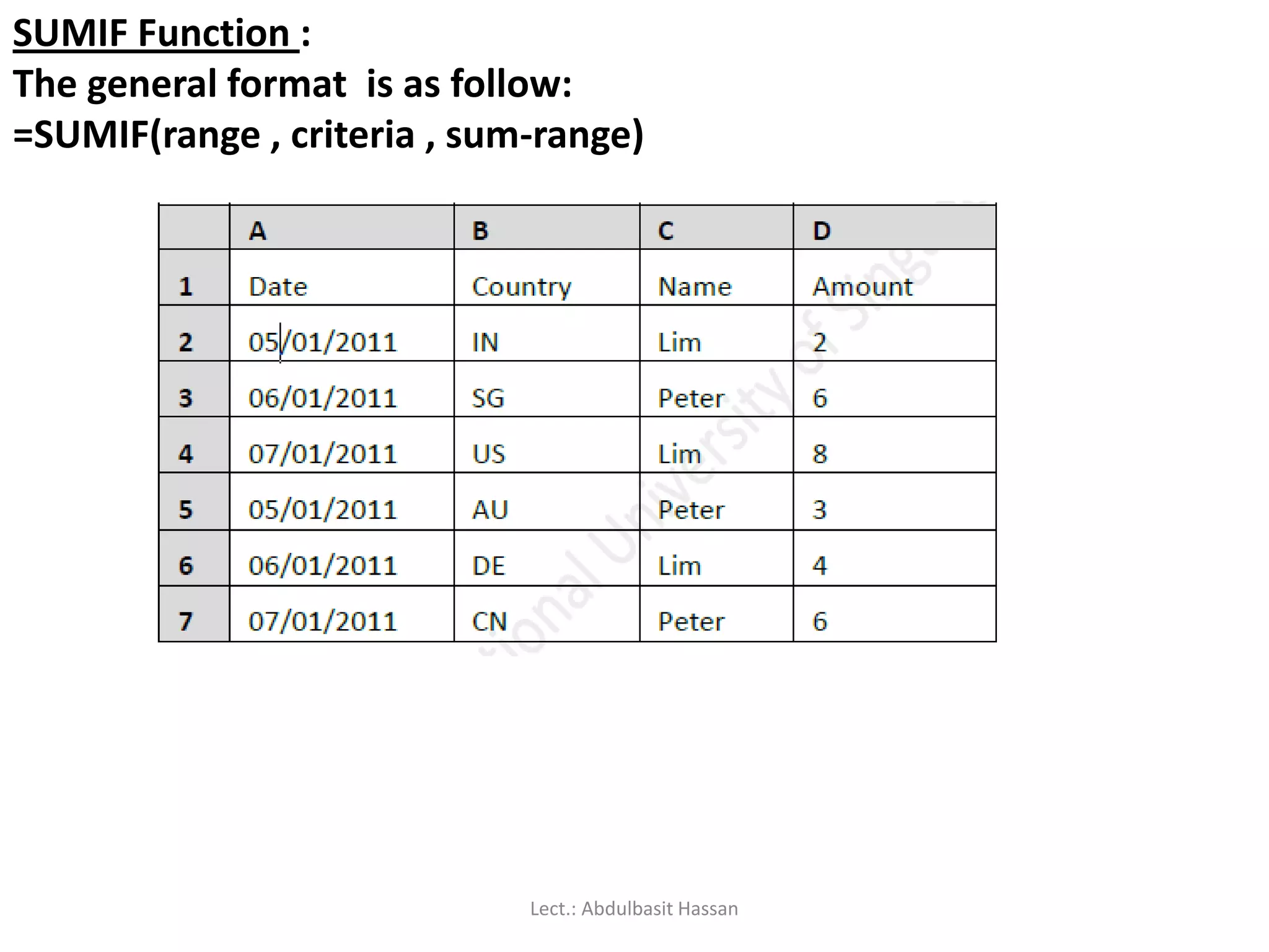
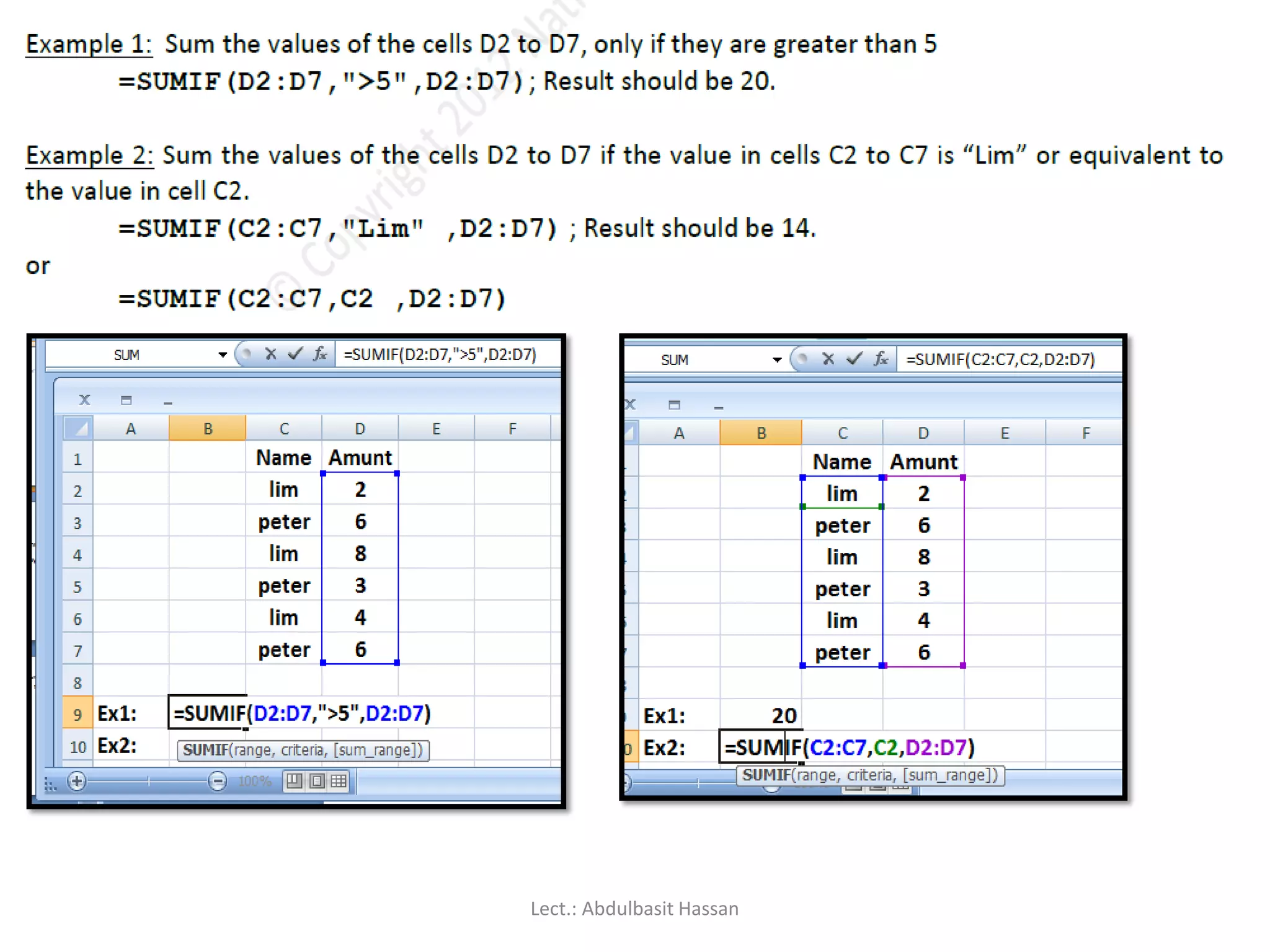
Instructions on SUMIF function and applying conditions in calculations. How to perform matrix operations including multiplication and inversion using Excel functions.
Application of Solver in Excel for optimization problems including linear and nonlinear models.
Goal Seek tool for what-if analysis and examples of its application in straightforward calculations.
Using Solver and Goal Seek for finding roots of linear and cubic equations.
Instructions on creating and formatting various types of charts and graphs in Excel.
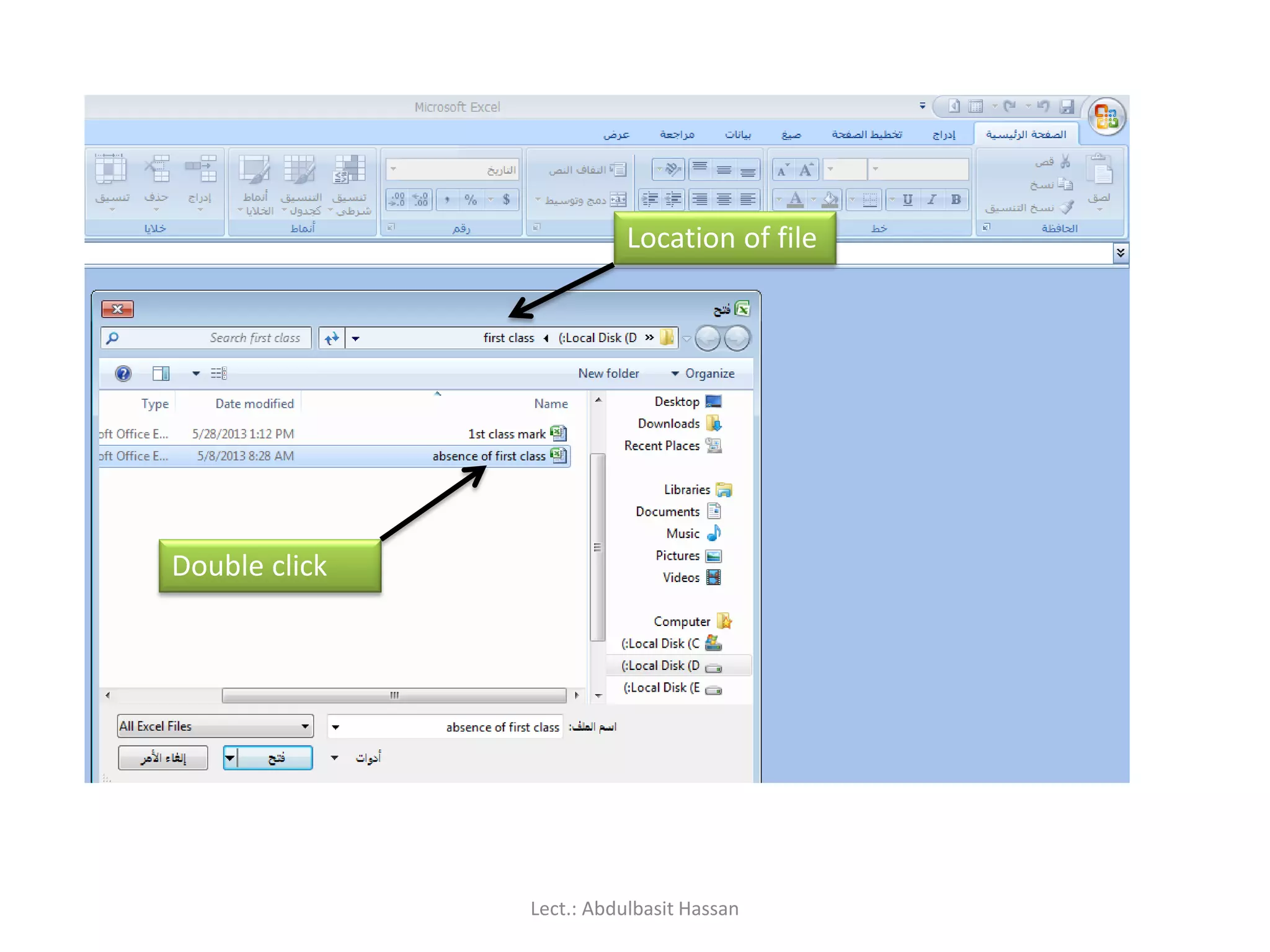
If youhave an icon on the desktop for Excel, then all you have to do
is double-click it to open Excel.
Double click
Lect. : Abdulbasit Hassan
4.
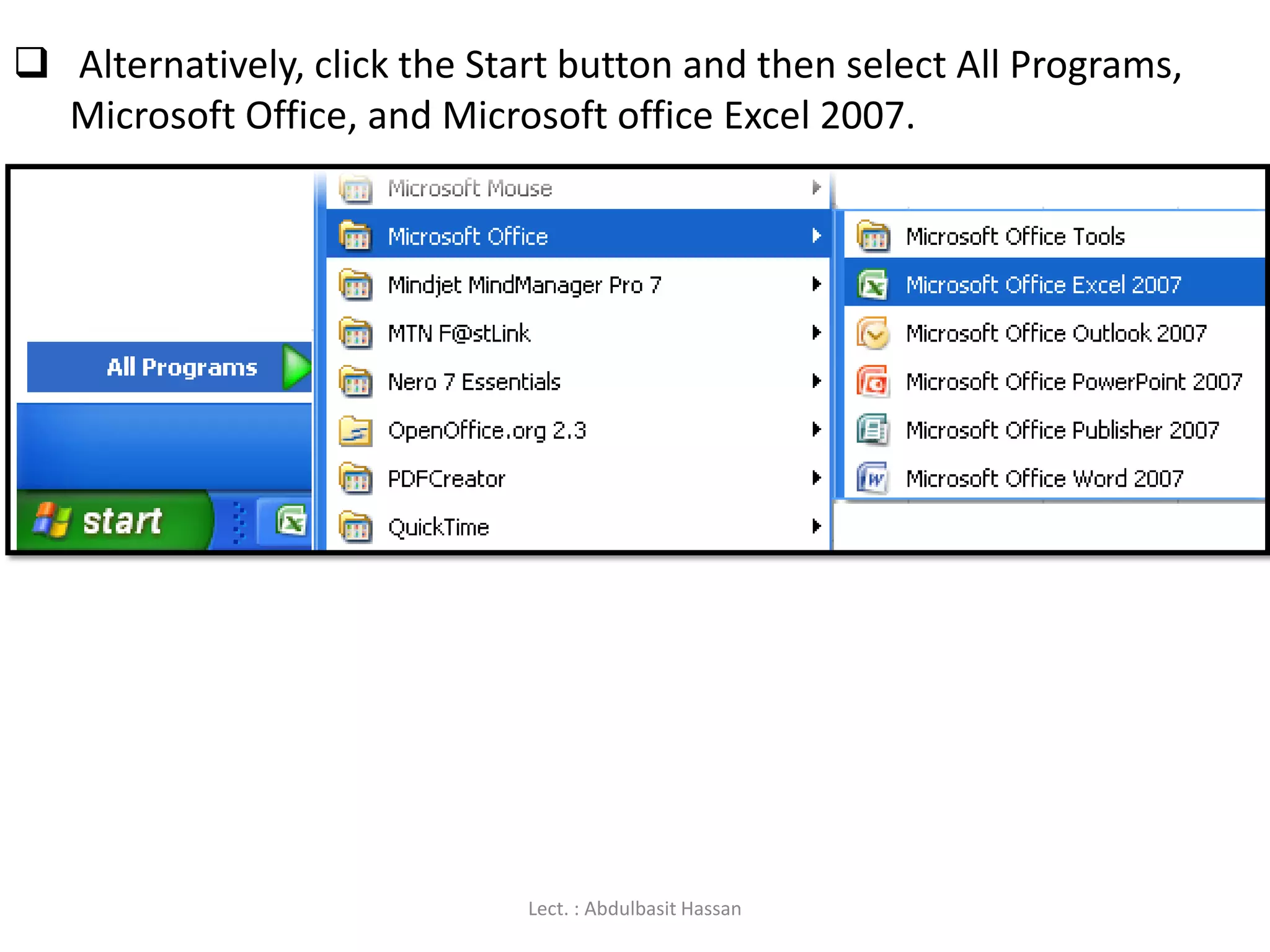
Alternatively, clickthe Start button and then select All Programs,
Microsoft Office, and Microsoft office Excel 2007.
Lect. : Abdulbasit Hassan
5.
Excel andWord have a lot in common, since it’s belong to the MS
Office group of programs.
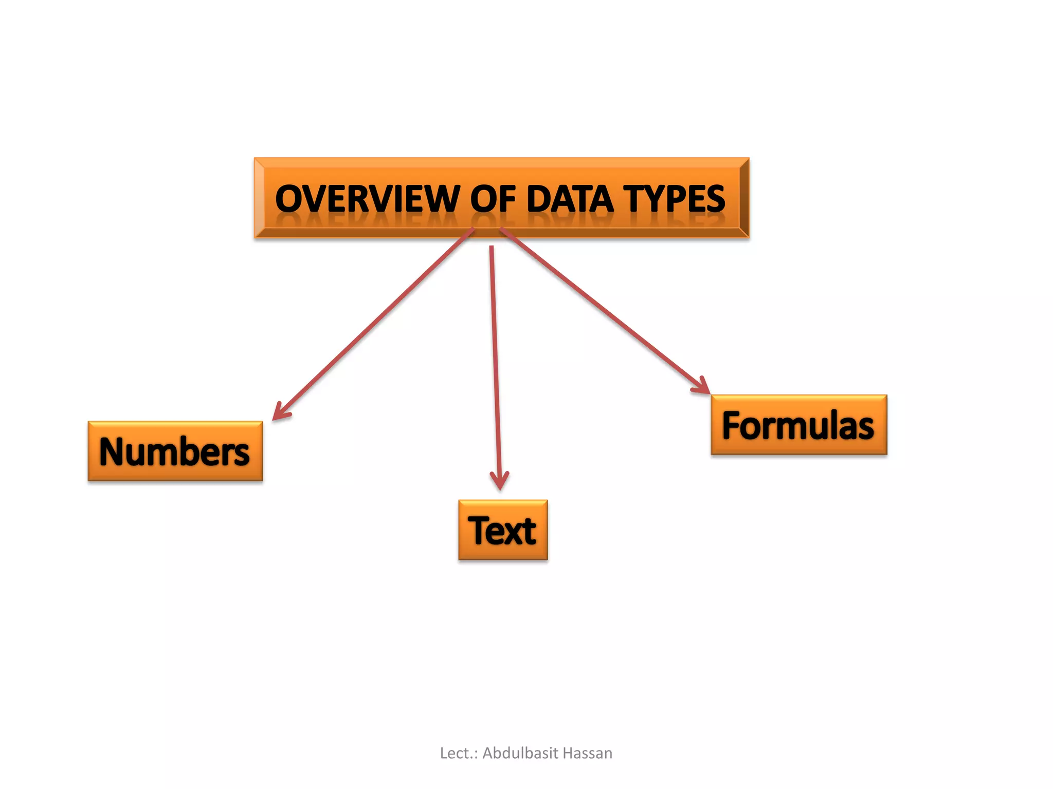
Excel is all about numbers. There’s almost no limit to what you can
do with numbers in Excel, including sorting, advanced calculations,
and graphing.
In addition, Excel’s formatting options mean that whatever you do
with your numbers, the result will always look professional!
Lect. : Abdulbasit Hassan
6.
Data filescreated with Excel are called workbooks (in the same way
as Word files are called documents).
This gives you the flexibility to store related data in different
locations within the same file.
More worksheets can be added, and others deleted, as required.
Each new workbook contains three separate
pages called worksheets (Sheet1, Sheet2, Sheet3).
Lect. : Abdulbasit Hassan
You’ll oftenhear Excel files referred to as spreadsheets. This is
a generic term, which sometimes means a workbook (file)
and sometimes means a worksheet (a page within the file).
For the sake of clarity, I’ll be using the terms
workbook and worksheet in this manual.
Lect. : Abdulbasit Hassan
9.
The Excel 2007window
As in Word 2007, the old menu system has been
replaced by the Ribbon and the Office button.
Lect. : Abdulbasit Hassan
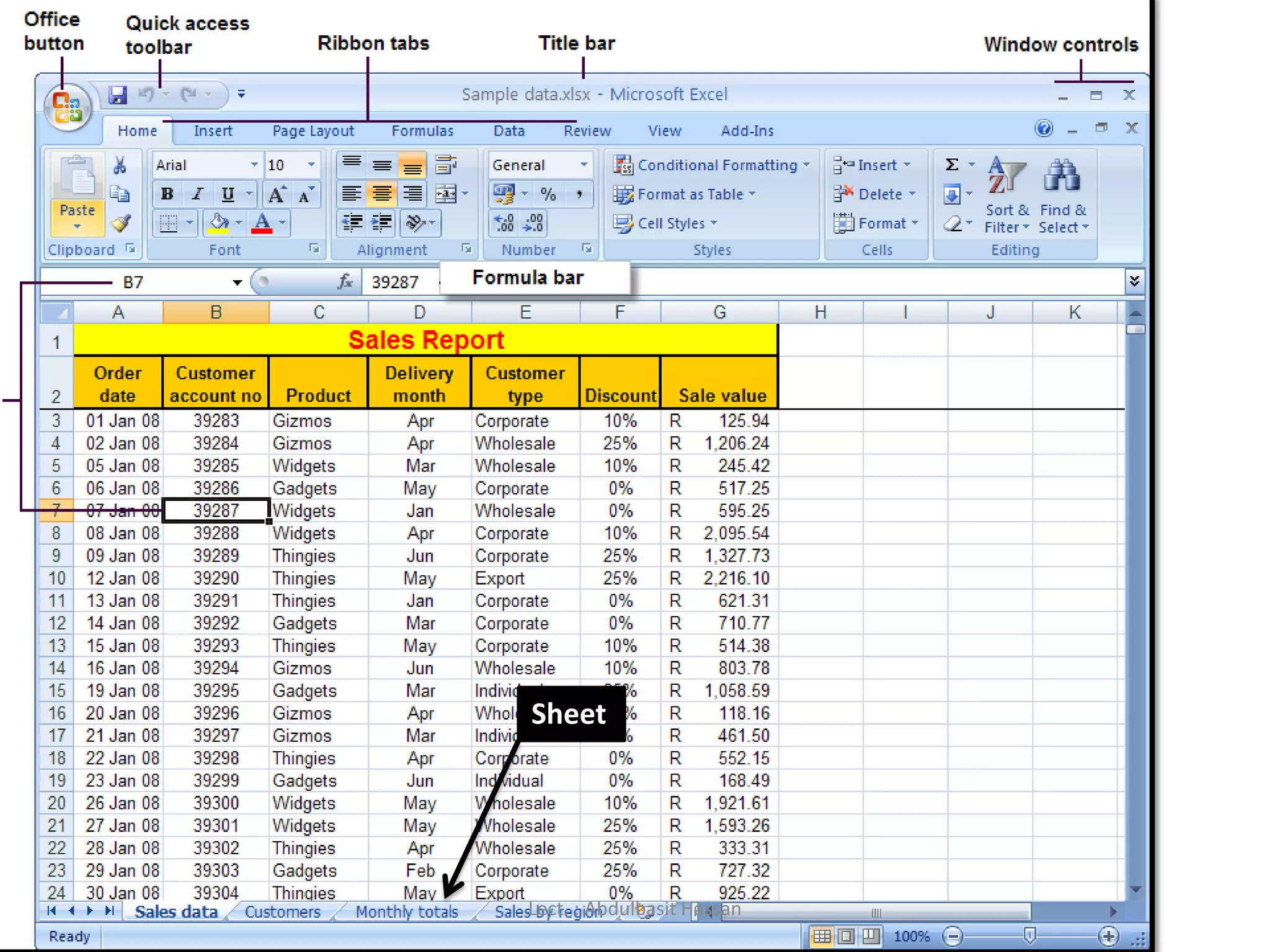
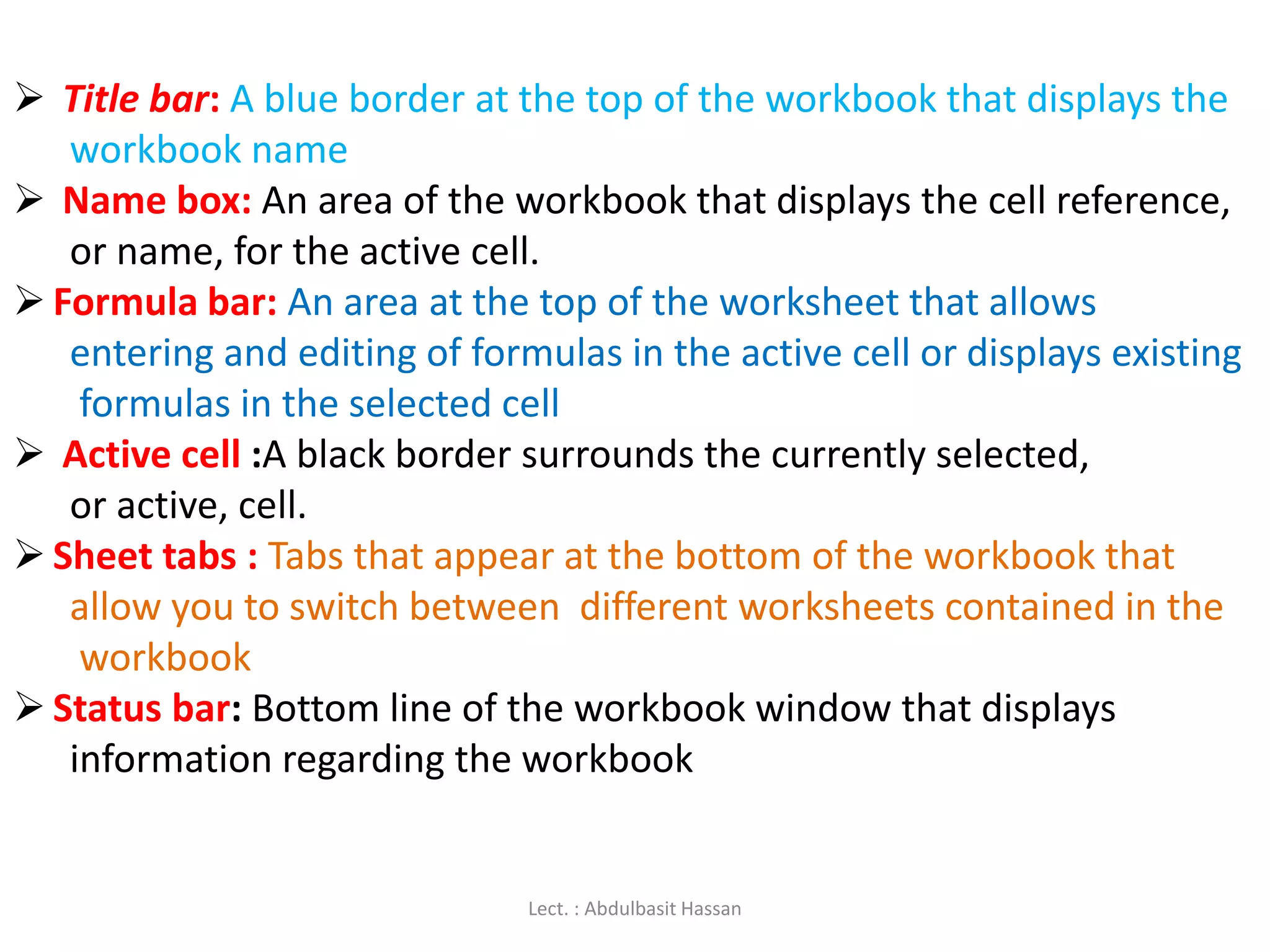
Title bar:A blue border at the top of the workbook that displays the
workbook name
Name box: An area of the workbook that displays the cell reference,
or name, for the active cell.
Formula bar: An area at the top of the worksheet that allows
entering and editing of formulas in the active cell or displays existing
formulas in the selected cell
Active cell :A black border surrounds the currently selected,
or active, cell.
Sheet tabs : Tabs that appear at the bottom of the workbook that
allow you to switch between different worksheets contained in the
workbook
Status bar: Bottom line of the workbook window that displays
information regarding the workbook
Lect. : Abdulbasit Hassan
12.
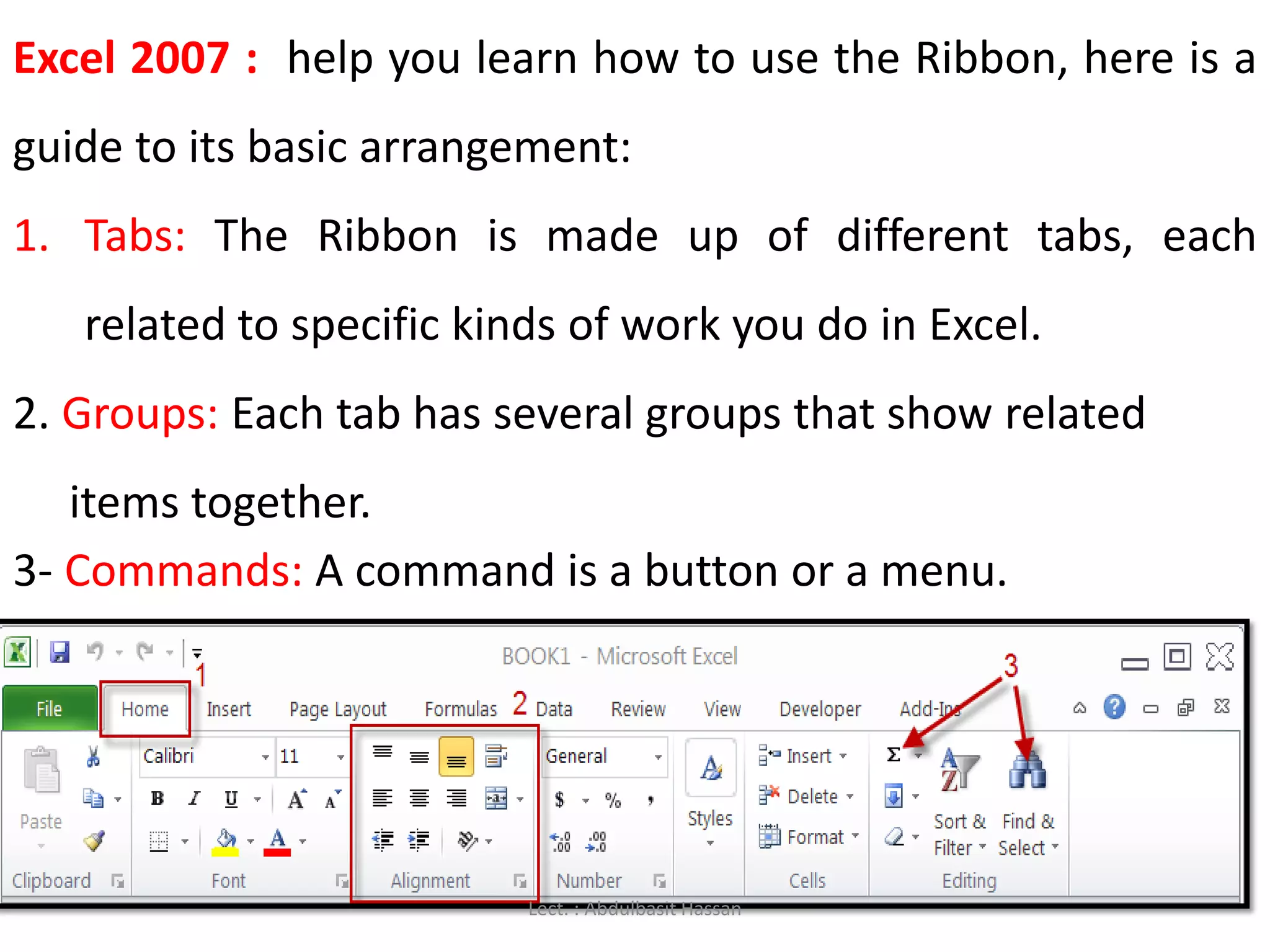
Excel 2007 :help you learn how to use the Ribbon, here is a
guide to its basic arrangement:
1. Tabs: The Ribbon is made up of different tabs, each
related to specific kinds of work you do in Excel.
2. Groups: Each tab has several groups that show related
items together.
3- Commands: A command is a button or a menu.
Lect. : Abdulbasit Hassan
13.
The Ribbon
The ribbonis the panel at the top portion of the document.
It has seven tabs:
The groups are logical collections of features designed to perform
function that you will utilize in developing or editing your Excel
spreadsheets. Commonly utilized features are displayed on the Ribbon.
Lect. : Abdulbasit Hassan
14.
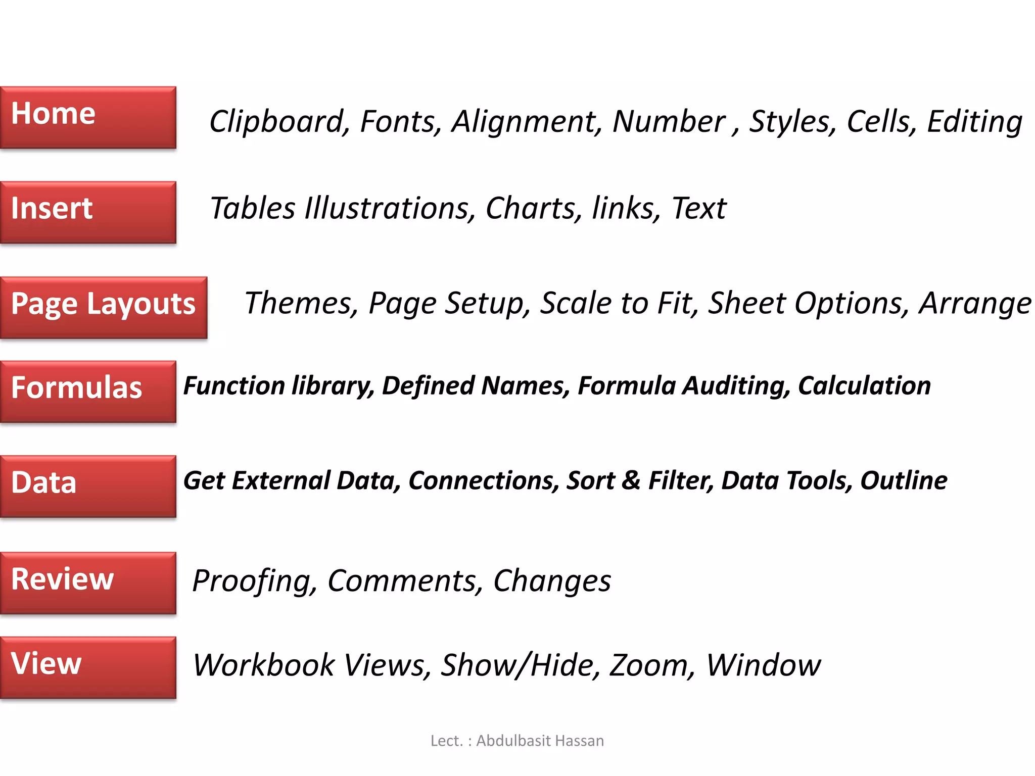
Home
Insert
Page Layouts
Formulas
Data
Review
View
Clipboard, Fonts,Alignment, Number , Styles, Cells, Editing
Tables Illustrations, Charts, links, Text
Themes, Page Setup, Scale to Fit, Sheet Options, Arrange
Function library, Defined Names, Formula Auditing, Calculation
Get External Data, Connections, Sort & Filter, Data Tools, Outline
Proofing, Comments, Changes
Workbook Views, Show/Hide, Zoom, Window
Lect. : Abdulbasit Hassan
15.
Notice:
The workingarea of the screen is divided into rows (1, 2, 3, 4, ...)
and columns (A, B, C, D, …).
Together these provide an address, such a C10 or G21, that uniquely
identifies each cell in the worksheet.
A range of cells extends in a rectangle from one cell to another,
and is referred to by using the first and last cell addresses separated
by a colon.
For example, the group of cells from A3 to G4 would be written as
A3:G4.
Lect. : Abdulbasit Hassan
16.
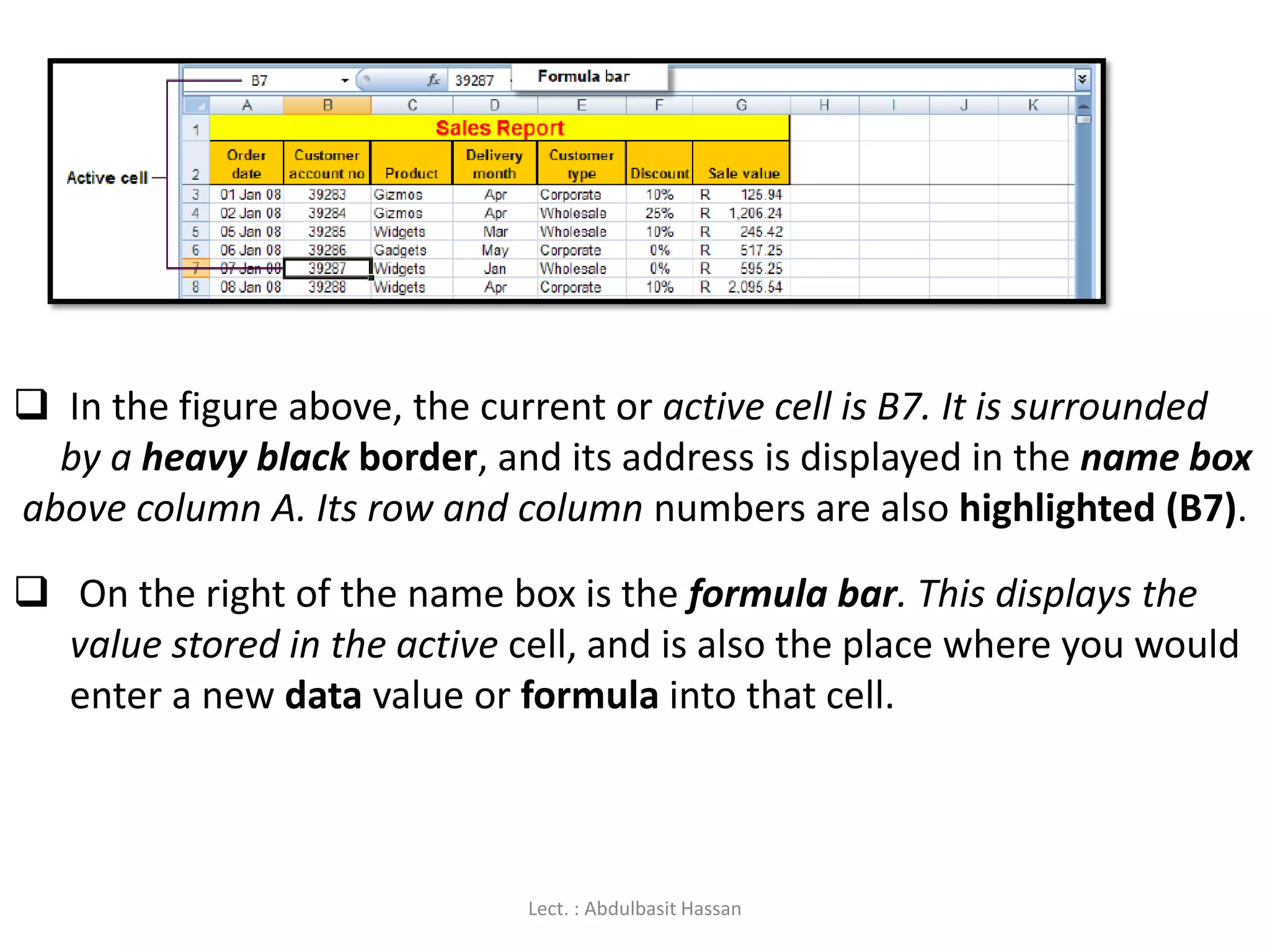
In thefigure above, the current or active cell is B7. It is surrounded
by a heavy black border, and its address is displayed in the name box
above column A. Its row and column numbers are also highlighted (B7).
On the right of the name box is the formula bar. This displays the
value stored in the active cell, and is also the place where you would
enter a new data value or formula into that cell.
Lect. : Abdulbasit Hassan
17.
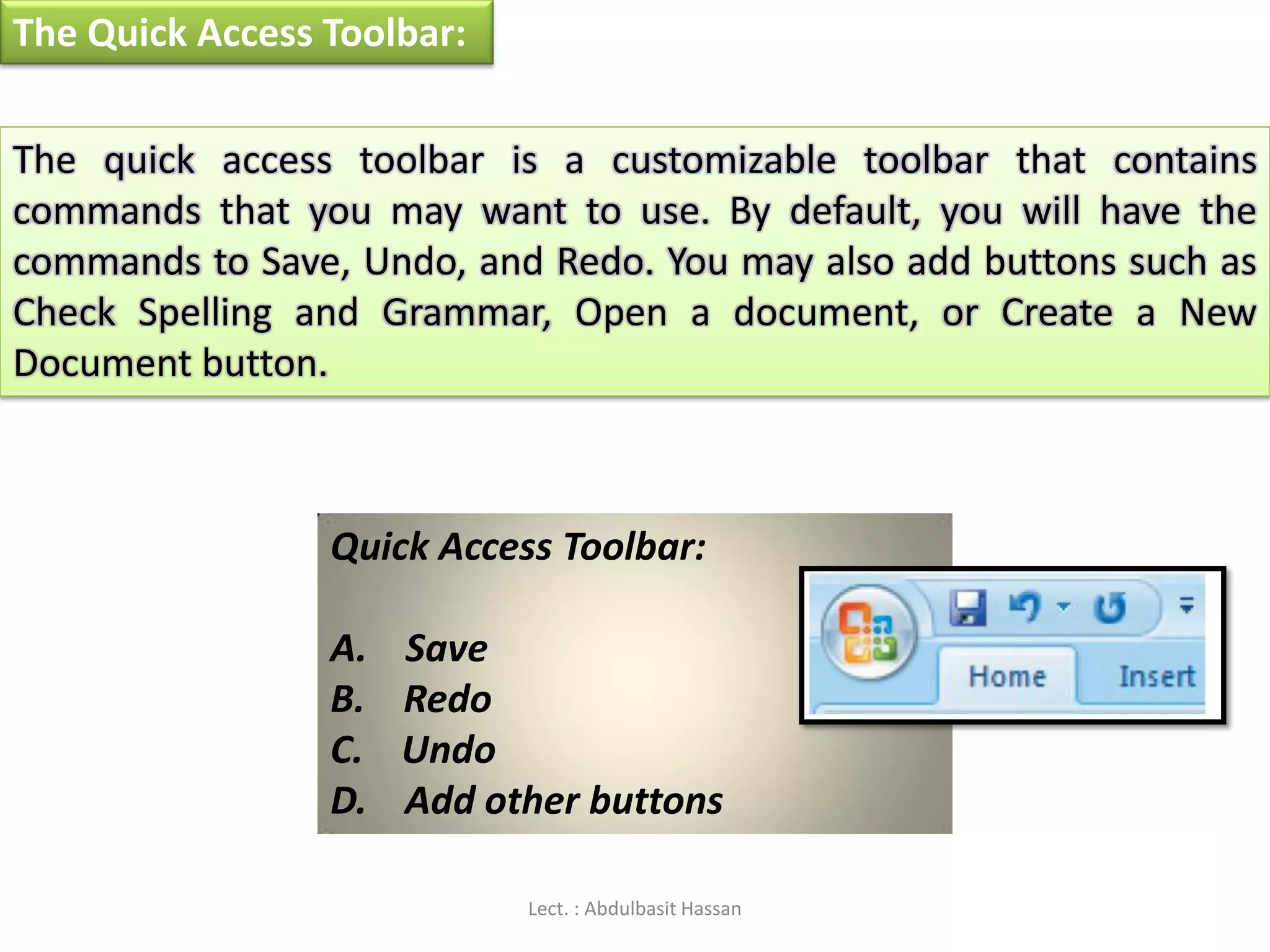
The Quick AccessToolbar:
The quick access toolbar is a customizable toolbar that contains
commands that you may want to use. By default, you will have the
commands to Save, Undo, and Redo. You may also add buttons such as
Check Spelling and Grammar, Open a document, or Create a New
Document button.
Quick Access Toolbar:
A. Save
B. Redo
C. Undo
D. Add other buttons
Lect. : Abdulbasit Hassan
18.
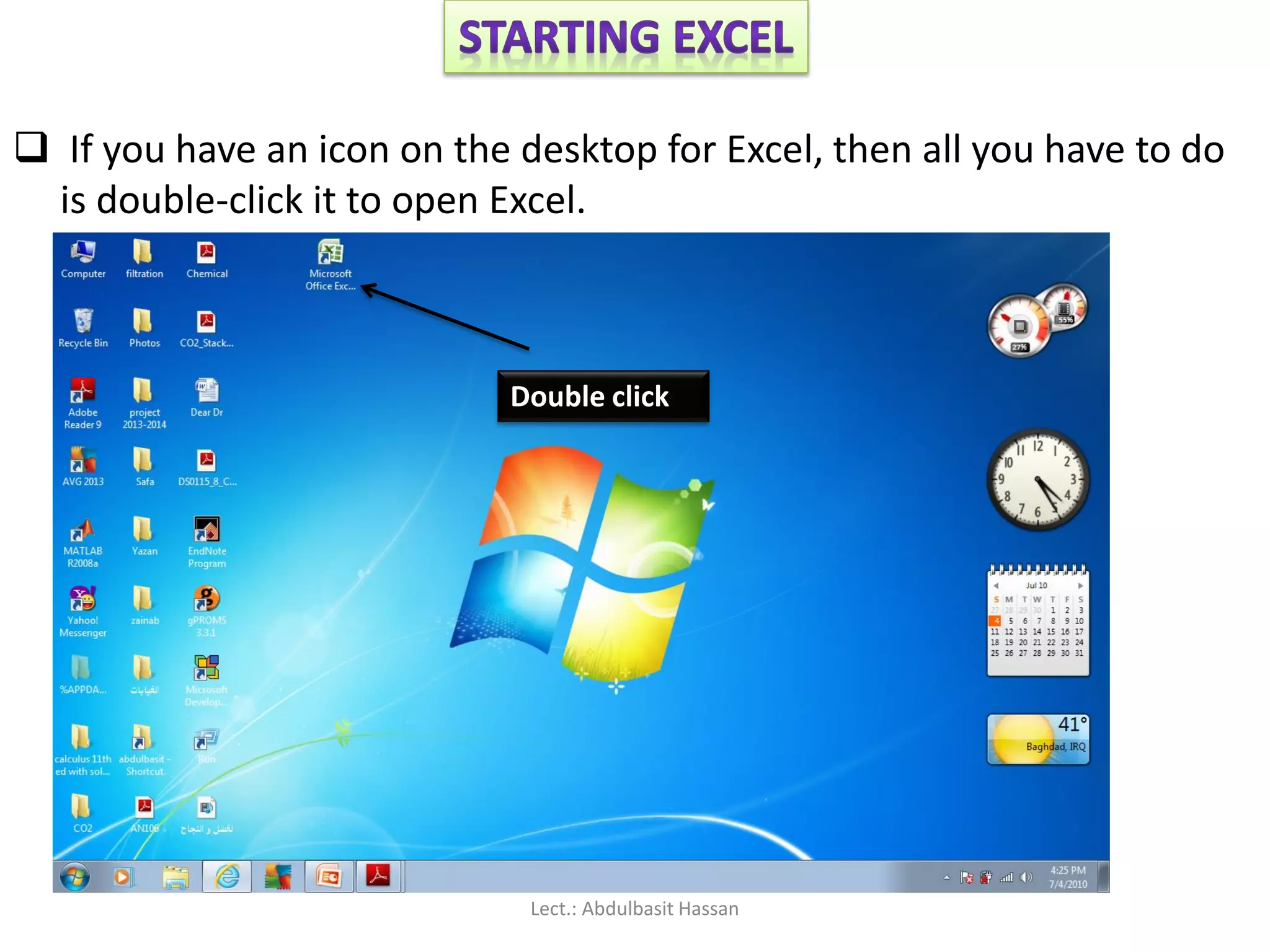
If youhave an icon on the desktop for Excel, then all you have to do
is double-click it to open Excel.
Double click
Lect.: Abdulbasit Hassan
19.
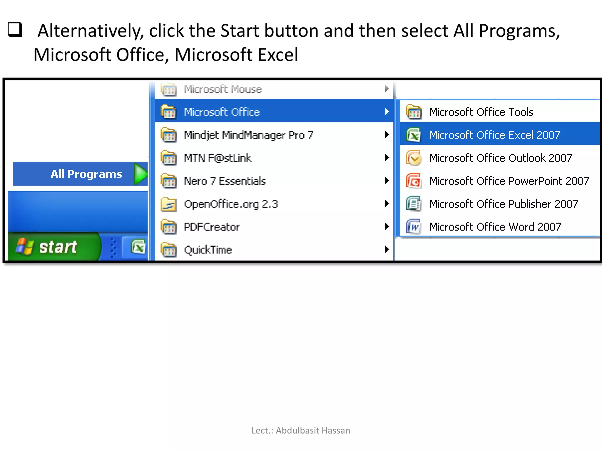
Alternatively, clickthe Start button and then select All Programs,
Microsoft Office, Microsoft Excel
Lect.: Abdulbasit Hassan
20.
When youopen Excel from a desktop icon or from the Start menu, a
new empty workbook (consisting of three worksheets) will be
displayed on your screen.
If you double-click on an existing Excel file from inside the Windows
Explorer window, then Excel will open and display the selected file on
your screen.
Lect.: Abdulbasit Hassan
21.
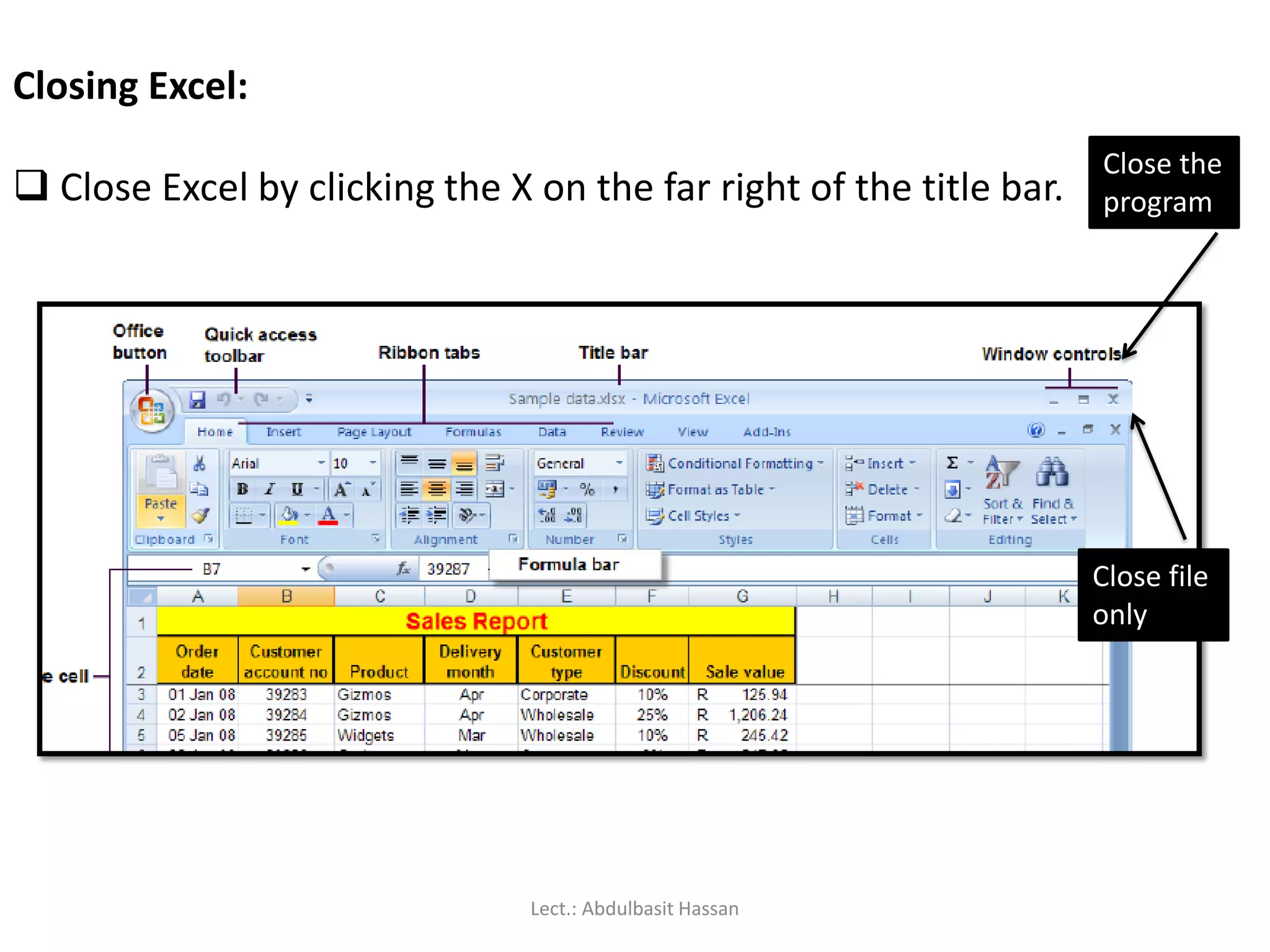
Closing Excel:
CloseExcel by clicking the X on the far right of the title bar.
Close file
only
Close the
program
Lect.: Abdulbasit Hassan
22.
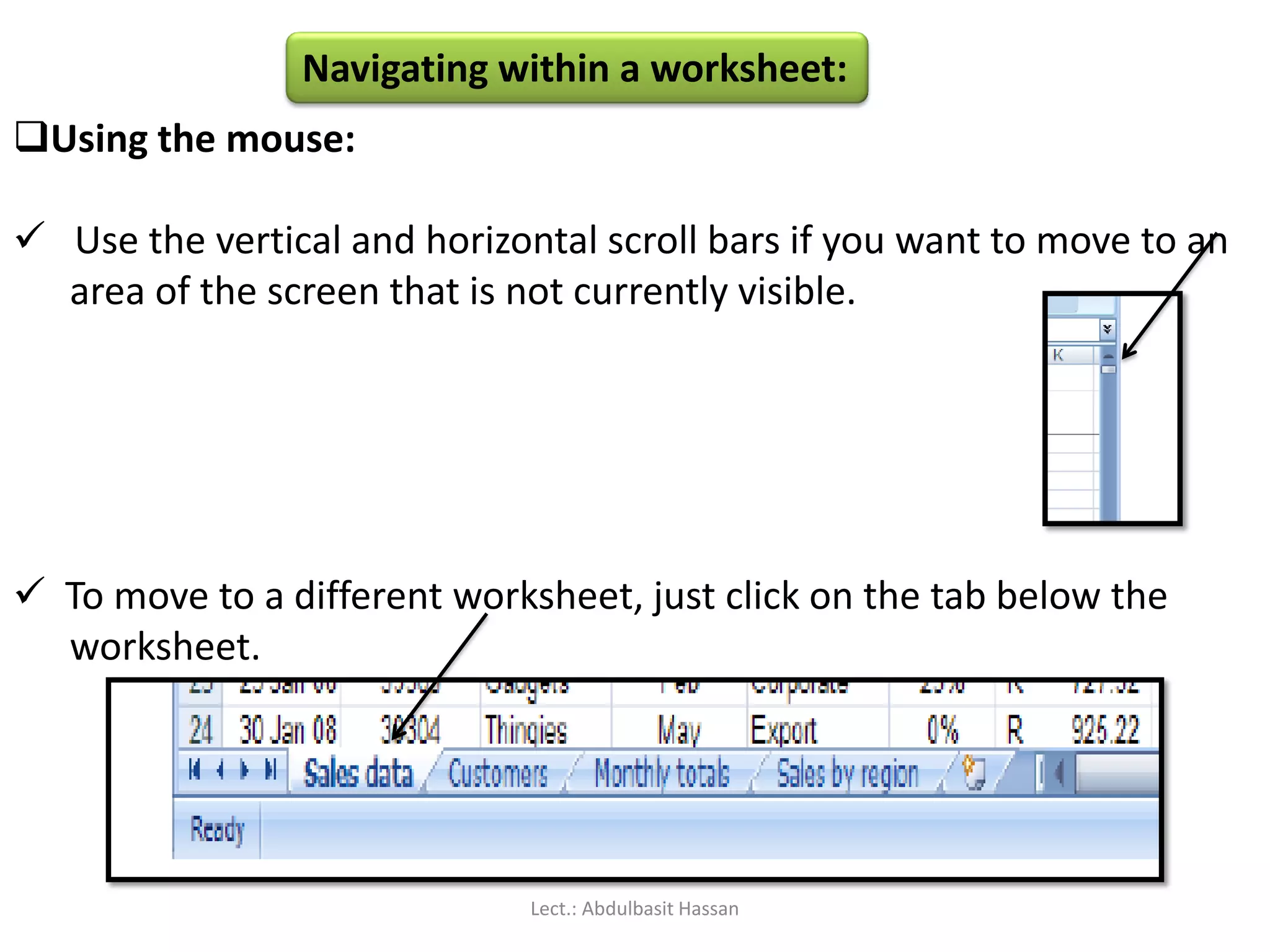
Navigating within aworksheet:
Using the mouse:
Use the vertical and horizontal scroll bars if you want to move to an
area of the screen that is not currently visible.
To move to a different worksheet, just click on the tab below the
worksheet.
Lect.: Abdulbasit Hassan
23.
Using the keyboard:
Use the arrow keys, or [PAGE UP] and [PAGE DOWN], to move to
a different area of the screen.
[CTRL] + [HOME} will take you to cell A1.
[CTRL] + [PAGE DOWN] will take you to the next worksheet,
[CTRL] + [PAGE UP] for the preceding worksheet.
PAGE UP
PAGE DOWN
CTRL
arrow
HOME
You can jump quickly to a specific cell by pressing [F5] and typing
in the cell address.
You can also type the cell address in the name box above column A,
and press [ENTER].
Lect.: Abdulbasit Hassan
24.
Selecting cells:
Using themouse:
Click on a cell to select it.
You can select a range of adjacent cells by clicking on the first one,
and then dragging the mouse over the others.
You can select a set of non-adjacent cells by clicking on the first one,
and then holding down the [CTRL] key as you click on the others.
Lect.: Abdulbasit Hassan
25.
Using the keyboard:
Use the arrow keys to move to the desired cell, which is
automatically selected.
To select multiple cells, hold down the [SHIFT] key while the
first cell is active, and then use the arrow keys to select the
rest of the range.
Lect.: Abdulbasit Hassan
26.
Selecting rows orcolumns:
To select all the cells in a particular row, just click on the row
number (1, 2, 3, etc) at the left edge of the worksheet.
Hold down the mouse button and drag across row numbers to
select multiple adjacent rows.
Hold down [CTRL] if you want to select a set of non-adjacent rows.
Lect.: Abdulbasit Hassan
27.
Similarly, toselect all the cells in column, you should click on the
column heading (A, B, C, etc) at the top edge of the worksheet.
Hold down the mouse button and drag across column headings to
select multiple adjacent columns.
Hold down [CTRL] if you want to select a set of non-adjacent columns.
Lect.: Abdulbasit Hassan
28.
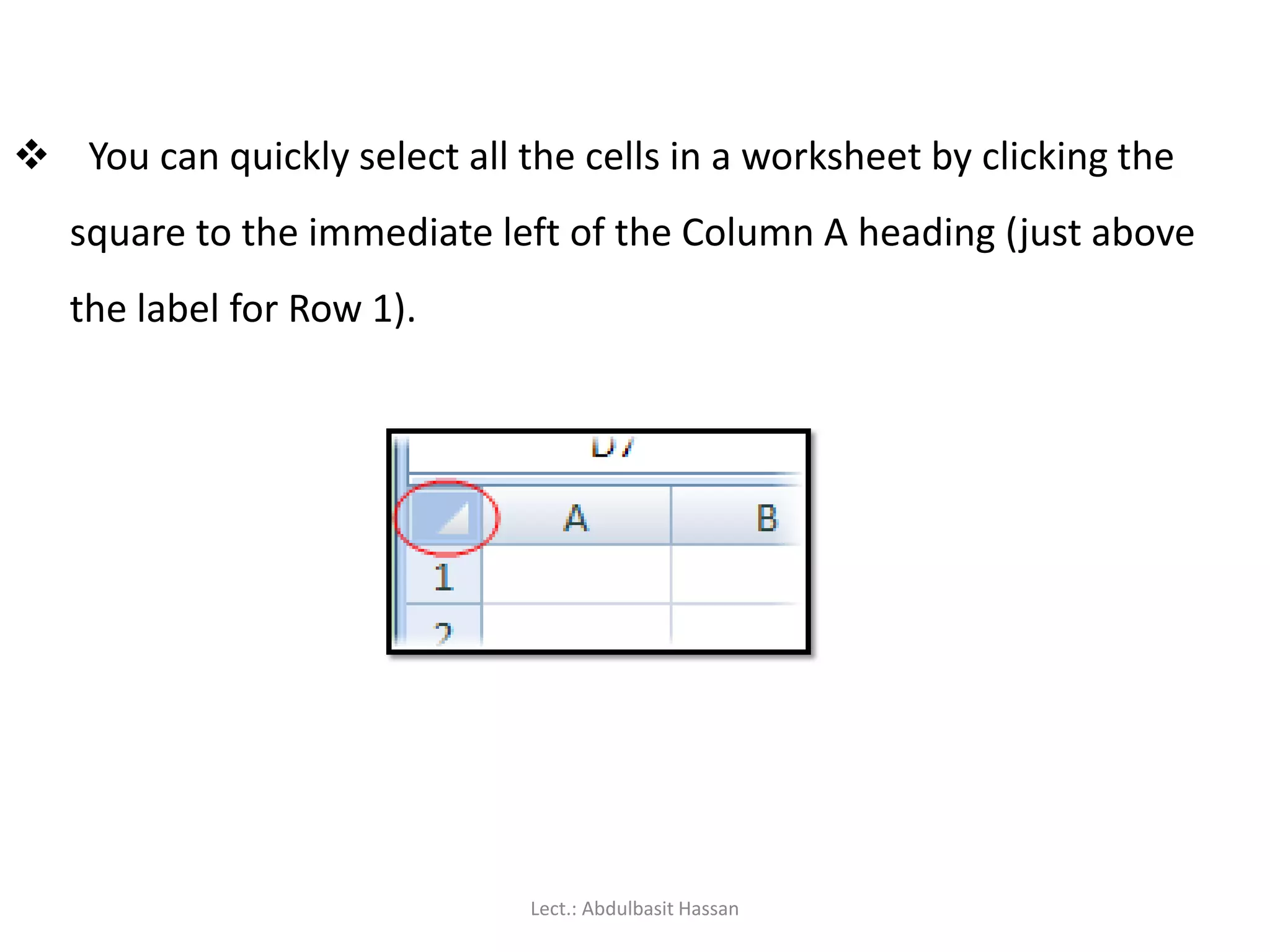
You canquickly select all the cells in a worksheet by clicking the
square to the immediate left of the Column A heading (just above
the label for Row 1).
Lect.: Abdulbasit Hassan
First you needa workbook:
Before you start entering data, you need to decide whether this is a
completely new project deserving a workbook of its own, or whether
the data you are going to enter relates to an existing workbook.
Remember that you can always add a new worksheet to an existing
workbook, and you’ll find it much easier to work with related data if it’s
all stored in the same file.
Lect.: Abdulbasit Hassan
31.
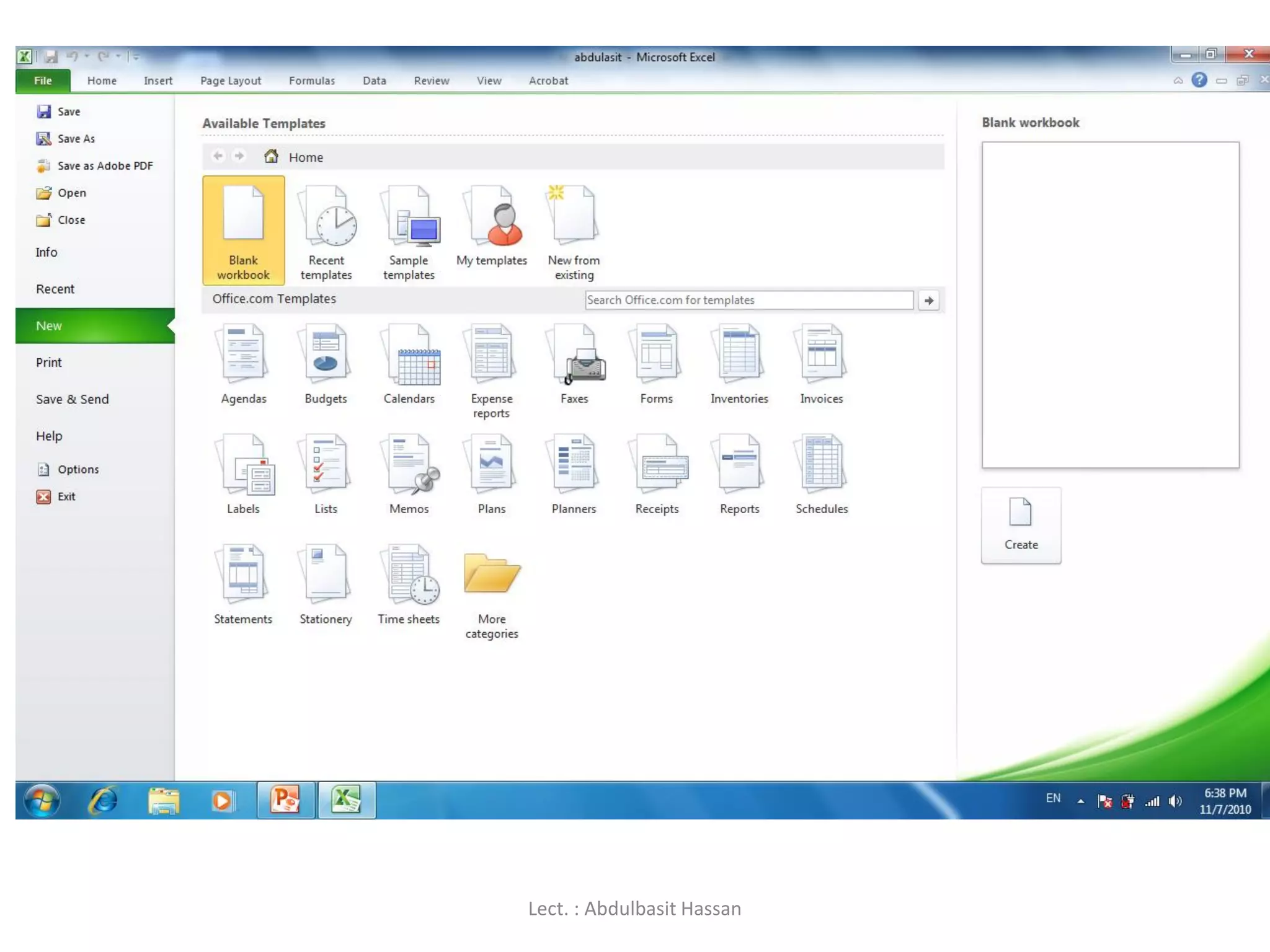
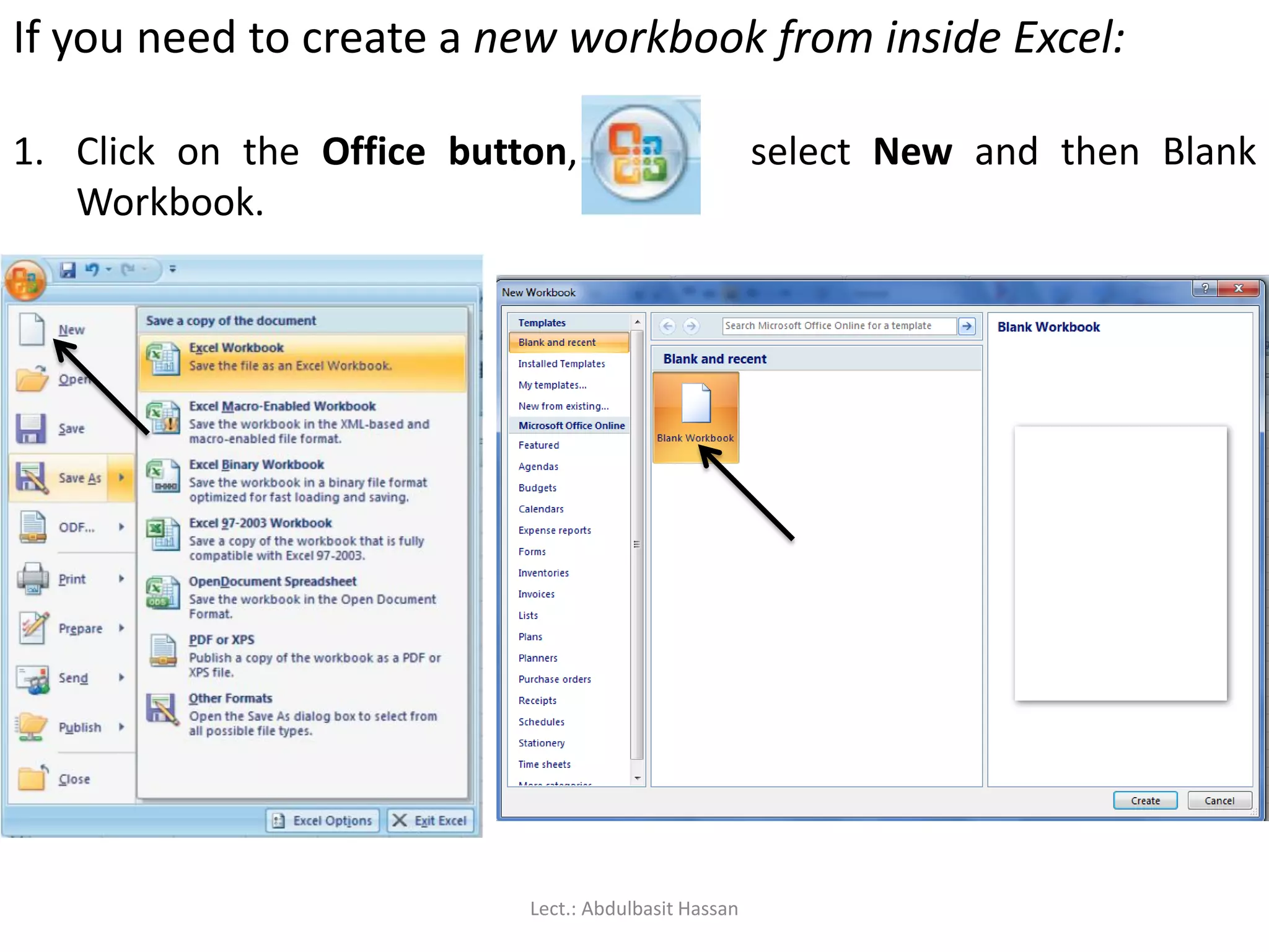
If you needto create a new workbook from inside Excel:
1. Click on the Office button, select New and then Blank
Workbook.
Lect.: Abdulbasit Hassan
32.
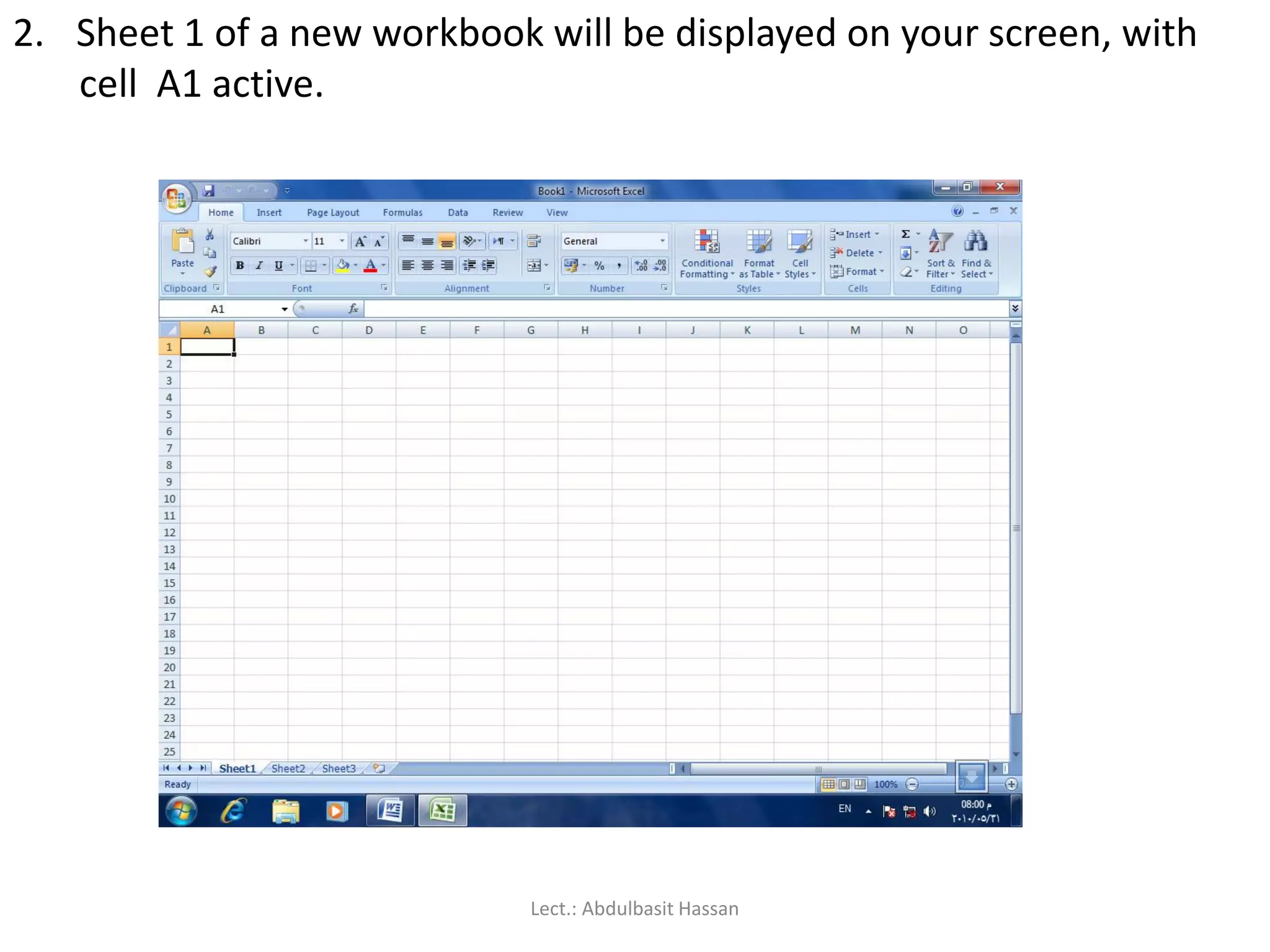
2. Sheet 1of a new workbook will be displayed on your screen, with
cell A1 active.
Lect.: Abdulbasit Hassan
33.
To open anexisting workbook from inside Excel:
1. Click on the Office button, click Open, and then navigate to
the drive and folder containing the file you want to open.
Lect.: Abdulbasit Hassan
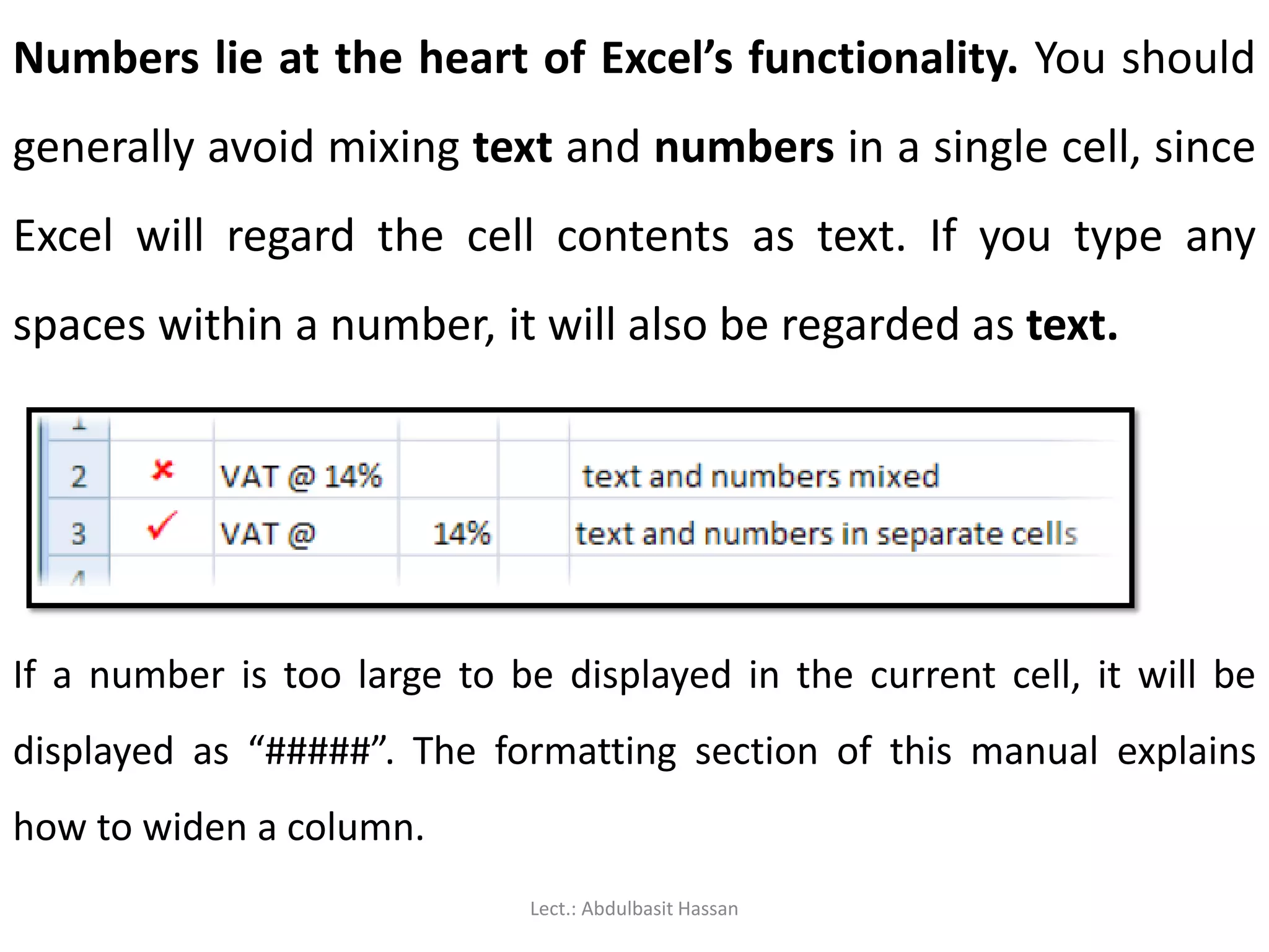
Numbers lie atthe heart of Excel’s functionality. You should
generally avoid mixing text and numbers in a single cell, since
Excel will regard the cell contents as text. If you type any
spaces within a number, it will also be regarded as text.
If a number is too large to be displayed in the current cell, it will be
displayed as “#####”. The formatting section of this manual explains
how to widen a column.
Lect.: Abdulbasit Hassan
38.
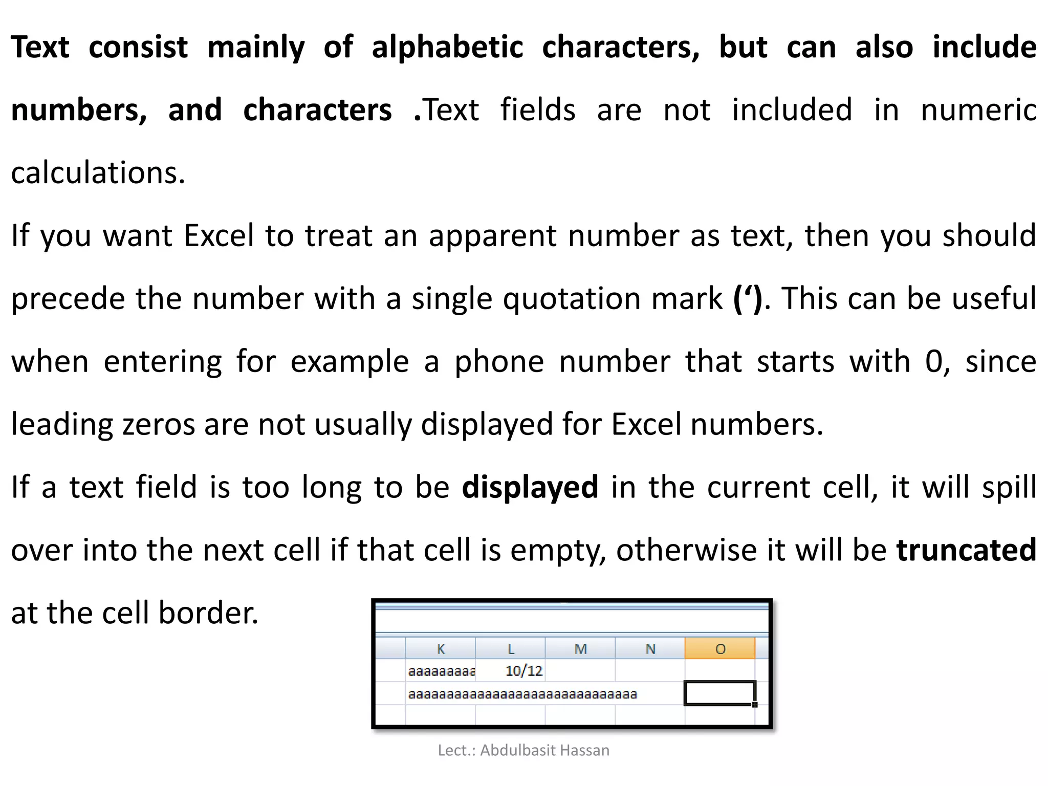
Text consist mainlyof alphabetic characters, but can also include
numbers, and characters .Text fields are not included in numeric
calculations.
If you want Excel to treat an apparent number as text, then you should
precede the number with a single quotation mark (‘). This can be useful
when entering for example a phone number that starts with 0, since
leading zeros are not usually displayed for Excel numbers.
If a text field is too long to be displayed in the current cell, it will spill
over into the next cell if that cell is empty, otherwise it will be truncated
at the cell border.
Lect.: Abdulbasit Hassan
39.
Formulas are themost powerful elements of an Excel spreadsheet.
Every formula starts with an “=” sign, and contains at least one logical or
mathematical operation (or special function), combined with numbers
and/or cell references. We’ll discuss formulas and functions in more
detail later in the manual.
Lect.: Abdulbasit Hassan
40.
Data entry cellby cell
To enter either numbers or text:
1. Click on the cell where you want the data to be stored, so that the
cell becomes active.
2. Type the number or text.
3. Press [ENTER] to move to the next row, or [TAB] to move to the next
column. Until
4- you’ve pressed [ENTER] or [TAB], you can cancel the data entry by
pressing [ESC].
5- To enter a date, use a slash or hyphen between the day, month and
year, for example 14/02/2009. Use a colon between hours, minutes
and seconds, for example 13:45:20.
Lect.: Abdulbasit Hassan
41.
Deleting data:
You wantto delete data that’s already been entered in a
worksheet? Simple!
1. Select the cell or cells containing data to be deleted.
2. Press the [DEL] key on your keyboard.
3. The cells remain in the same position as before, but their
contents are deleted.
Lect.: Abdulbasit Hassan
42.
Moving data :
You’vealready entered some data, and want to move it to a different
area on the worksheet?
1. Select the cells you want to move (they will become highlighted).
2. Move the cursor to the border of the highlighted cells. When the
cursor changes from a white cross to a four-headed arrow (the move
pointer), hold down the left mouse button.
3. Drag the selected cells to a new area of the worksheet, then release
the mouse button.
4. You can also cut the selected data using the ribbon icon or [CTRL] +
[X], then click in the top left cell of the destination area and paste the
data with the ribbon icon or [CTRL] + [V].
Lect.: Abdulbasit Hassan
Copying data:
To copyexisting cell contents to another area on the worksheet:
1. Select the cells you want to copy (they will become highlighted).
2. Move the cursor to the border of the highlighted cells while hold in
down the [CTRL] key. When the cursor changes from a white cross to
a hollow left-pointing arrow (the copy pointer), hold down the left
mouse button.
3. Drag the selected cells to a second area of the worksheet, then
release the mouse button.
4. You can also copy the selected data using the ribbon icon or [CTRL] +
[C], then click in the top left cell of the destination area and paste the
data with the ribbon icon or [CTRL] + [V].
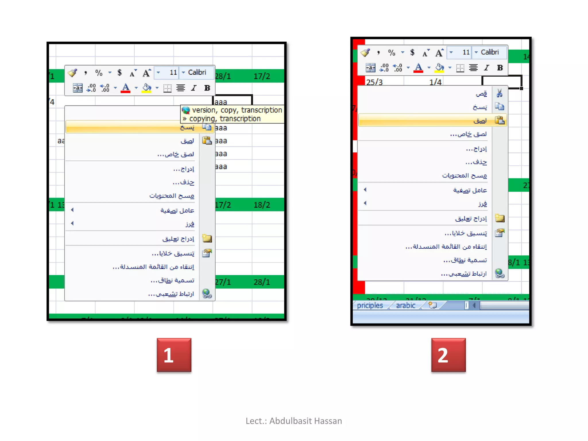
5. You can also copy the selected data by right click mouse , select copy
, and go to new cell also right click and select paste.
Lect.: Abdulbasit Hassan
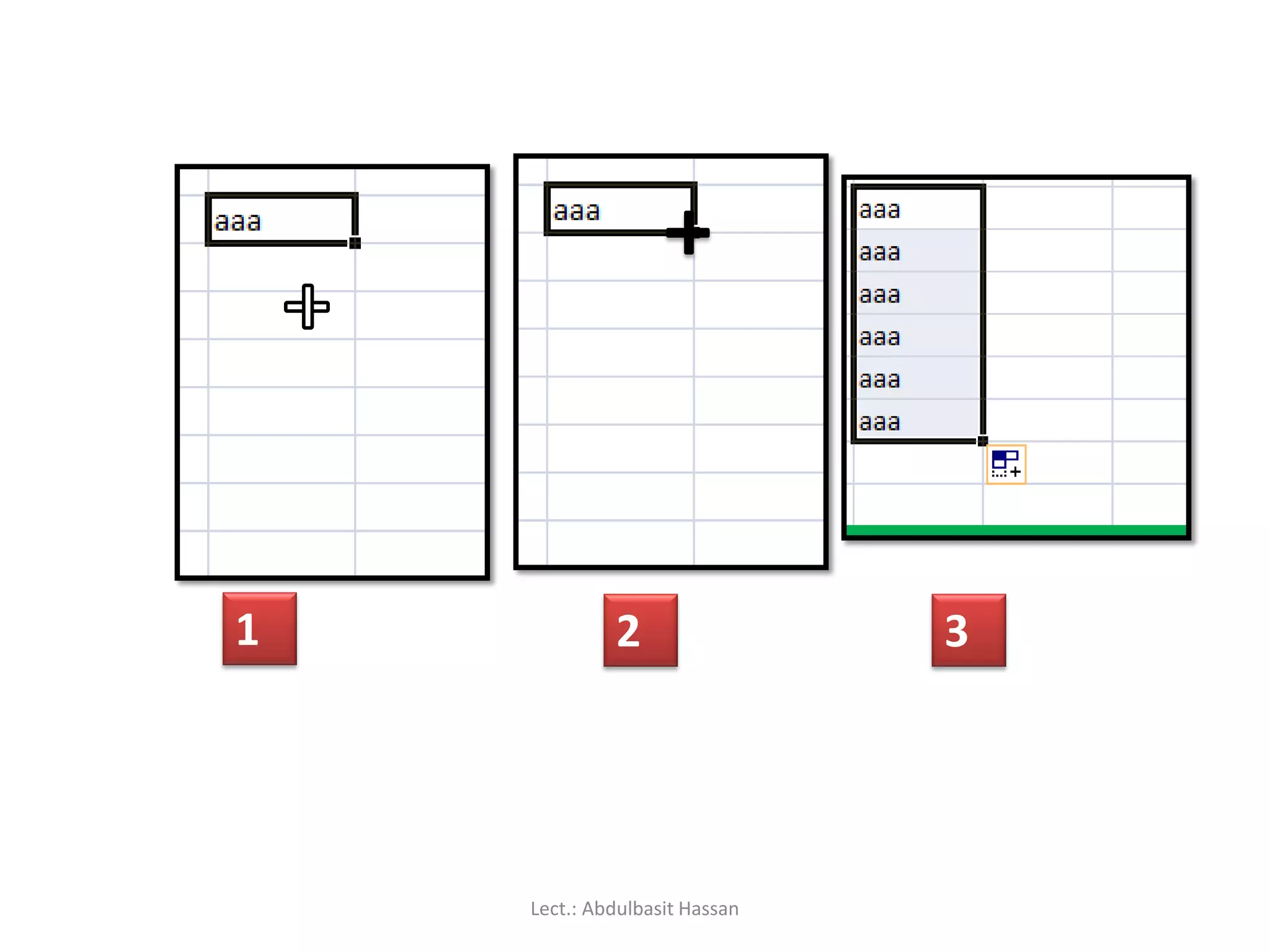
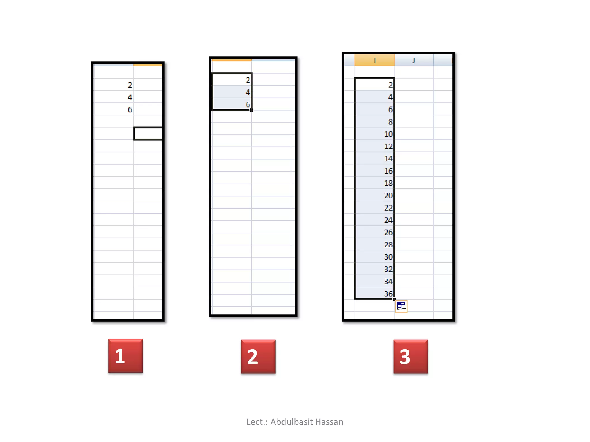
Using Auto fill:
Thisis one of Excel’s niftiest features! It takes no effort at all to repeat a
data series (such as the days of the week, months of the year, or a
numbers series such as odd numbers) over a range of cells.
1. Enter the start of the series into a few adjacent cells (enough to
show the underlying pattern).
2. Select the cells that contain series data.
3. Move the cursor over the small square in the bottom right-hand
corner of the selection (the fill handle). Hold down the mouse button
and drag to a range of adjacent cells.
4. The target cells will be filled based on the pattern of the original
series cells.
Lect.: Abdulbasit Hassan
In this section,we will learn how to save an Excel 2007
Document in Compatibility Mode. Compatibility Mode will
allow you to create spreadsheets in Excel 2007, and if you
use another computer with an older version of Excel, this
feature will allow you to open the spreadsheet and make
changes!
Lect.: Abdulbasit Hassan
51.
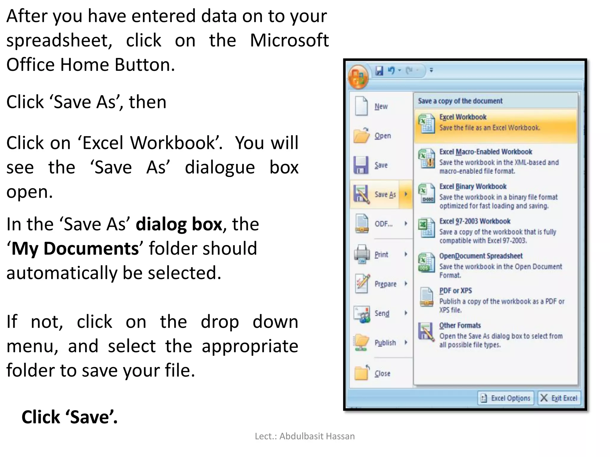
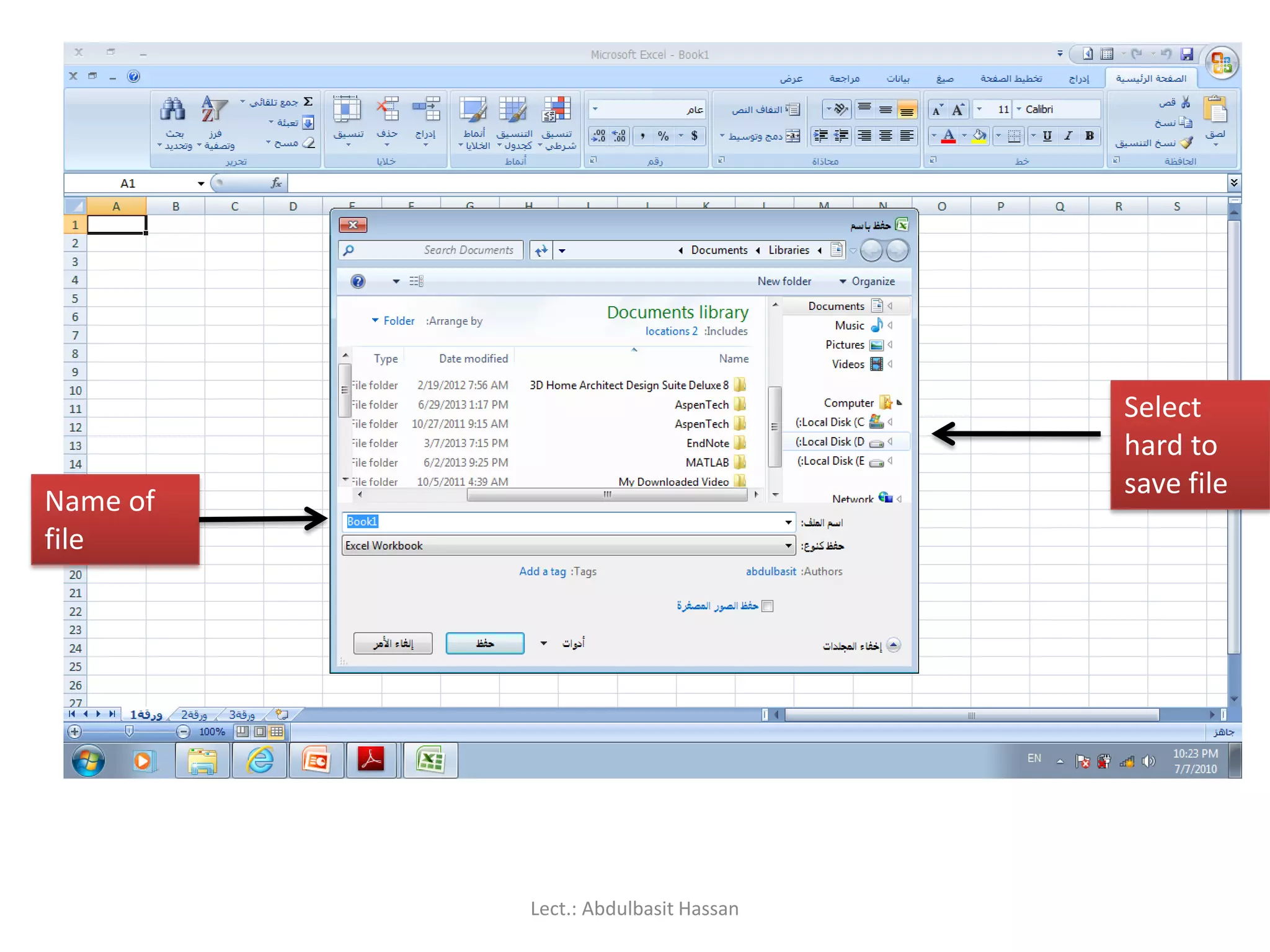
After you haveentered data on to your
spreadsheet, click on the Microsoft
Office Home Button.
Click ‘Save As’, then
Click on ‘Excel Workbook’. You will
see the ‘Save As’ dialogue box
open.
In the ‘Save As’ dialog box, the
‘My Documents’ folder should
automatically be selected.
If not, click on the drop down
menu, and select the appropriate
folder to save your file.
Click ‘Save’.
Lect.: Abdulbasit Hassan
Editing data
In dataentry mode, when you move the cursor to a
new cell, anything you type replaces the previous cell
contents. Edit mode allow you to amend existing cell
contents without having to retype the entire entry.
Note: that while you are in edit mode, many of the
Ribbon commands are disabled.
Lect.: Abdulbasit Hassan
Editing cell contents
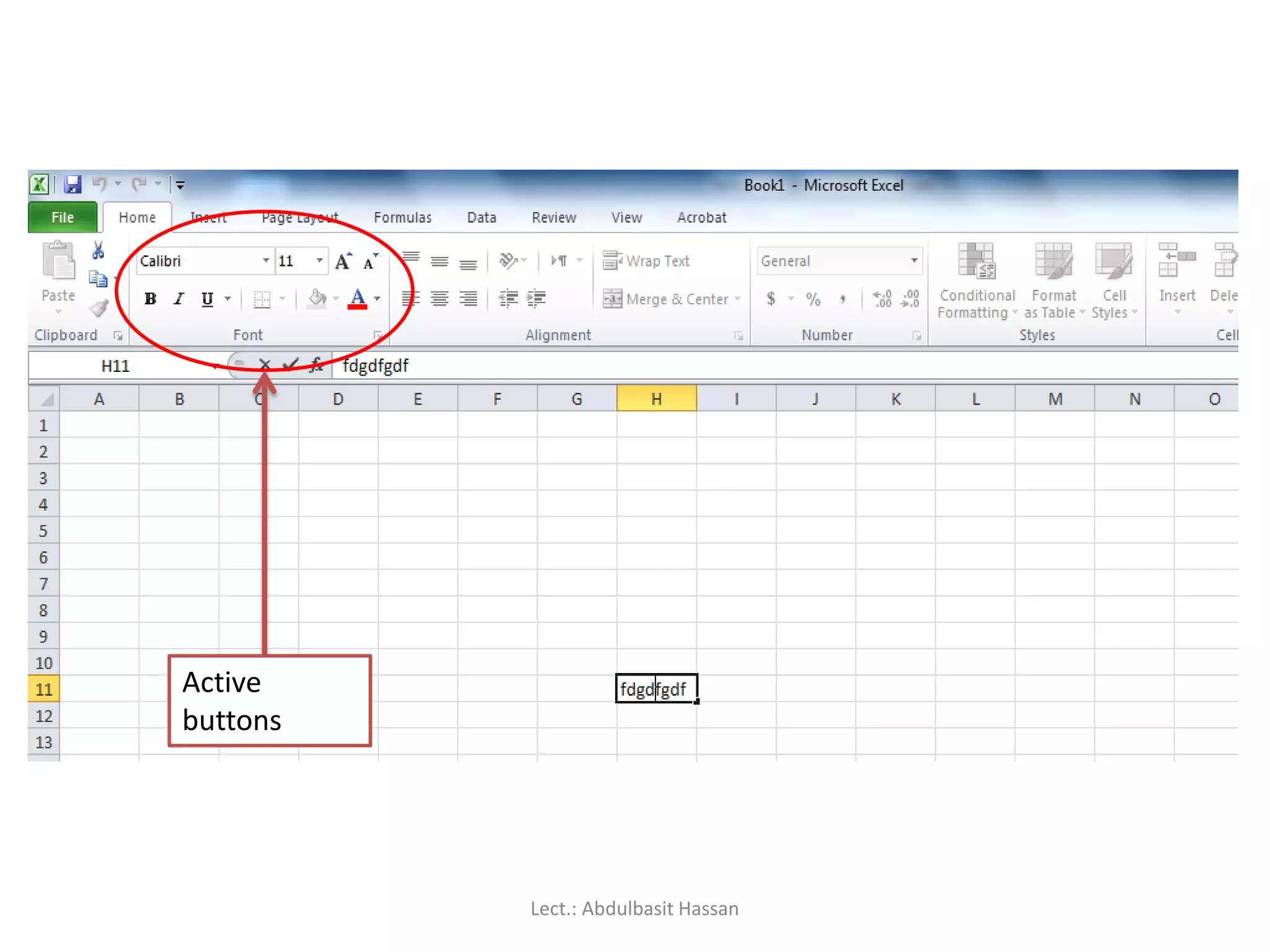
Thereare two different ways to enter edit mode: either double-click on
the cell whose contents you want to edit, or else click to select the cell
you want to edit, and then click anywhere in the formula bar.
To delete characters, use the [BACKSPACE] or [DEL] key.
To insert characters, click where you want to insert them, and then
type.
You can force a line break within the current cell contents by typing
[ALT] + [ENTER], or by Space key.
Exit edit mode by pressing [ENTER].
Lect.: Abdulbasit Hassan
56.
Common problems
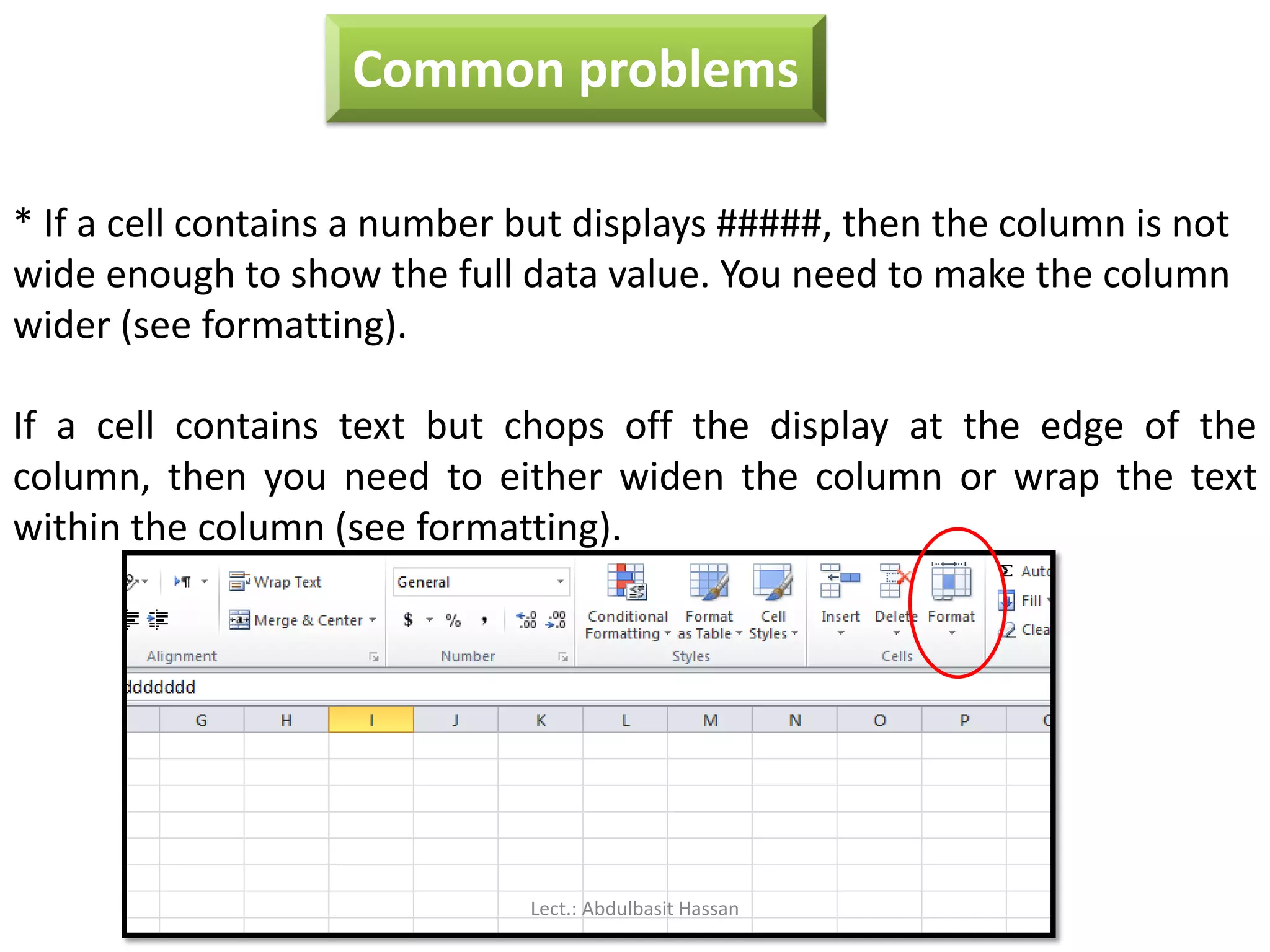
* Ifa cell contains a number but displays #####, then the column is not
wide enough to show the full data value. You need to make the column
wider (see formatting).
If a cell contains text but chops off the display at the edge of the
column, then you need to either widen the column or wrap the text
within the column (see formatting).
Lect.: Abdulbasit Hassan
57.
Inserting or deletingcells
You can insert a new cell above the current active cell, in
which case the active cell and those below it will each move
down one row.
You can also insert a new cell to the left of the current active
cell, in which case the active cell and those on its right will
each move one column to the right.
Lect.: Abdulbasit Hassan
58.
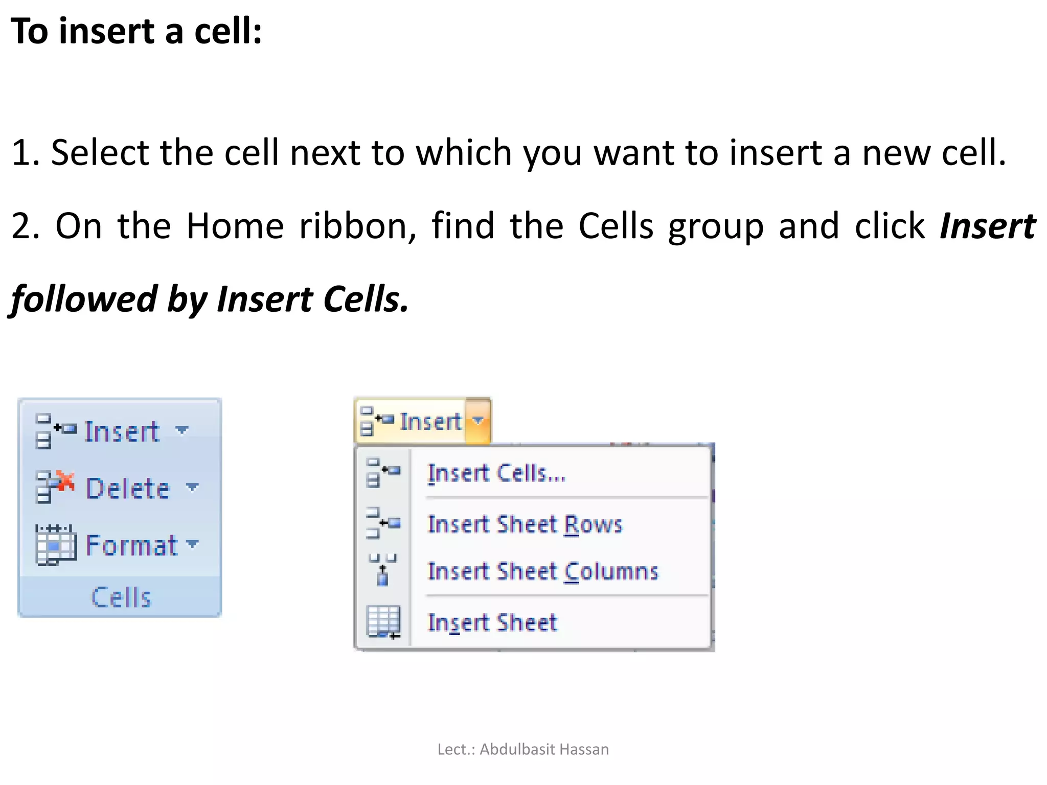
To insert acell:
1. Select the cell next to which you want to insert a new cell.
2. On the Home ribbon, find the Cells group and click Insert
followed by Insert Cells.
Lect.: Abdulbasit Hassan
59.
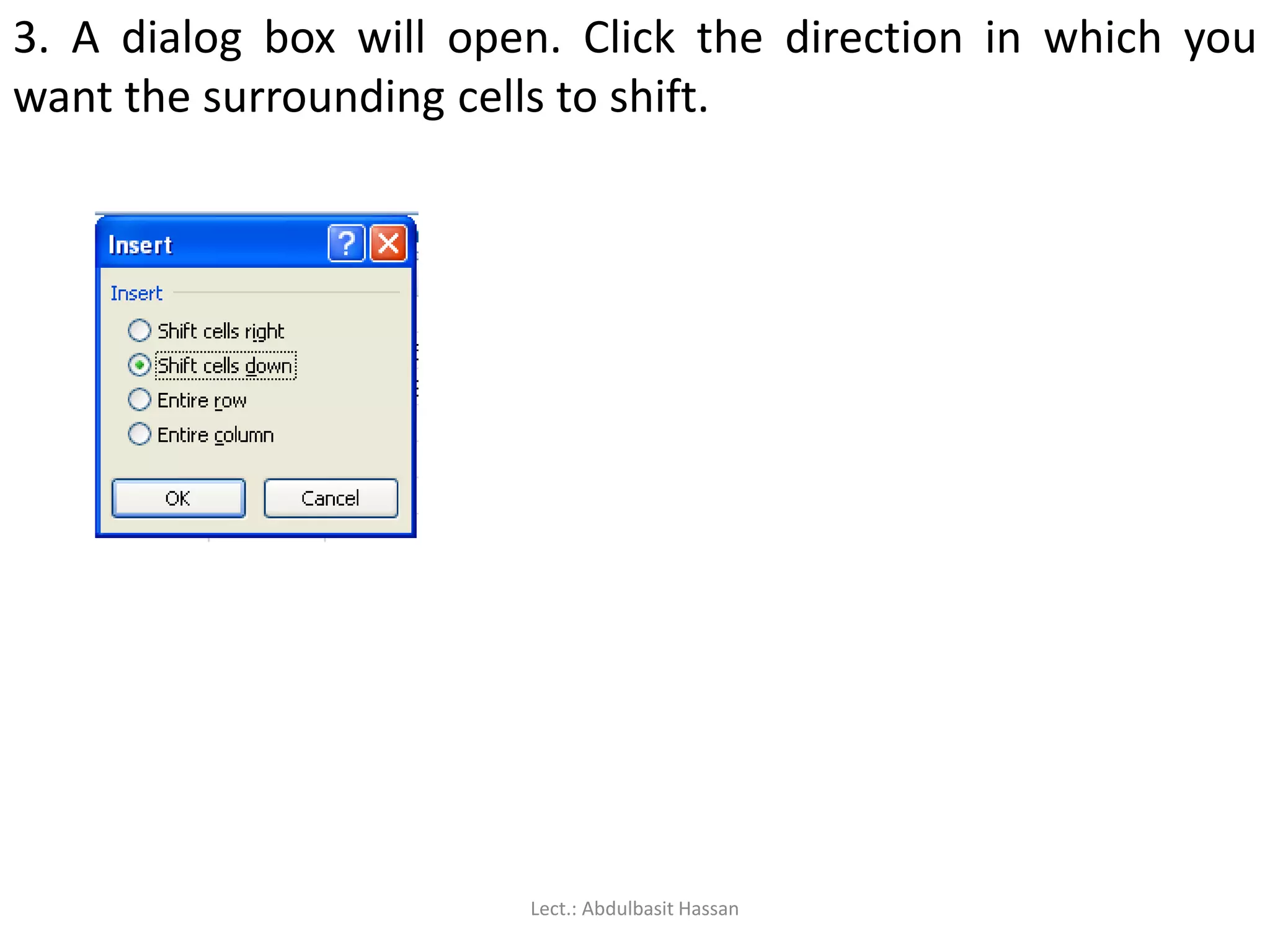
3. A dialogbox will open. Click the direction in which you
want the surrounding cells to shift.
Lect.: Abdulbasit Hassan
60.
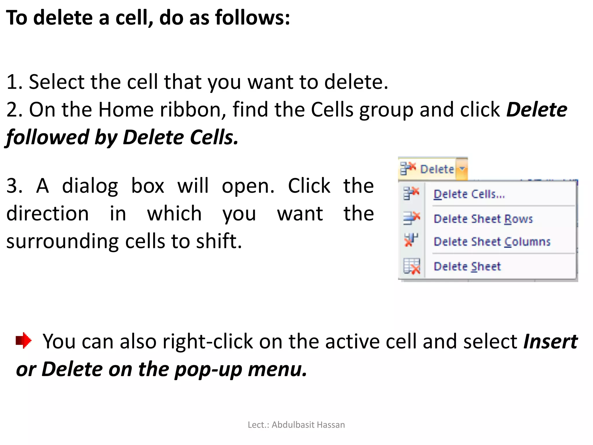
To delete acell, do as follows:
1. Select the cell that you want to delete.
2. On the Home ribbon, find the Cells group and click Delete
followed by Delete Cells.
3. A dialog box will open. Click the
direction in which you want the
surrounding cells to shift.
You can also right-click on the active cell and select Insert
or Delete on the pop-up menu.
Lect.: Abdulbasit Hassan
61.
Inserting or DeletingRows
When you insert a row, the new row will be positioned above the row
containing the active cell.
1. Select a cell in the row above which you want to insert a new row.
2. On the Home ribbon, find the Cells group and click Insert followed by
Insert Sheet Rows.
3. A new row will be inserted above the current row.
Lect.: Abdulbasit Hassan
62.
To delete arow, do as follows:
1. Select a cell in the row that you want to delete.
2. On the Home ribbon, find the Cells group and click Delete followed by
Delete Sheet Rows.
3. The row containing the active cell will be deleted. All the rows below
it will move up by one.
You can also right-click on the active cell and use the pop-up menu to
insert or delete a row.
Lect.: Abdulbasit Hassan
63.
Inserting or deletingcolumns:
When you insert a column, the new column will be positioned on the
left of the column containing the active cell.
1. Select a cell in the column to the left of which you want to insert a
new column.
2. On the Home ribbon, find the Cells group and click Insert followed by
Insert Sheet Columns.
3. A new column will be inserted to the left of the current column.
Lect.: Abdulbasit Hassan
64.
To delete acolumn, do as follows:
1. Select a cell in the column that you want to delete.
2. On the Home ribbon, find the Cells group and click Delete followed by
Delete Sheet Columns.
3. The column containing the active cell will be deleted. All the columns
on its right will move left by one.
You can also right-click on the active cell and use the pop-up menu to
insert or delete a column.
Lect.: Abdulbasit Hassan
To insert anew worksheet at the end of the existing
worksheets, just click the Insert Worksheet tab at the bottom
of the screen.
Lect.: Abdulbasit Hassan
68.
To insert anew worksheet before an existing worksheet, do
as follows:
1. Select the worksheet before which you want to insert a
new worksheet.
2. On the Home ribbon, find the Cells group and click Insert
followed by Insert Sheet.
3. A new worksheet will be inserted before the current
worksheet.
Lect.: Abdulbasit Hassan
69.
To delete aworksheet:
1. Select the worksheet that you want to delete.
2. On the Home ribbon, find the Cells group and click Delete
followed by Delete Sheet.
3. The current worksheet will be deleted.
Lect.: Abdulbasit Hassan
70.
Moving or copyinga worksheet:
Right-click on the worksheet tab, and select Move or Copy
from the pop-up menu. A dialog box will open:
The To Book field allows you to move or copy the current
worksheet to another workbook.
The Before Sheet field allows you to specify the new
position of the worksheet.
The Create a Copy checkbox lets you specify whether the
worksheet should be moved or copied.
Lect.: Abdulbasit Hassan
71.
Renaming a worksheet:
Right-clickon the
worksheet tab, and select
Rename from the pop-up
menu. Type the new
worksheet name and press
[ENTER].
Lect.: Abdulbasit Hassan
72.
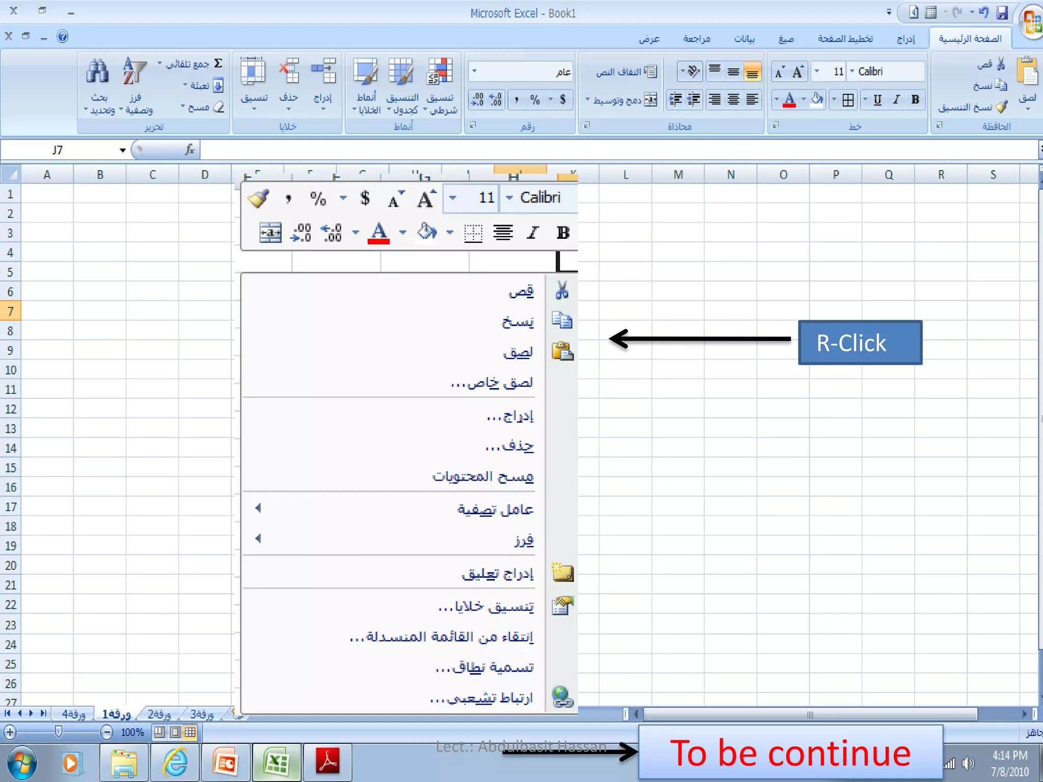
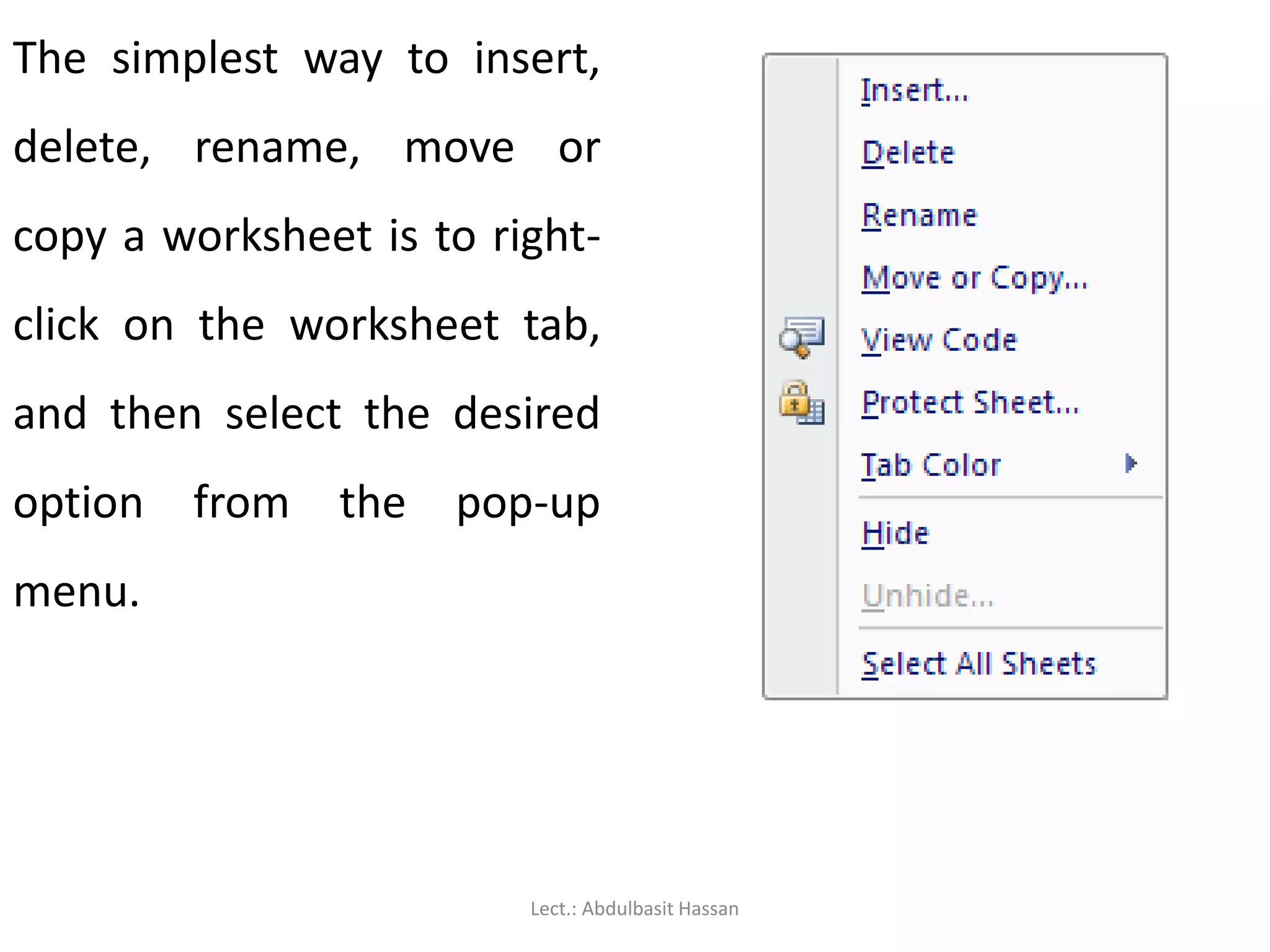
The simplest wayto insert,
delete, rename, move or
copy a worksheet is to right-
click on the worksheet tab,
and then select the desired
option from the pop-up
menu.
Lect.: Abdulbasit Hassan
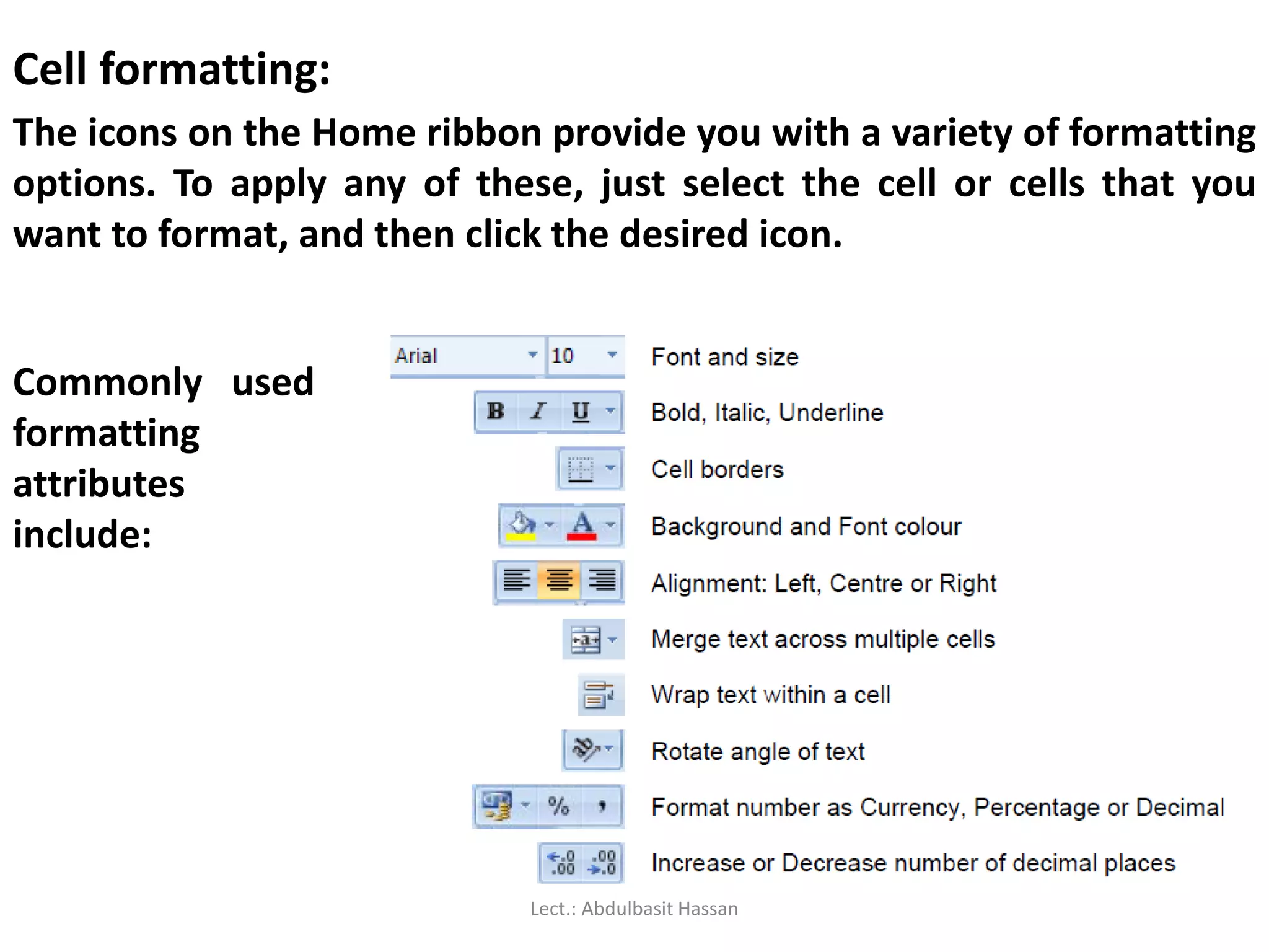
Cell formatting:
The iconson the Home ribbon provide you with a variety of formatting
options. To apply any of these, just select the cell or cells that you
want to format, and then click the desired icon.
Commonly used
formatting
attributes
include:
Lect.: Abdulbasit Hassan
75.
The Format Painterallows you to copy formatting attributes from one
cell to a range of cells.
1. Select the cell whose formatting attributes you want to copy.
2. Click on the Format Painter icon.
3. Select the cell or range of cells that you want to have the same
formatting attributes. The cell values will remain as before, but their
format will change.
Lect.: Abdulbasit Hassan
76.
Formatting rows andcolumns:
Any of the cell formatting options above can easily be
applied to all the cells contained in one or more rows or
columns.
Simply select the rows or columns by clicking on the row
or column labels, and then click on the formatting icons
that you want to apply.
Lect.: Abdulbasit Hassan
77.
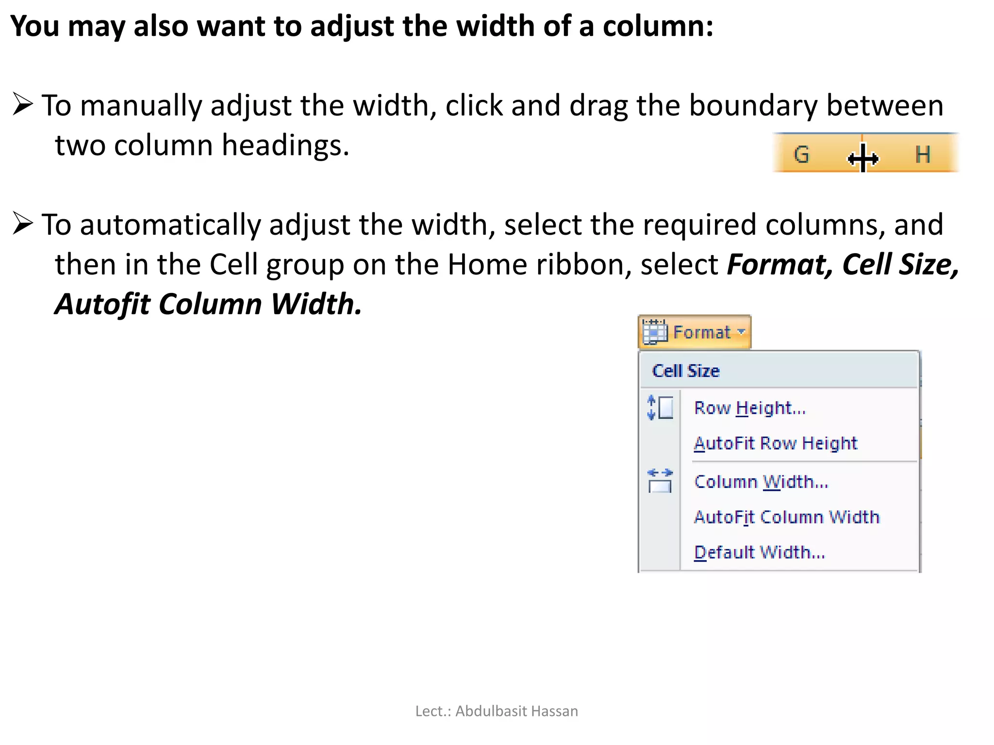
You may alsowant to adjust the width of a column:
To manually adjust the width, click and drag the boundary between
two column headings.
To automatically adjust the width, select the required columns, and
then in the Cell group on the Home ribbon, select Format, Cell Size,
Autofit Column Width.
Lect.: Abdulbasit Hassan
78.
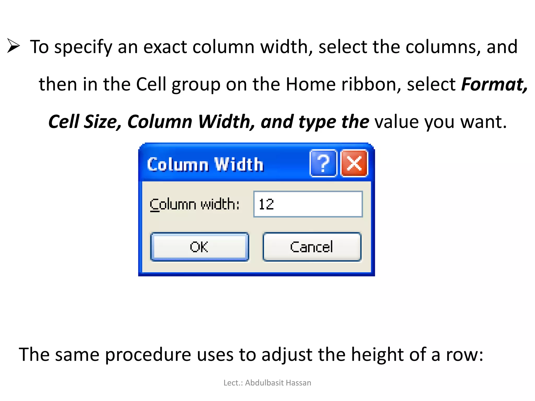
To specifyan exact column width, select the columns, and
then in the Cell group on the Home ribbon, select Format,
Cell Size, Column Width, and type the value you want.
The same procedure uses to adjust the height of a row:
Lect.: Abdulbasit Hassan
79.
Hiding Rows andColumns:
If your spreadsheet contains sensitive data that you don’t want
displayed on the screen or included in printouts, then you can hide
the corresponding rows or columns.
The cell values can still be used for calculations, but will be hidden
from view.
The easiest way to hide or unhide a row or column is to select the
row or column heading, right-click to view the pop-up menu, and
then select Hide or Unhide.
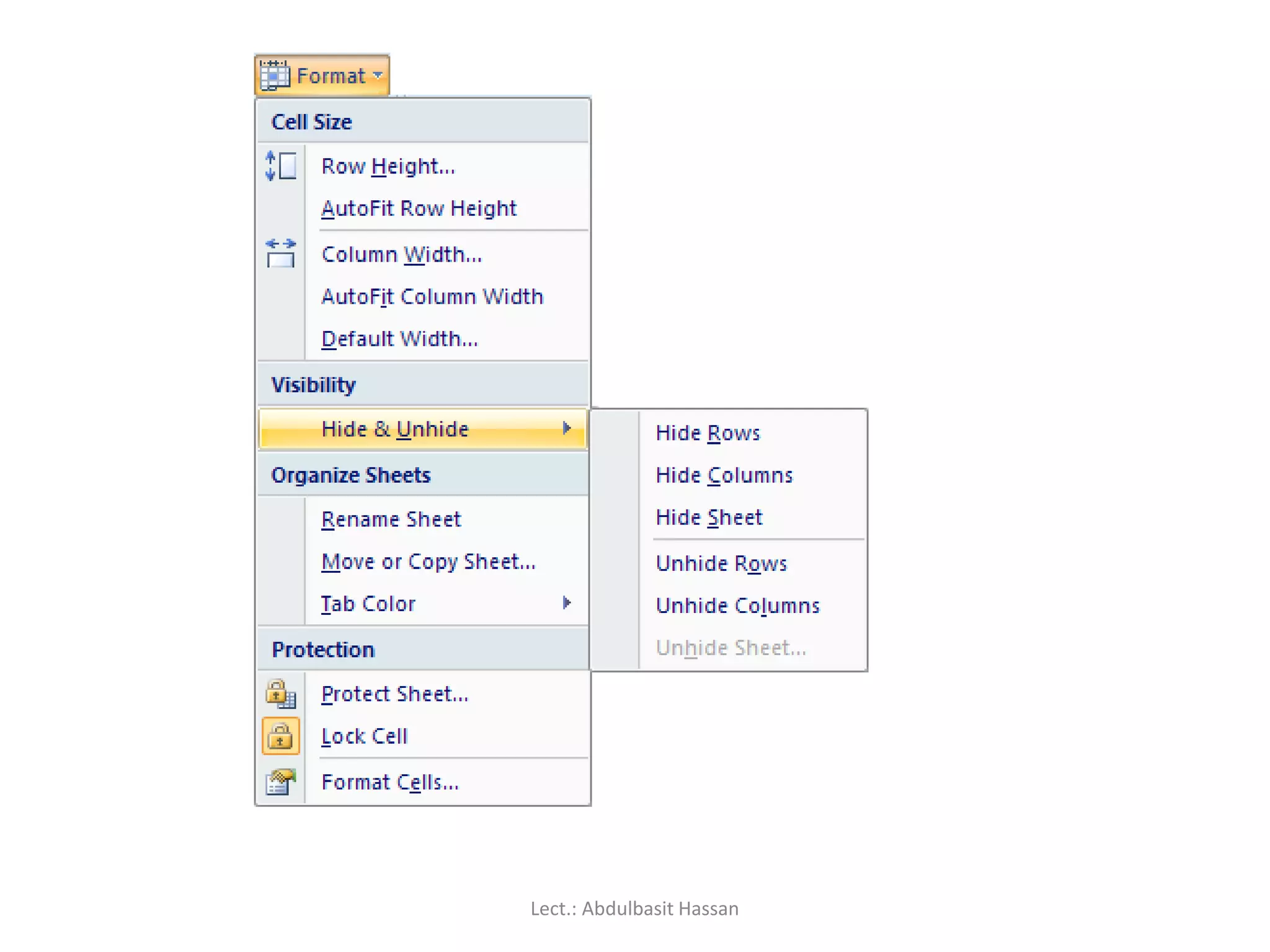
Alternatively, you can click the Format icon on the Home ribbon,
and select the Hide & Unhide option.
Lect.: Abdulbasit Hassan
Keeping row andcolumn headings in view:
If you scroll through a lot of data in a worksheet, you’ll
probably lose sight of the column headings as they disappear
off the top of your “page”. This can make life really difficult –
imagine trying to check a student’s result for tutorial 8 in row
183 of the worksheet! And it’s even more difficult if the
student’s name in column A has scrolled off the left edge of
the window.
Lect.: Abdulbasit Hassan
82.
The Freeze Panesfeature allows you to specify particular rows
and columns that will always remain visible as you scroll
through the worksheet. And it’s easy to do!
Lect.: Abdulbasit Hassan
83.
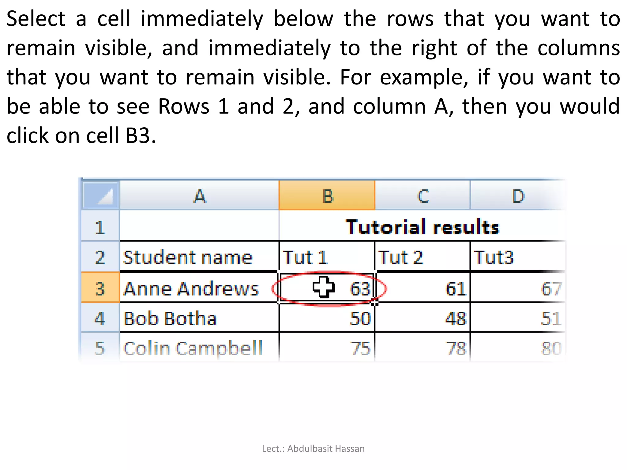
Select a cellimmediately below the rows that you want to
remain visible, and immediately to the right of the columns
that you want to remain visible. For example, if you want to
be able to see Rows 1 and 2, and column A, then you would
click on cell B3.
Lect.: Abdulbasit Hassan
84.
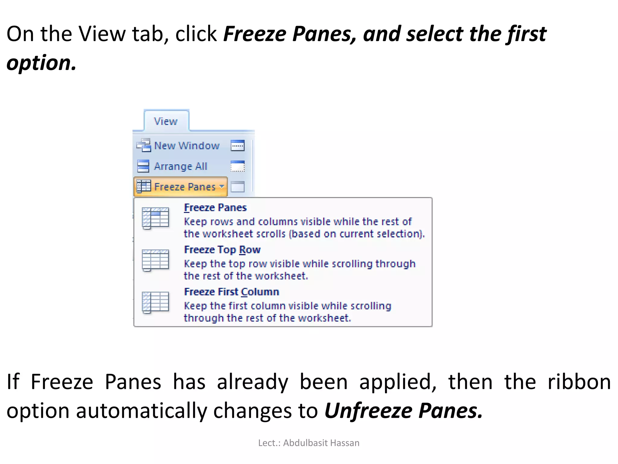
On the Viewtab, click Freeze Panes, and select the first
option.
If Freeze Panes has already been applied, then the ribbon
option automatically changes to Unfreeze Panes.
Lect.: Abdulbasit Hassan
In this sectionI’m going to explain how to construct a
formula, and give you some guidelines to ensure that your
formulas work correctly.
Lect.: Abdulbasit Hassan
87.
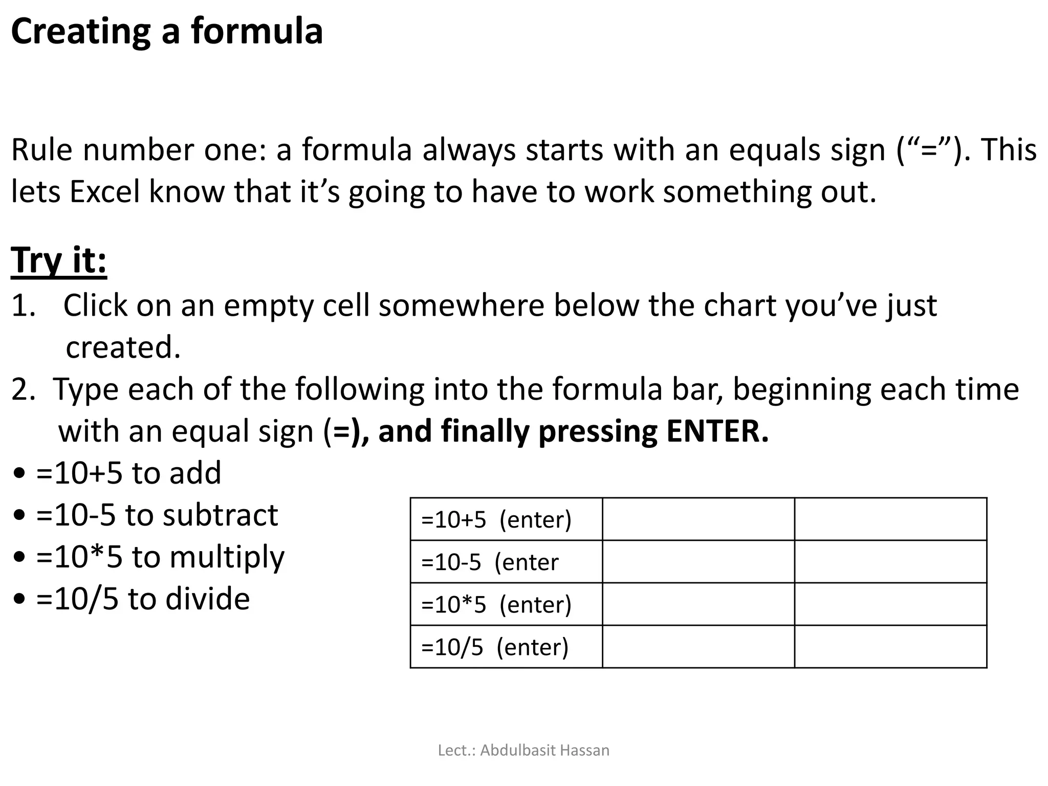
Creating a formula
Rulenumber one: a formula always starts with an equals sign (“=”). This
lets Excel know that it’s going to have to work something out.
Try it:
1. Click on an empty cell somewhere below the chart you’ve just
created.
2. Type each of the following into the formula bar, beginning each time
with an equal sign (=), and finally pressing ENTER.
• =10+5 to add
• =10-5 to subtract
• =10*5 to multiply
• =10/5 to divide
=10+5 (enter)
=10-5 (enter
=10*5 (enter)
=10/5 (enter)
Lect.: Abdulbasit Hassan
88.
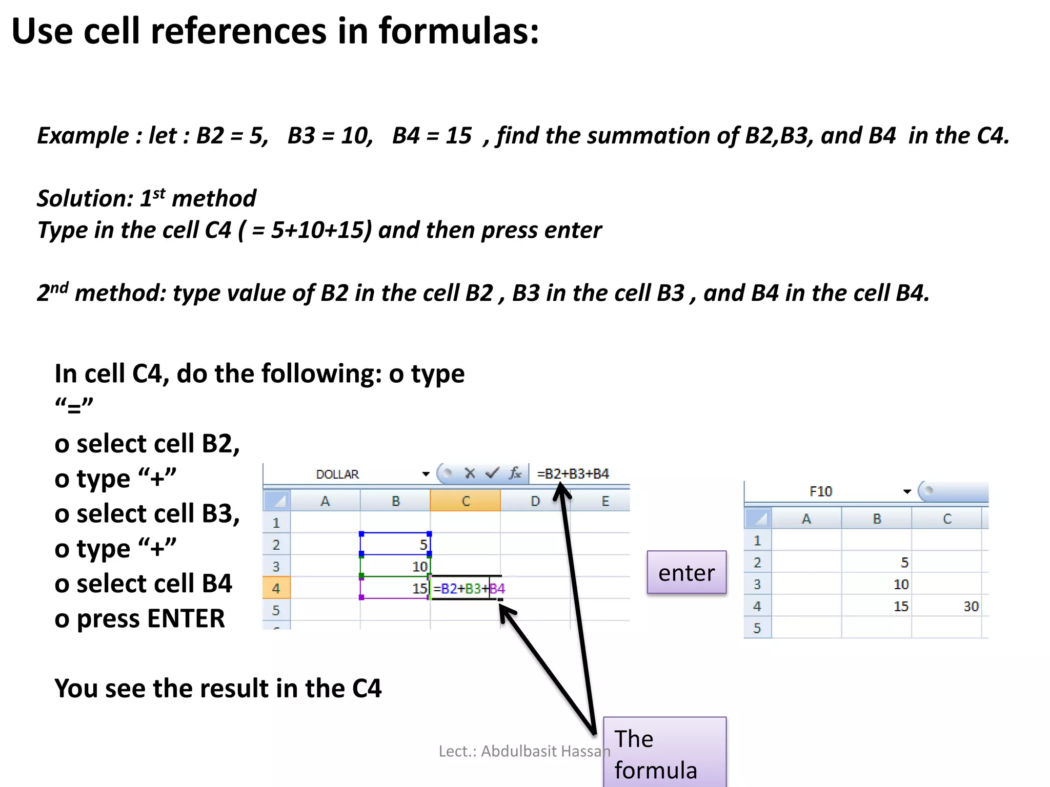
Use cell referencesin formulas:
Example : let : B2 = 5, B3 = 10, B4 = 15 , find the summation of B2,B3, and B4 in the C4.
Solution: 1st method
Type in the cell C4 ( = 5+10+15) and then press enter
2nd method: type value of B2 in the cell B2 , B3 in the cell B3 , and B4 in the cell B4.
In cell C4, do the following: o type
“=”
o select cell B2,
o type “+”
o select cell B3,
o type “+”
o select cell B4
o press ENTER
You see the result in the C4
enter
The
formula
Lect.: Abdulbasit Hassan
89.
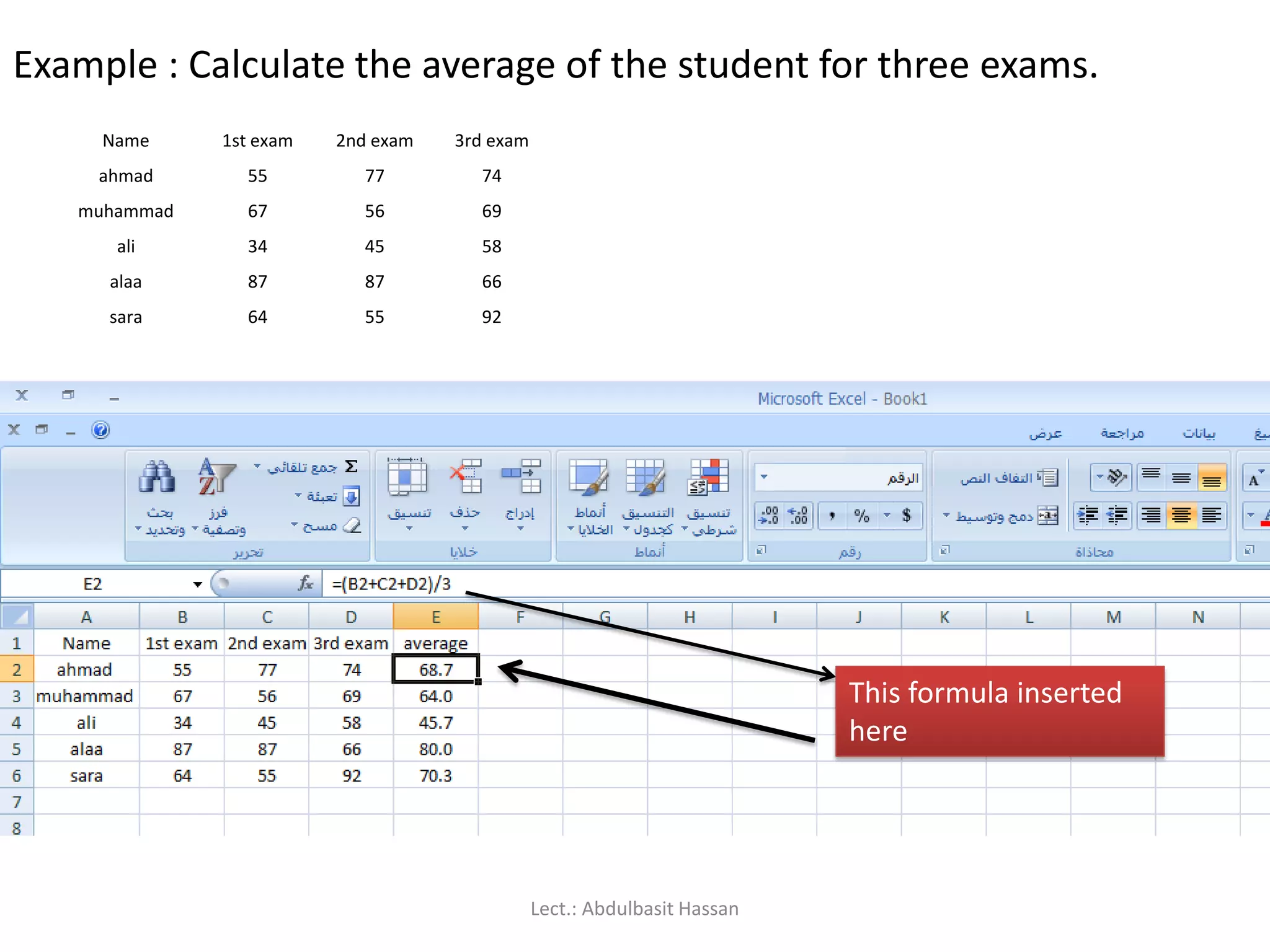
Example : Calculatethe average of the student for three exams.
Name 1st exam 2nd exam 3rd exam
ahmad 55 77 74
muhammad 67 56 69
ali 34 45 58
alaa 87 87 66
sara 64 55 92
This formula inserted
here
Lect.: Abdulbasit Hassan
90.
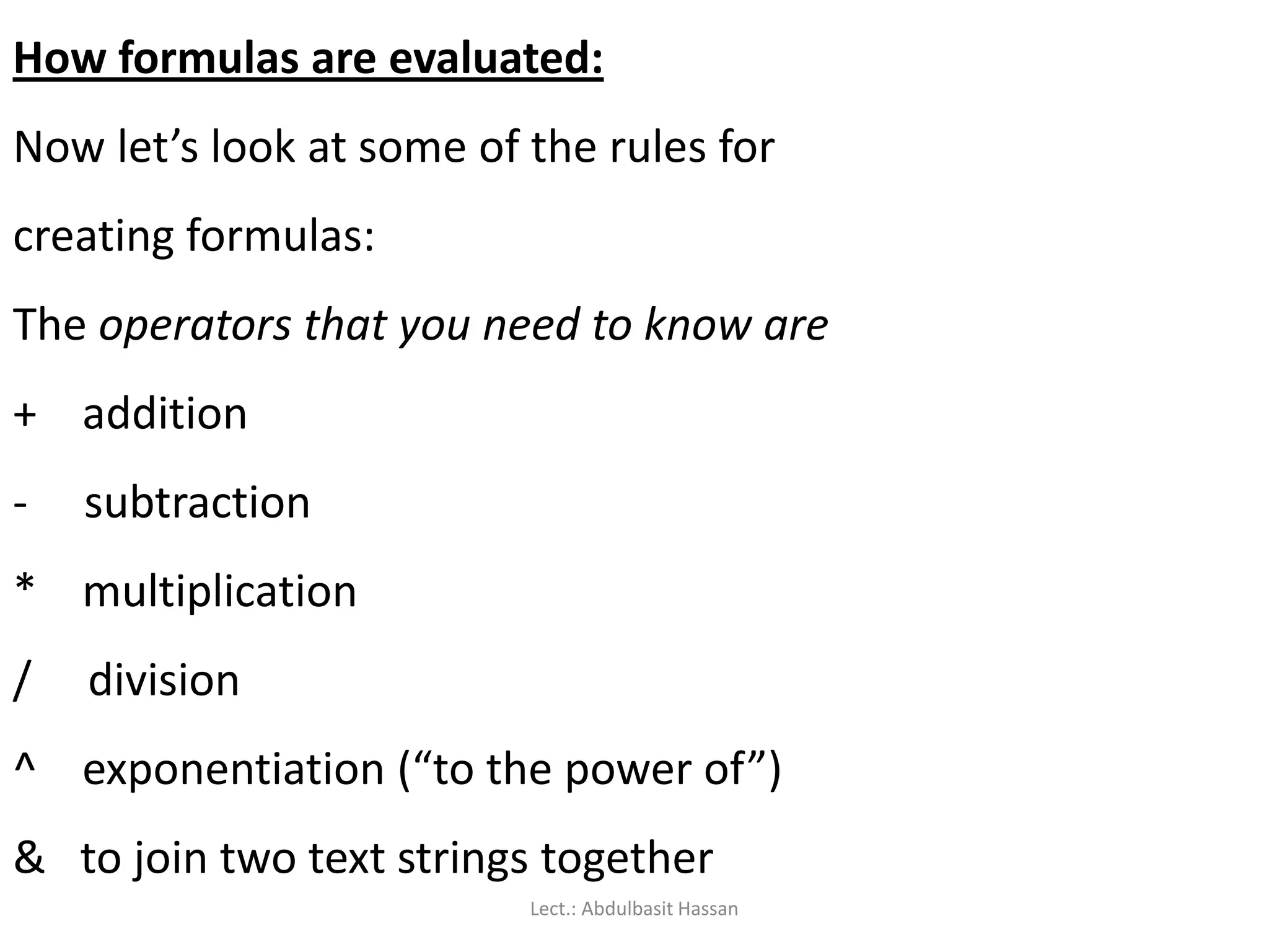
How formulas areevaluated:
Now let’s look at some of the rules for
creating formulas:
The operators that you need to know are
+ addition
- subtraction
* multiplication
/ division
^ exponentiation (“to the power of”)
& to join two text strings together
Lect.: Abdulbasit Hassan
91.
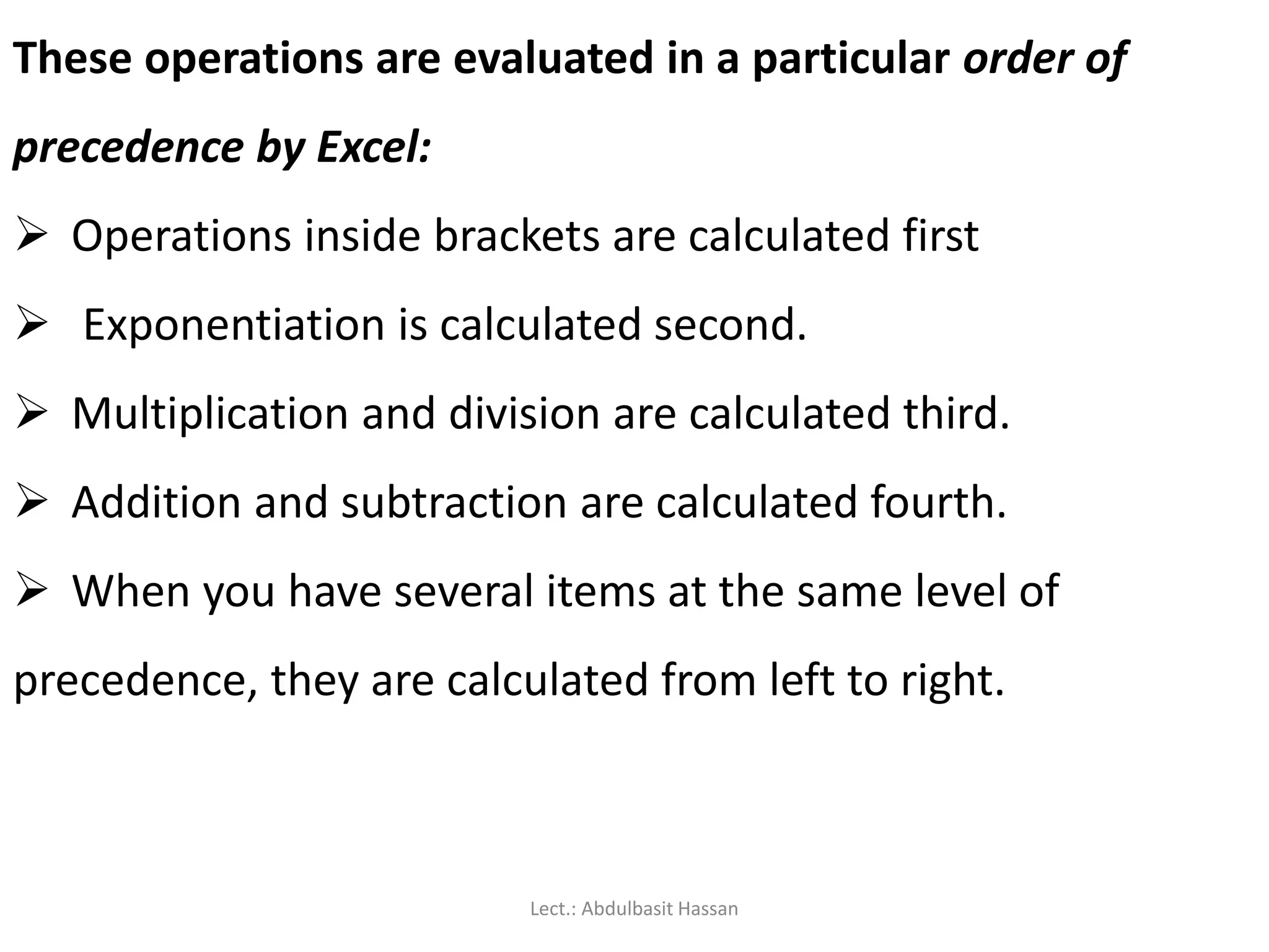
These operations areevaluated in a particular order of
precedence by Excel:
Operations inside brackets are calculated first
Exponentiation is calculated second.
Multiplication and division are calculated third.
Addition and subtraction are calculated fourth.
When you have several items at the same level of
precedence, they are calculated from left to right.
Lect.: Abdulbasit Hassan
92.
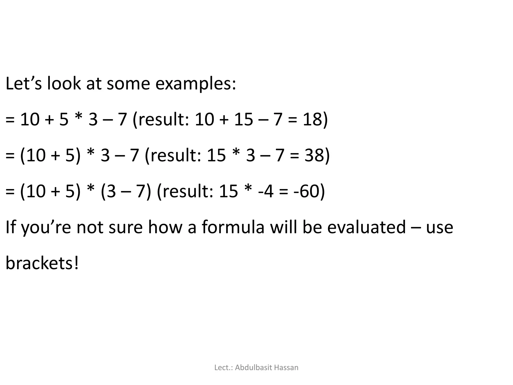
Let’s look atsome examples:
= 10 + 5 * 3 – 7 (result: 10 + 15 – 7 = 18)
= (10 + 5) * 3 – 7 (result: 15 * 3 – 7 = 38)
= (10 + 5) * (3 – 7) (result: 15 * -4 = -60)
If you’re not sure how a formula will be evaluated – use
brackets!
Lect.: Abdulbasit Hassan
93.
Functions are predefinedformulas that are designed to
perform specialized types of calculations. For example, the
Sum function is designed to add values in the cells specified.
For example =Sum(A1:A5) or =Average(C2:E2)
Lect.: Abdulbasit Hassan
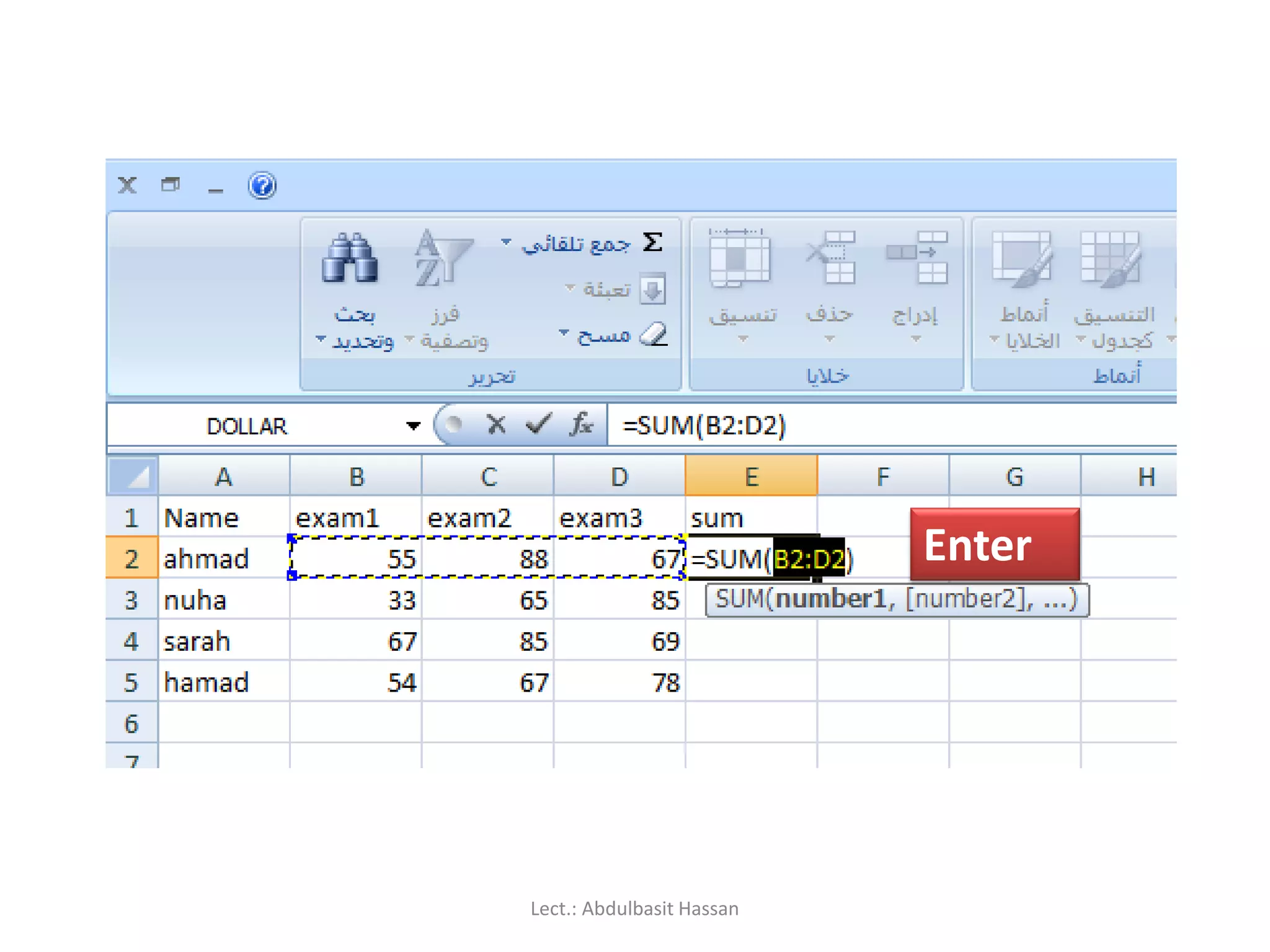
Using AutoSum:
Because additionis the most frequently used Excel function, a shortcut
has been provided to quickly add a set of numbers:
1. Select the cell where you want the total to appear.
2. Click on the Sum button on the Home ribbon.
3. Check that the correct set of numbers has been selected (indicated by
a dotted line). If not, then drag to select a different set of numbers.
4. Press [ENTER] and the total will be calculated.
Lect.: Abdulbasit Hassan
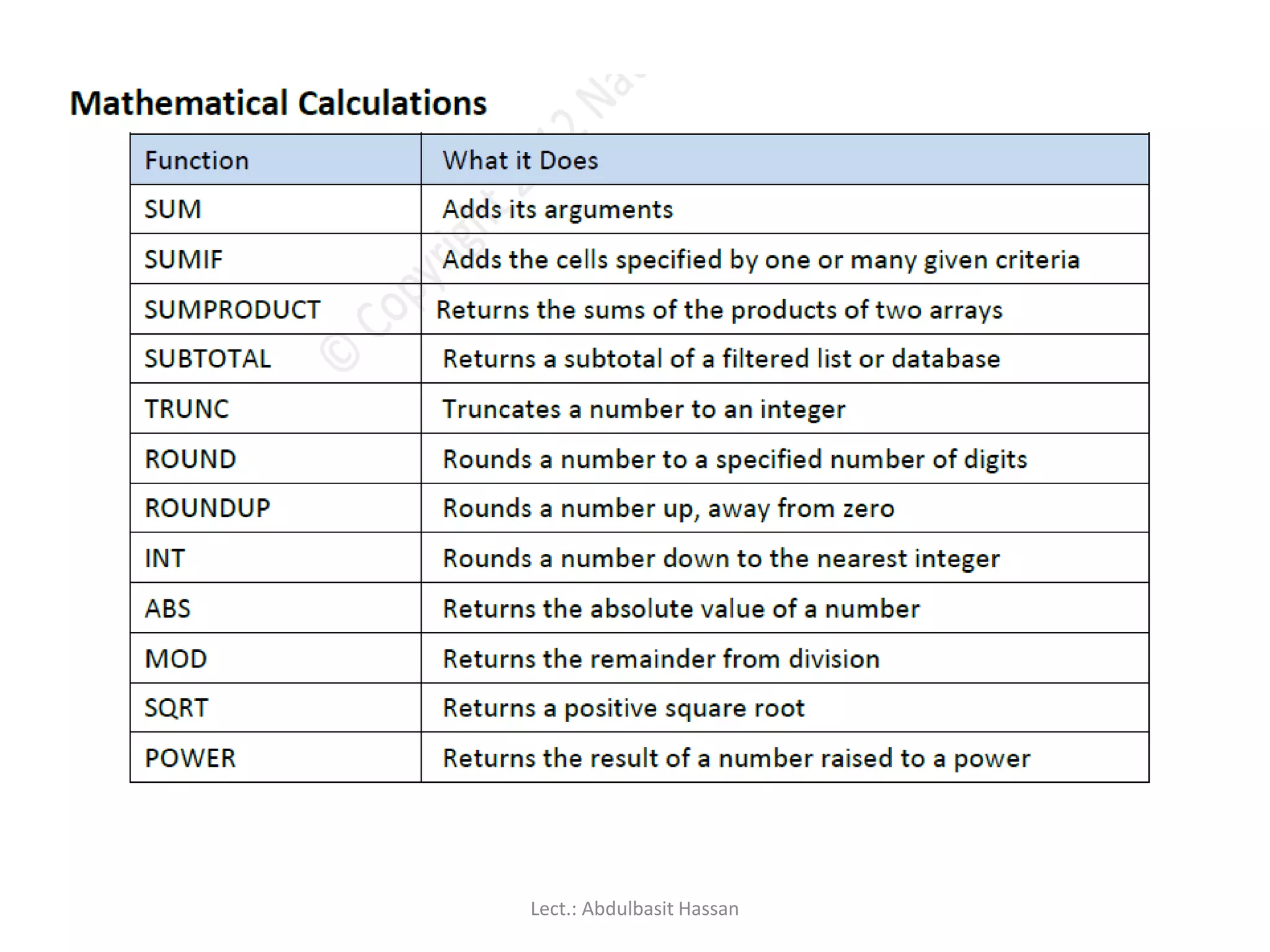
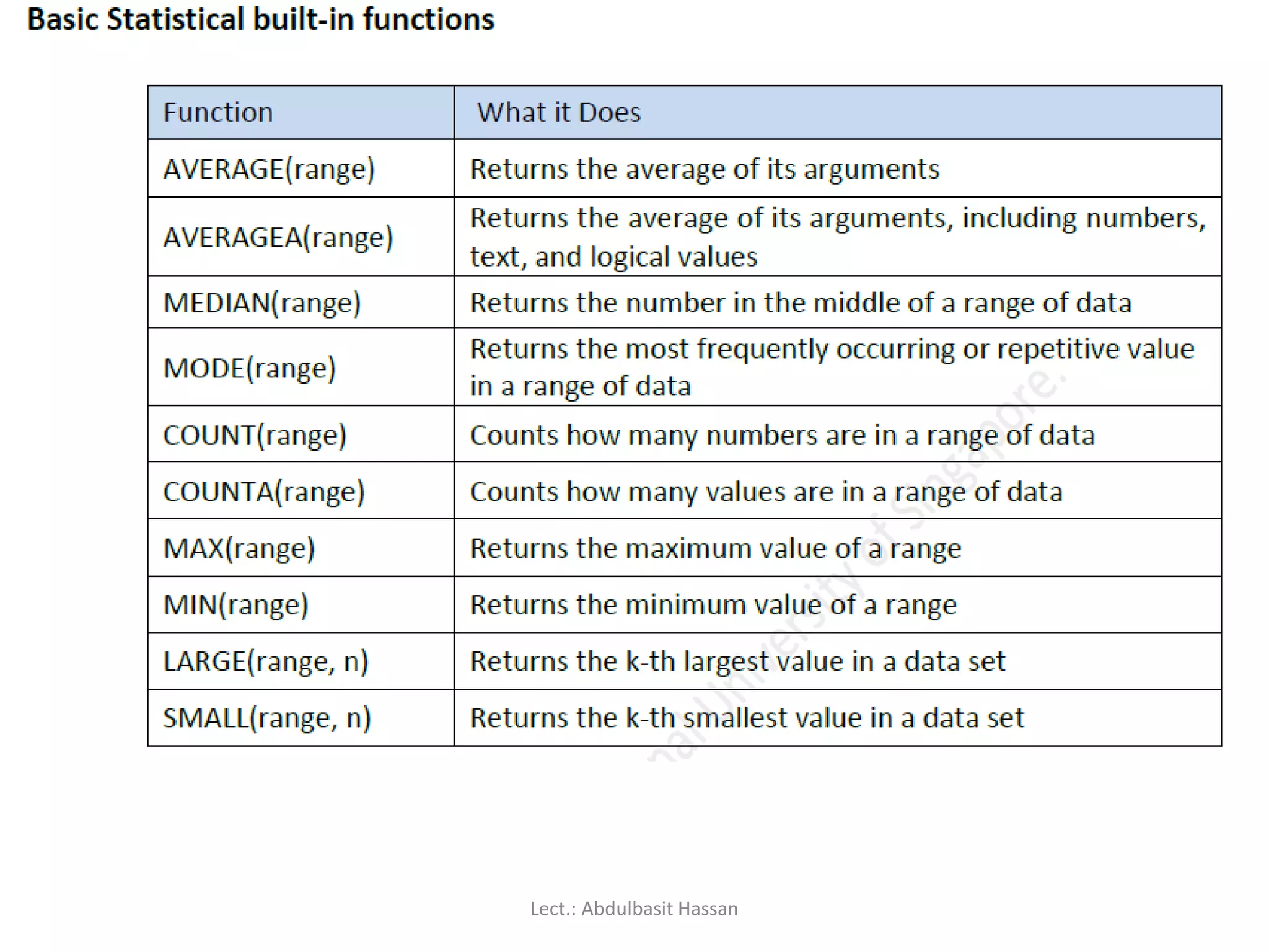
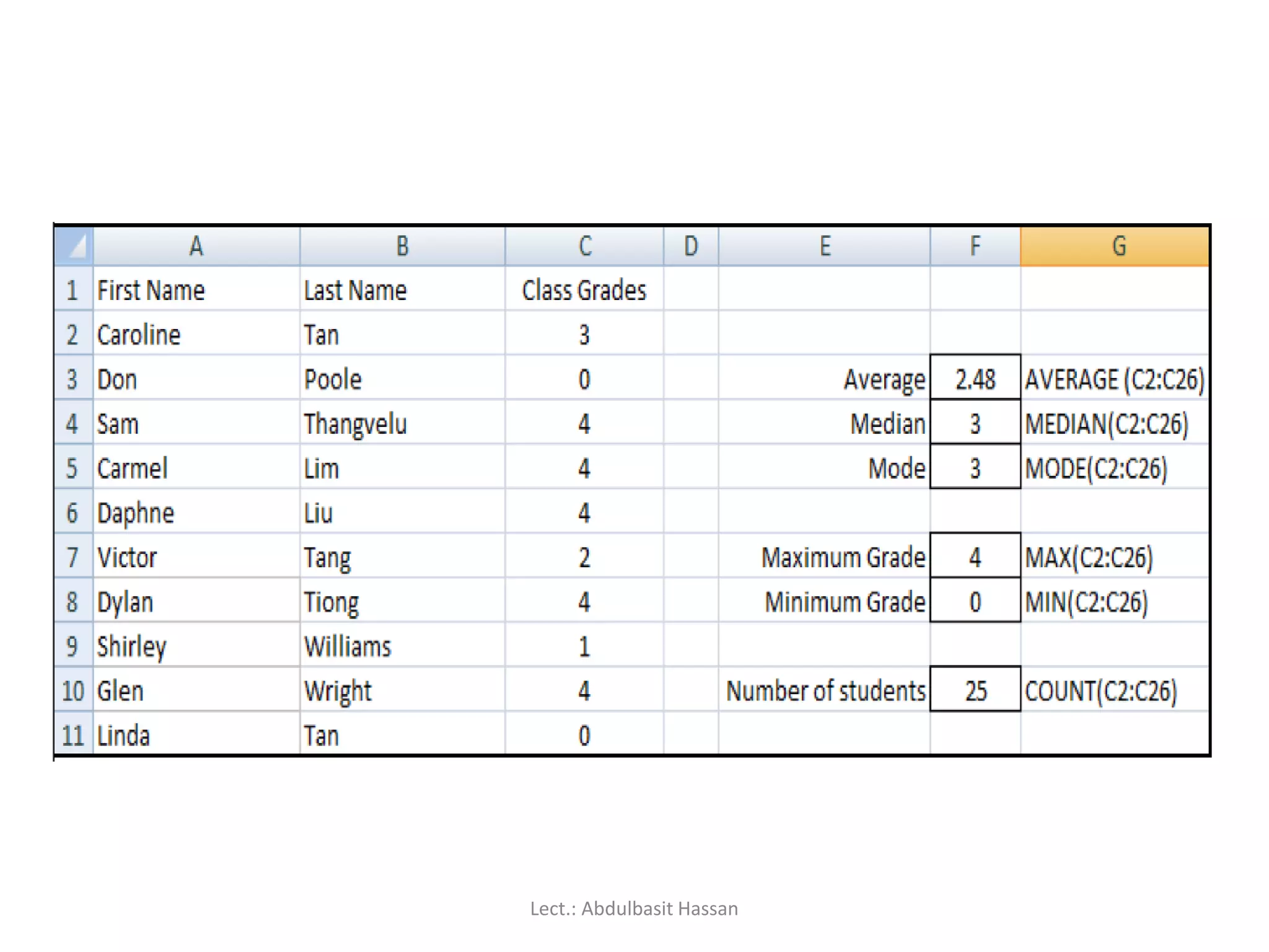
Basic functions:
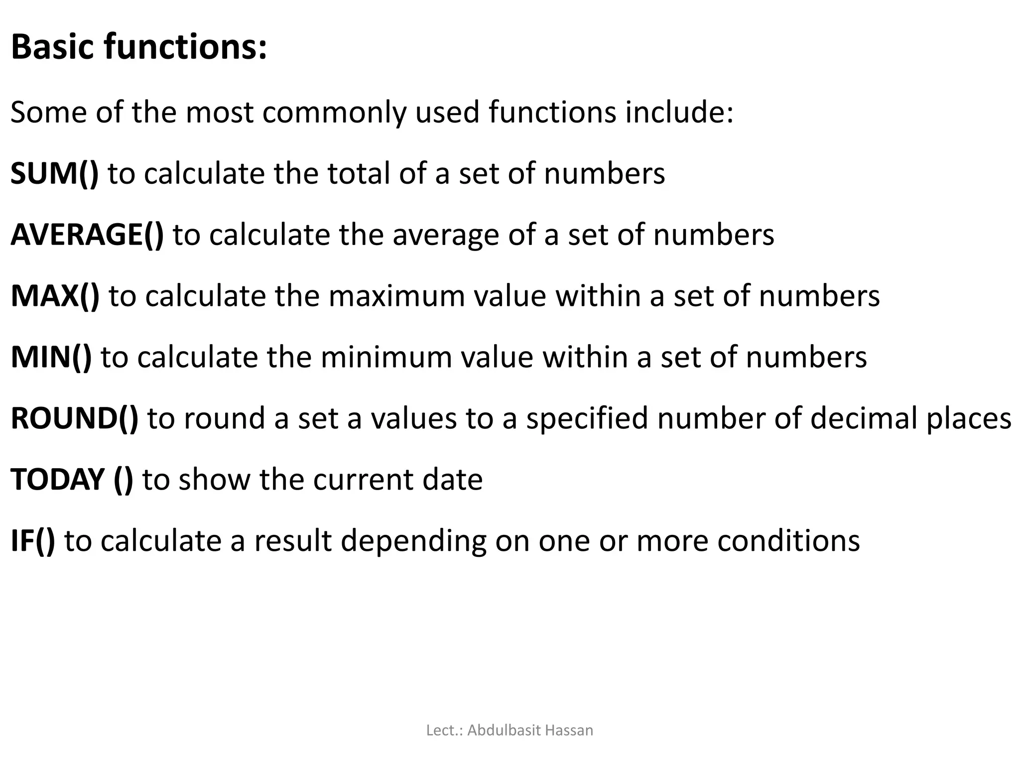
Some ofthe most commonly used functions include:
SUM() to calculate the total of a set of numbers
AVERAGE() to calculate the average of a set of numbers
MAX() to calculate the maximum value within a set of numbers
MIN() to calculate the minimum value within a set of numbers
ROUND() to round a set a values to a specified number of decimal places
TODAY () to show the current date
IF() to calculate a result depending on one or more conditions
Lect.: Abdulbasit Hassan
105.
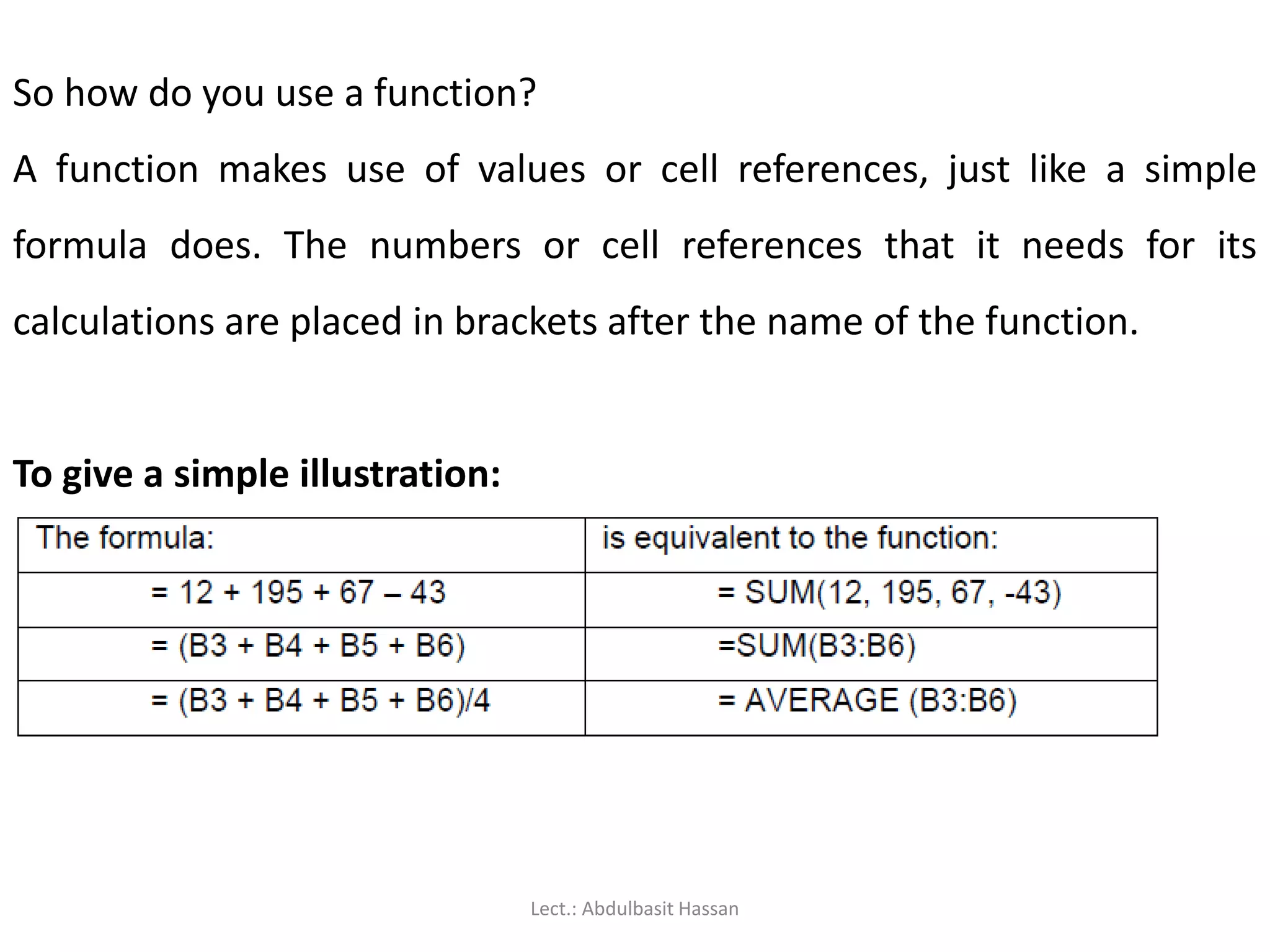
So how doyou use a function?
A function makes use of values or cell references, just like a simple
formula does. The numbers or cell references that it needs for its
calculations are placed in brackets after the name of the function.
To give a simple illustration:
Lect.: Abdulbasit Hassan
106.
Several popular functionsare available to you directly from the Home
ribbon.
1. Select the cell where you want the result of the calculation to be
displayed.
2. Click the drop-down arrow next to the Sum button.
3. Click on the function that you want.
4. Confirm the range of cells that the function should use in its
calculation.
5. Press [ENTER]. The result of the calculation will be shown in the active
cell.
Lect.: Abdulbasit Hassan
107.
As an example,to calculate the average for the following set of tutorial
results, you would:
1. Click on cell F3 to make it active.
2. Click on the arrow next to the Sum button, and select Average.
3. Press [ENTER] to accept the range of cells that is suggested (B3:E3).
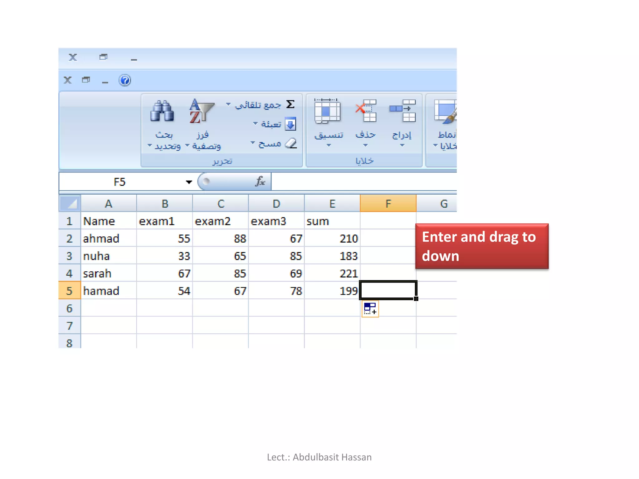
That’s it! You can now copy the formula in cell F3 down to cells F4 and
F5 – using relative addressing because you want a different set of
tutorial marks to be used for each student.
Lect.: Abdulbasit Hassan
108.
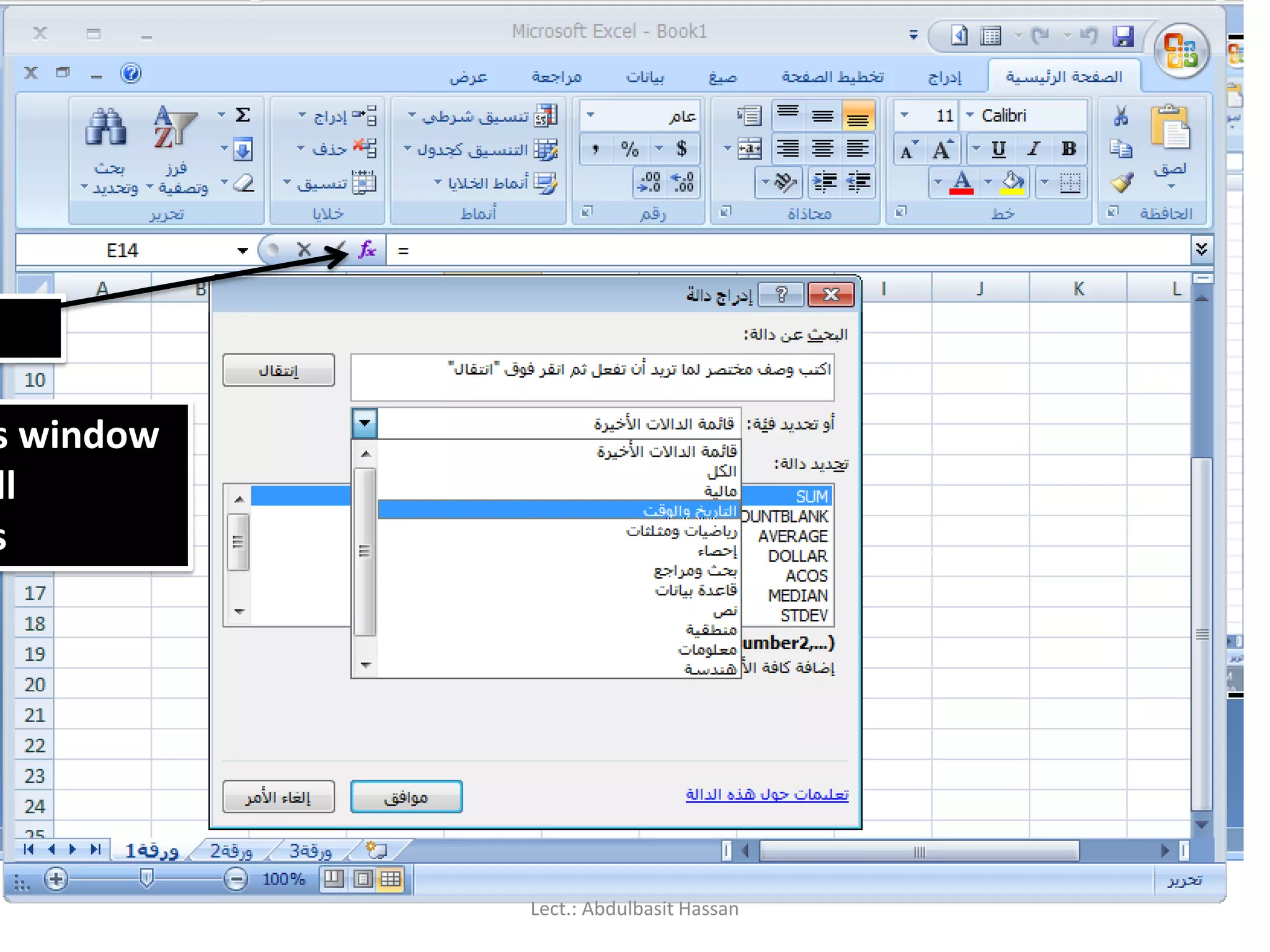
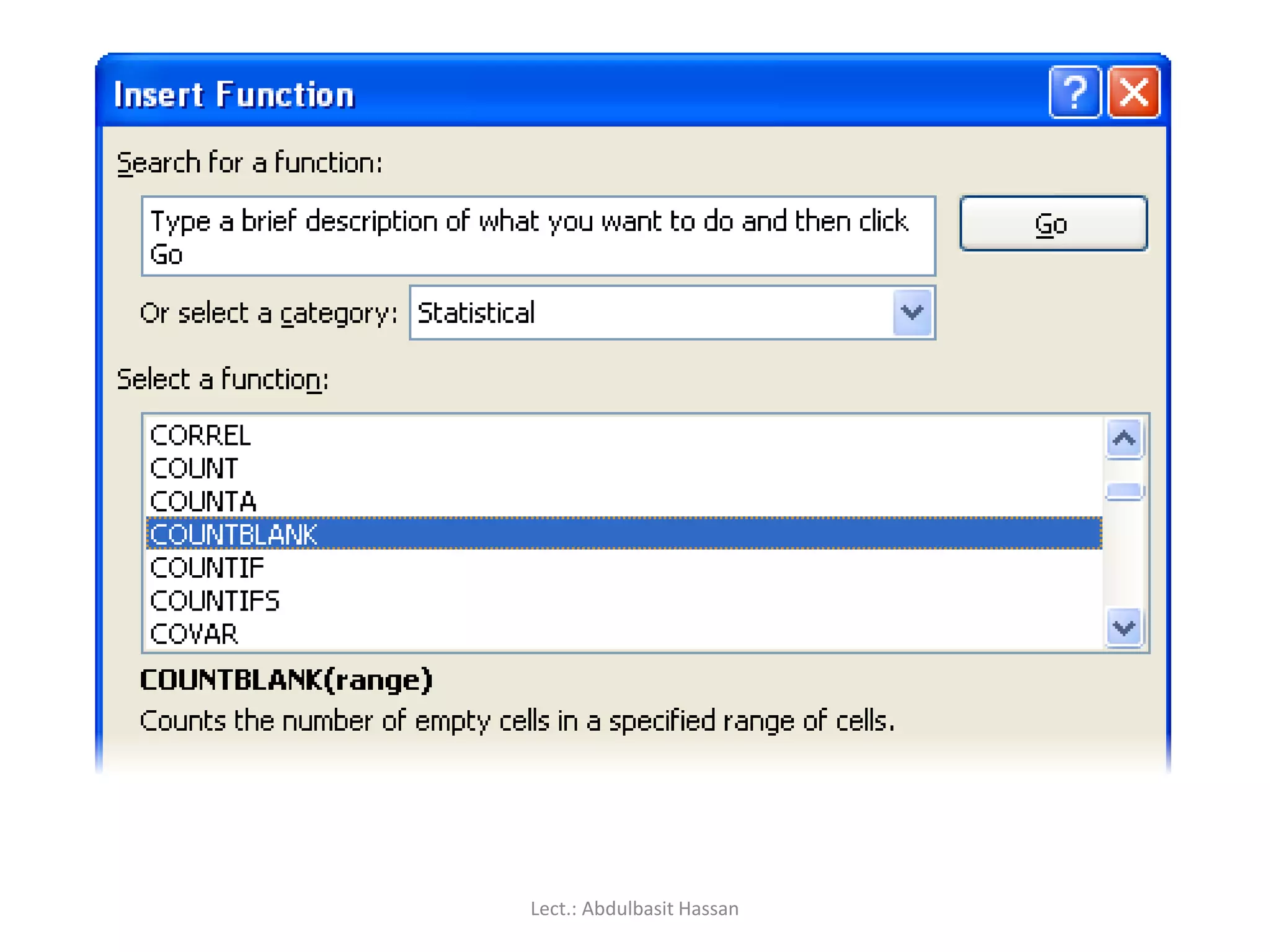
If you wantto use a function that isn’t directly available from the drop-
down list, then you can click on More Functions to open the Insert
Function dialog box. Another way to open this dialog box is to click the
Insert Function icon on the immediate left of the formula bar.
The Insert Function dialog box displays a list of functions within a
selected function category. If you select a function it will briefly describe
the purpose and structure of the function.
Lect.: Abdulbasit Hassan
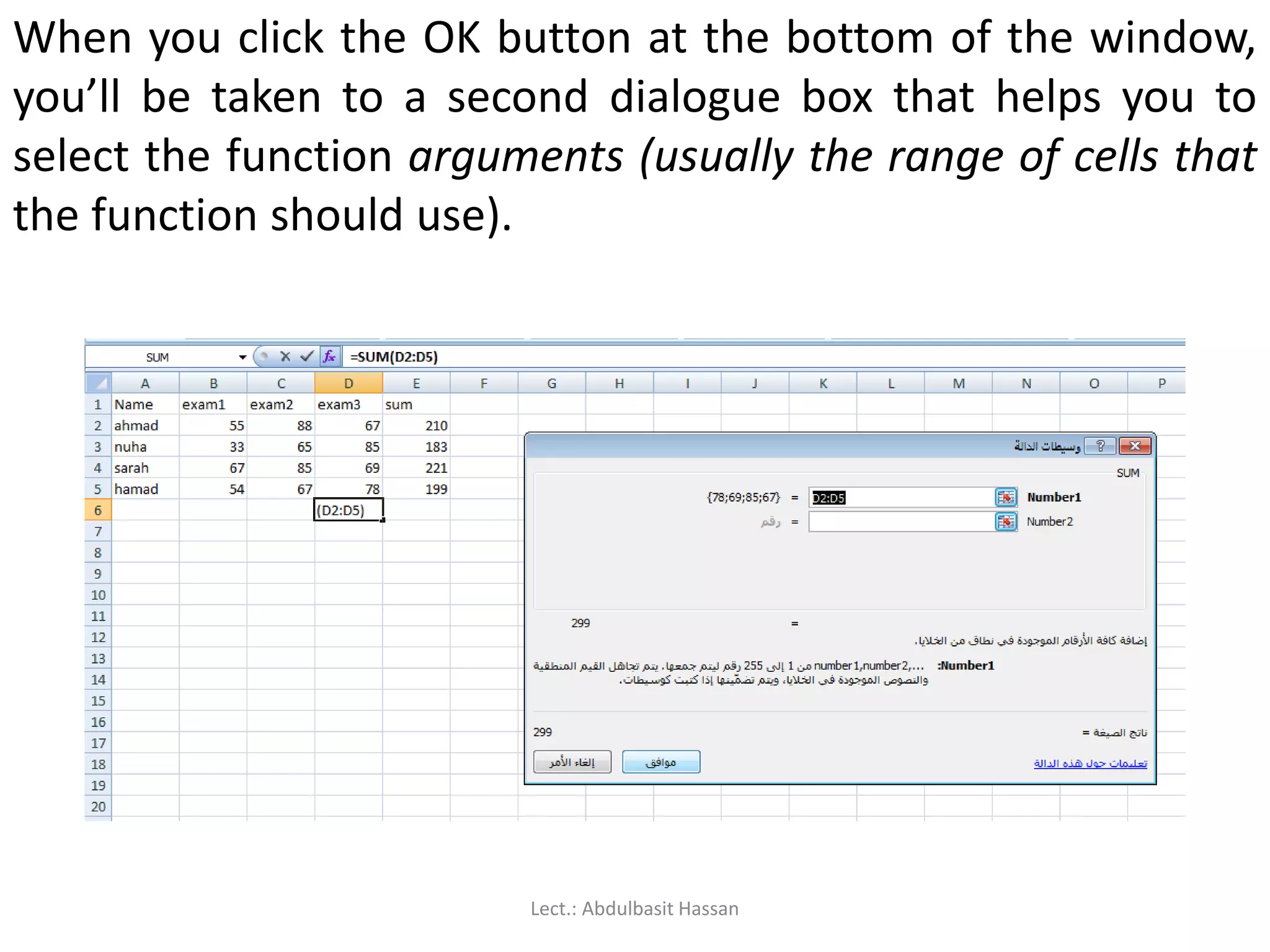
When you clickthe OK button at the bottom of the window,
you’ll be taken to a second dialogue box that helps you to
select the function arguments (usually the range of cells that
the function should use).
Lect.: Abdulbasit Hassan
111.
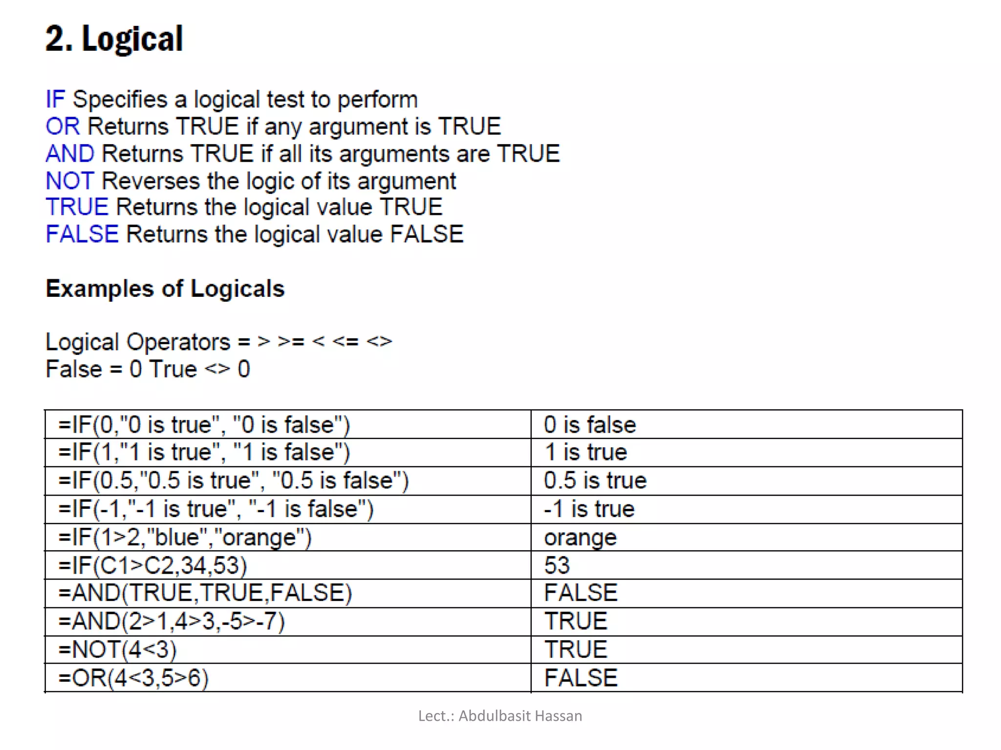
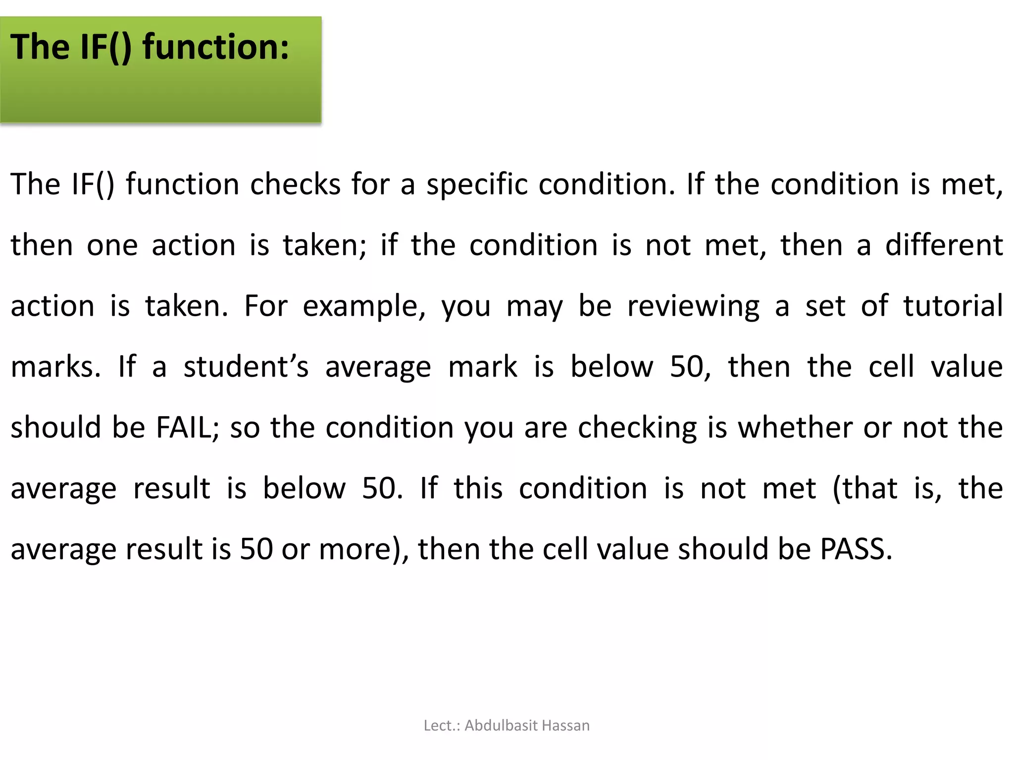
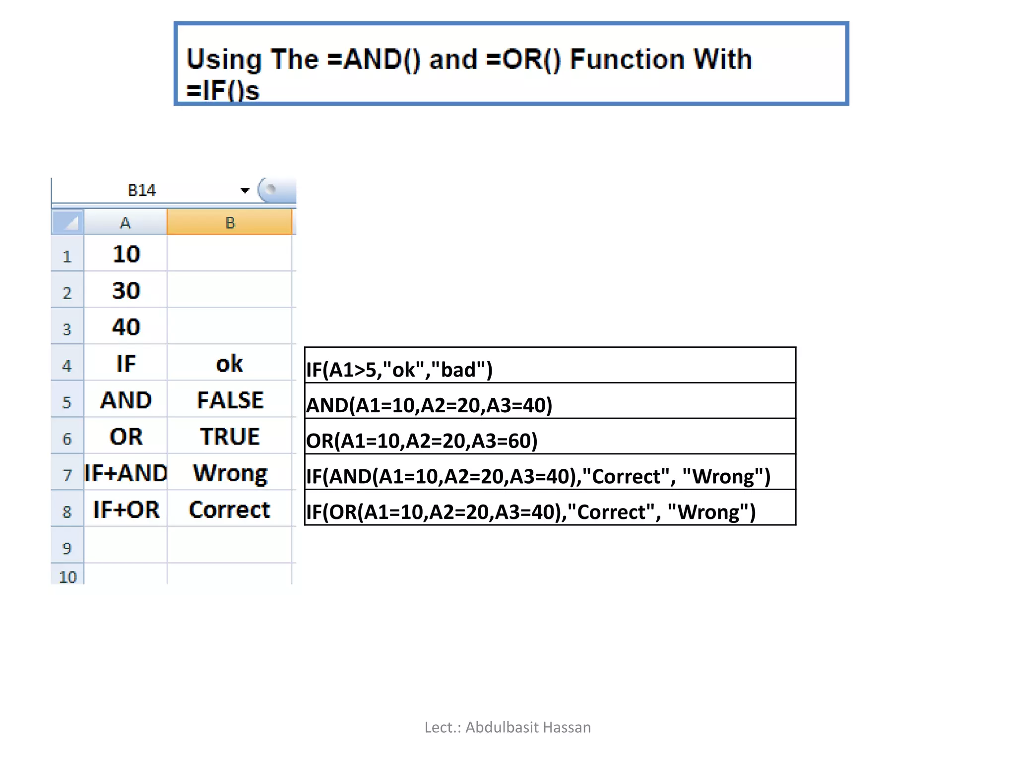
The IF() function:
TheIF() function checks for a specific condition. If the condition is met,
then one action is taken; if the condition is not met, then a different
action is taken. For example, you may be reviewing a set of tutorial
marks. If a student’s average mark is below 50, then the cell value
should be FAIL; so the condition you are checking is whether or not the
average result is below 50. If this condition is not met (that is, the
average result is 50 or more), then the cell value should be PASS.
Lect.: Abdulbasit Hassan
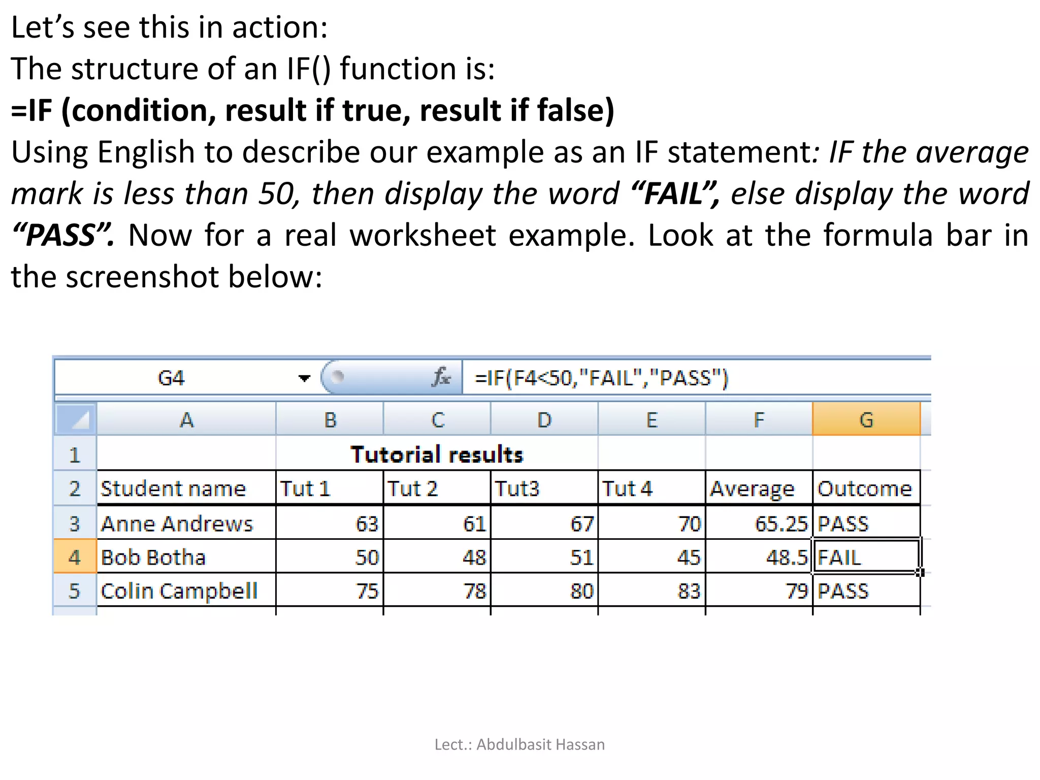
Let’s see thisin action:
The structure of an IF() function is:
=IF (condition, result if true, result if false)
Using English to describe our example as an IF statement: IF the average
mark is less than 50, then display the word “FAIL”, else display the word
“PASS”. Now for a real worksheet example. Look at the formula bar in
the screenshot below:
Lect.: Abdulbasit Hassan
114.
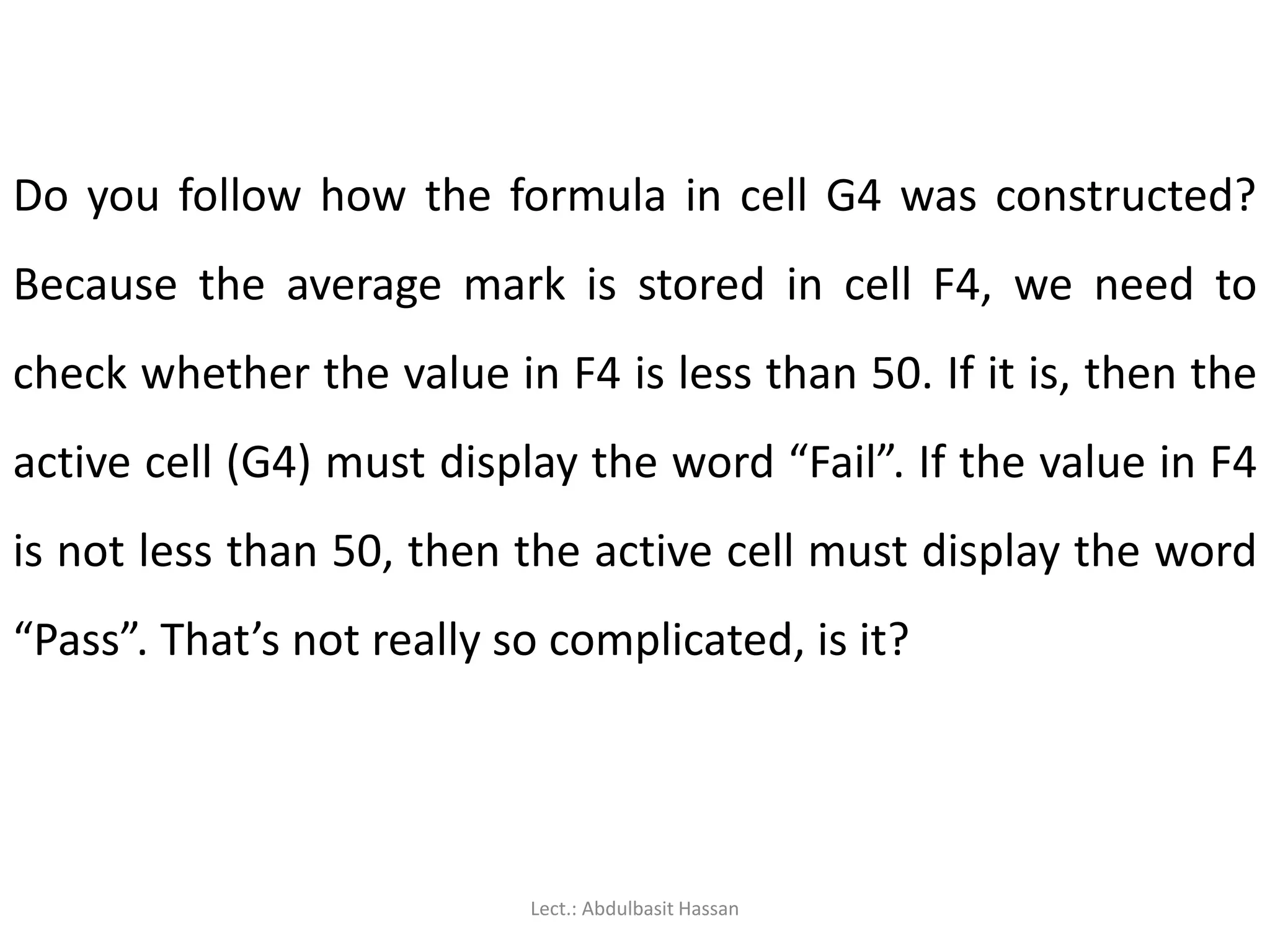
Do you followhow the formula in cell G4 was constructed?
Because the average mark is stored in cell F4, we need to
check whether the value in F4 is less than 50. If it is, then the
active cell (G4) must display the word “Fail”. If the value in F4
is not less than 50, then the active cell must display the word
“Pass”. That’s not really so complicated, is it?
Lect.: Abdulbasit Hassan
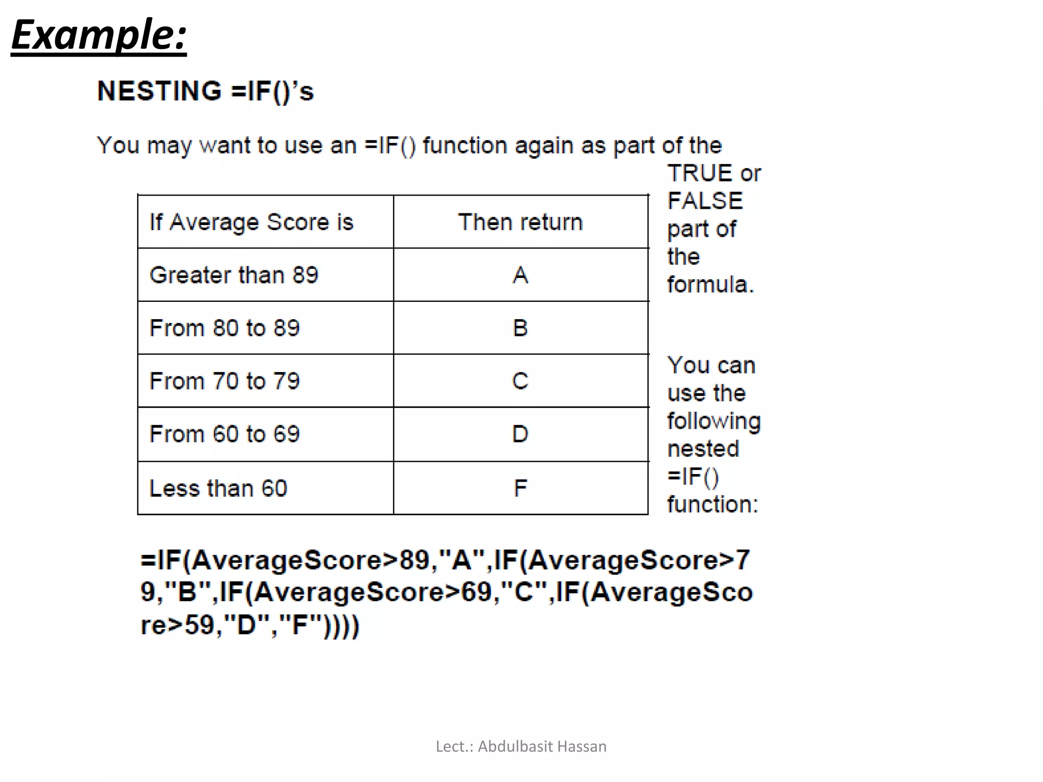
115.
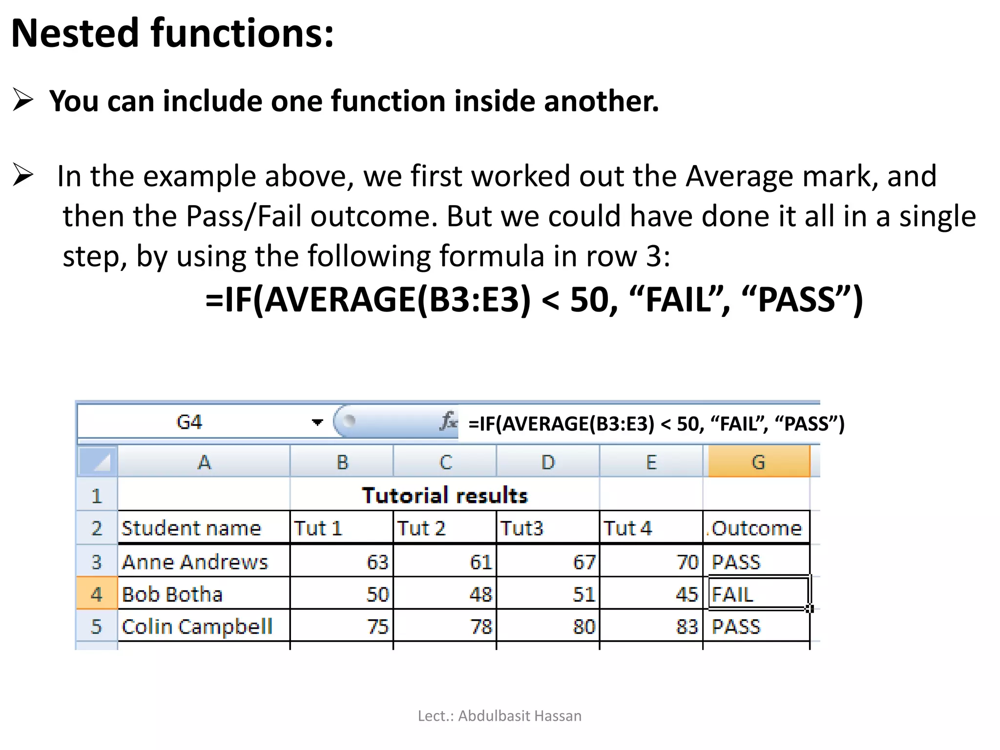
You caninclude one function inside another.
Nested functions:
In the example above, we first worked out the Average mark, and
then the Pass/Fail outcome. But we could have done it all in a single
step, by using the following formula in row 3:
=IF(AVERAGE(B3:E3) < 50, “FAIL”, “PASS”)
=IF(AVERAGE(B3:E3) < 50, “FAIL”, “PASS”)
Lect.: Abdulbasit Hassan
116.
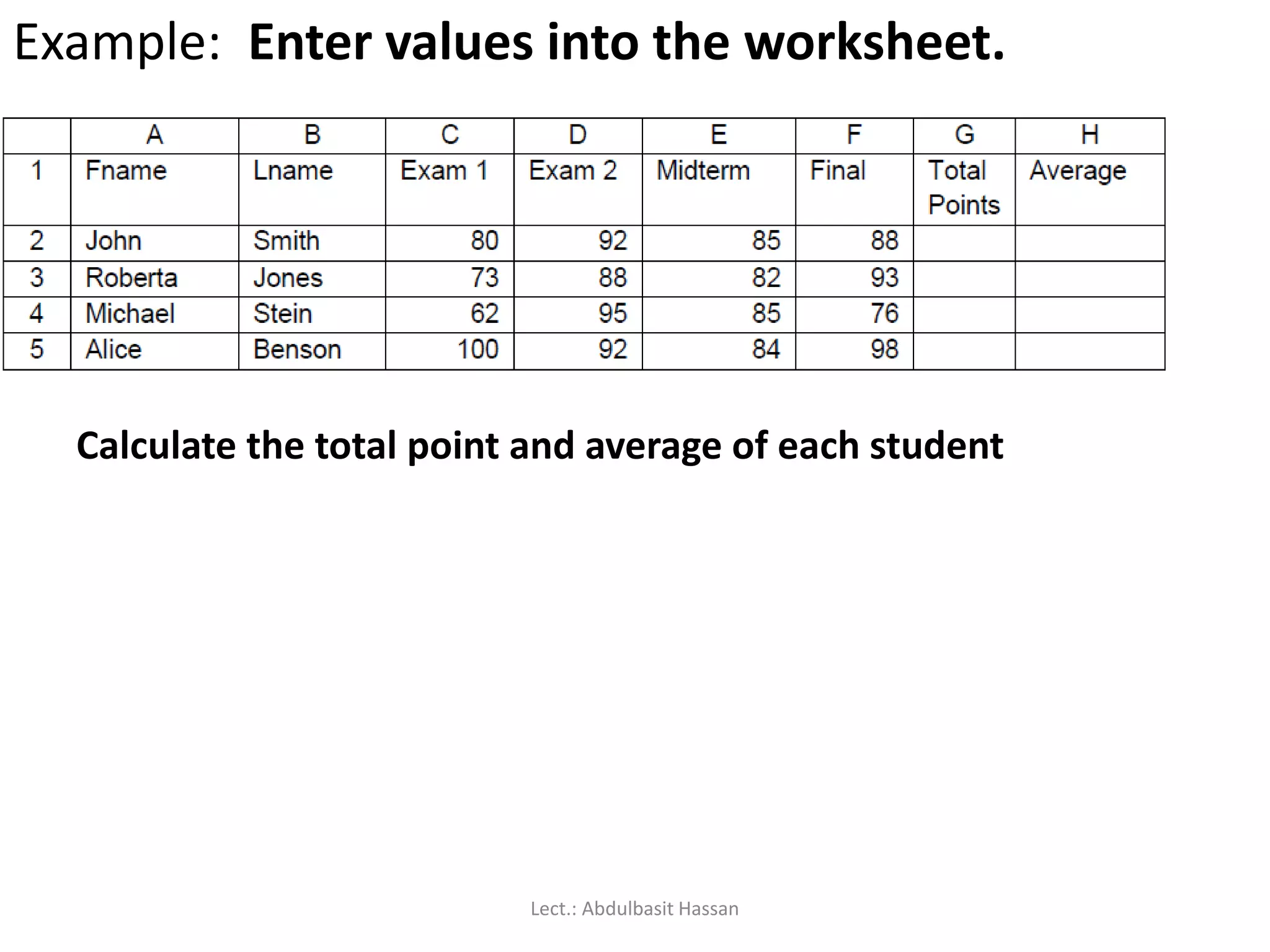
Example: Enter valuesinto the worksheet.
Calculate the total point and average of each student
Lect.: Abdulbasit Hassan
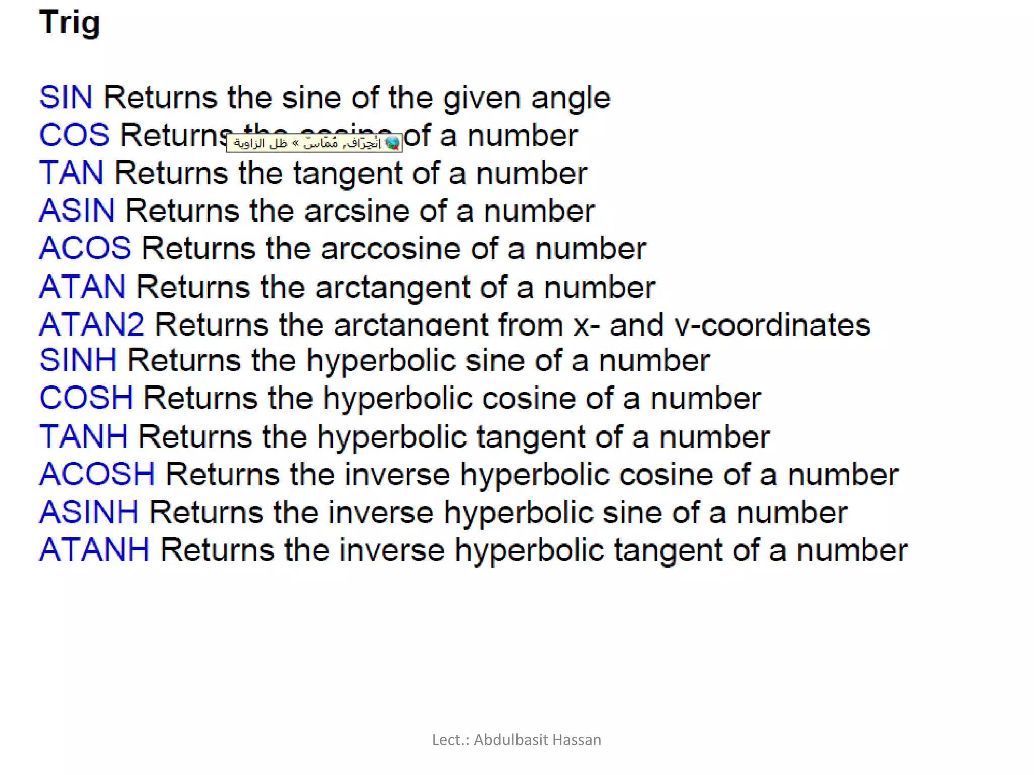
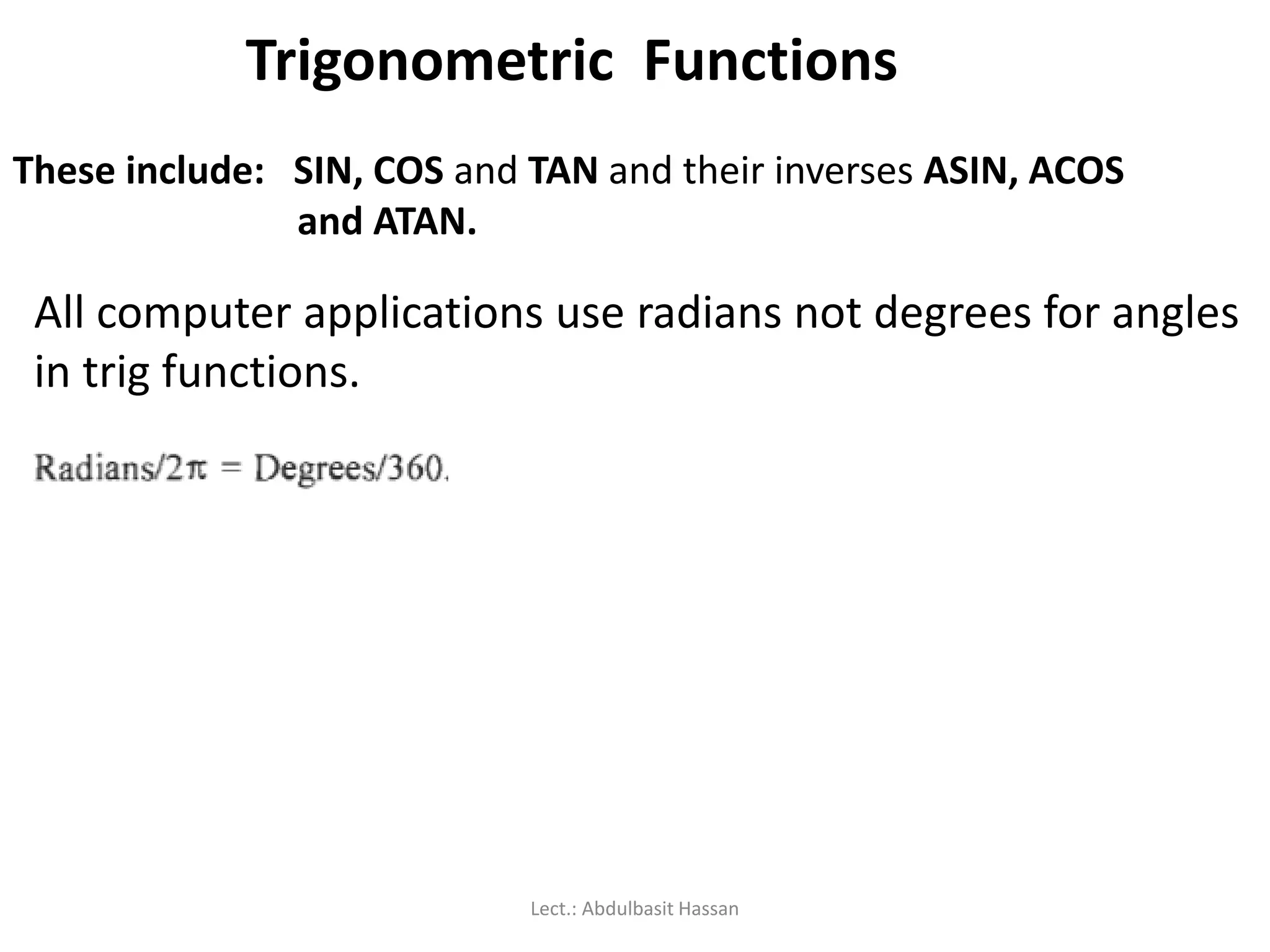
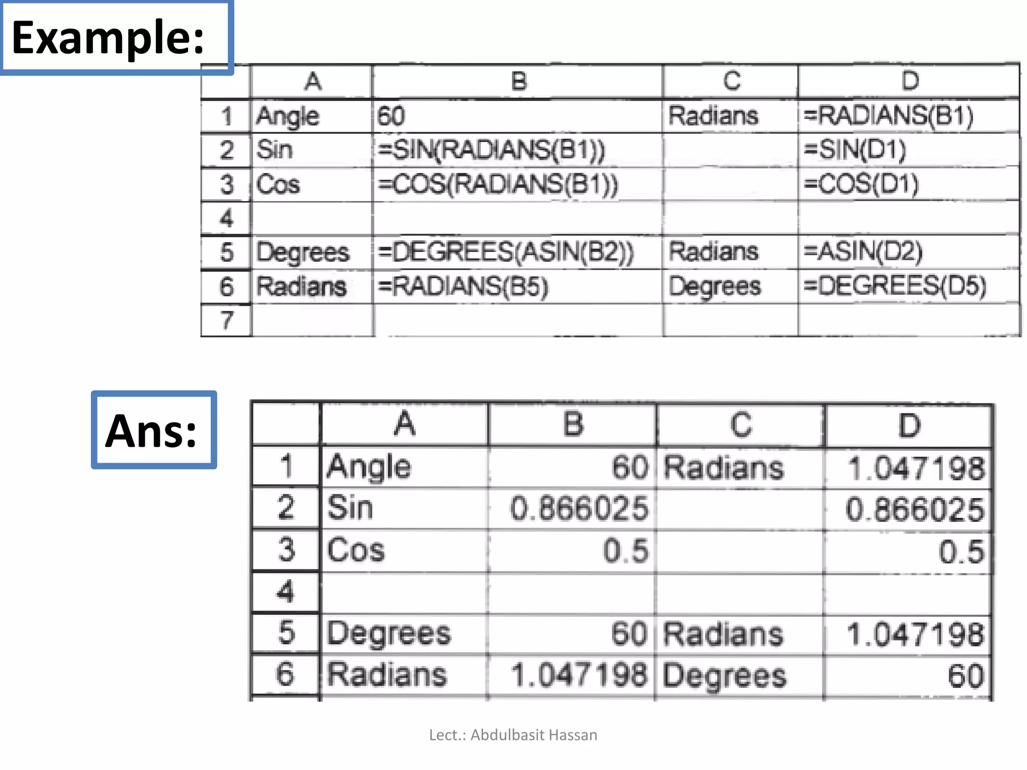
Trigonometric Functions
These include:SIN, COS and TAN and their inverses ASIN, ACOS
and ATAN.
All computer applications use radians not degrees for angles
in trig functions.
Lect.: Abdulbasit Hassan
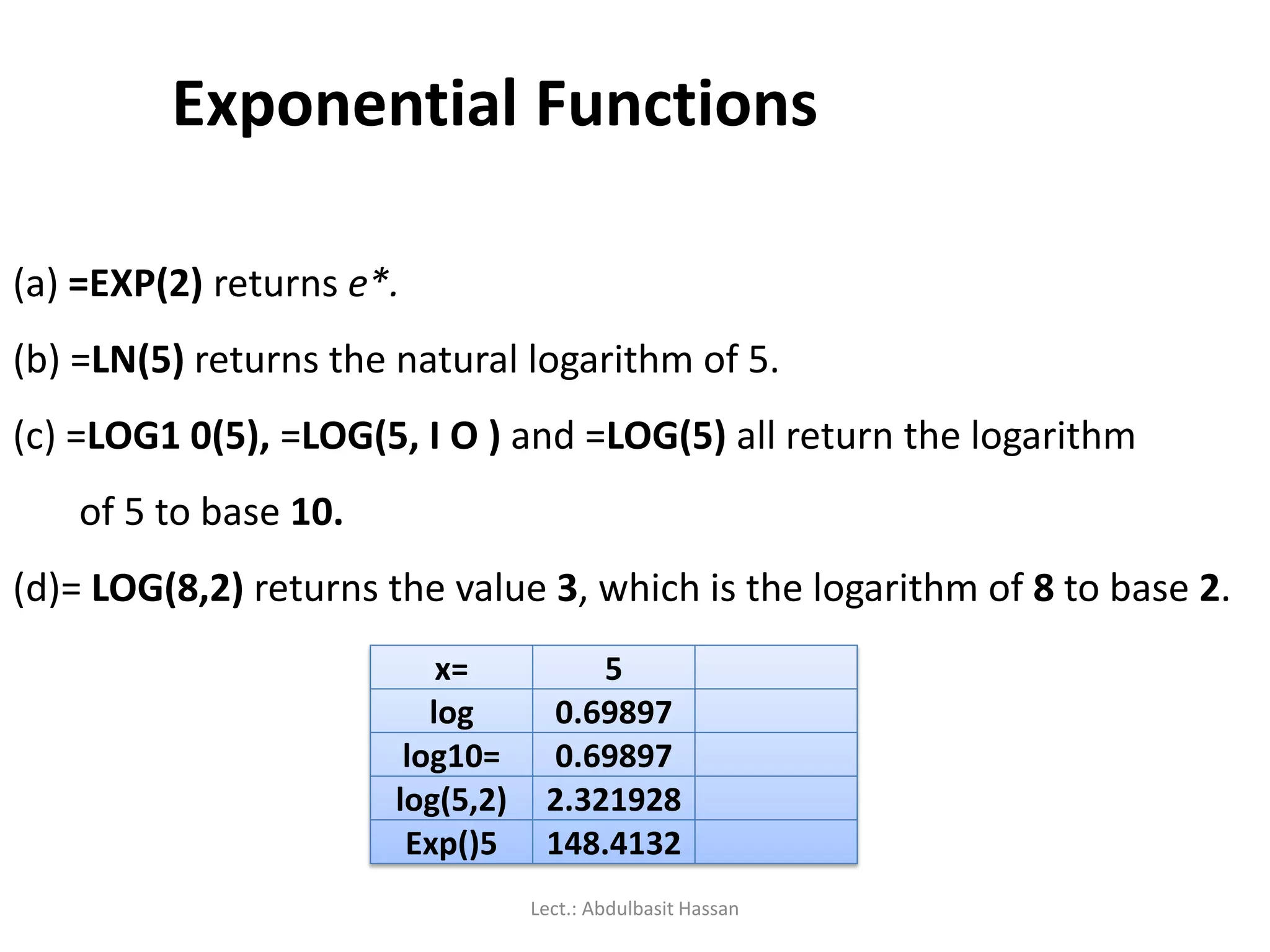
Exponential Functions
(a) =EXP(2)returns e*.
(b) =LN(5) returns the natural logarithm of 5.
(c) =LOG1 0(5), =LOG(5, I O ) and =LOG(5) all return the logarithm
of 5 to base 10.
(d)= LOG(8,2) returns the value 3, which is the logarithm of 8 to base 2.
x= 5
log 0.69897
log10= 0.69897
log(5,2) 2.321928
Exp()5 148.4132
Lect.: Abdulbasit Hassan
125.
Rounding Function
Excel providesa number of functions which
either truncate or round a value to a required
number of digits or to a multiple of some
number.
Lect.: Abdulbasit Hassan
A number oferrors can arise with formulas and
functions. When this happens, Excel displays one of
these error values. See next slid.
Lect.: Abdulbasit Hassan
131.
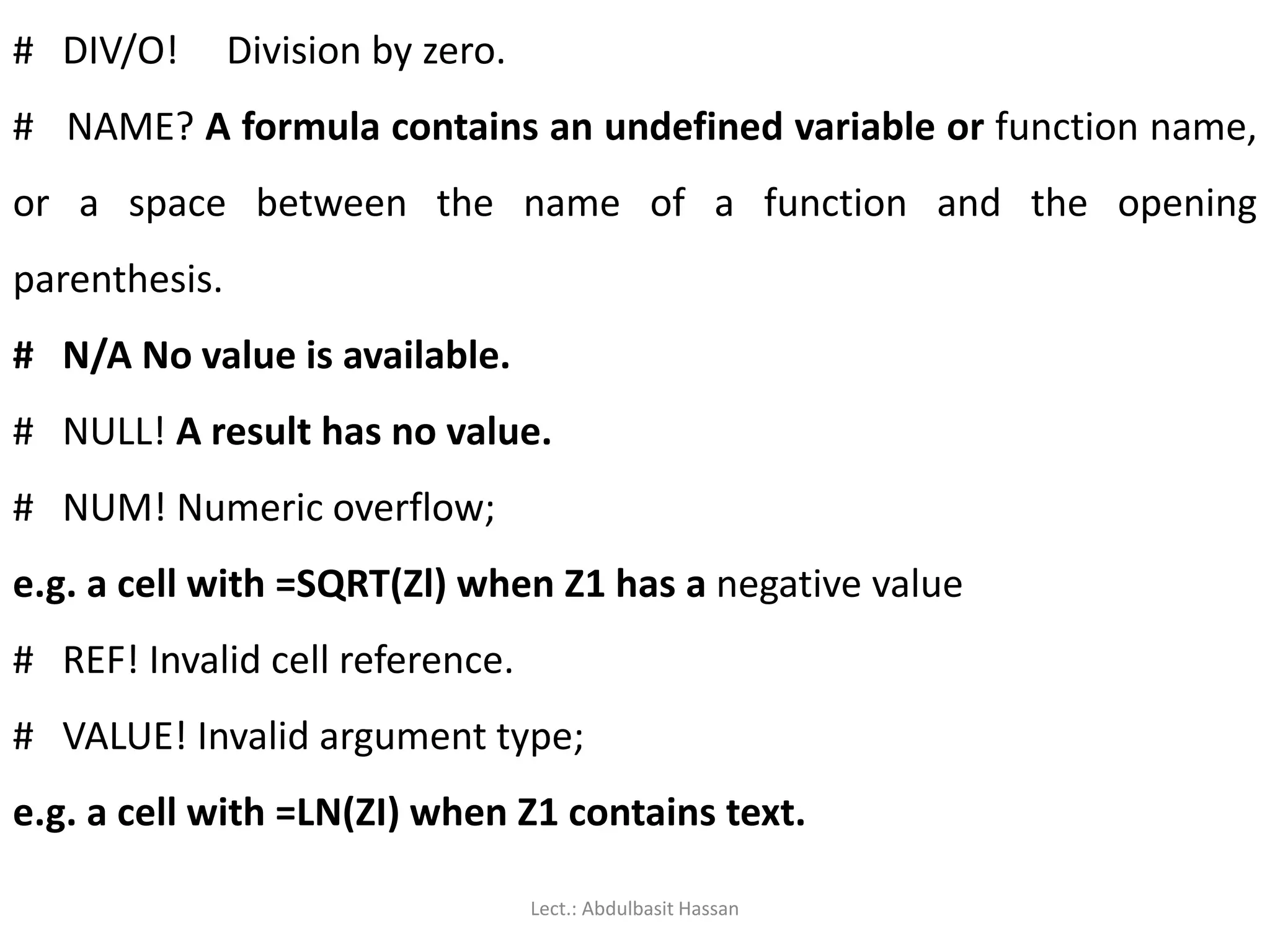
# DIV/O! Divisionby zero.
# NAME? A formula contains an undefined variable or function name,
or a space between the name of a function and the opening
parenthesis.
# N/A No value is available.
# NULL! A result has no value.
# NUM! Numeric overflow;
e.g. a cell with =SQRT(Zl) when Z1 has a negative value
# REF! Invalid cell reference.
# VALUE! Invalid argument type;
e.g. a cell with =LN(ZI) when Z1 contains text.
Lect.: Abdulbasit Hassan
To make Matrixoperations in Excel you must have in mind
that:
-Instead of using the ENTER (Return) key, you have to use the
CTRL-Shift-ENTER keys simultaneously. Excel uses this
command to know that we are making MATRIX operations.
Lect.: Abdulbasit Hassan
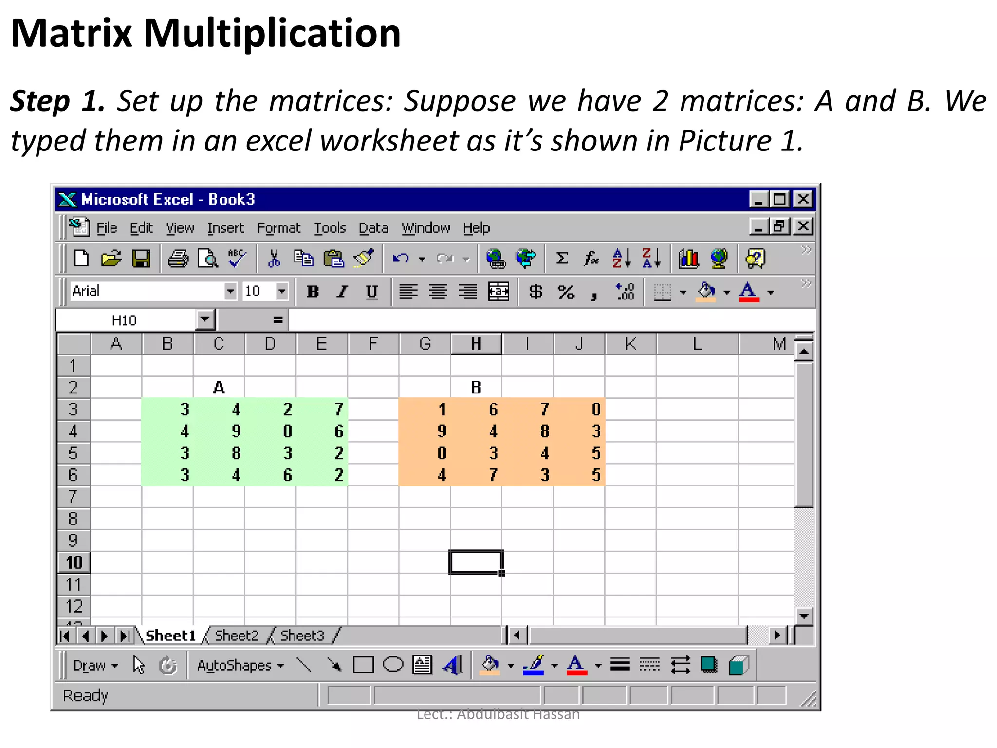
Matrix Multiplication
Step 1.Set up the matrices: Suppose we have 2 matrices: A and B. We
typed them in an excel worksheet as it’s shown in Picture 1.
Lect.: Abdulbasit Hassan
136.
Step 2. Wewant to Multiply A*B, then with the mouse (or
keyboard) “paint” the cells where the A*B matrix will be
placed. (Note that you must know the dimension of the new
matrix). In our example the A*B matrix will be 4*4 (since A is
4*4 and B is also 4*4), then we “paint” with the mouse a 4*4
matrix for the multiply output as shown in the picture 2.
Lect.: Abdulbasit Hassan
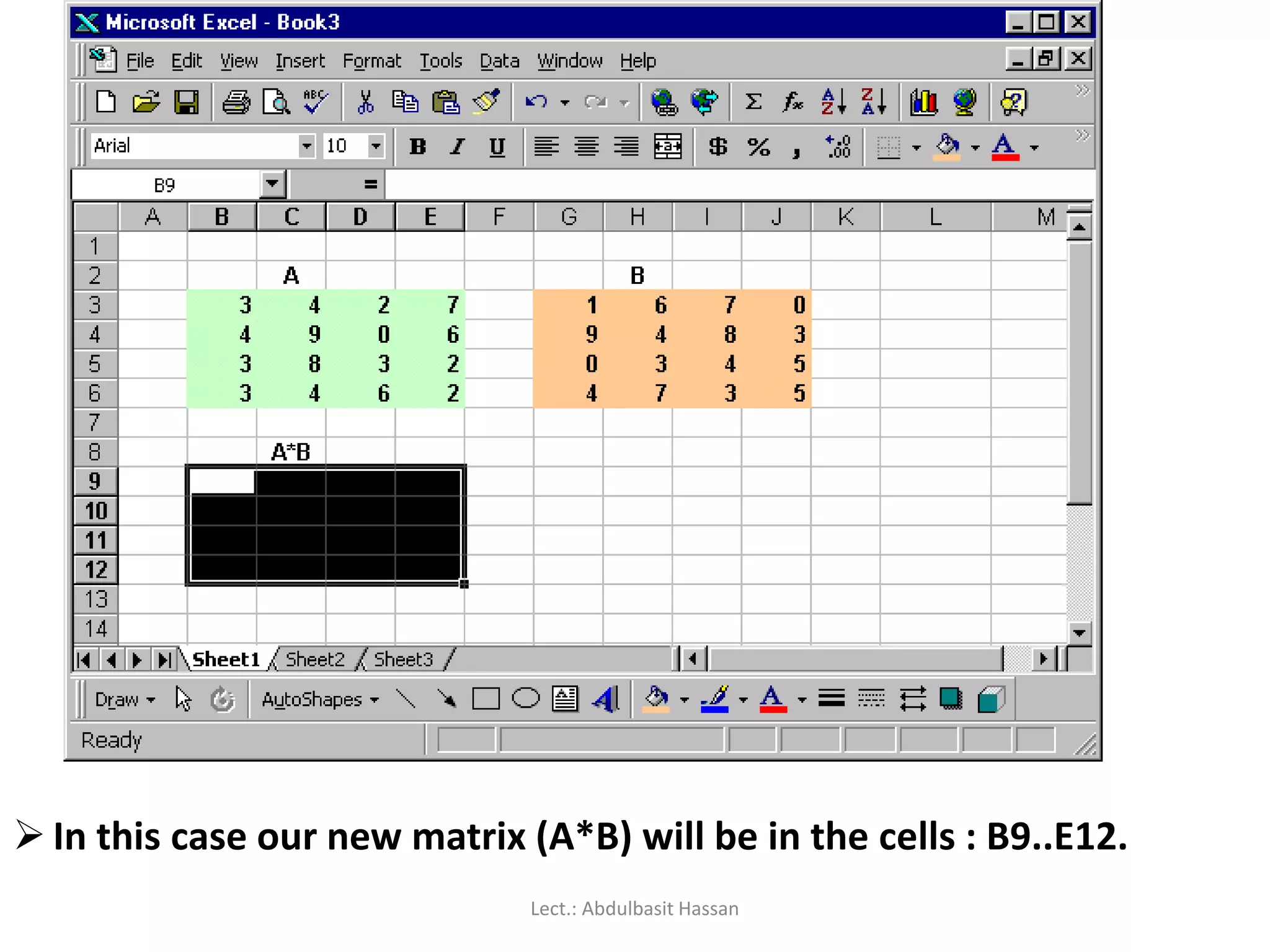
137.
In thiscase our new matrix (A*B) will be in the cells : B9..E12.
Lect.: Abdulbasit Hassan
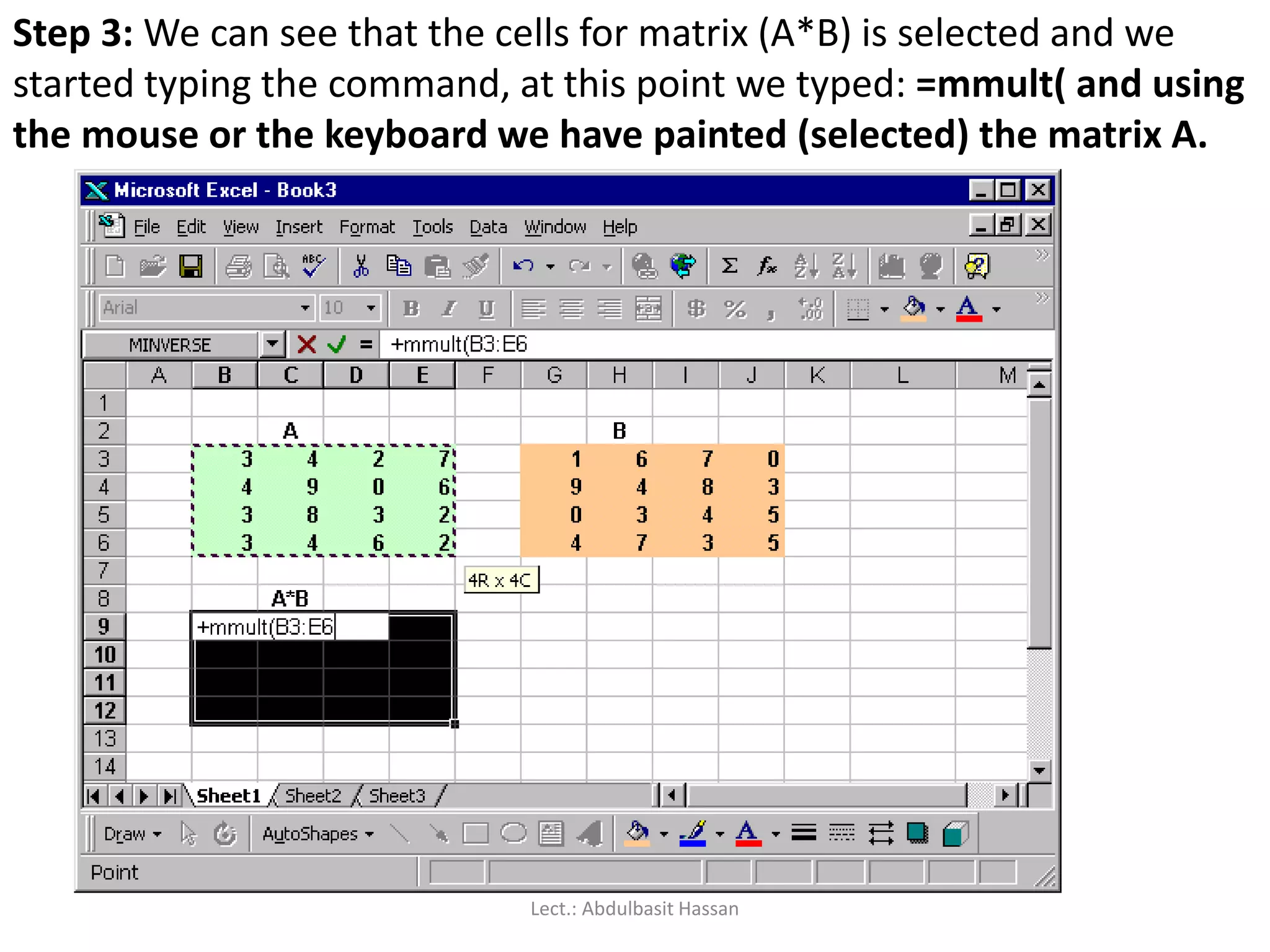
138.
Step 3: Wecan see that the cells for matrix (A*B) is selected and we
started typing the command, at this point we typed: =mmult( and using
the mouse or the keyboard we have painted (selected) the matrix A.
Lect.: Abdulbasit Hassan
139.
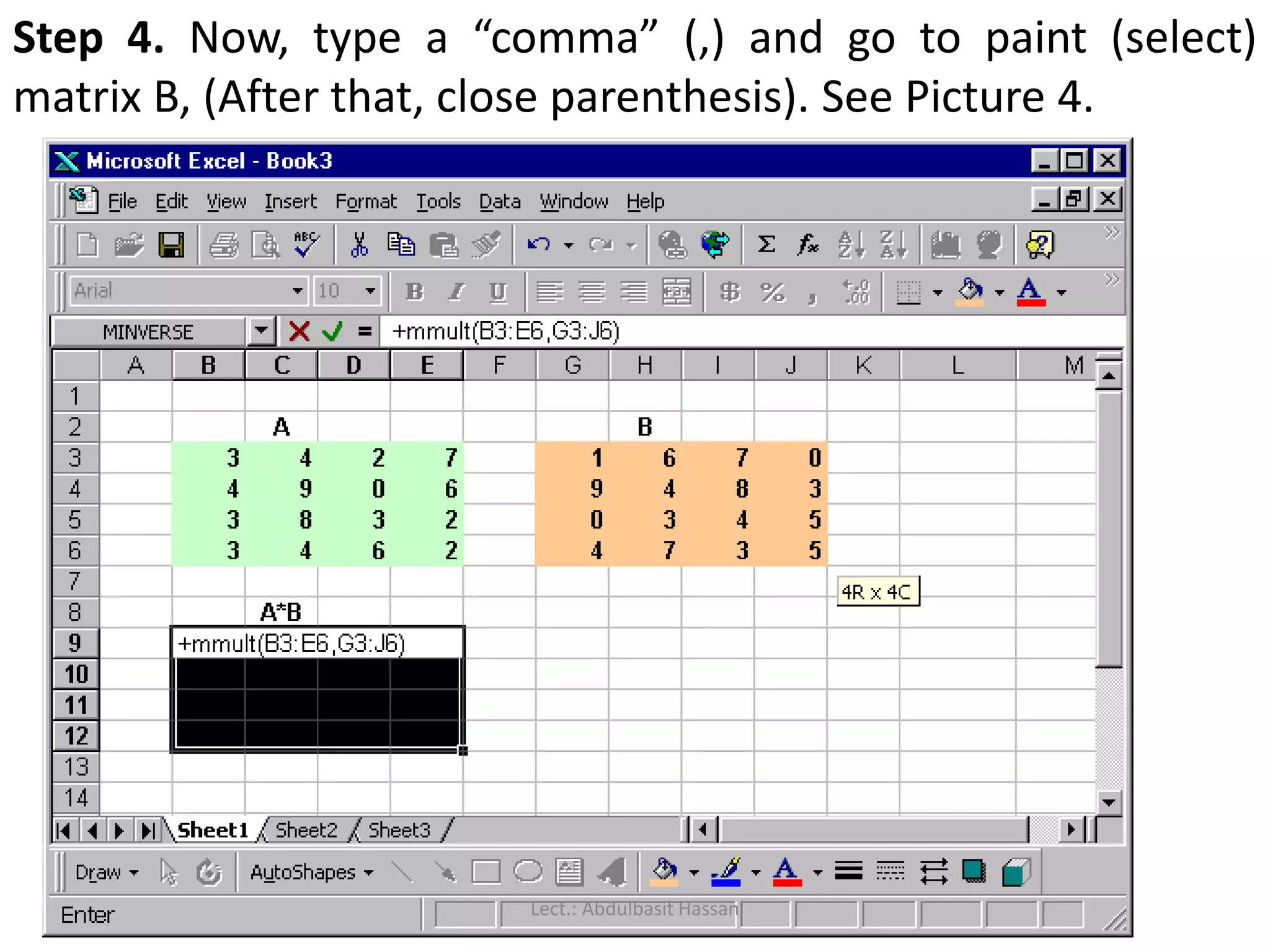
Step 4. Now,type a “comma” (,) and go to paint (select)
matrix B, (After that, close parenthesis). See Picture 4.
Lect.: Abdulbasit Hassan
140.
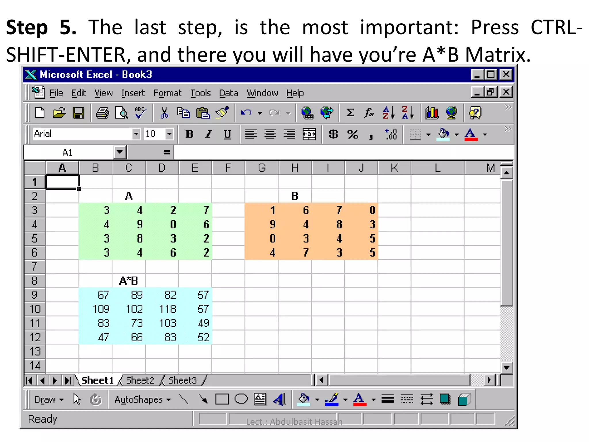
Step 5. Thelast step, is the most important: Press CTRL-
SHIFT-ENTER, and there you will have you’re A*B Matrix.
Lect.: Abdulbasit Hassan
141.
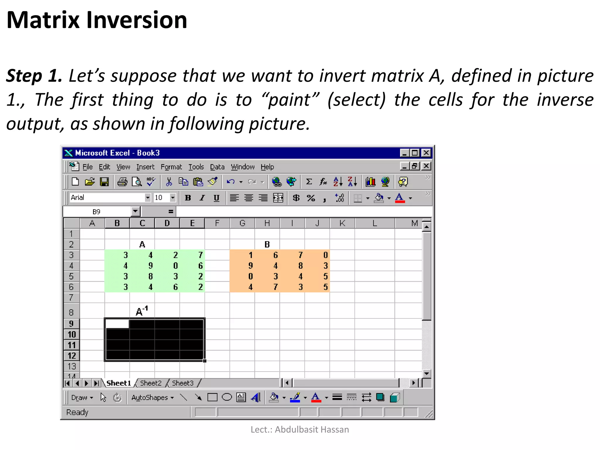
Matrix Inversion
Step 1.Let’s suppose that we want to invert matrix A, defined in picture
1., The first thing to do is to “paint” (select) the cells for the inverse
output, as shown in following picture.
Lect.: Abdulbasit Hassan
142.
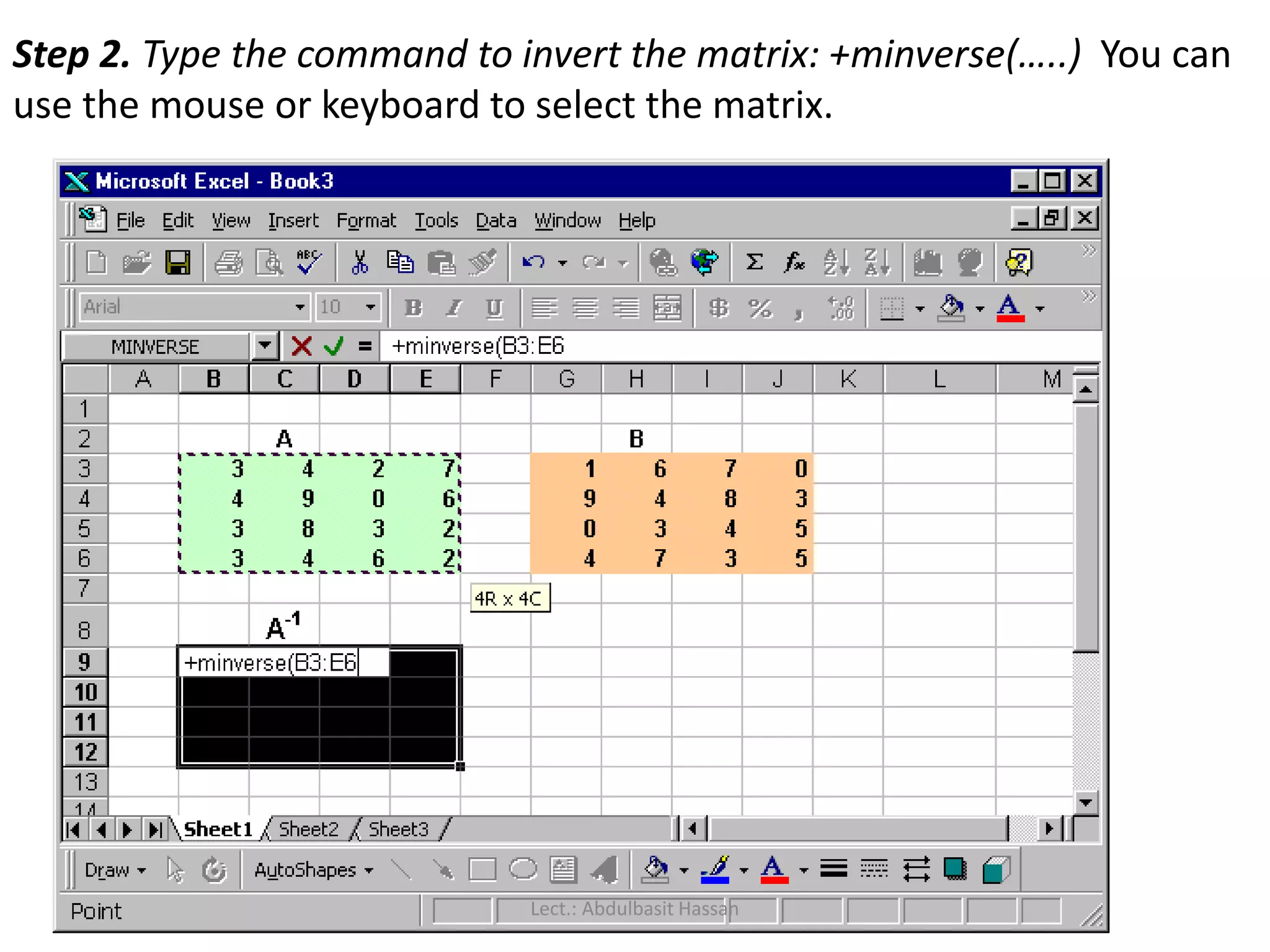
Step 2. Typethe command to invert the matrix: +minverse(…..) You can
use the mouse or keyboard to select the matrix.
Lect.: Abdulbasit Hassan
143.
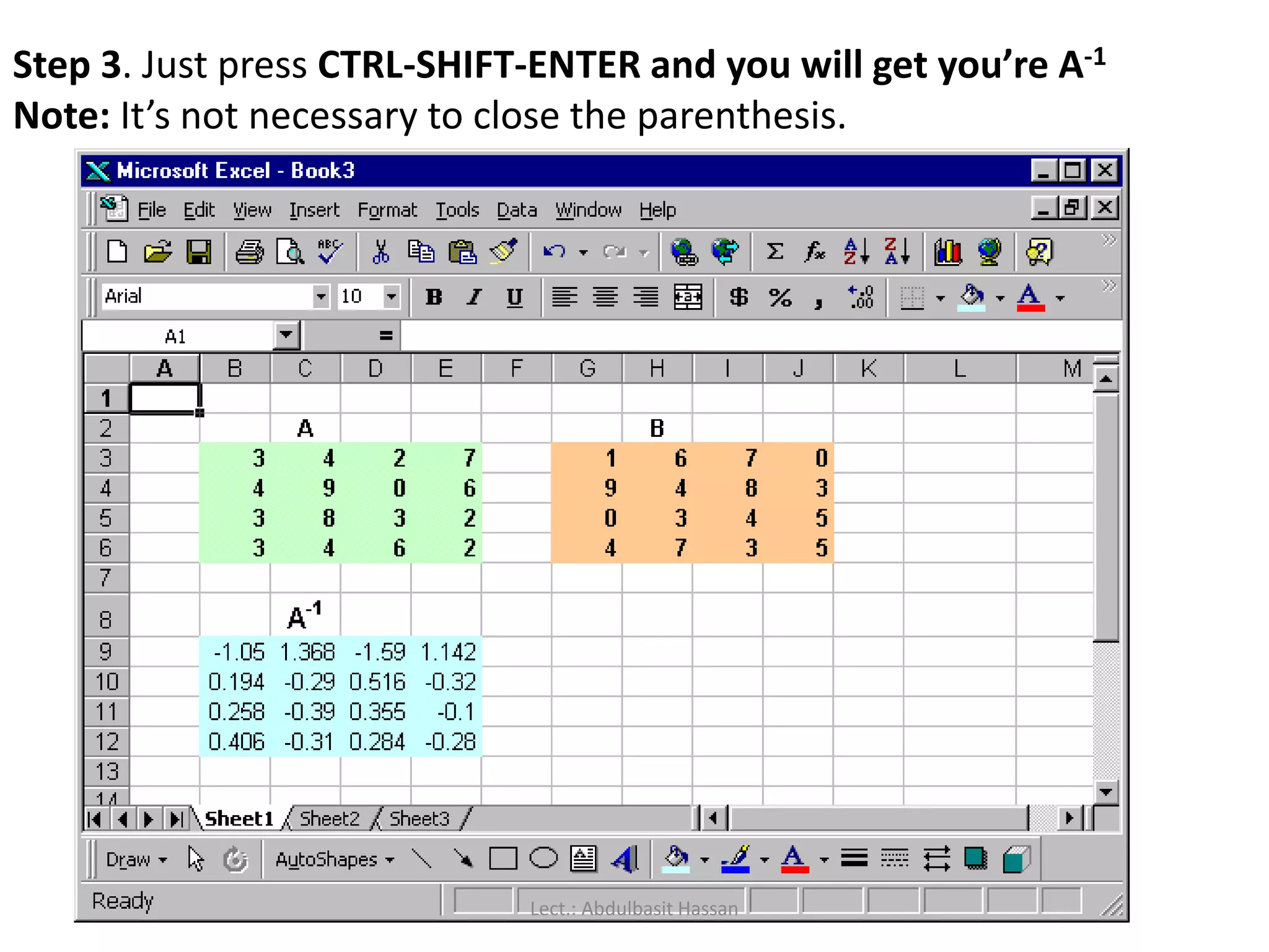
Step 3. Justpress CTRL-SHIFT-ENTER and you will get you’re A-1
Note: It’s not necessary to close the parenthesis.
Lect.: Abdulbasit Hassan
144.
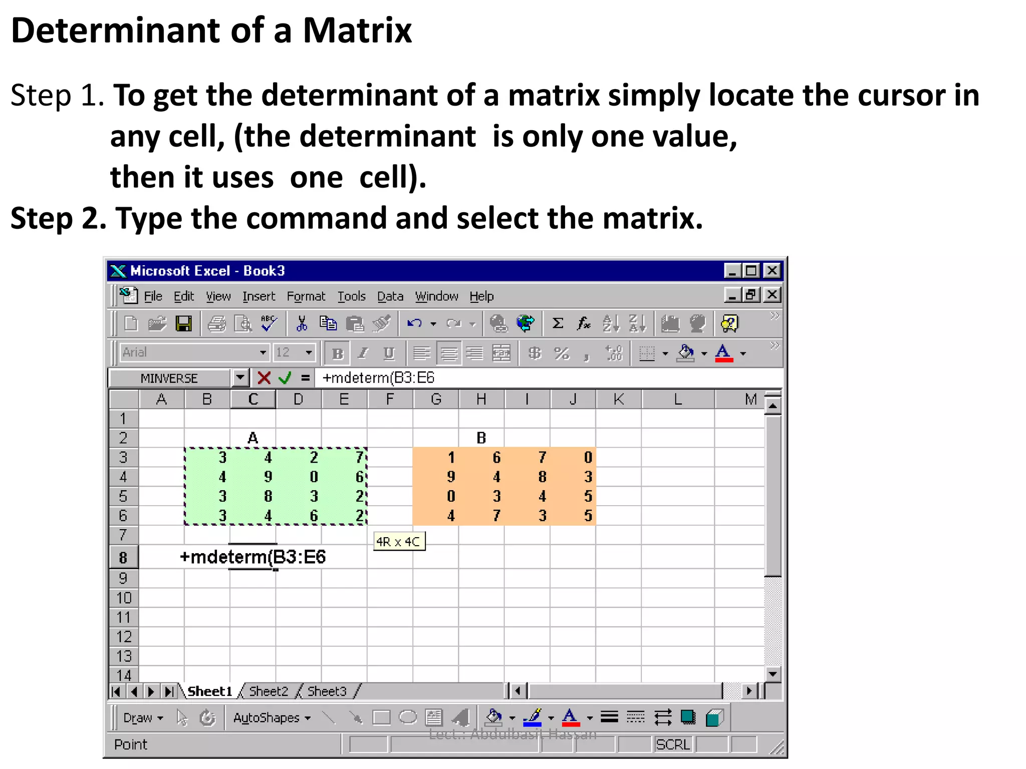
Determinant of aMatrix
Step 1. To get the determinant of a matrix simply locate the cursor in
any cell, (the determinant is only one value,
then it uses one cell).
Step 2. Type the command and select the matrix.
Lect.: Abdulbasit Hassan
145.
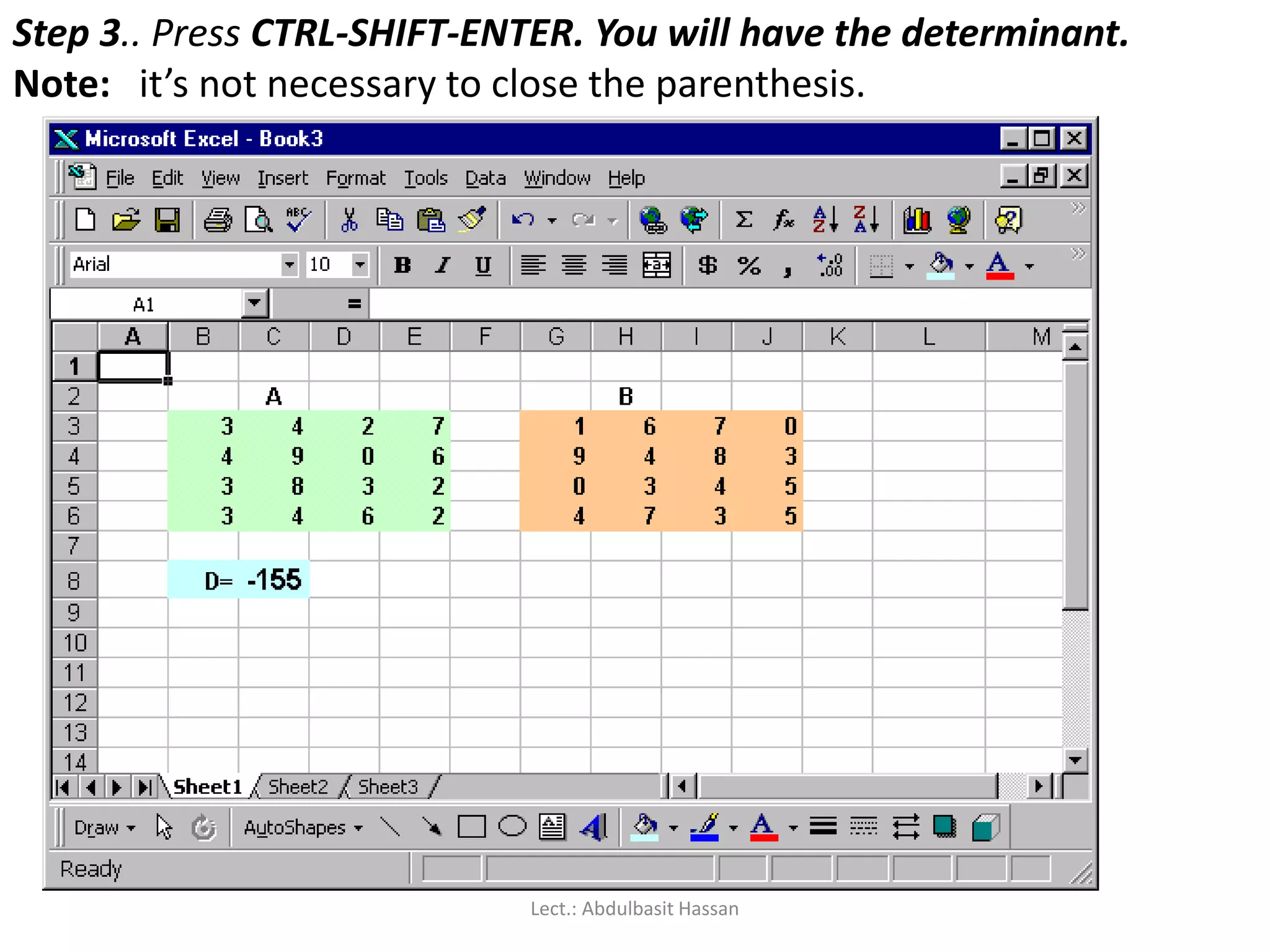
Step 3.. PressCTRL-SHIFT-ENTER. You will have the determinant.
Note: it’s not necessary to close the parenthesis.
Lect.: Abdulbasit Hassan
146.
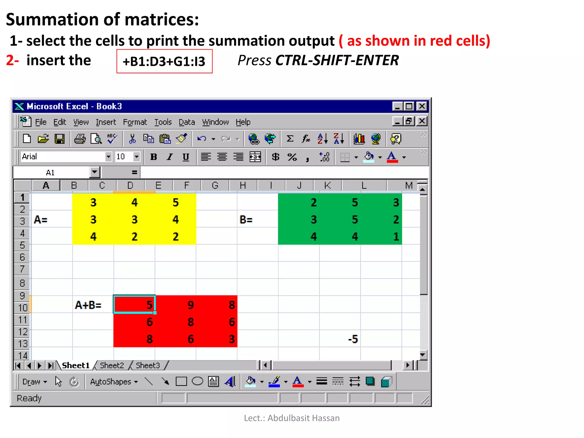
Summation of matrices:
1-select the cells to print the summation output ( as shown in red cells)
2- insert the Press CTRL-SHIFT-ENTER+B1:D3+G1:I3
Lect.: Abdulbasit Hassan
147.
A nonlinear programmingmodel consists
of a nonlinear objective function and
nonlinear constraints :
Lect.: Abdulbasit Hassan
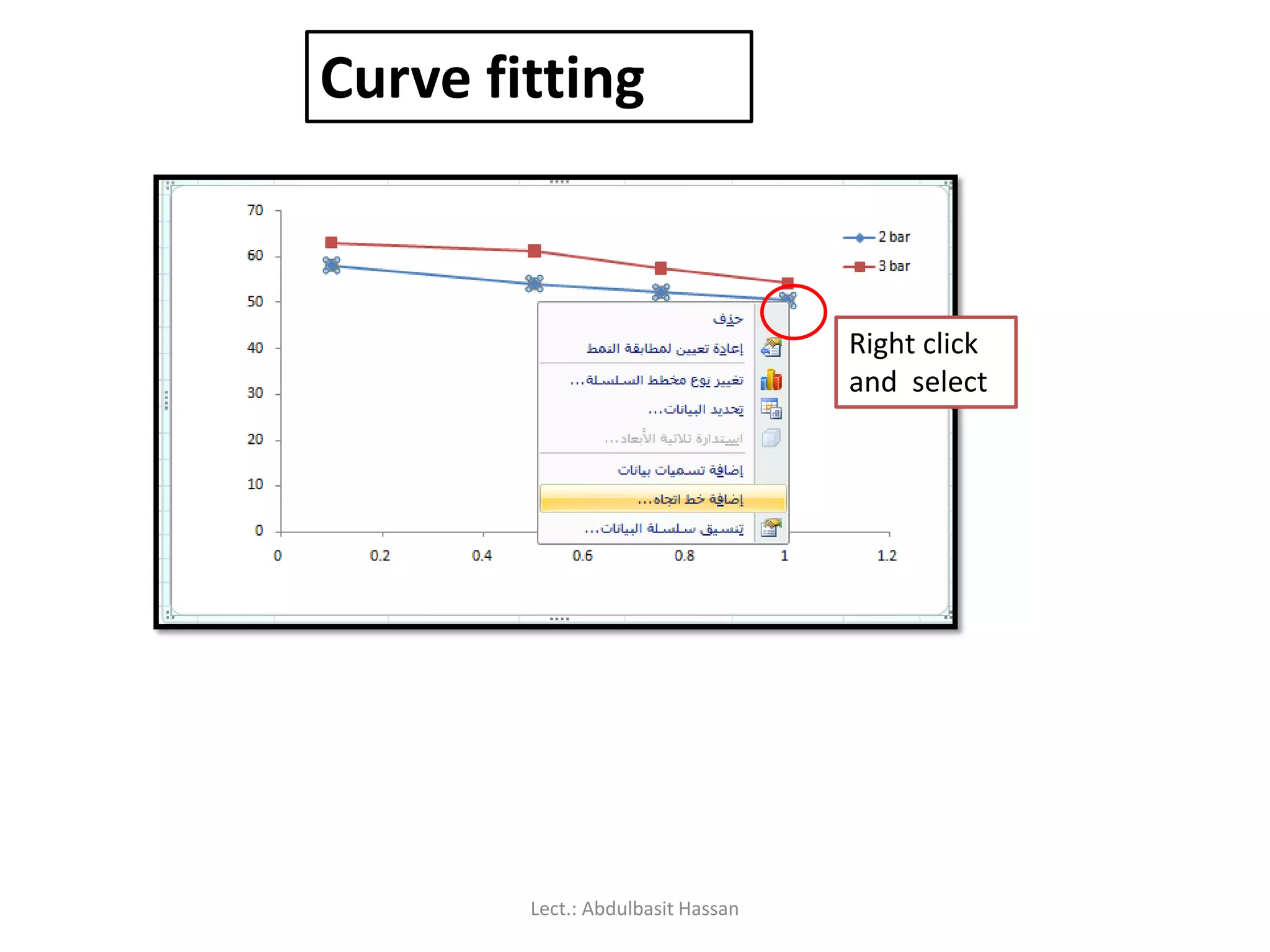
148.
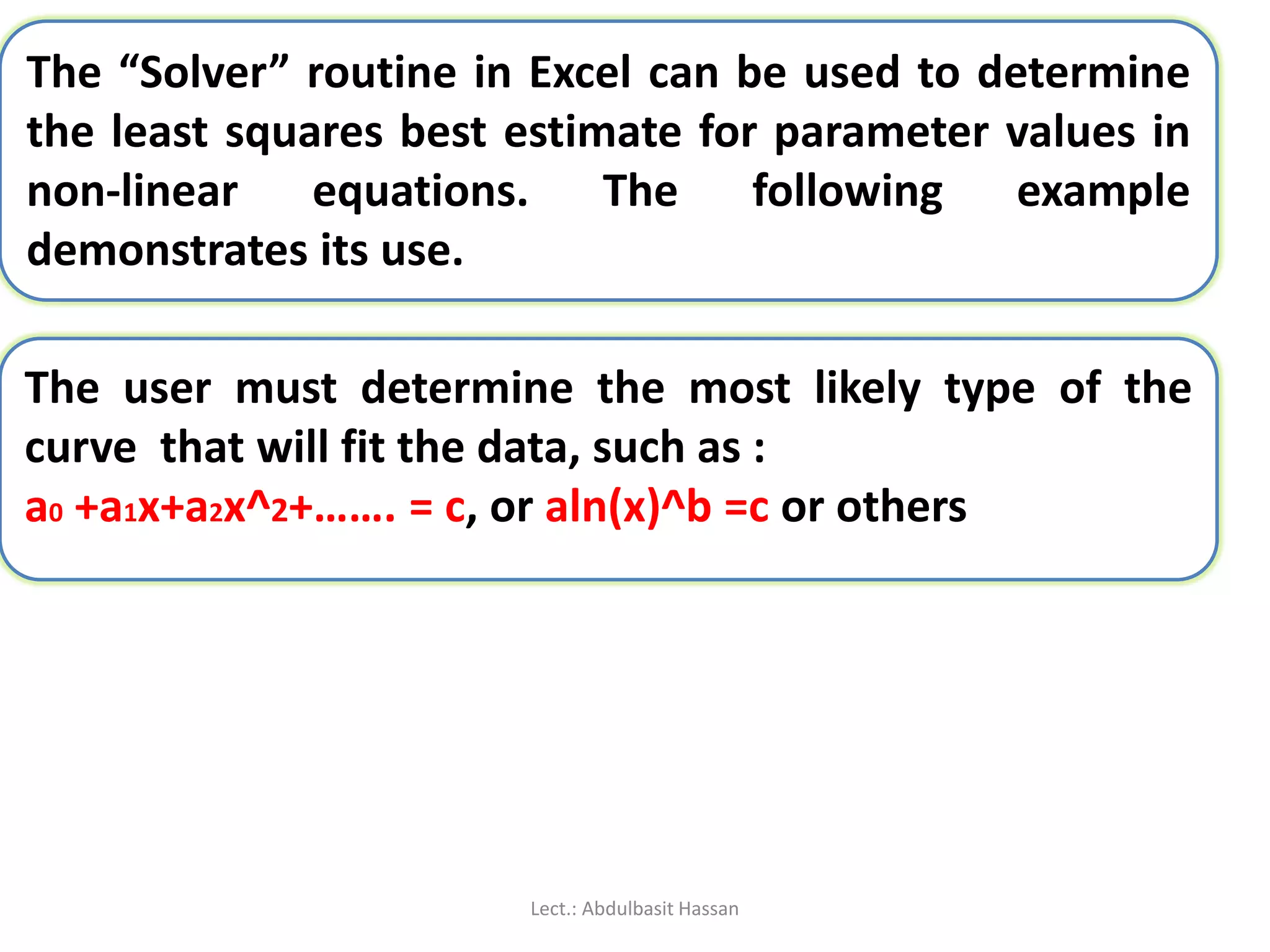
The “Solver” routinein Excel can be used to determine
the least squares best estimate for parameter values in
non-linear equations. The following example
demonstrates its use.
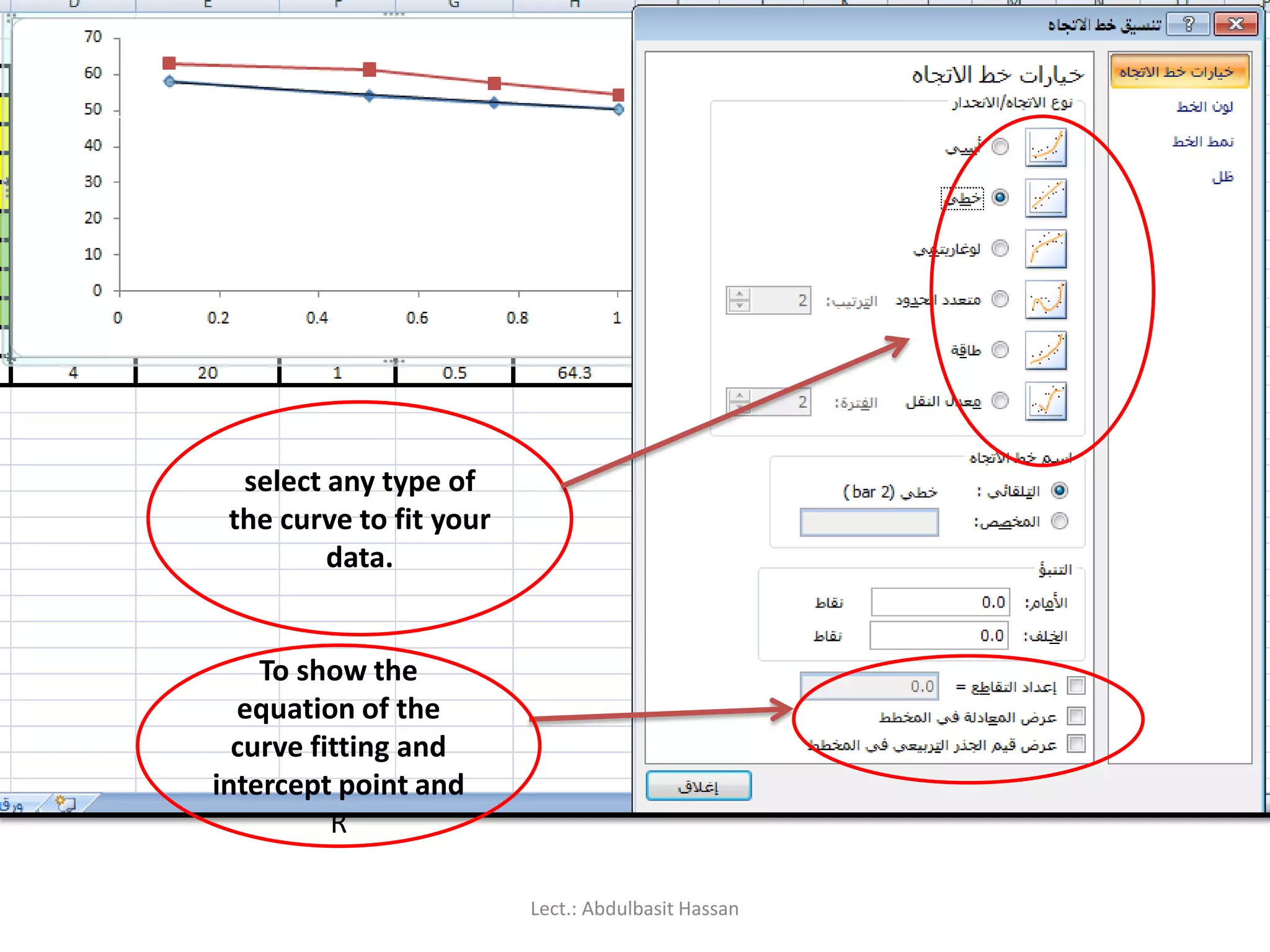
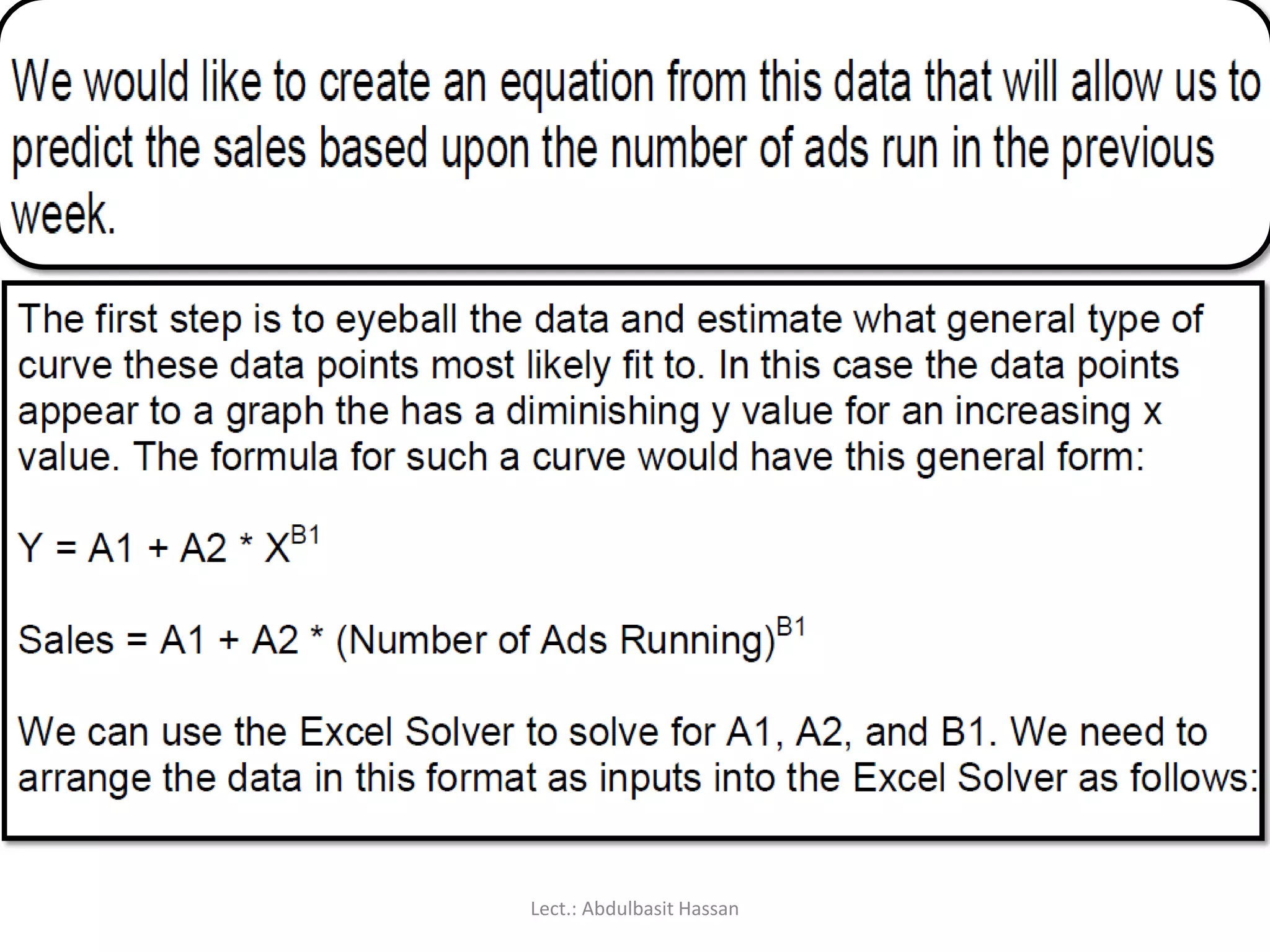
The user must determine the most likely type of the
curve that will fit the data, such as :
a0 +a1x+a2x^2+……. = c, or aln(x)^b =c or others
Lect.: Abdulbasit Hassan
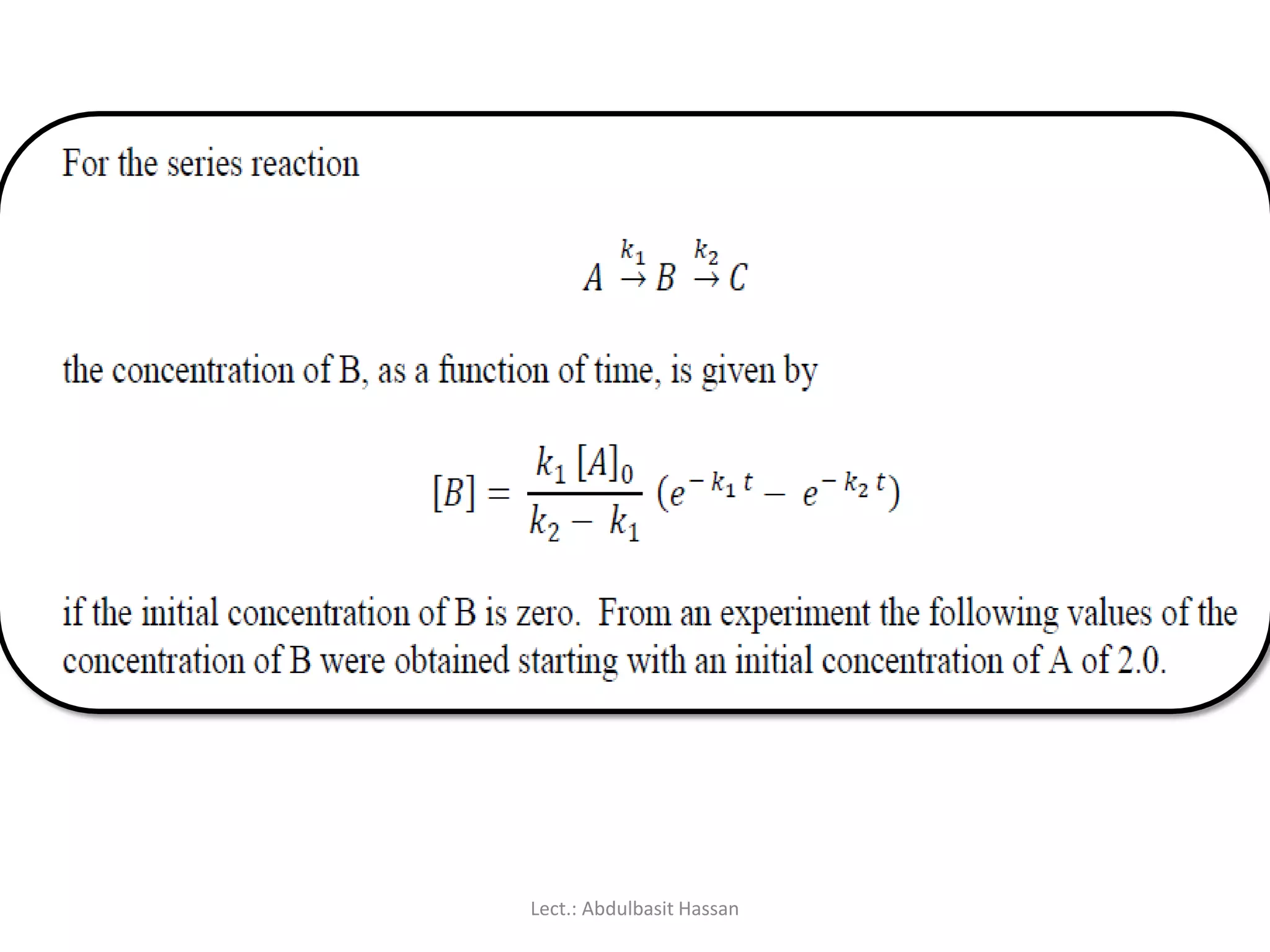
The task nowis to determine the best values for k1 and k2. However,
the expression of [B] is non-linear, and not easily transformed into a
linear form. We can, however, use “Solver” to accomplish the same
task.
Lect.: Abdulbasit Hassan
160.
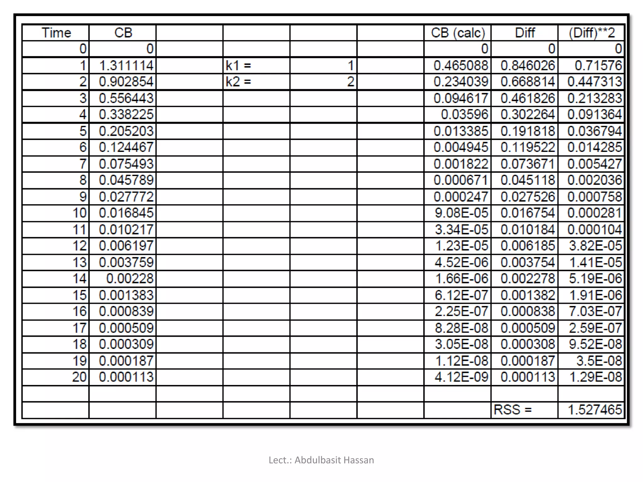
To start weneed to make initial estimates for both k1 and k2. Let’s
use 1 and 2. (Note: We don’t want to use the same value for both k1
and k2 since that would make the denominator term in the
expression for [B] zero.) With these two values we can use the
expression for [B] to calculate values for the concentration of B.
Lect.: Abdulbasit Hassan
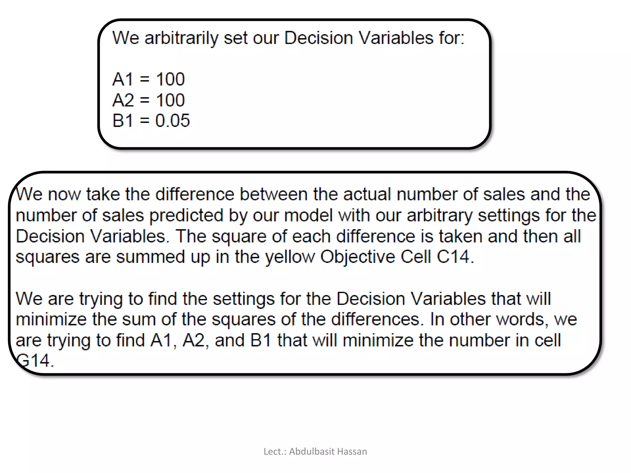
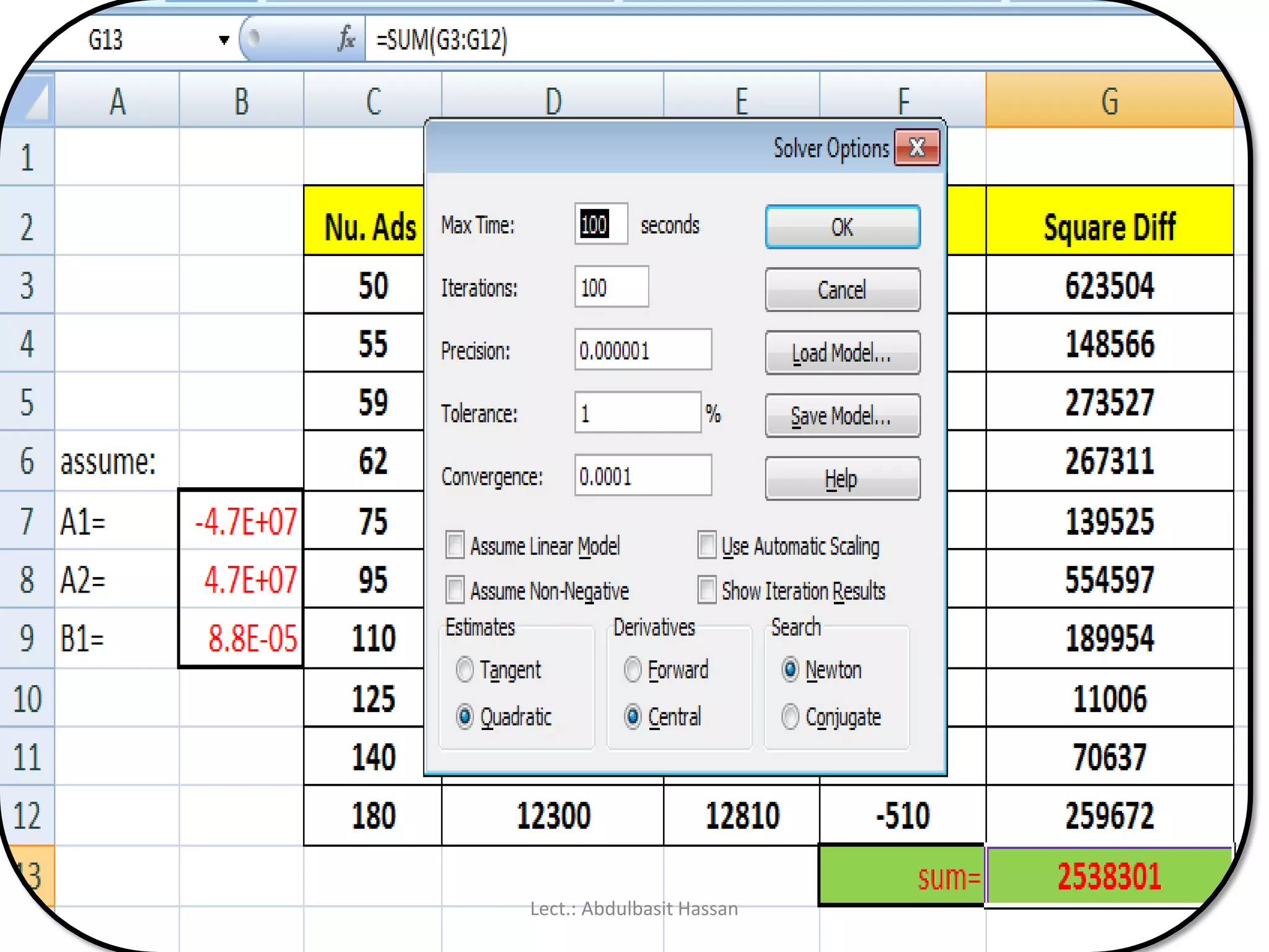
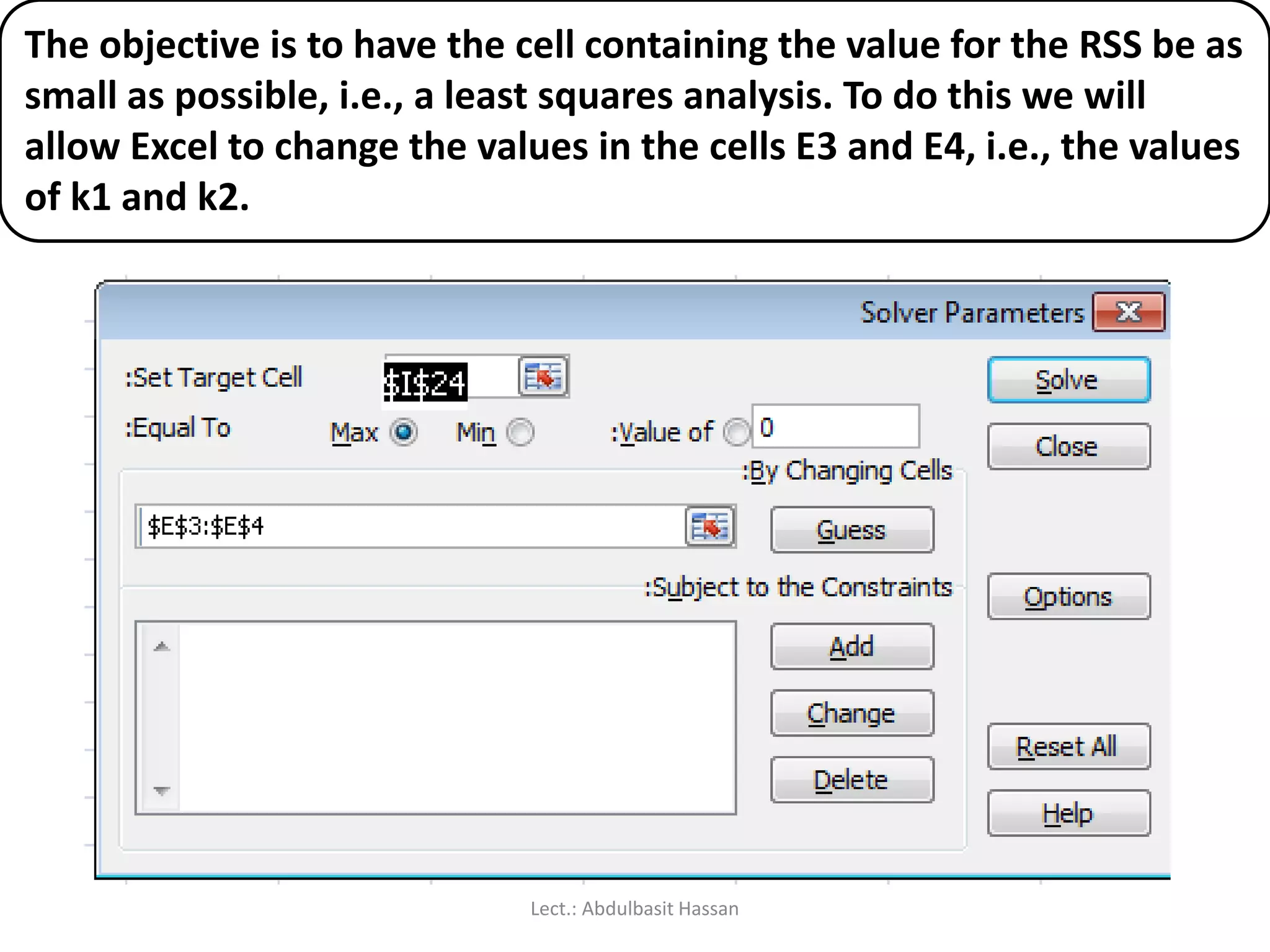
The objective isto have the cell containing the value for the RSS be as
small as possible, i.e., a least squares analysis. To do this we will
allow Excel to change the values in the cells E3 and E4, i.e., the values
of k1 and k2.
Lect.: Abdulbasit Hassan
163.
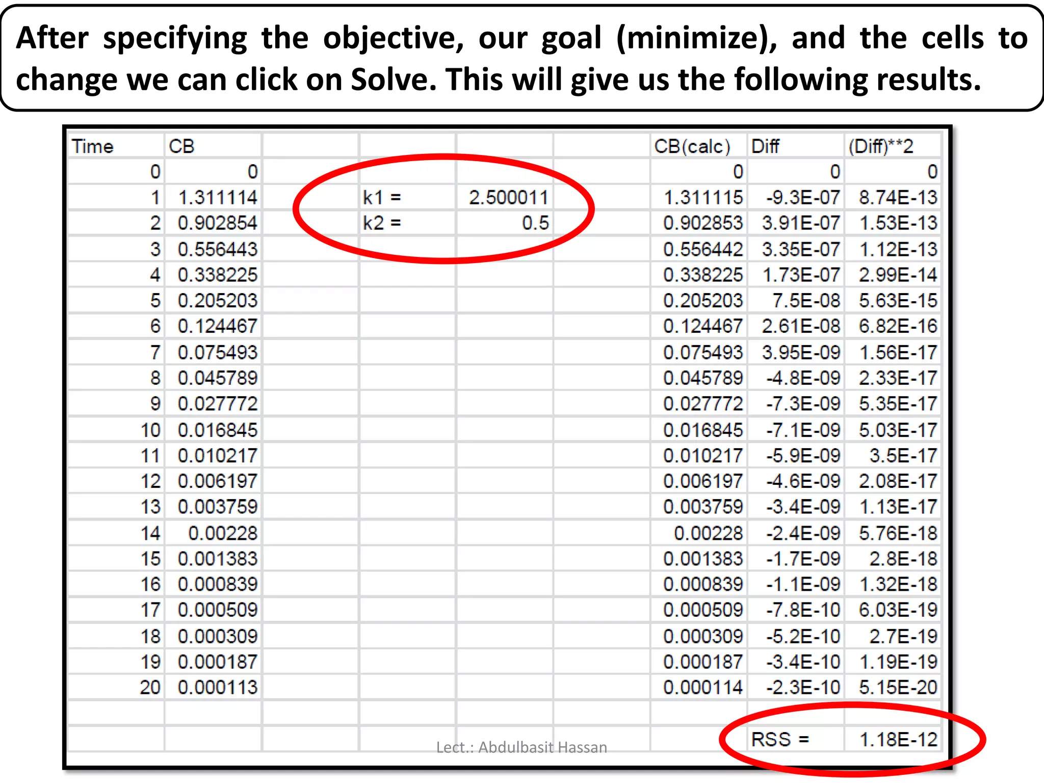
After specifying theobjective, our goal (minimize), and the cells to
change we can click on Solve. This will give us the following results.
Lect.: Abdulbasit Hassan
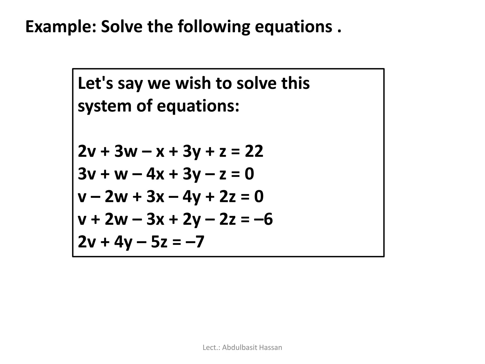
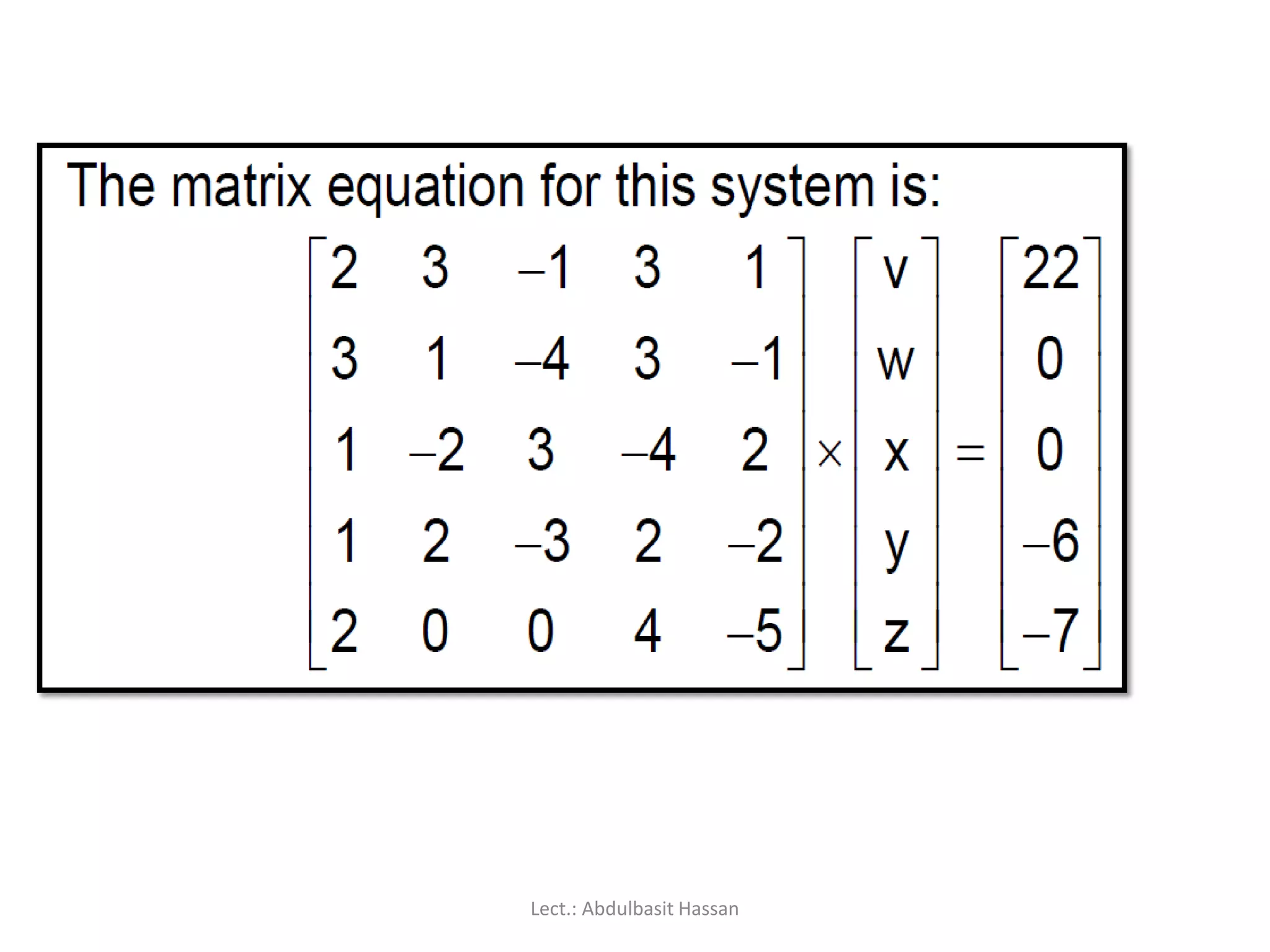
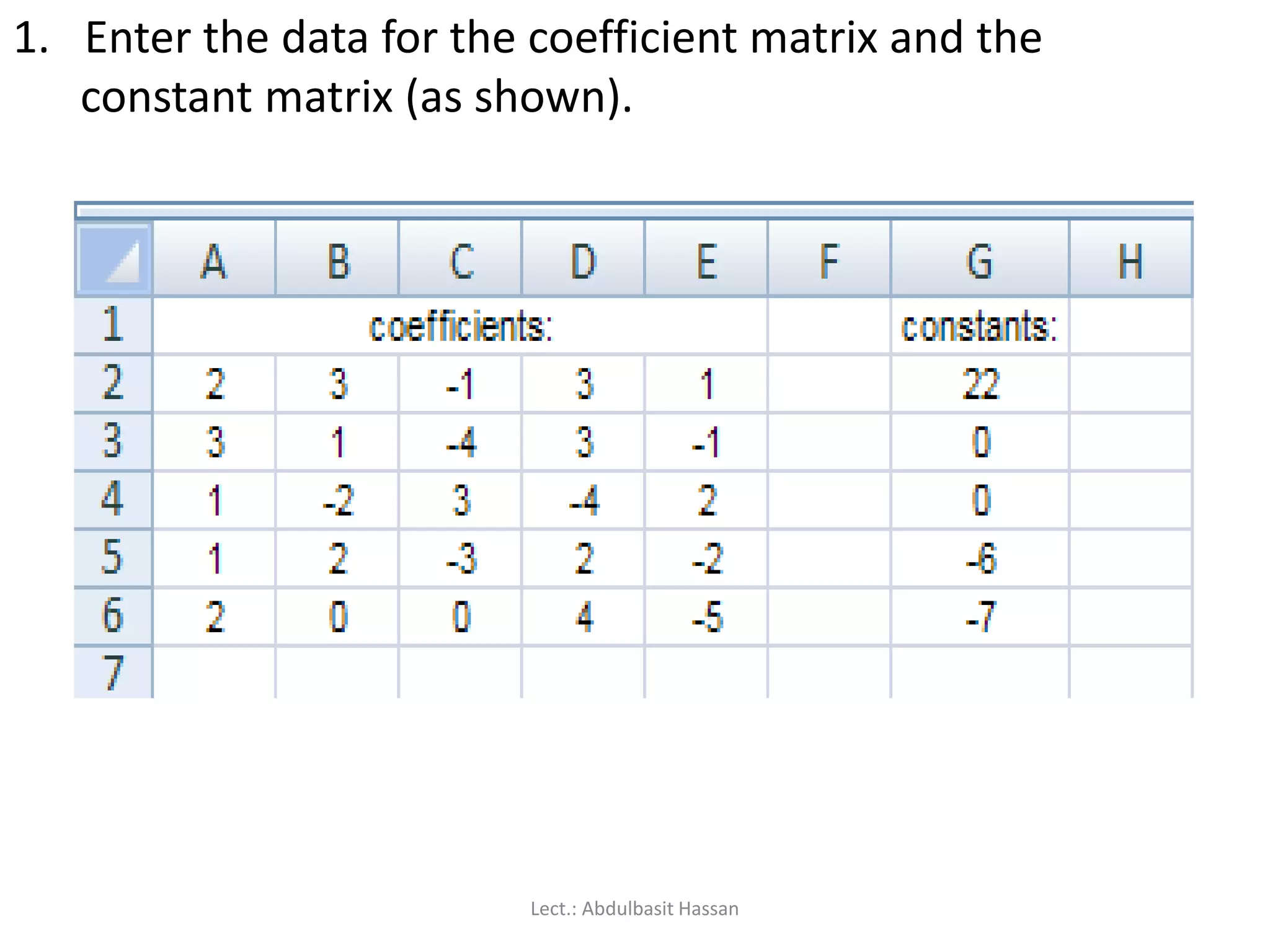
1. Enter thedata for the coefficient matrix and the
constant matrix (as shown).
Lect.: Abdulbasit Hassan
169.
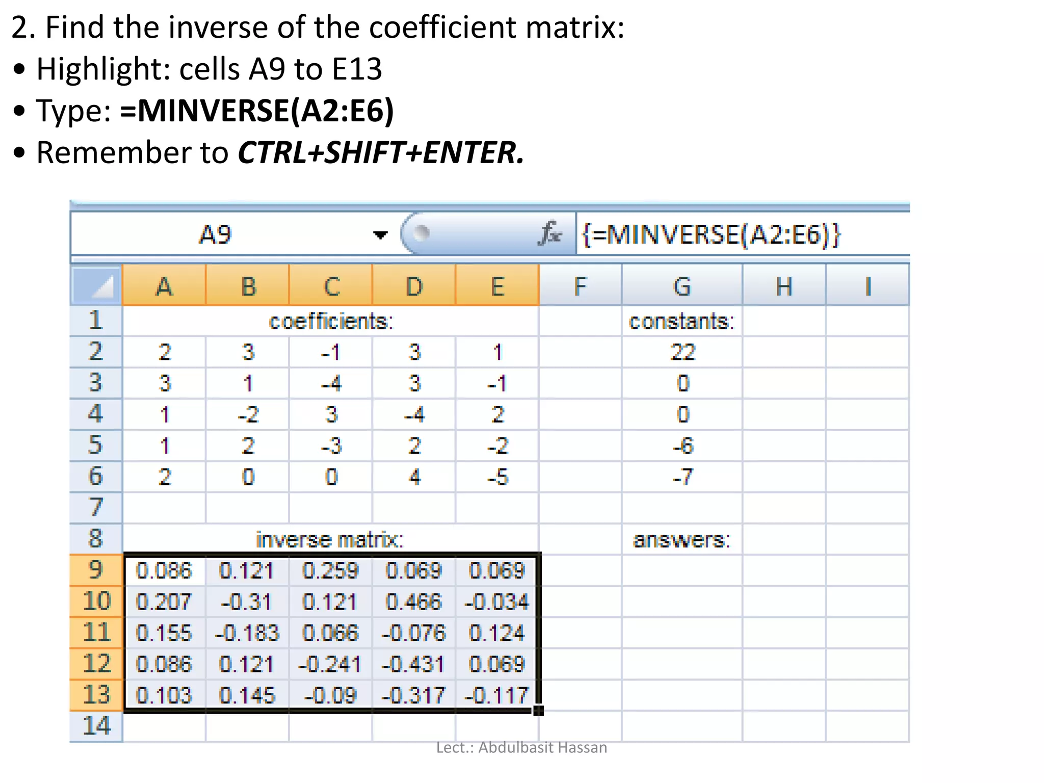
2. Find theinverse of the coefficient matrix:
• Highlight: cells A9 to E13
• Type: =MINVERSE(A2:E6)
• Remember to CTRL+SHIFT+ENTER.
Lect.: Abdulbasit Hassan
170.
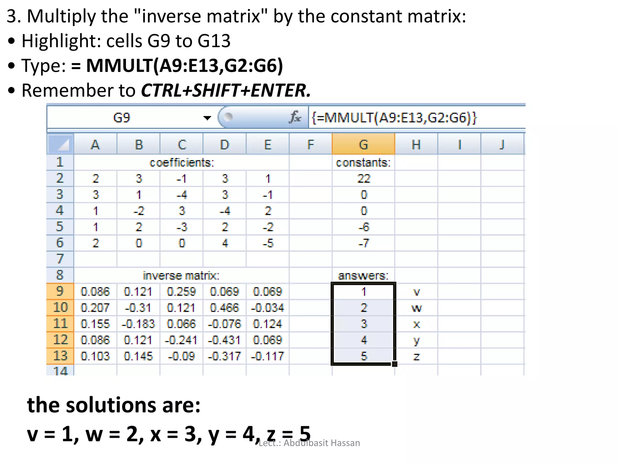
3. Multiply the"inverse matrix" by the constant matrix:
• Highlight: cells G9 to G13
• Type: = MMULT(A9:E13,G2:G6)
• Remember to CTRL+SHIFT+ENTER.
the solutions are:
v = 1, w = 2, x = 3, y = 4, z = 5Lect.: Abdulbasit Hassan
171.
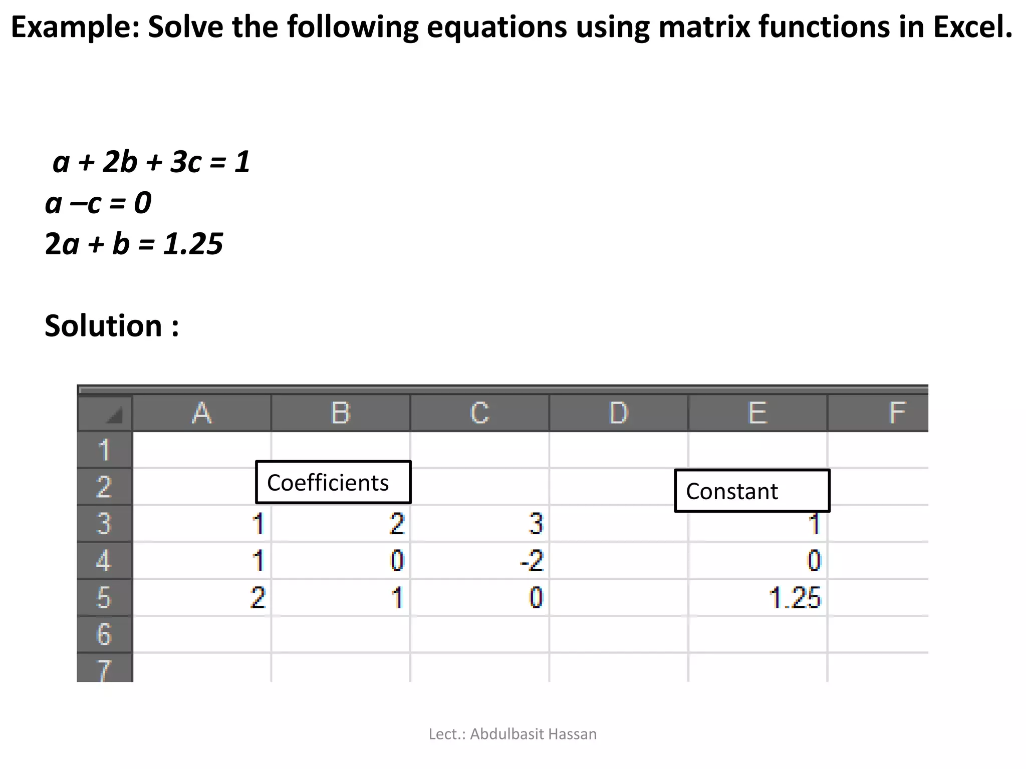
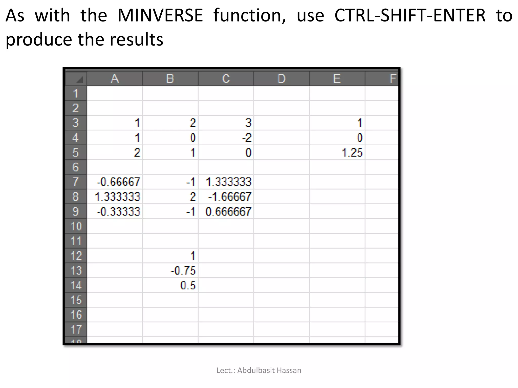
a + 2b+ 3c = 1
a –c = 0
2a + b = 1.25
Solution :
Example: Solve the following equations using matrix functions in Excel.
Coefficients Constant
Lect.: Abdulbasit Hassan
172.
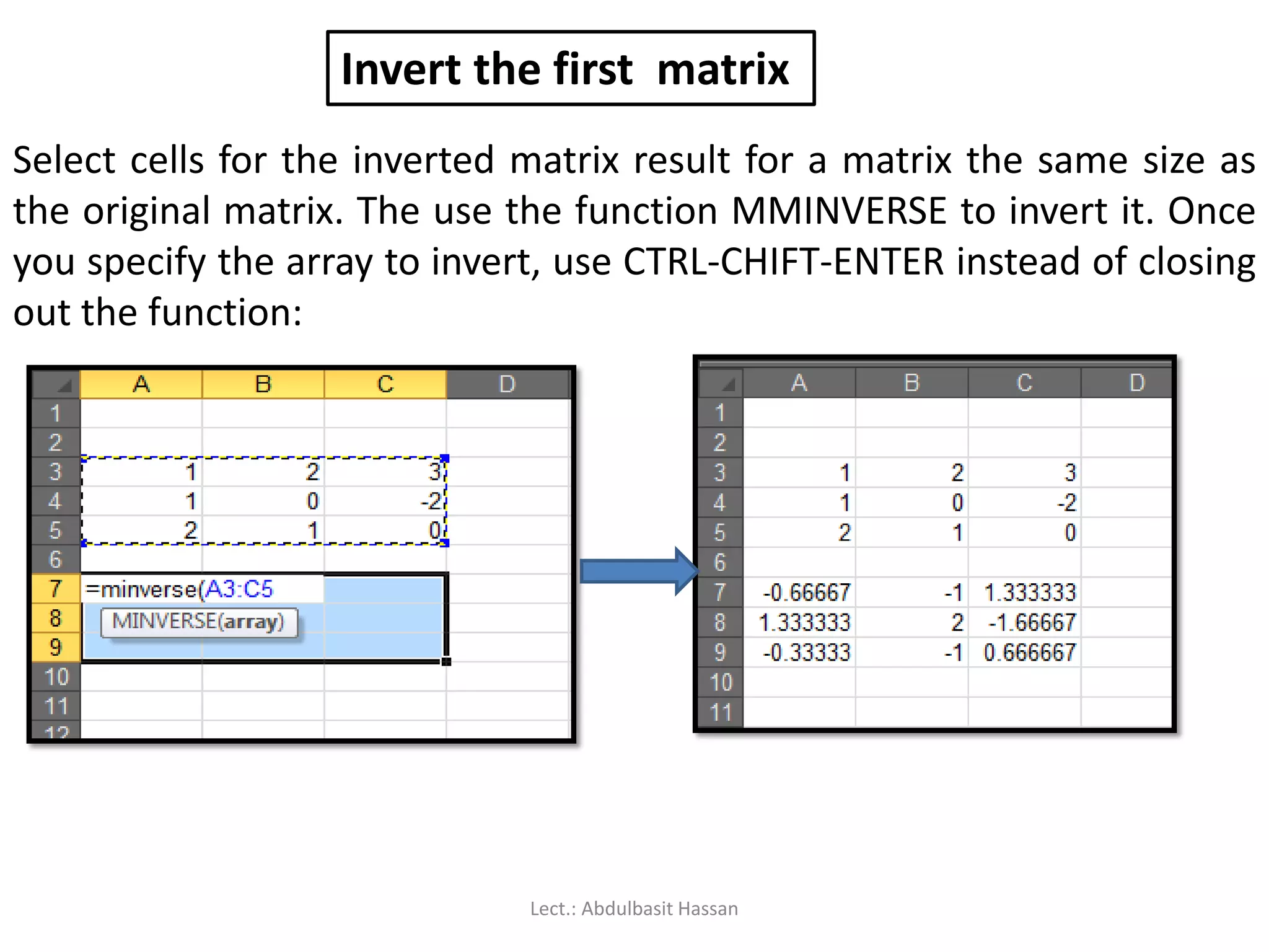
Invert the firstmatrix
Select cells for the inverted matrix result for a matrix the same size as
the original matrix. The use the function MMINVERSE to invert it. Once
you specify the array to invert, use CTRL-CHIFT-ENTER instead of closing
out the function:
Lect.: Abdulbasit Hassan
173.
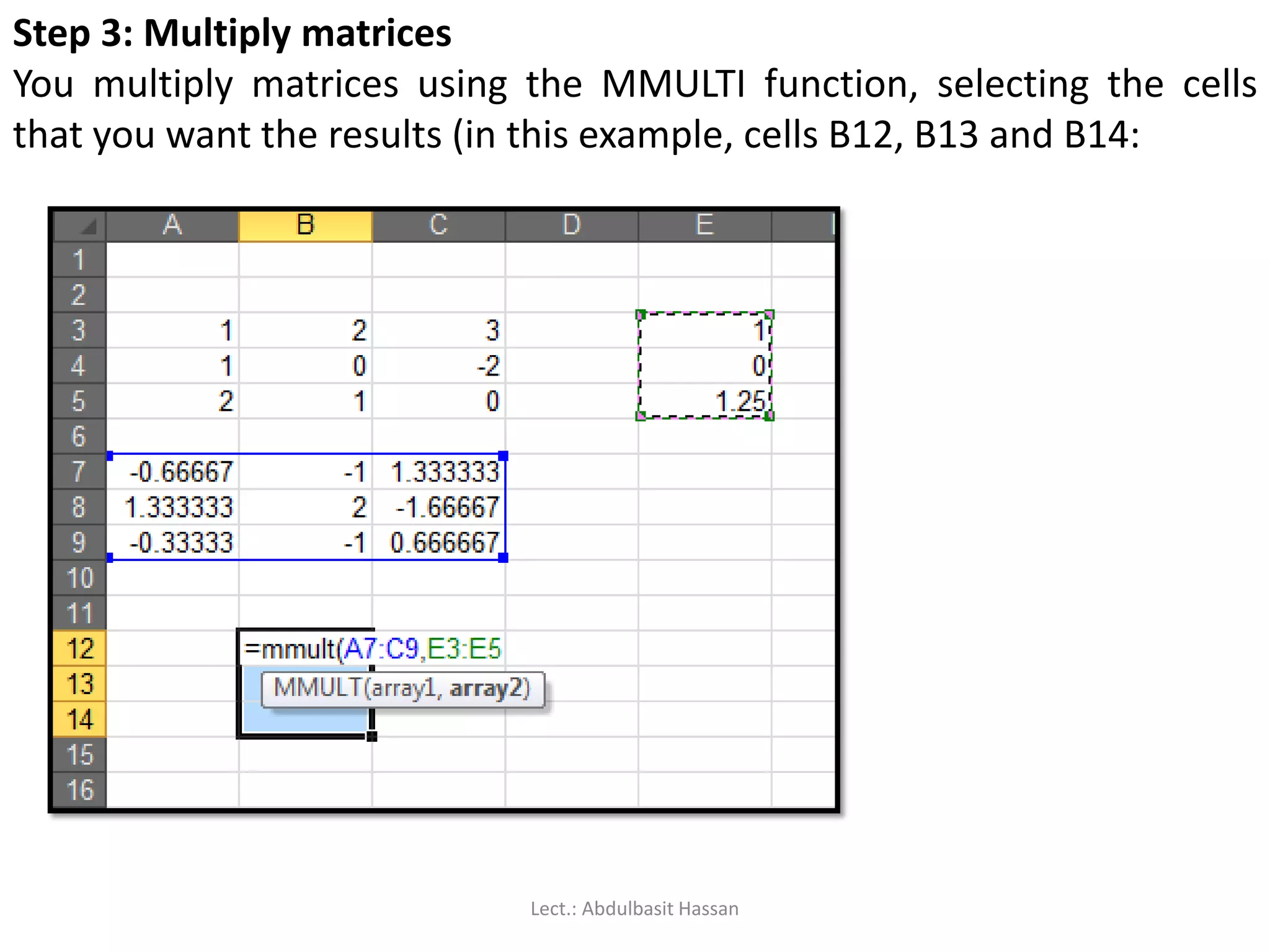
Step 3: Multiplymatrices
You multiply matrices using the MMULTI function, selecting the cells
that you want the results (in this example, cells B12, B13 and B14:
Lect.: Abdulbasit Hassan
174.
As with theMINVERSE function, use CTRL-SHIFT-ENTER to
produce the results
Lect.: Abdulbasit Hassan
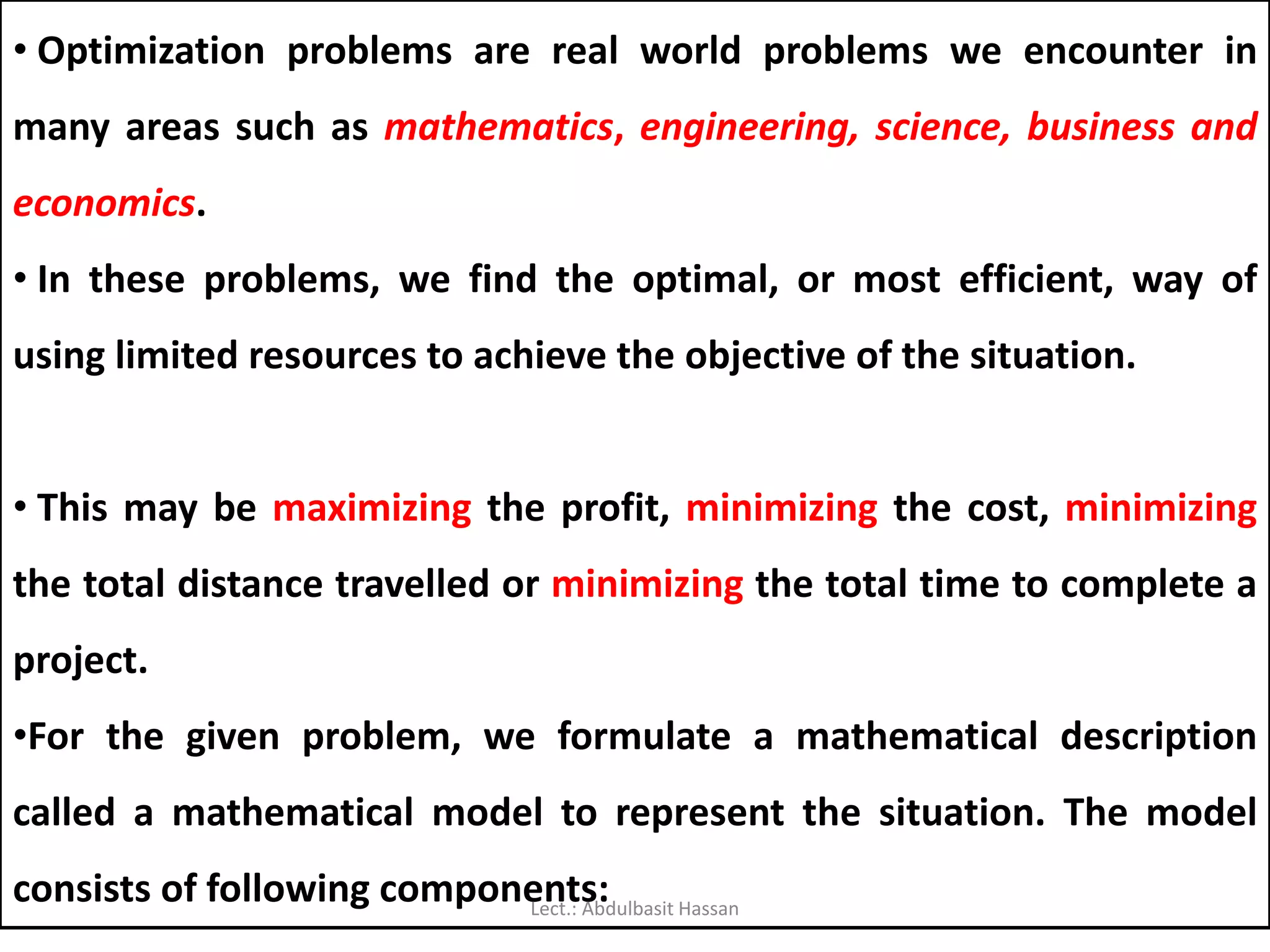
• Optimization problemsare real world problems we encounter in
many areas such as mathematics, engineering, science, business and
economics.
• In these problems, we find the optimal, or most efficient, way of
using limited resources to achieve the objective of the situation.
• This may be maximizing the profit, minimizing the cost, minimizing
the total distance travelled or minimizing the total time to complete a
project.
•For the given problem, we formulate a mathematical description
called a mathematical model to represent the situation. The model
consists of following components:Lect.: Abdulbasit Hassan
178.
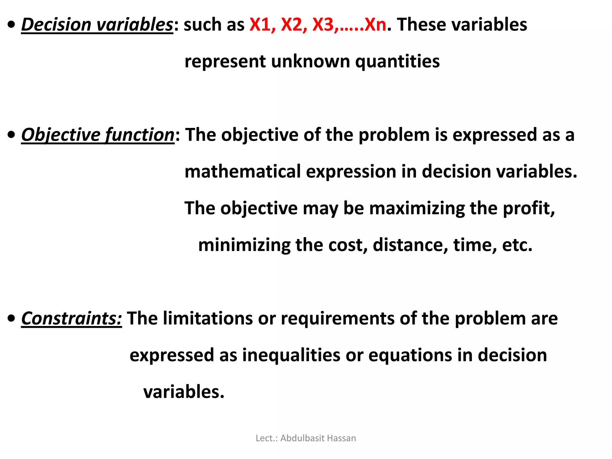
• Decision variables:such as X1, X2, X3,…..Xn. These variables
represent unknown quantities
• Objective function: The objective of the problem is expressed as a
mathematical expression in decision variables.
The objective may be maximizing the profit,
minimizing the cost, distance, time, etc.
• Constraints: The limitations or requirements of the problem are
expressed as inequalities or equations in decision
variables.
Lect.: Abdulbasit Hassan
179.
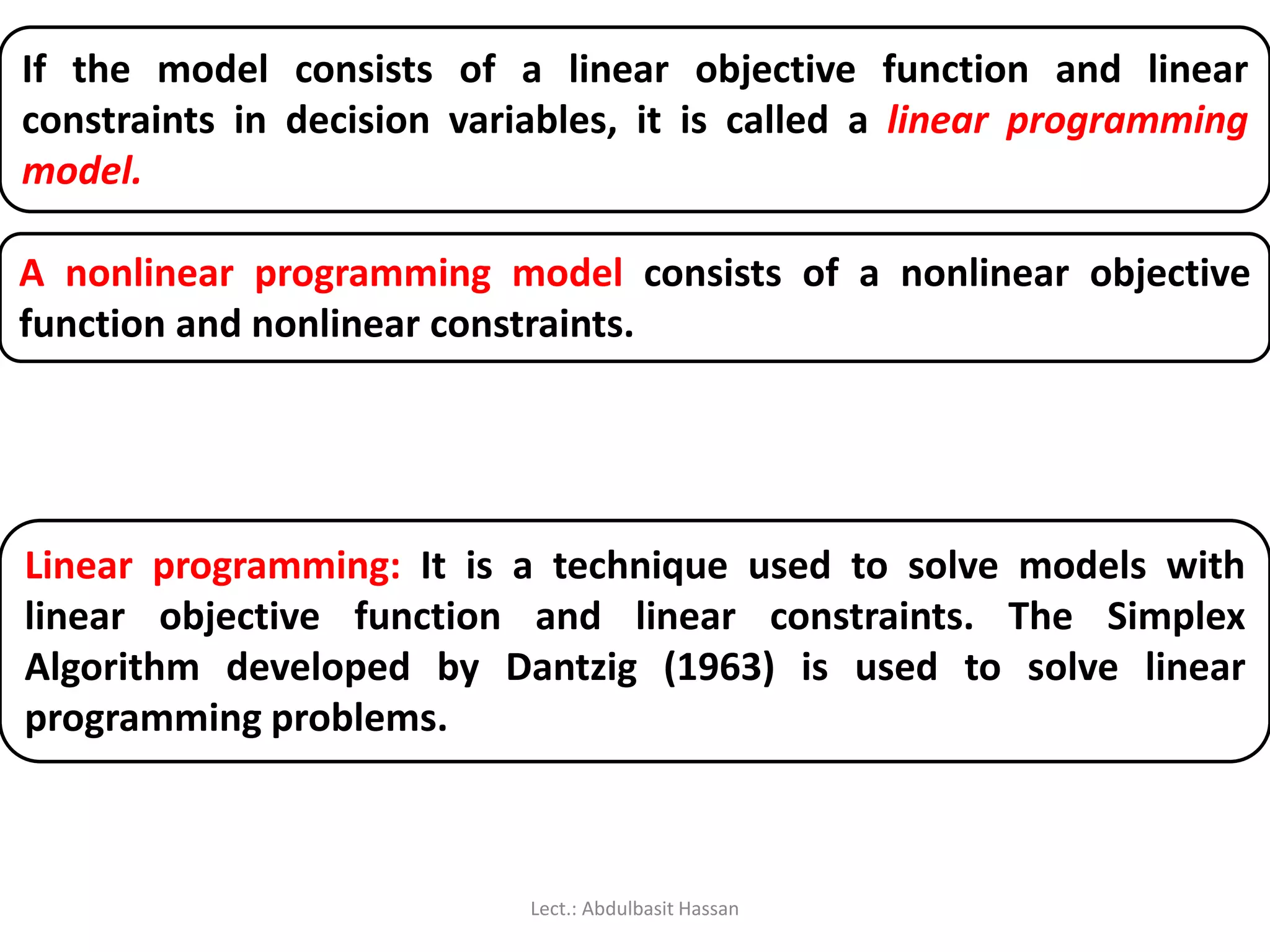
If the modelconsists of a linear objective function and linear
constraints in decision variables, it is called a linear programming
model.
A nonlinear programming model consists of a nonlinear objective
function and nonlinear constraints.
Linear programming: It is a technique used to solve models with
linear objective function and linear constraints. The Simplex
Algorithm developed by Dantzig (1963) is used to solve linear
programming problems.
Lect.: Abdulbasit Hassan
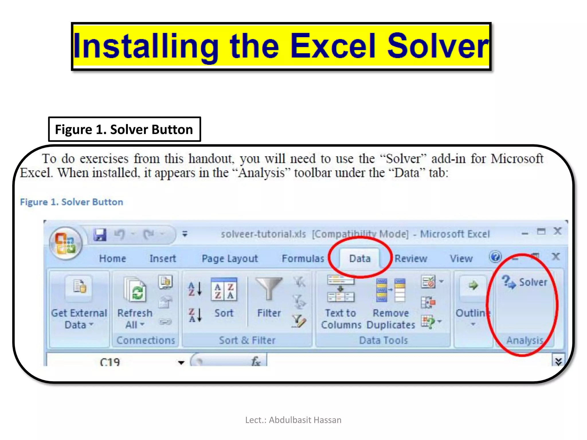
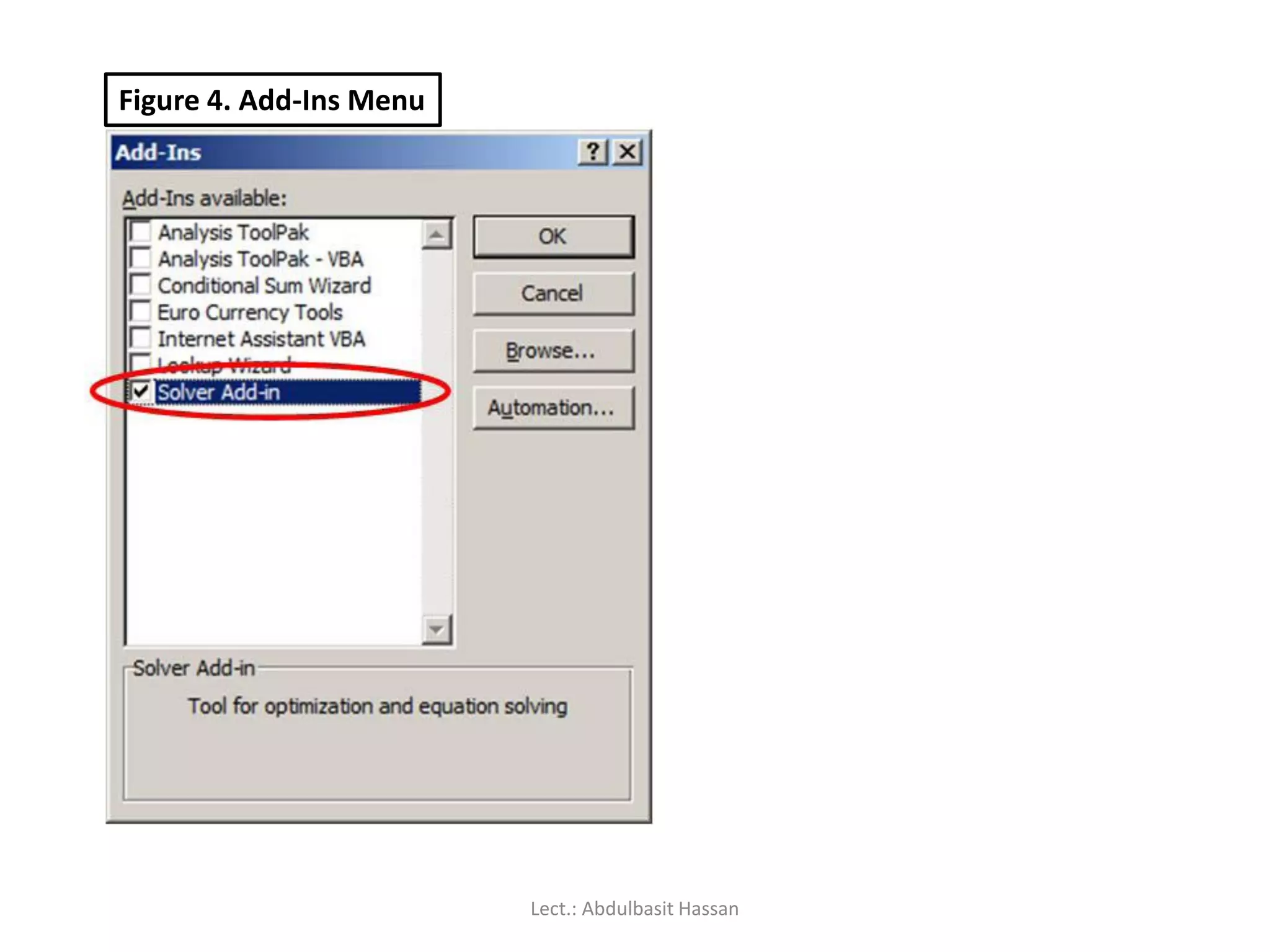
If the “Analysis”toolbar does not appear, or does not have the
“Solver” button, the add-in must first be activated:
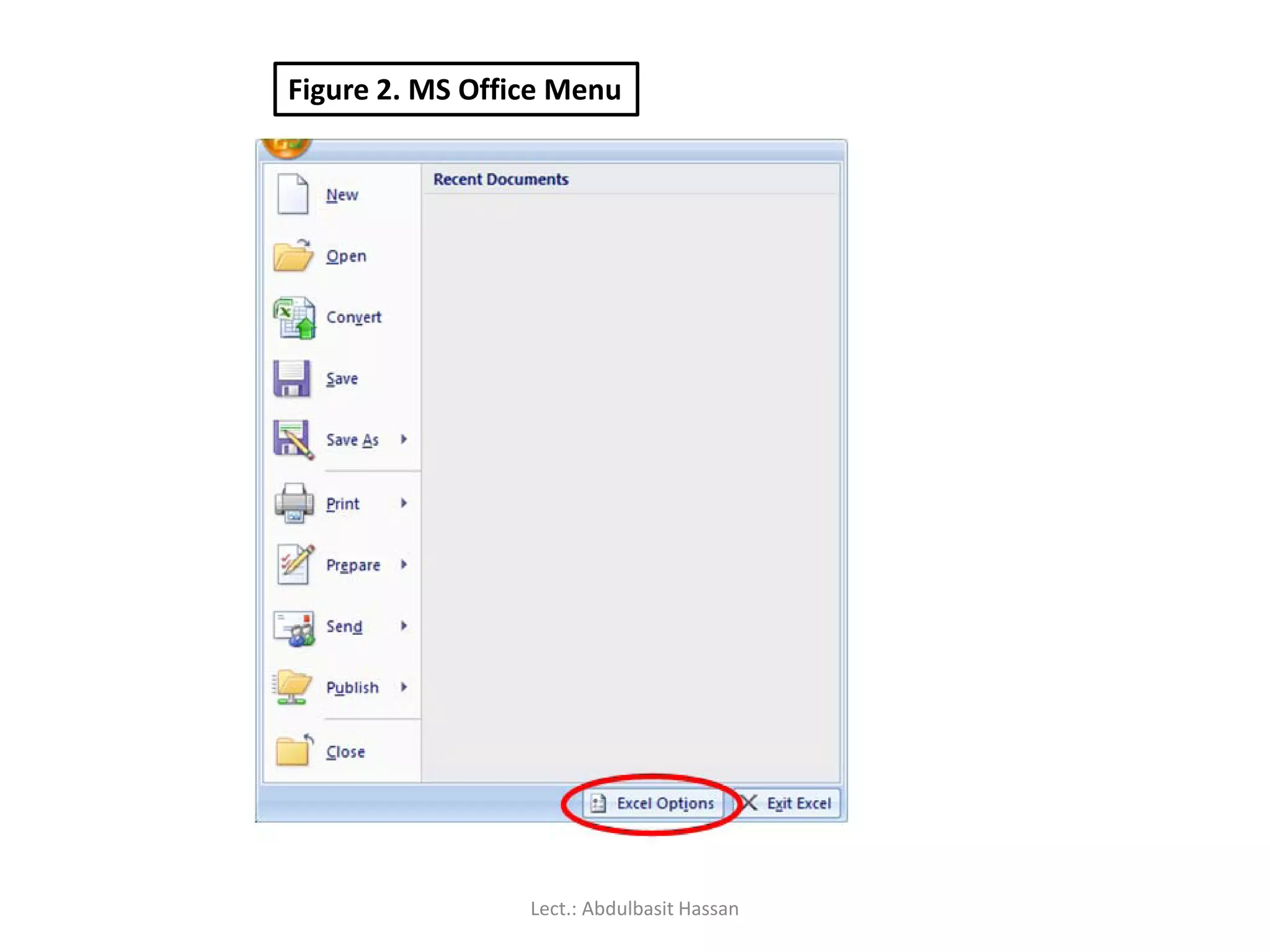
1. Click on the “Office” button in the top left corner:
2. Choose “Excel Options” (Figure 2)
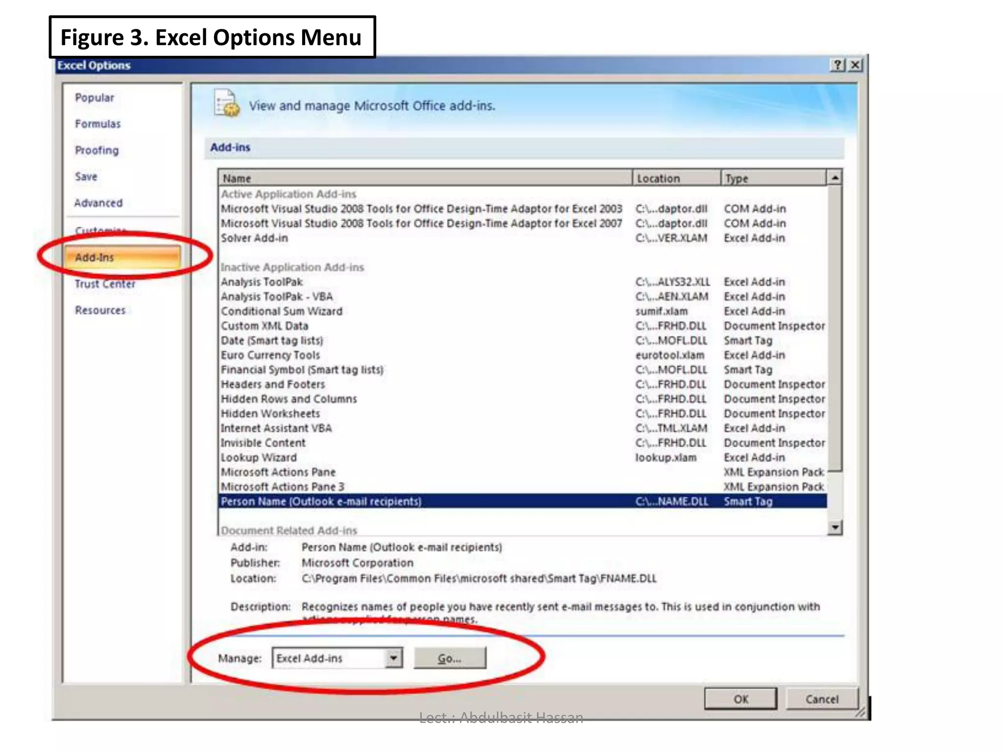
3. Choose “Add-Ins” in the vertical menu on the left (Figure 3)
4. Pick “Excel Add-Ins” from the “Manage” box and click “Go…”(Figure 3)
5. Check “Solver Add-In” and press “OK” (Figure 4)
6. The Solver add-in should now appear in the Analysis toolbar (Figure 1)
Lect.: Abdulbasit Hassan
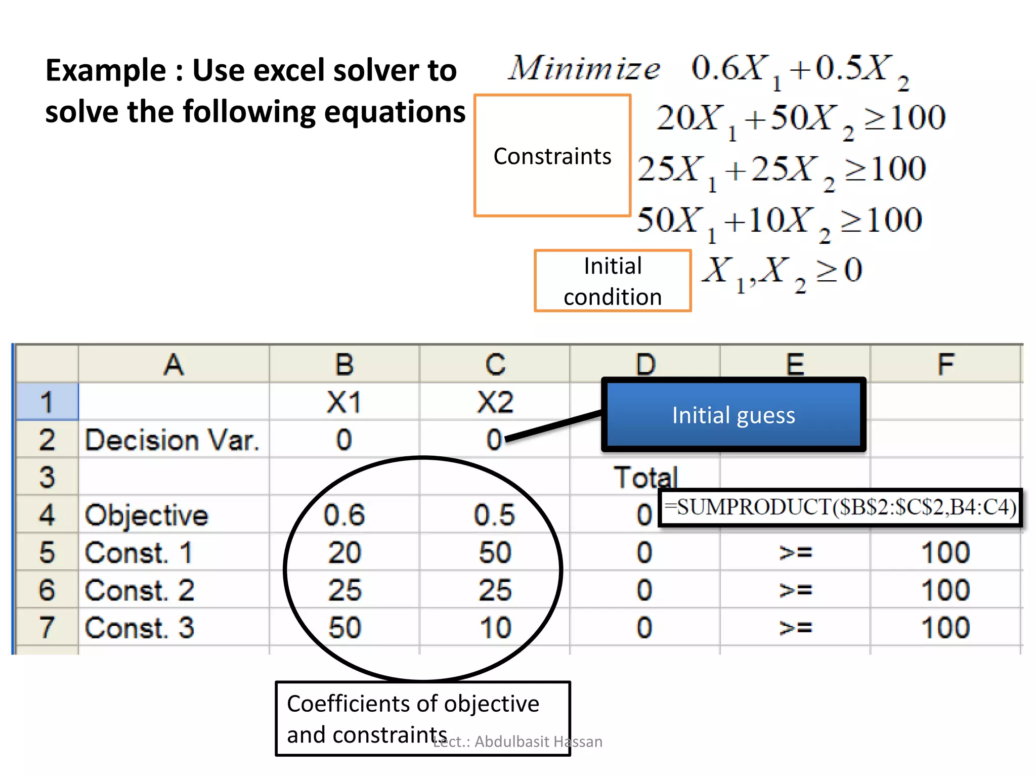
Example : Useexcel solver to
solve the following equations
Initial guess
Coefficients of objective
and constraints
Constraints
Initial
condition
Lect.: Abdulbasit Hassan
186.
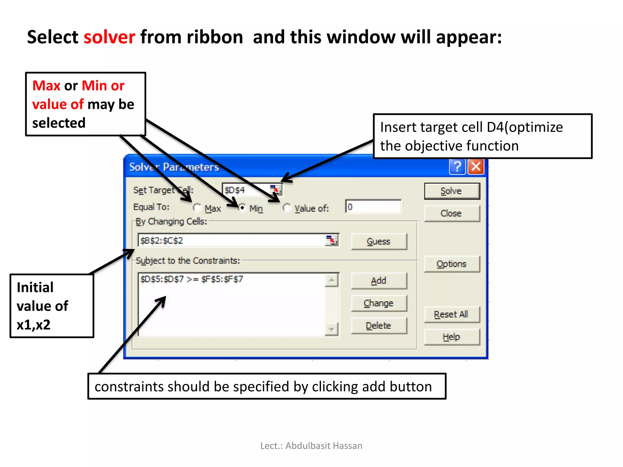
Select solver fromribbon and this window will appear:
Insert target cell D4(optimize
the objective function
Max or Min or
value of may be
selected
Initial
value of
x1,x2
constraints should be specified by clicking add button
Lect.: Abdulbasit Hassan
187.
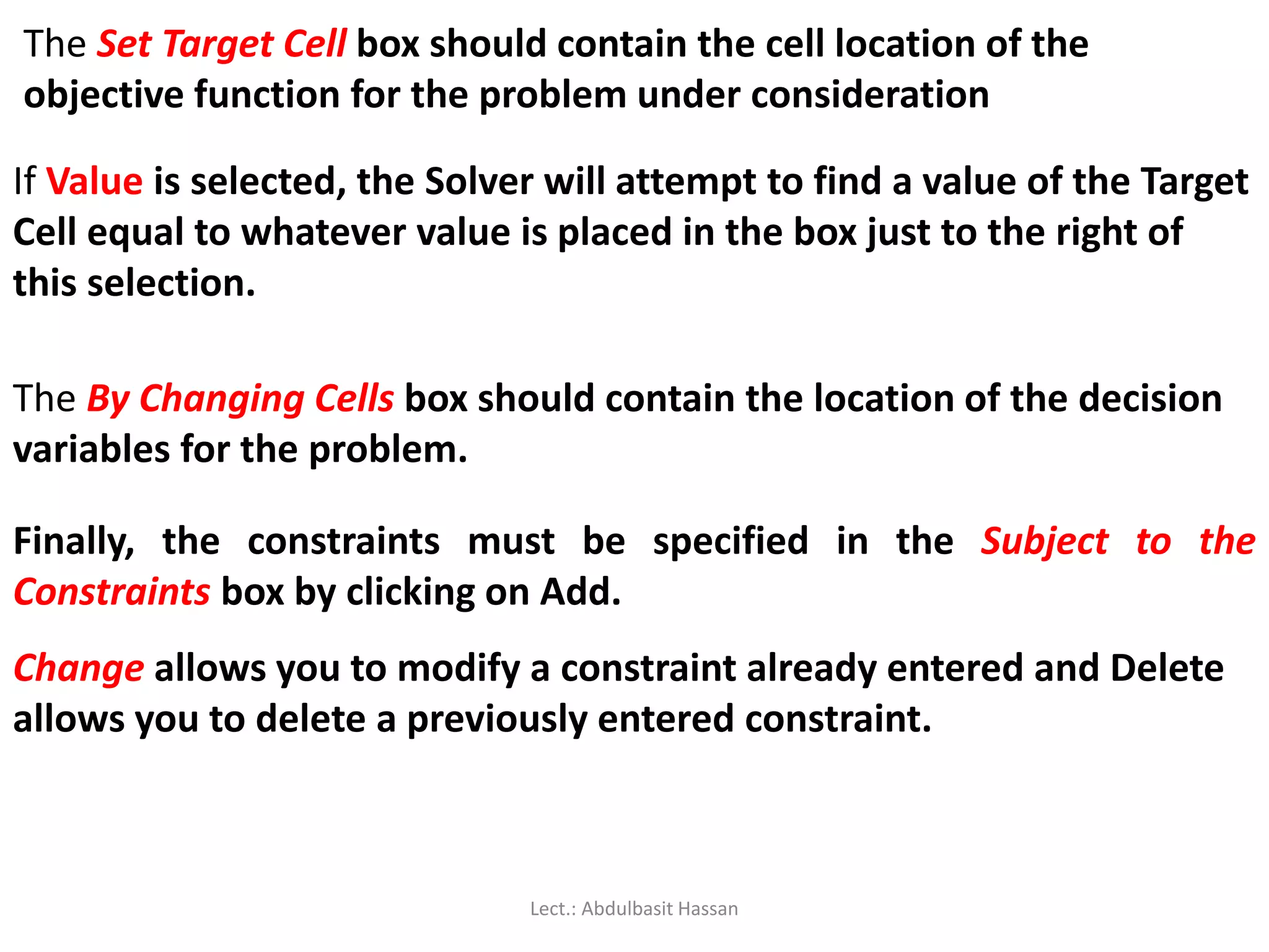
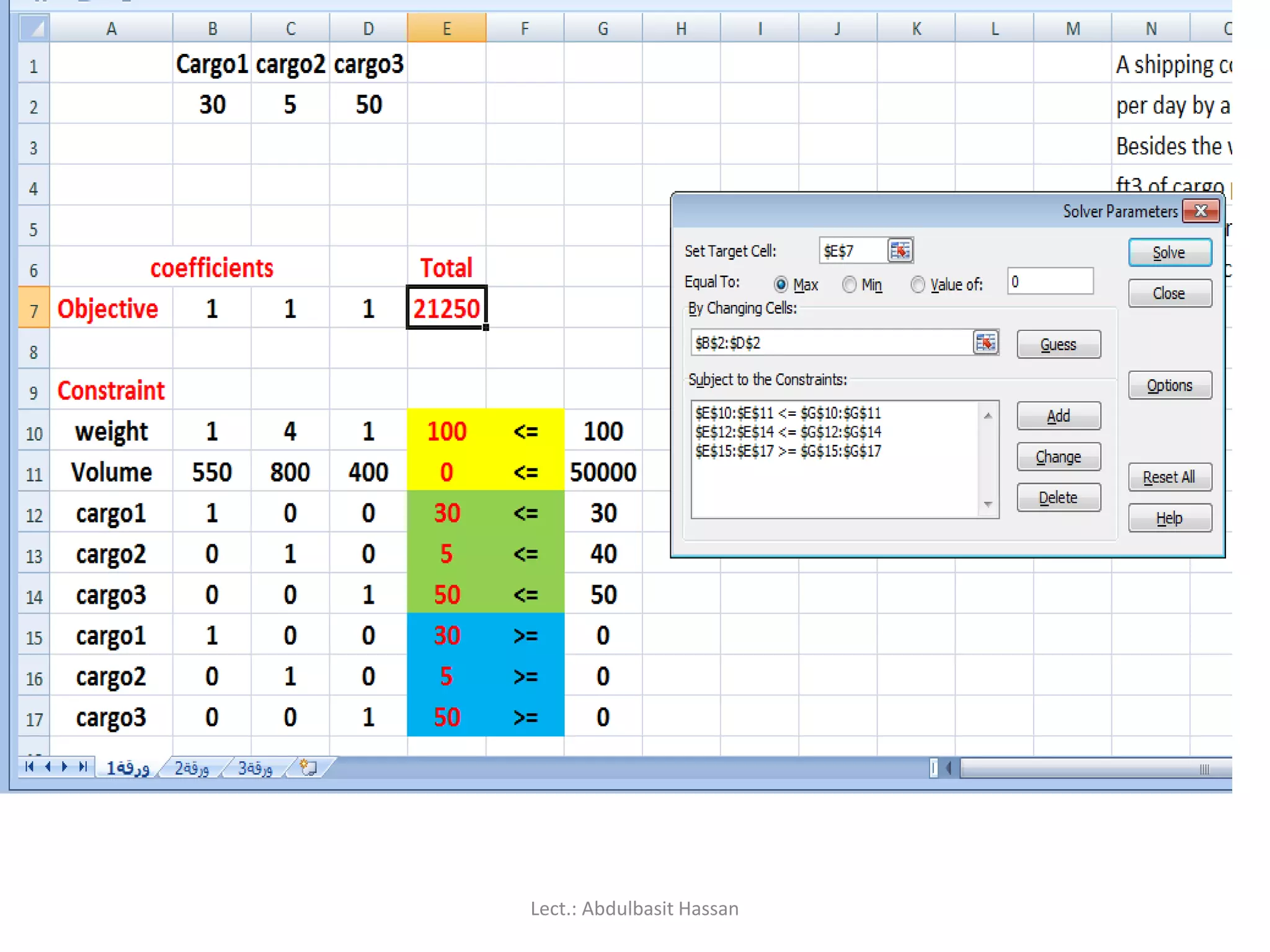
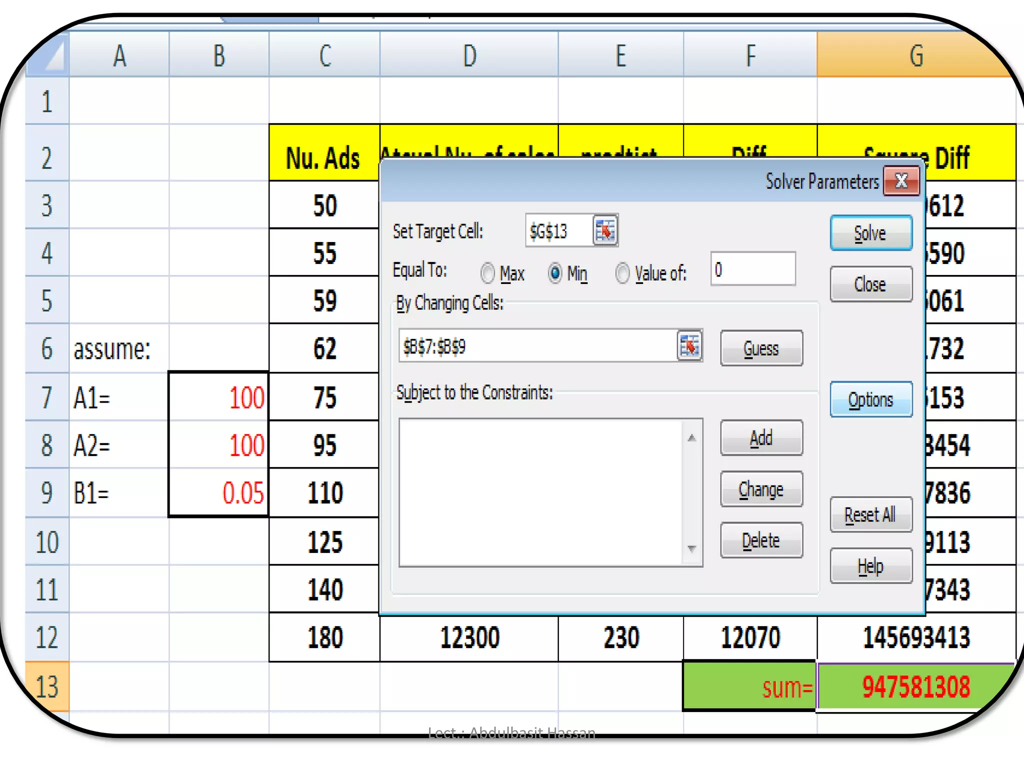
The Set TargetCell box should contain the cell location of the
objective function for the problem under consideration
If Value is selected, the Solver will attempt to find a value of the Target
Cell equal to whatever value is placed in the box just to the right of
this selection.
The By Changing Cells box should contain the location of the decision
variables for the problem.
Finally, the constraints must be specified in the Subject to the
Constraints box by clicking on Add.
Change allows you to modify a constraint already entered and Delete
allows you to delete a previously entered constraint.
Lect.: Abdulbasit Hassan
188.
Reset All clearsthe current problem and resets all parameters to their
default values.
Options invokes the Solver options dialog box (to be discussed later).
The Guess selection is not particularly useful for our purposes and will
not be discussed here.
When the Add button is clicked, the Add Constraint dialog box
appears:
Lect.: Abdulbasit Hassan
189.
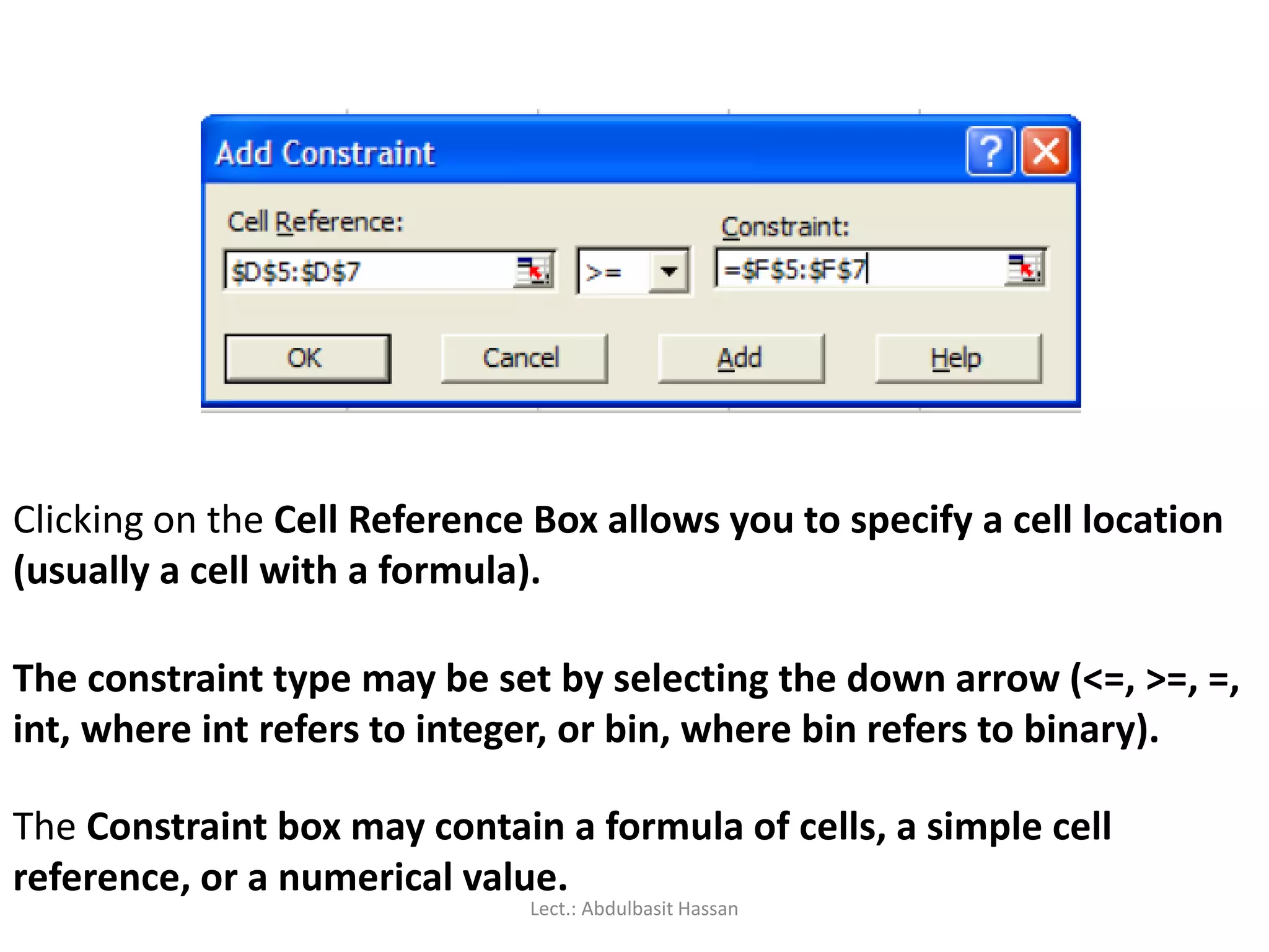
Clicking on theCell Reference Box allows you to specify a cell location
(usually a cell with a formula).
The constraint type may be set by selecting the down arrow (<=, >=, =,
int, where int refers to integer, or bin, where bin refers to binary).
The Constraint box may contain a formula of cells, a simple cell
reference, or a numerical value.
Lect.: Abdulbasit Hassan
190.
The Add buttonadds the currently specified constraint to the existing
model and returns to the Add Constraint dialog box
The OK button adds the current constraint to the model and returns
you to the Solver Dialog box.
Lect.: Abdulbasit Hassan
191.
Note: Solver doesnot assume nonnegative of the decision variables.
The options dialog box discussed below allows you to specify that the
variables must be nonnegative.
Max Time allows you to set the number of seconds before Solver will
stop. Iterations, similar to Max Time,
Precision is the degree of accuracy of the solver algorithm
If you seek the optimal solution, Tolerance must be set to zero
If run time becomes too long, you may wish to set this to a higher
value (if you are willing to accept a solution within this percent of
optimality).
Lect.: Abdulbasit Hassan
192.
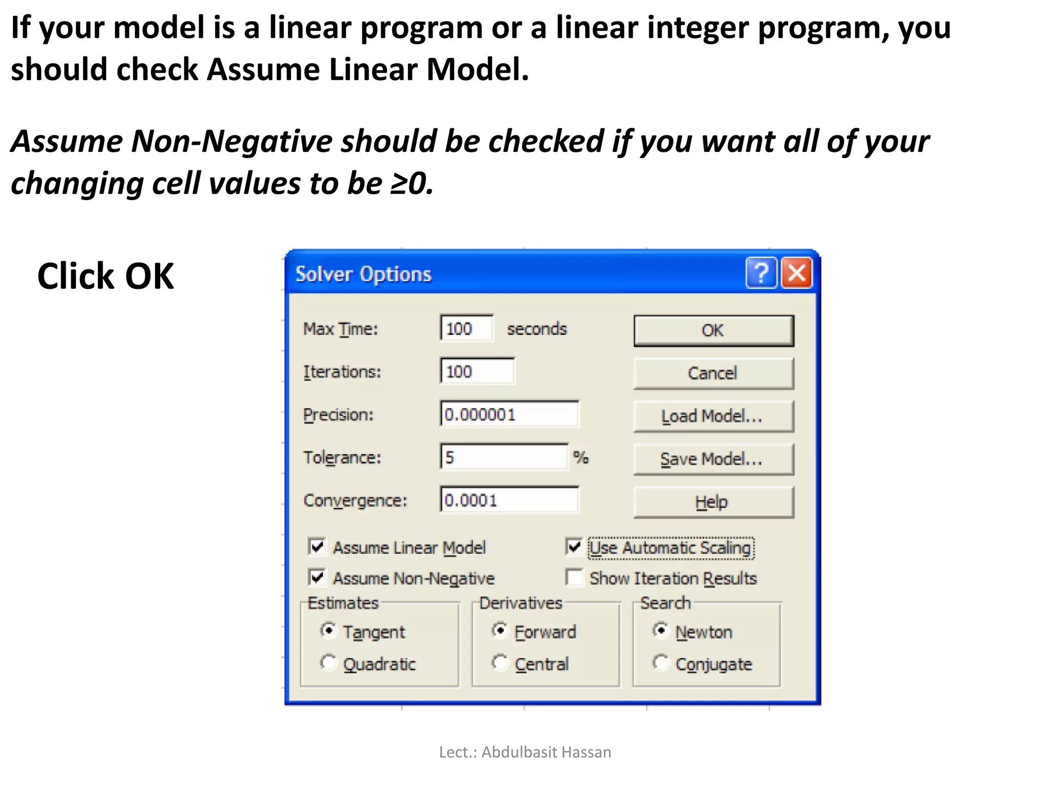
If your modelis a linear program or a linear integer program, you
should check Assume Linear Model.
Assume Non-Negative should be checked if you want all of your
changing cell values to be ≥0.
Click OK
Lect.: Abdulbasit Hassan
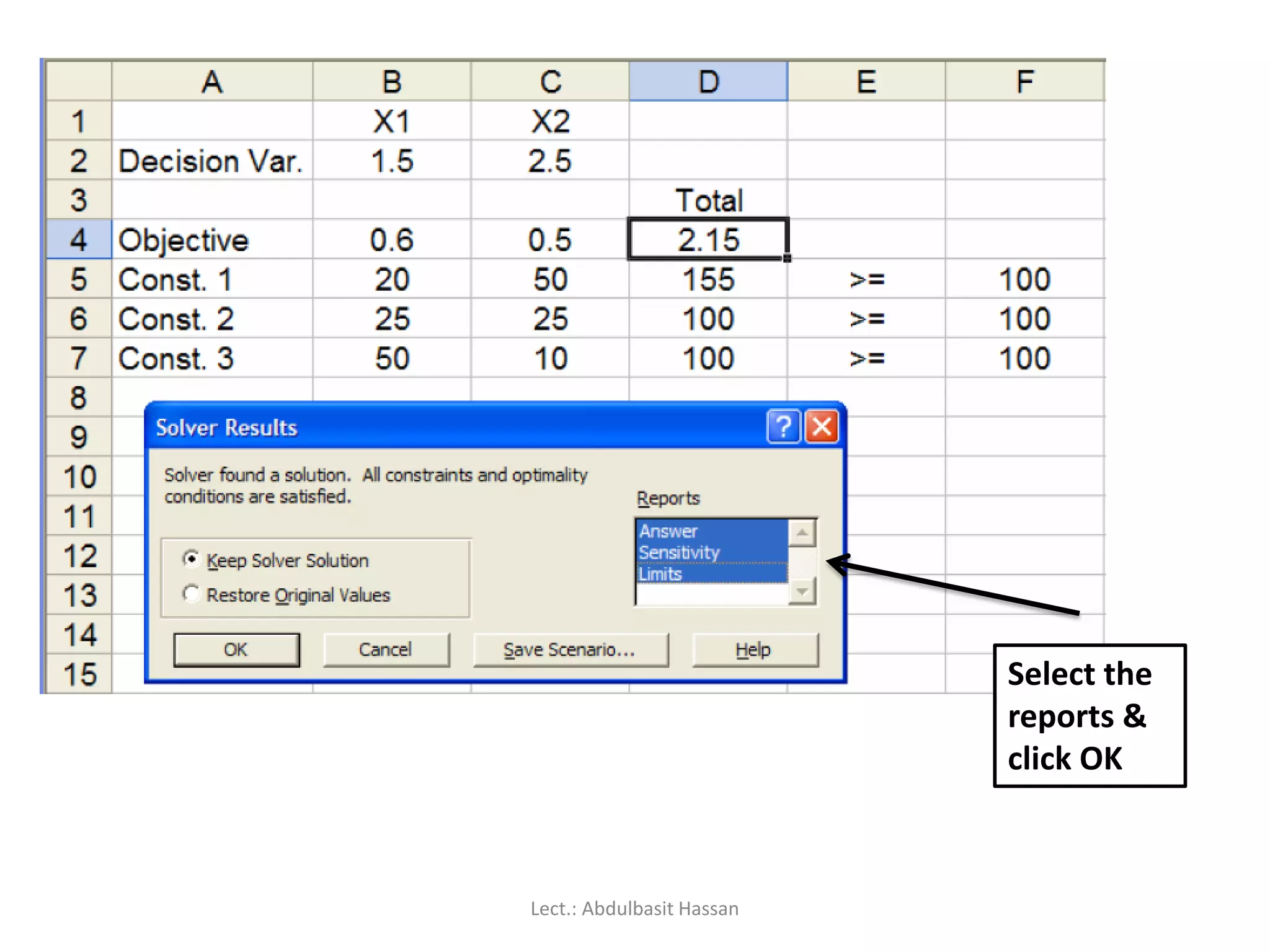
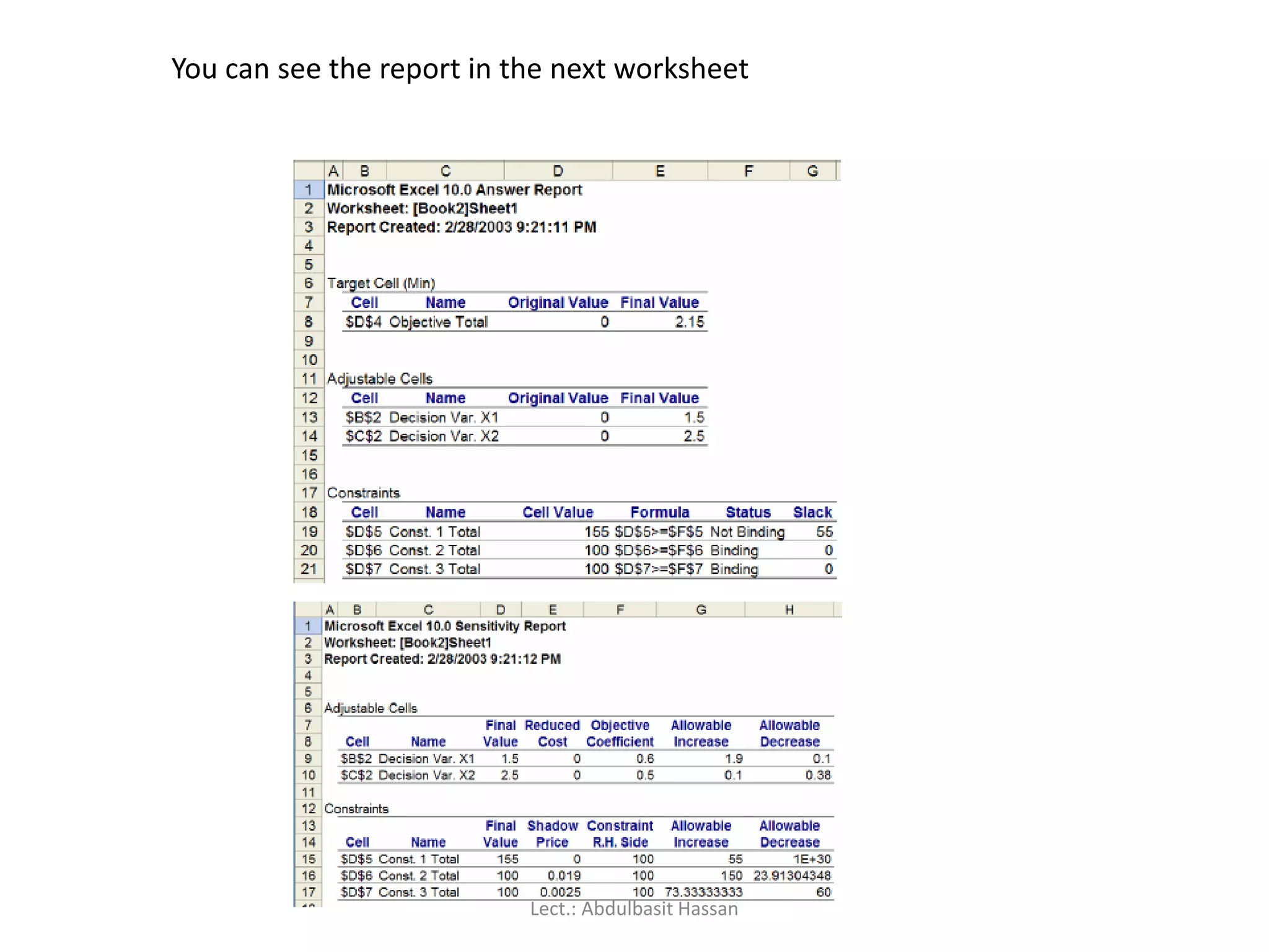
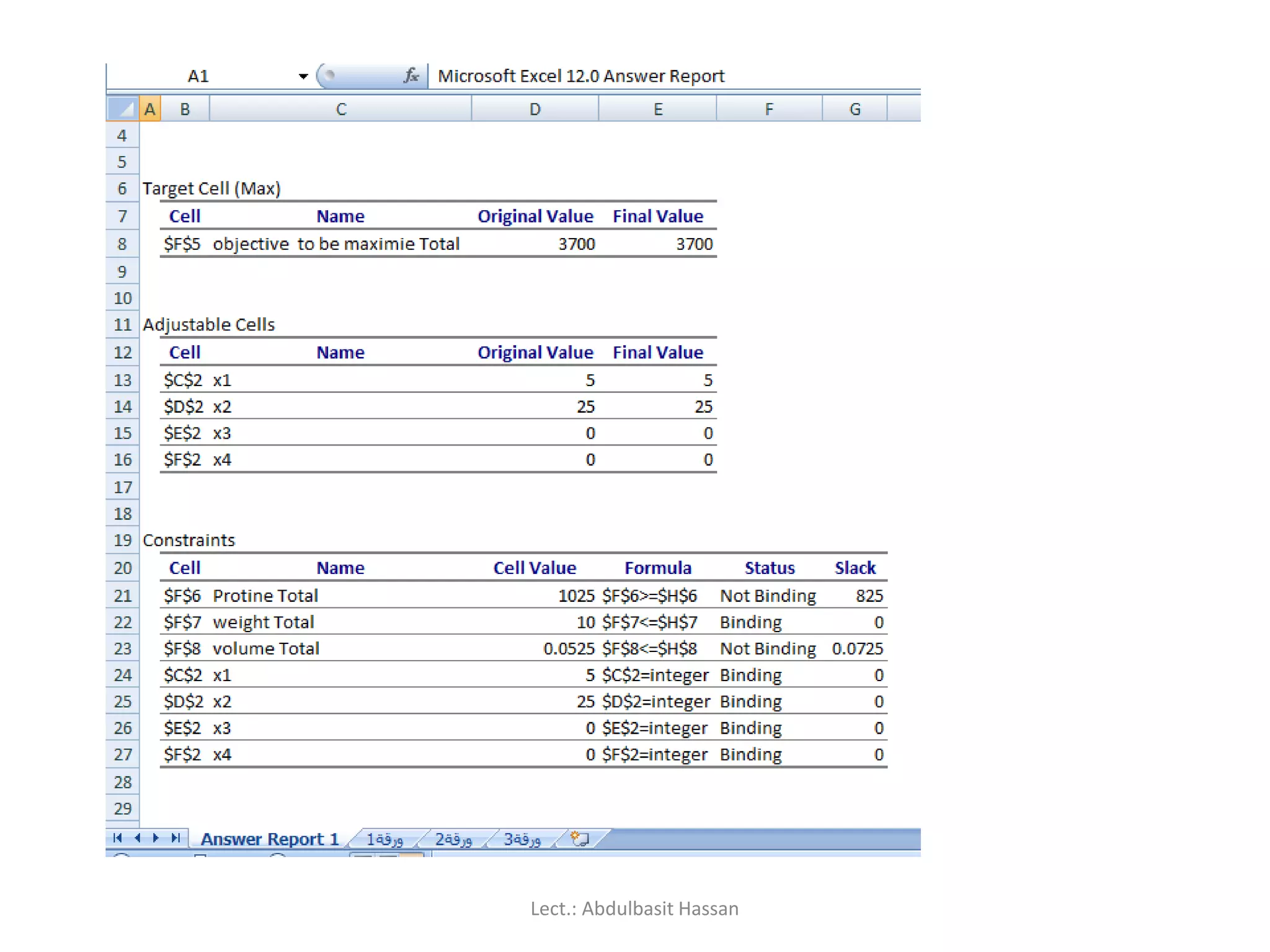
You can seethe report in the next worksheet
Lect.: Abdulbasit Hassan
195.
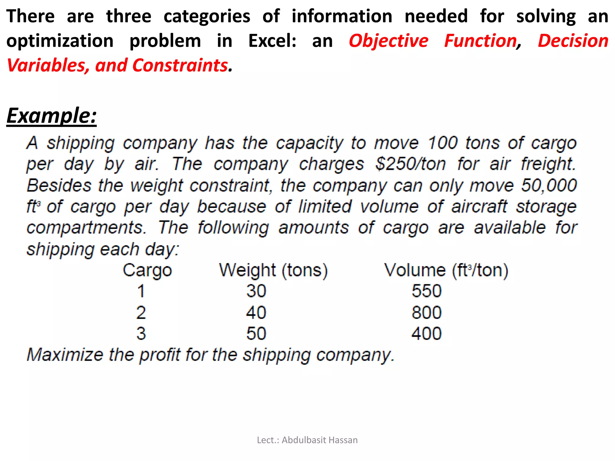
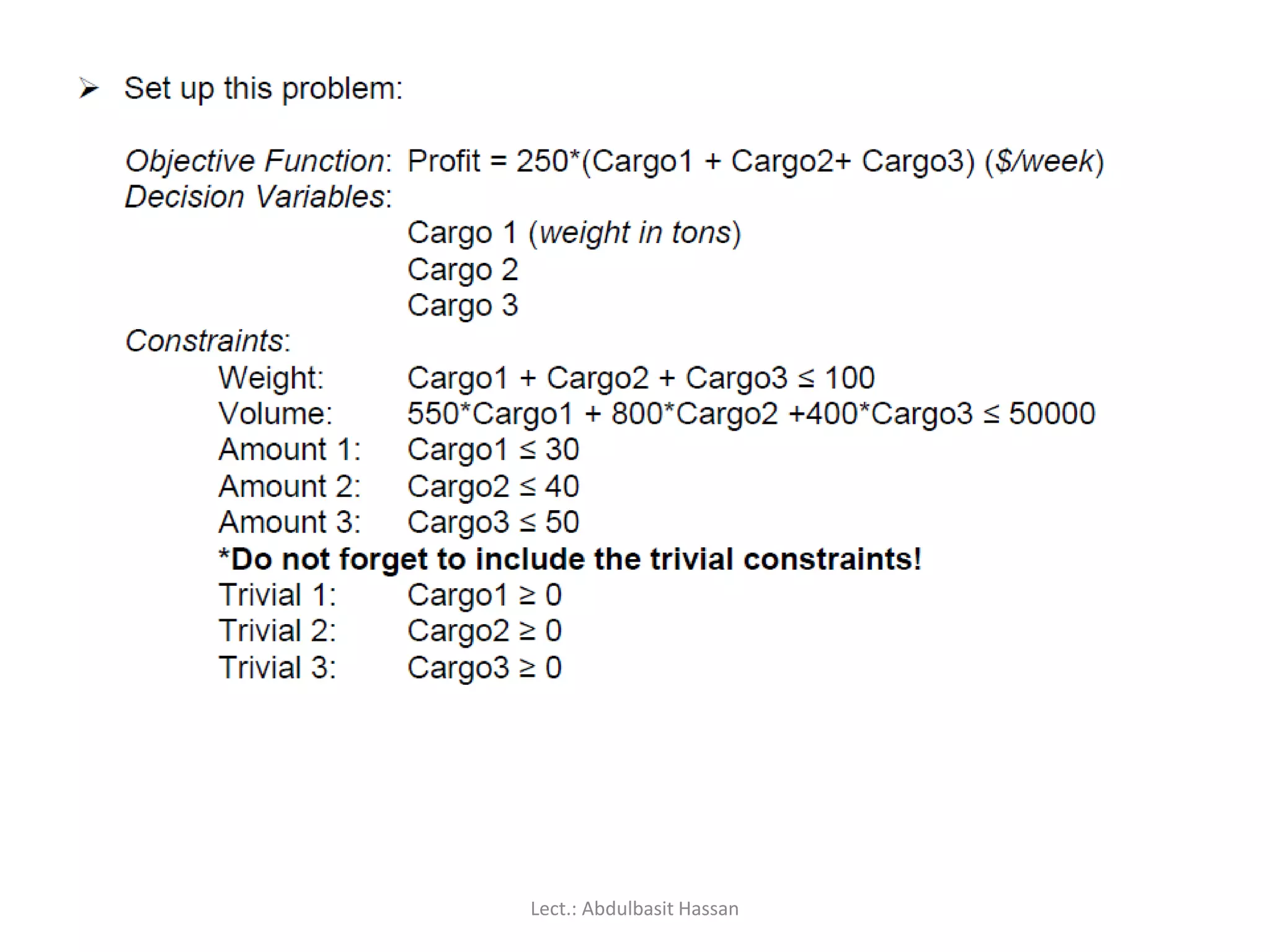
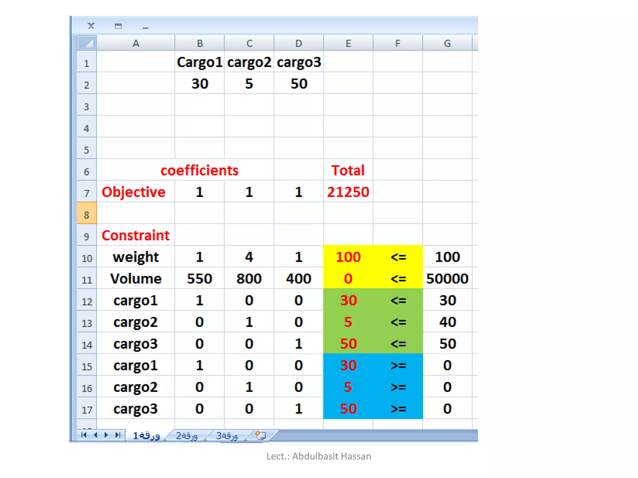
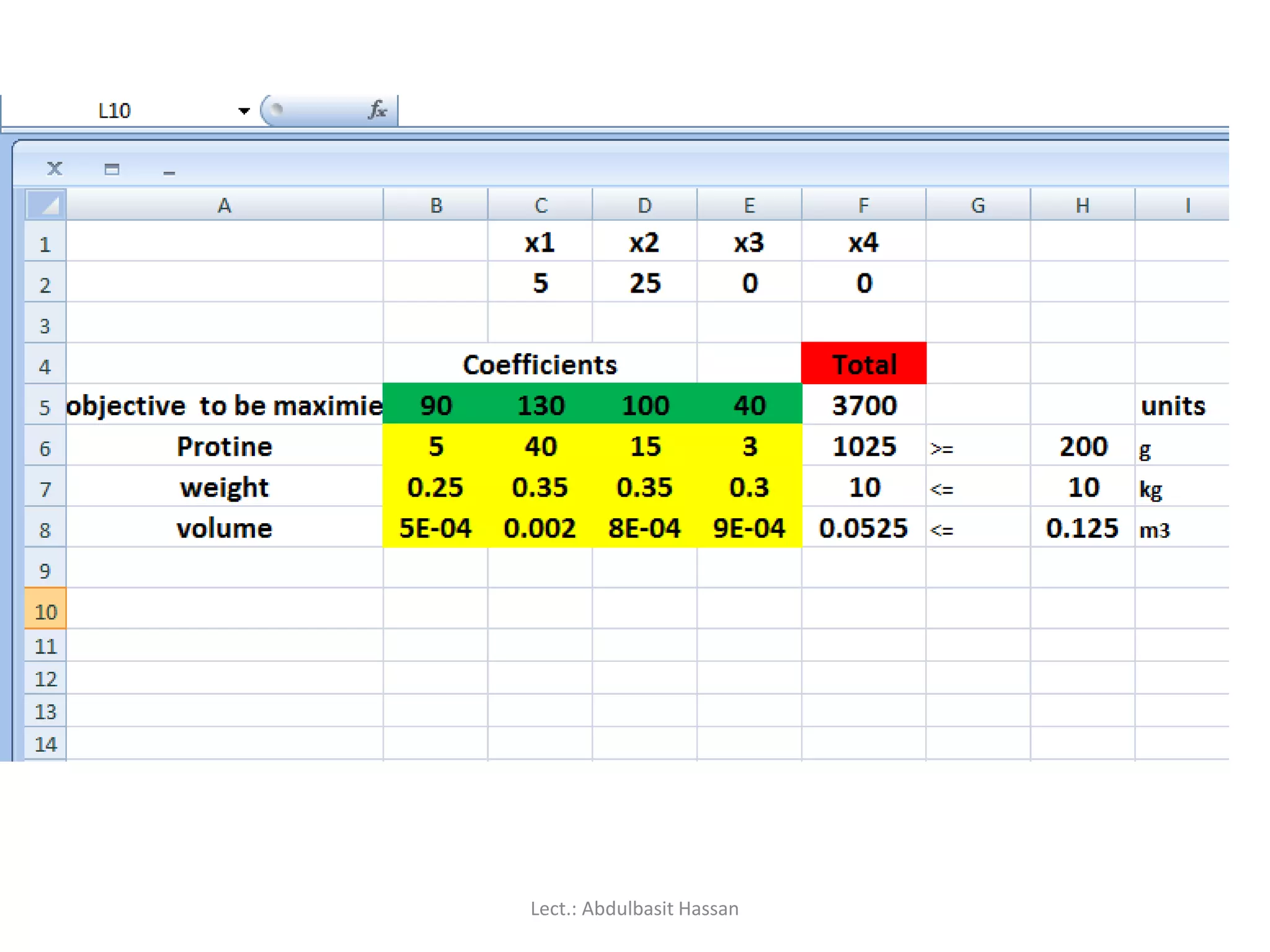
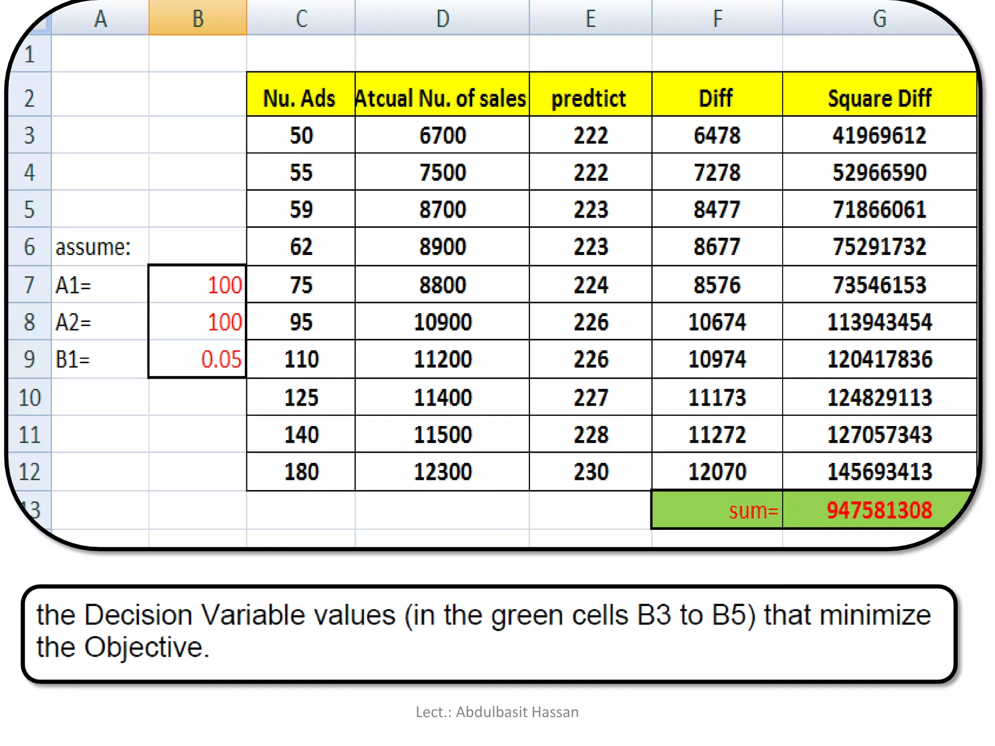
There are threecategories of information needed for solving an
optimization problem in Excel: an Objective Function, Decision
Variables, and Constraints.
Example:
Lect.: Abdulbasit Hassan
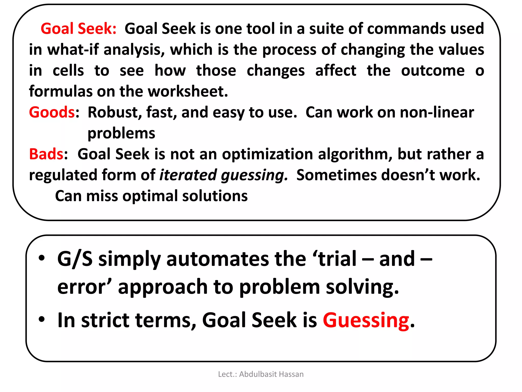
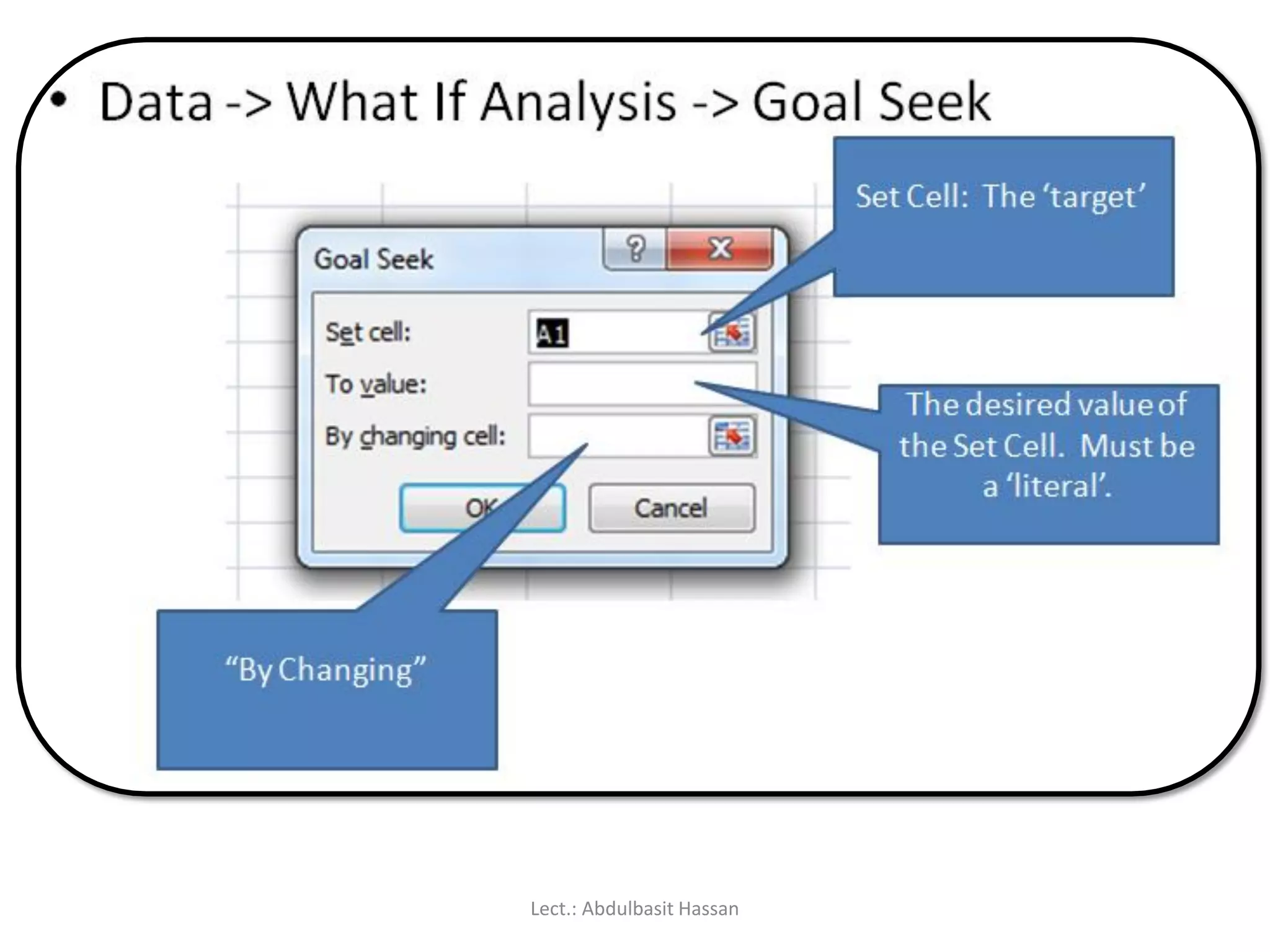
Goal Seek: GoalSeek is one tool in a suite of commands used
in what-if analysis, which is the process of changing the values
in cells to see how those changes affect the outcome o
formulas on the worksheet.
Goods: Robust, fast, and easy to use. Can work on non-linear
problems
Bads: Goal Seek is not an optimization algorithm, but rather a
regulated form of iterated guessing. Sometimes doesn’t work.
Can miss optimal solutions
• G/S simply automates the ‘trial – and –
error’ approach to problem solving.
• In strict terms, Goal Seek is Guessing.
Lect.: Abdulbasit Hassan
204.
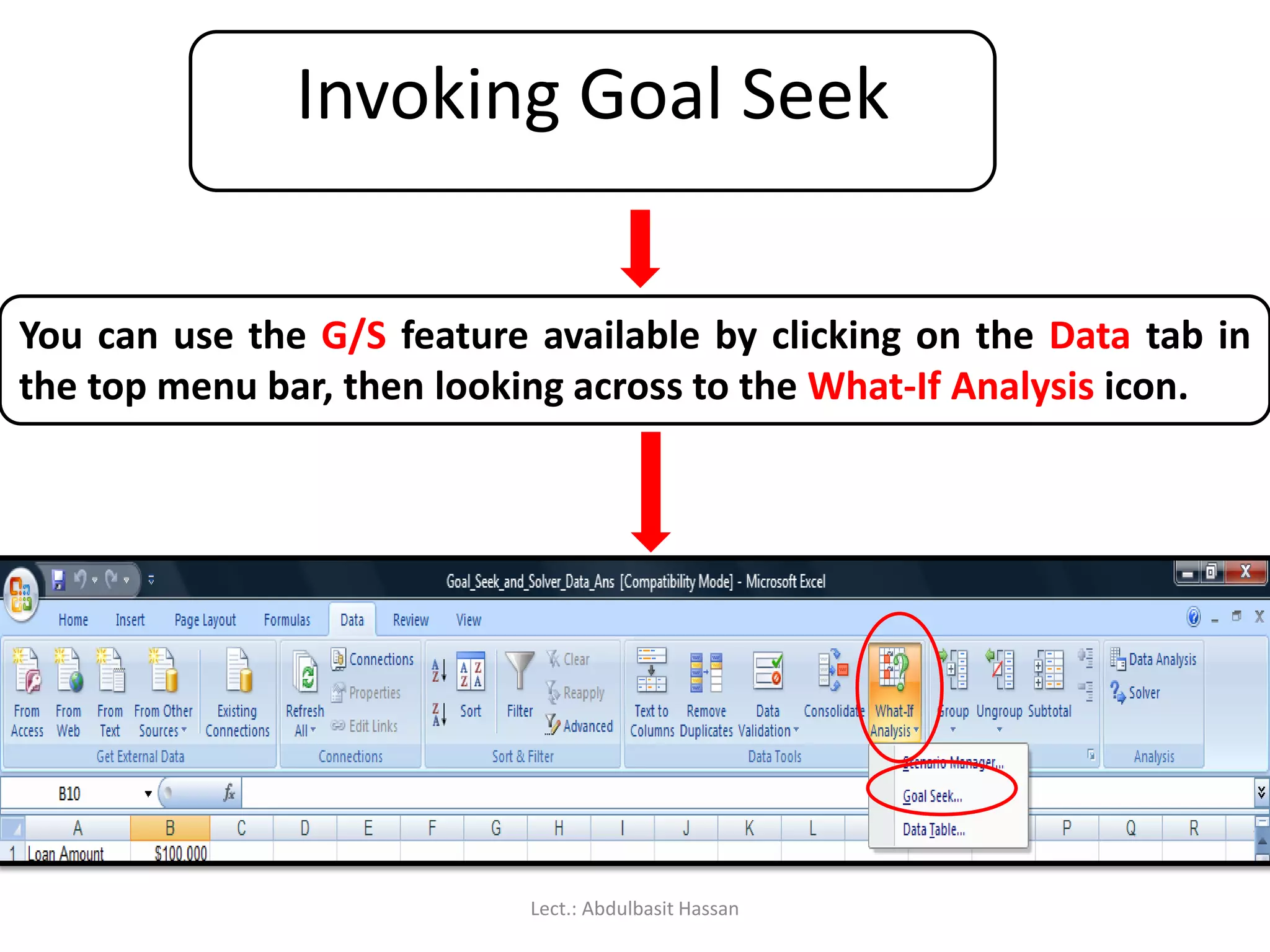
Invoking Goal Seek
Youcan use the G/S feature available by clicking on the Data tab in
the top menu bar, then looking across to the What-If Analysis icon.
Lect.: Abdulbasit Hassan
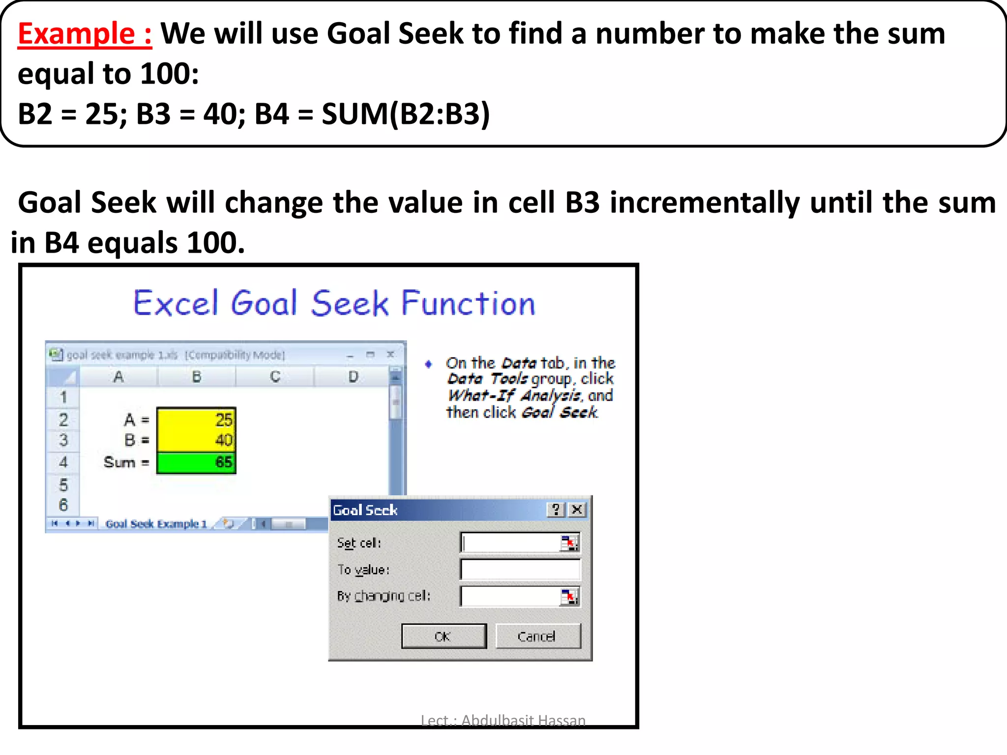
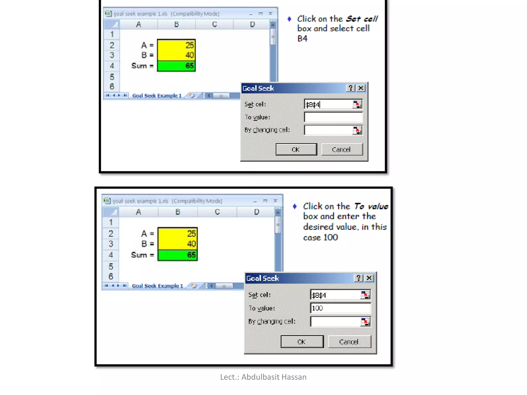
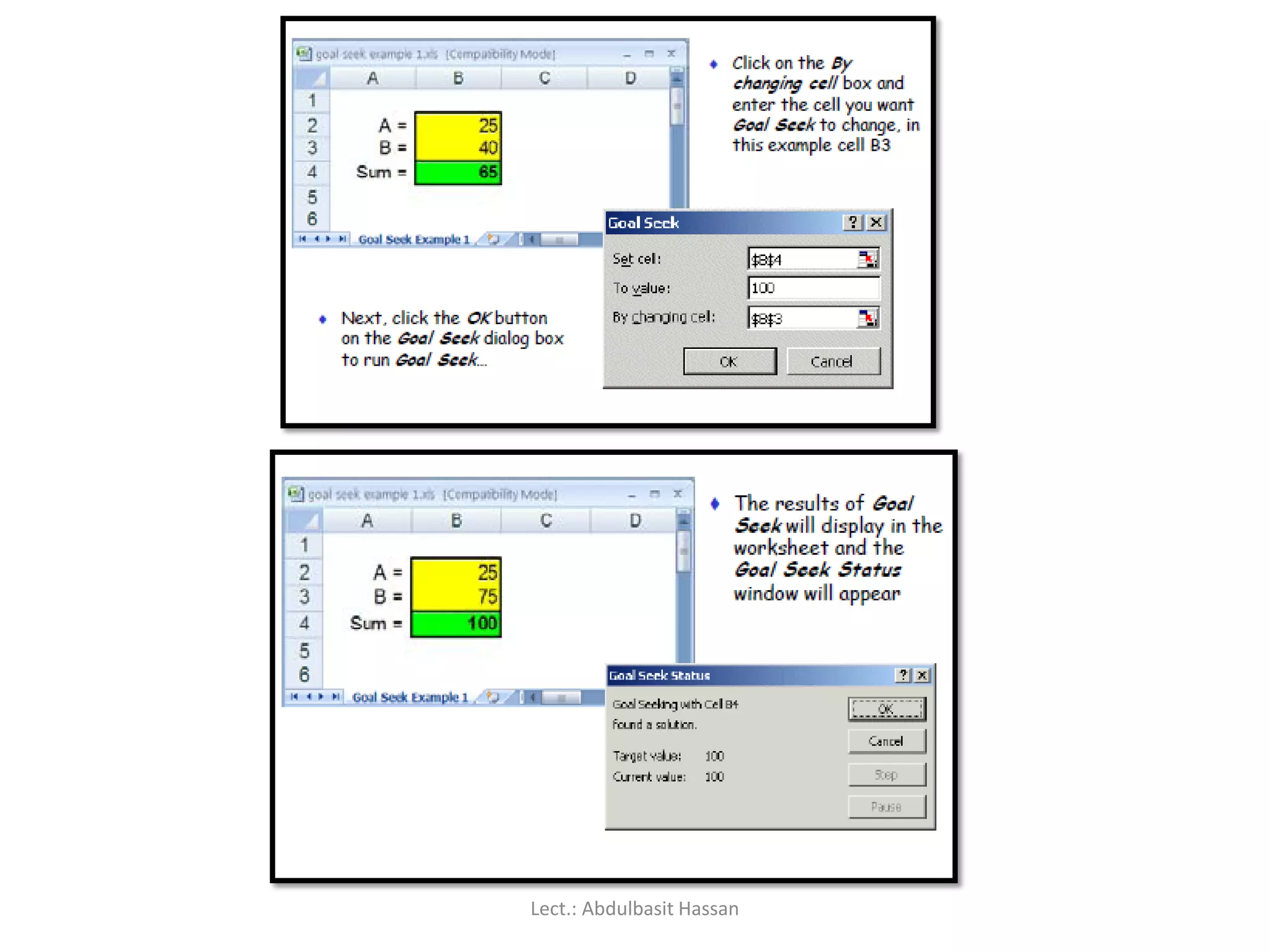
Example : Wewill use Goal Seek to find a number to make the sum
equal to 100:
B2 = 25; B3 = 40; B4 = SUM(B2:B3)
Goal Seek will change the value in cell B3 incrementally until the sum
in B4 equals 100.
Lect.: Abdulbasit Hassan
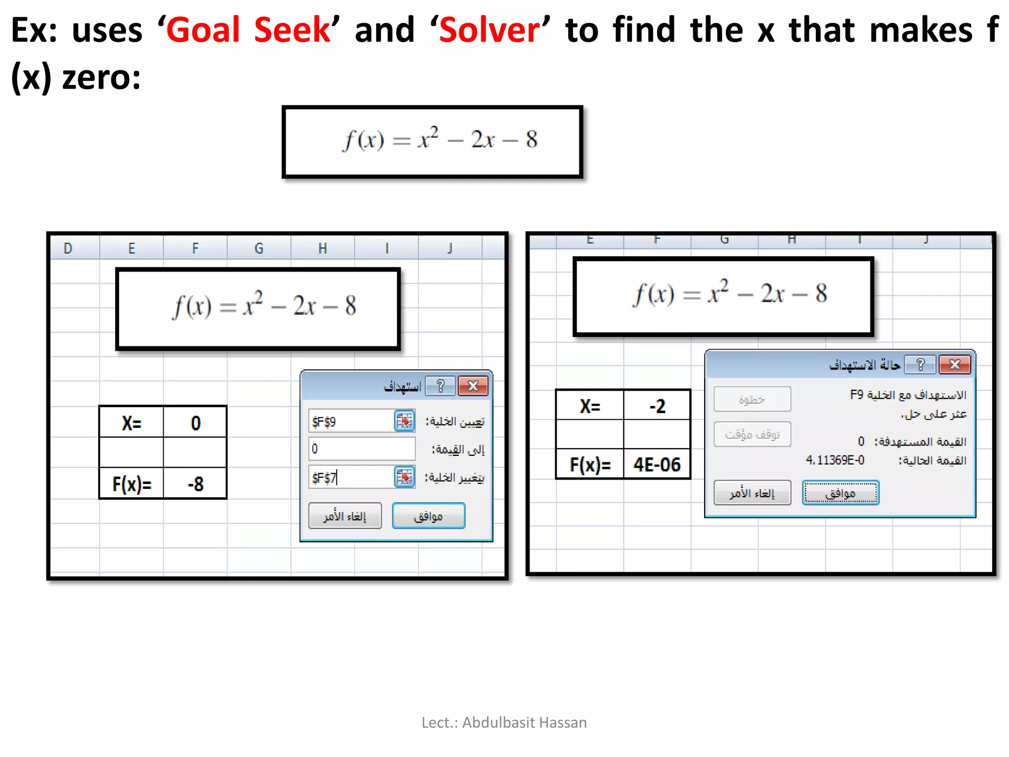
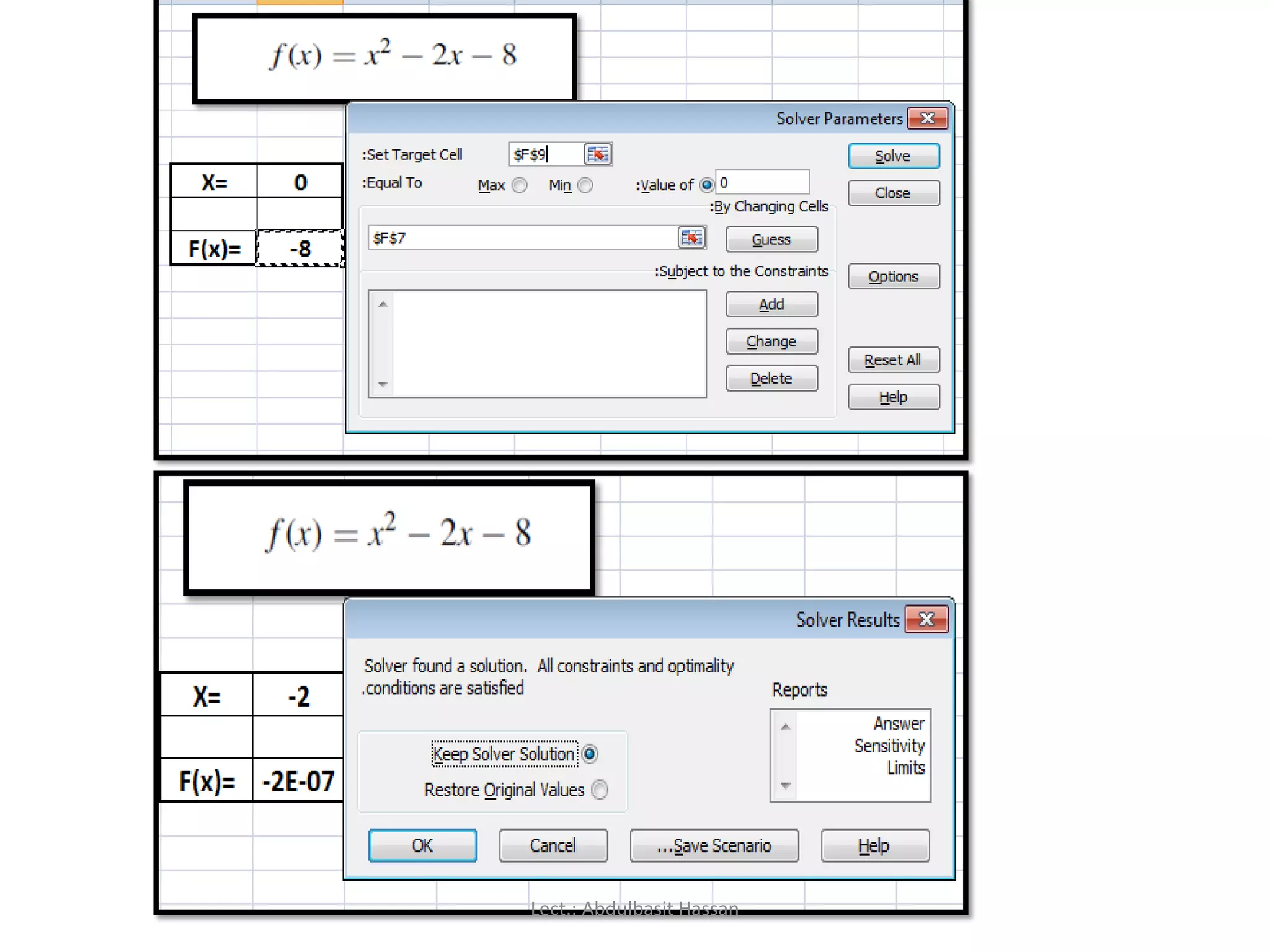
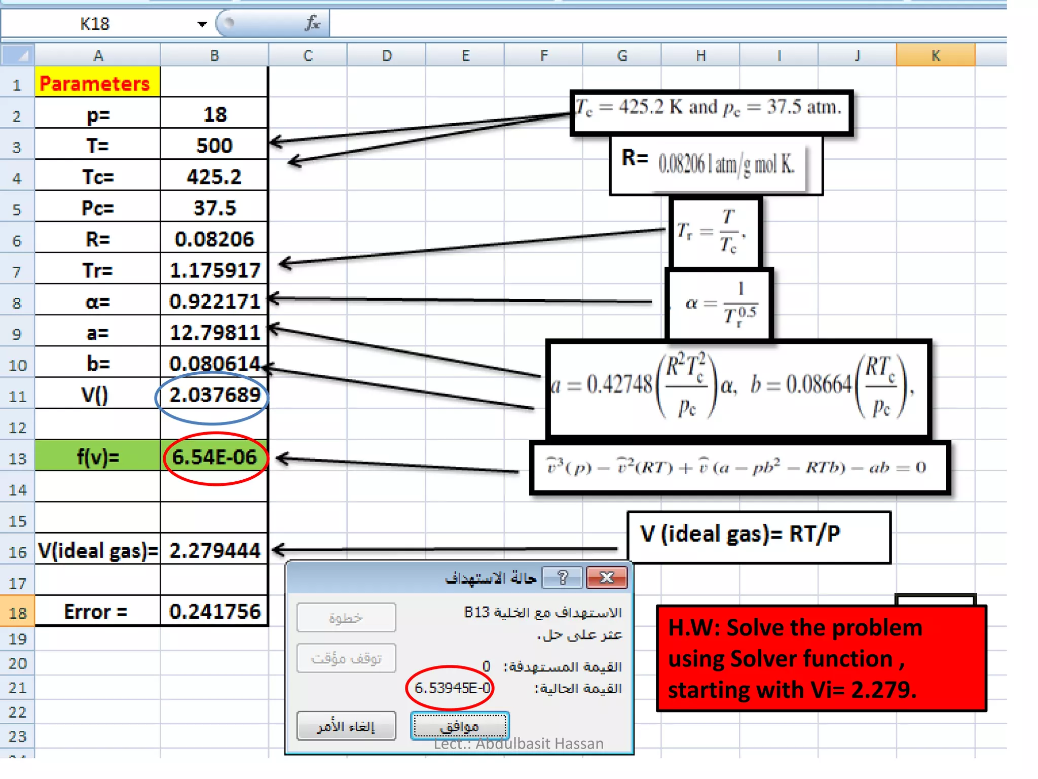
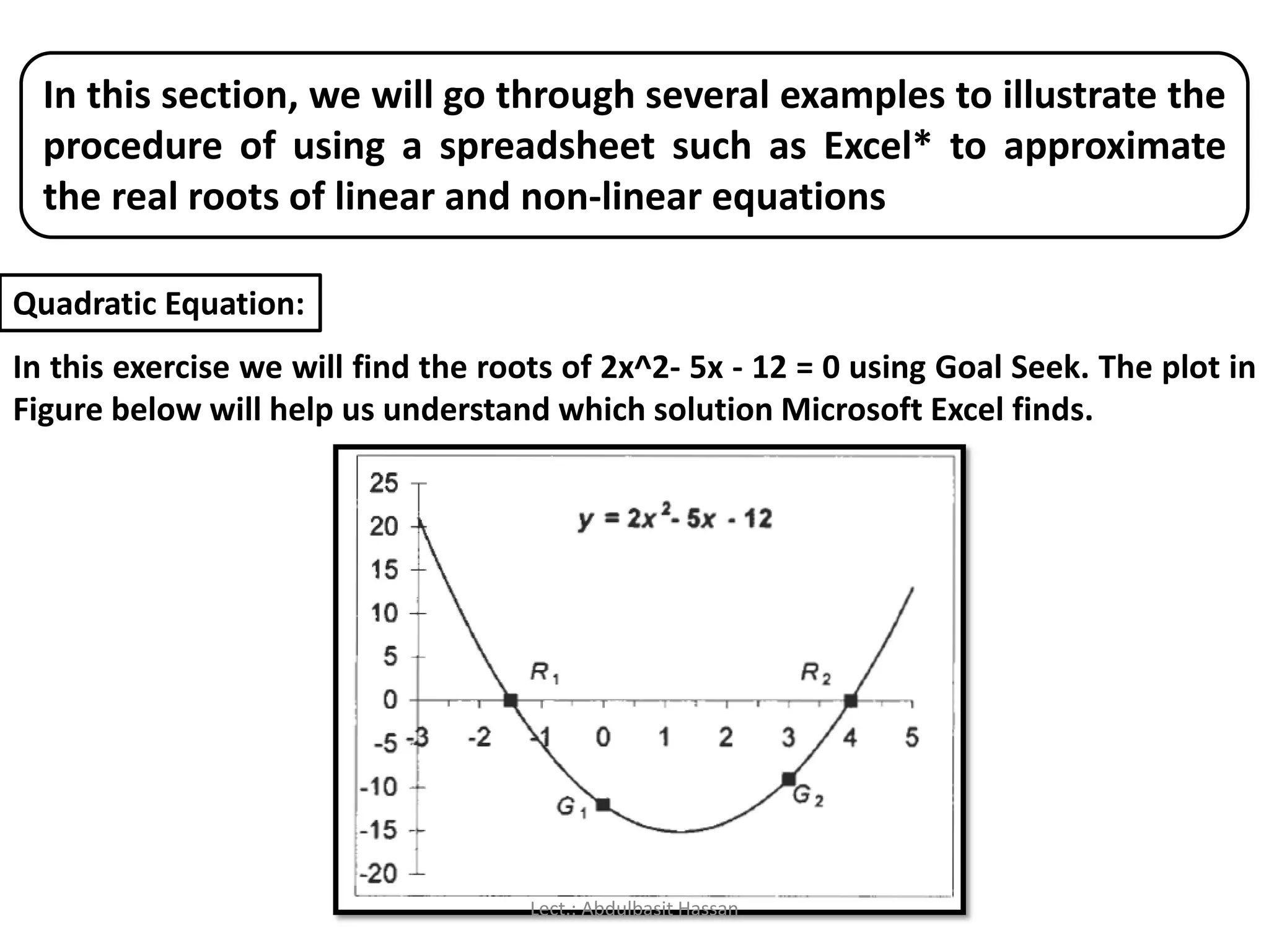
In this section,we will go through several examples to illustrate the
procedure of using a spreadsheet such as Excel* to approximate
the real roots of linear and non-linear equations
Quadratic Equation:
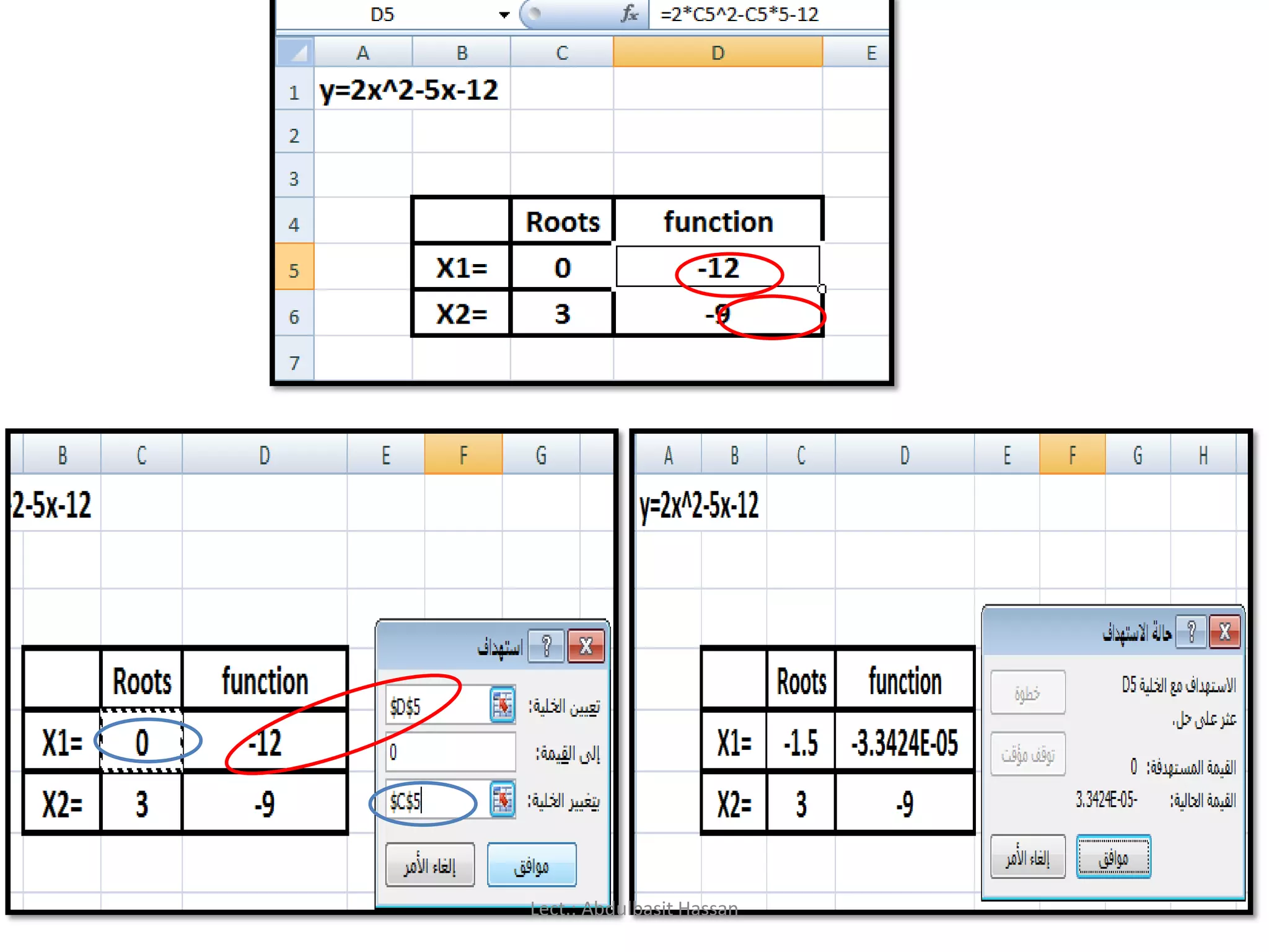
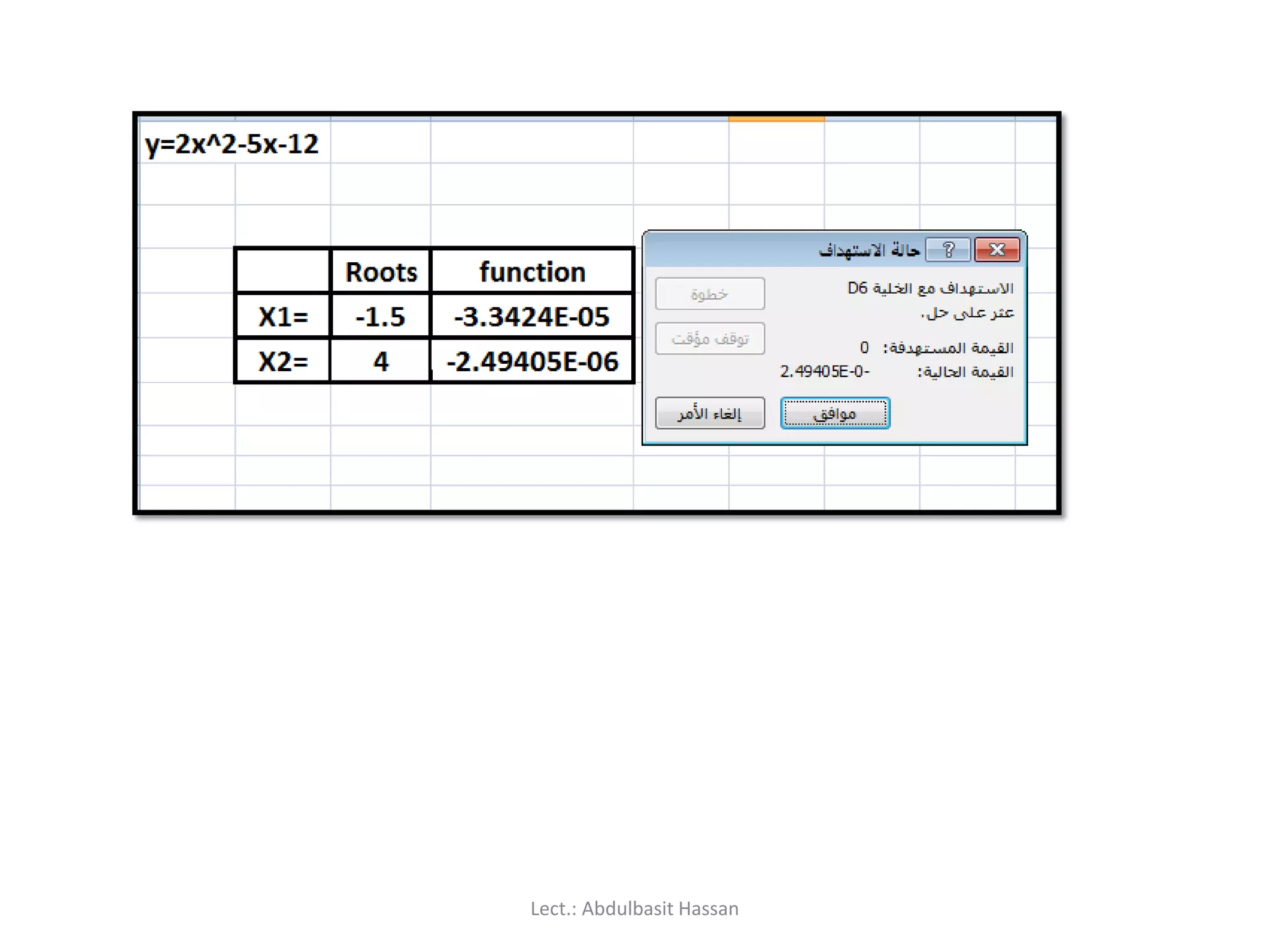
In this exercise we will find the roots of 2x^2- 5x - 12 = 0 using Goal Seek. The plot in
Figure below will help us understand which solution Microsoft Excel finds.
Lect.: Abdulbasit Hassan
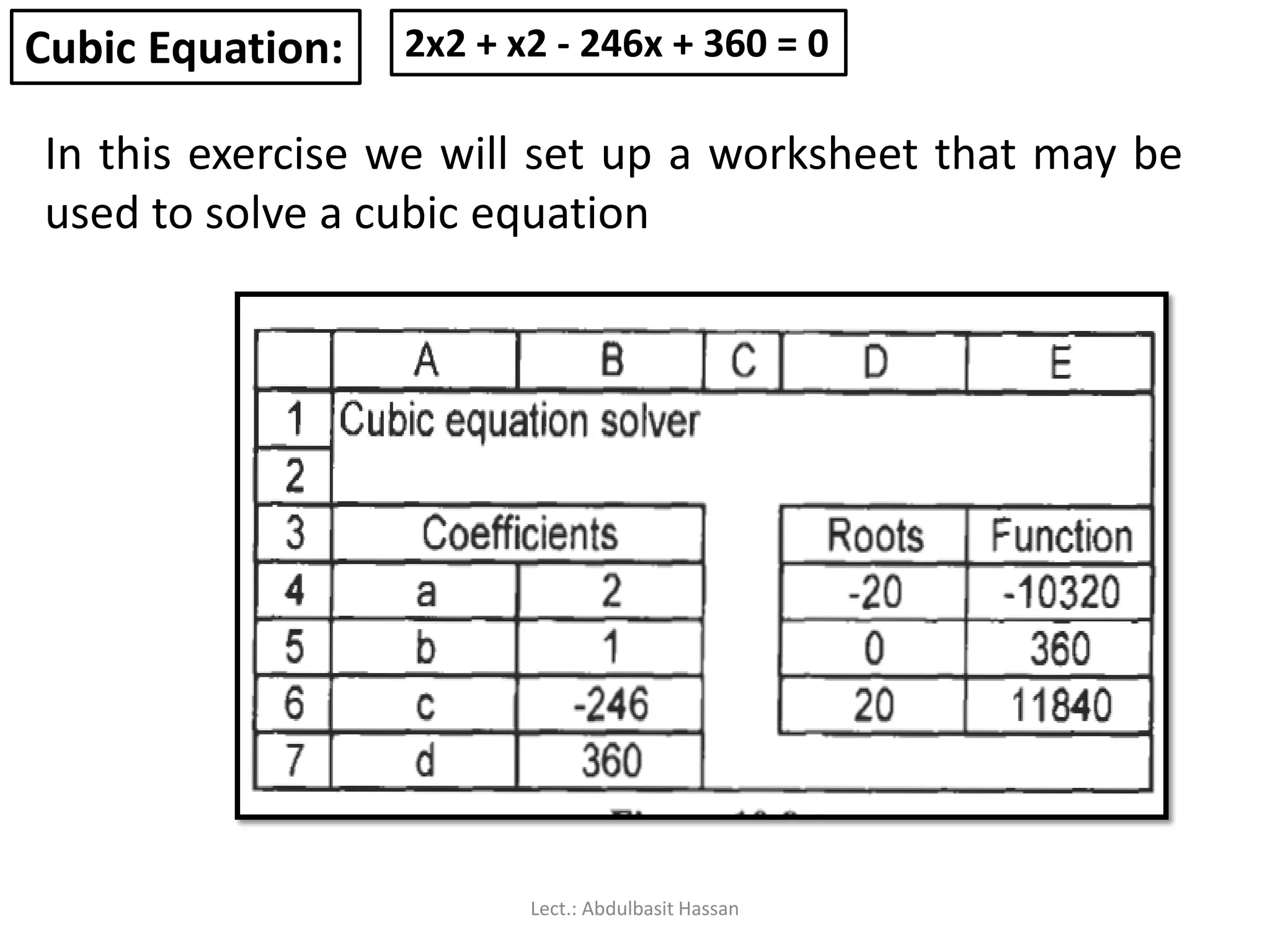
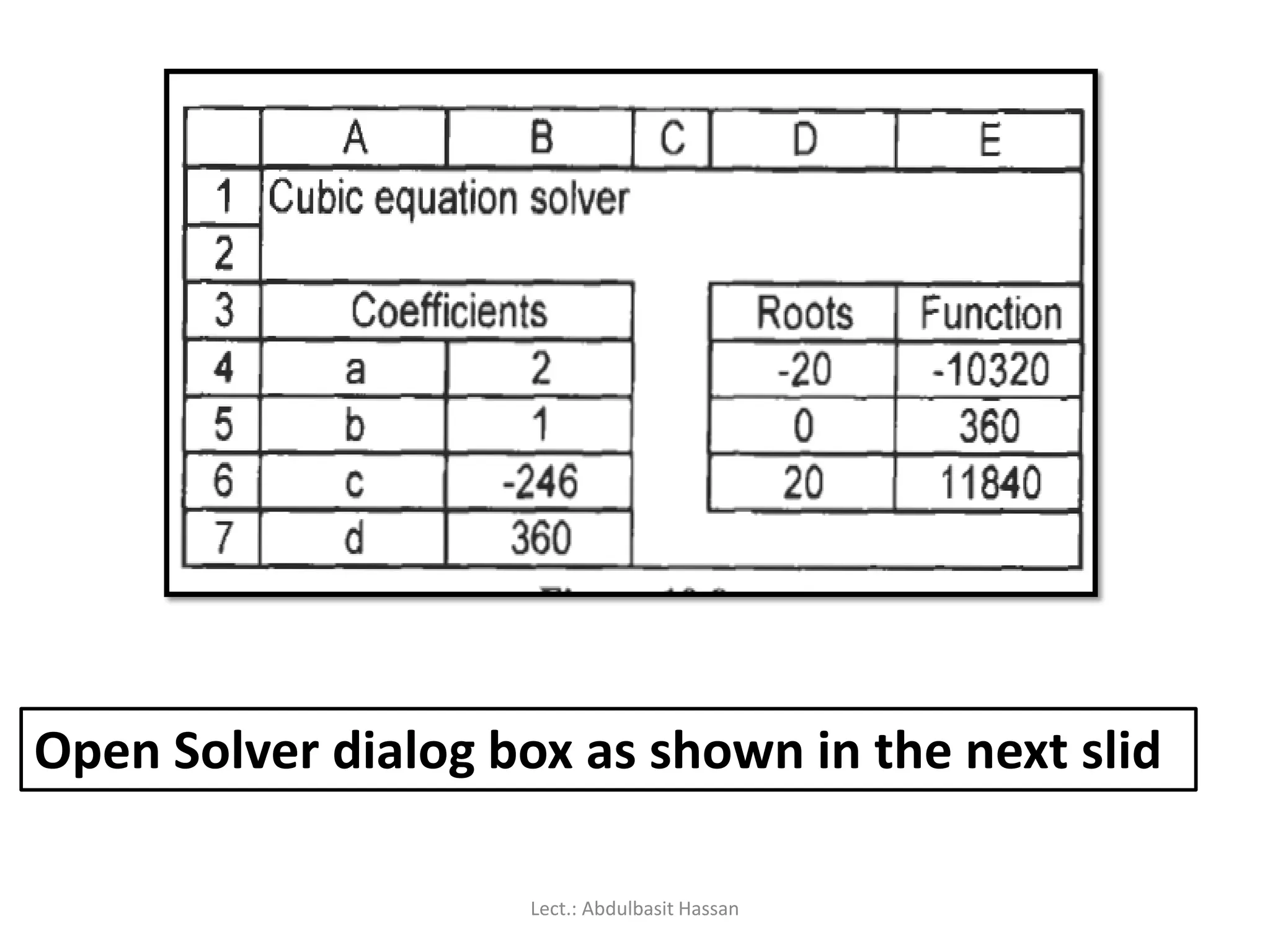
Cubic Equation: 2x2+ x2 - 246x + 360 = 0
In this exercise we will set up a worksheet that may be
used to solve a cubic equation
Lect.: Abdulbasit Hassan
219.
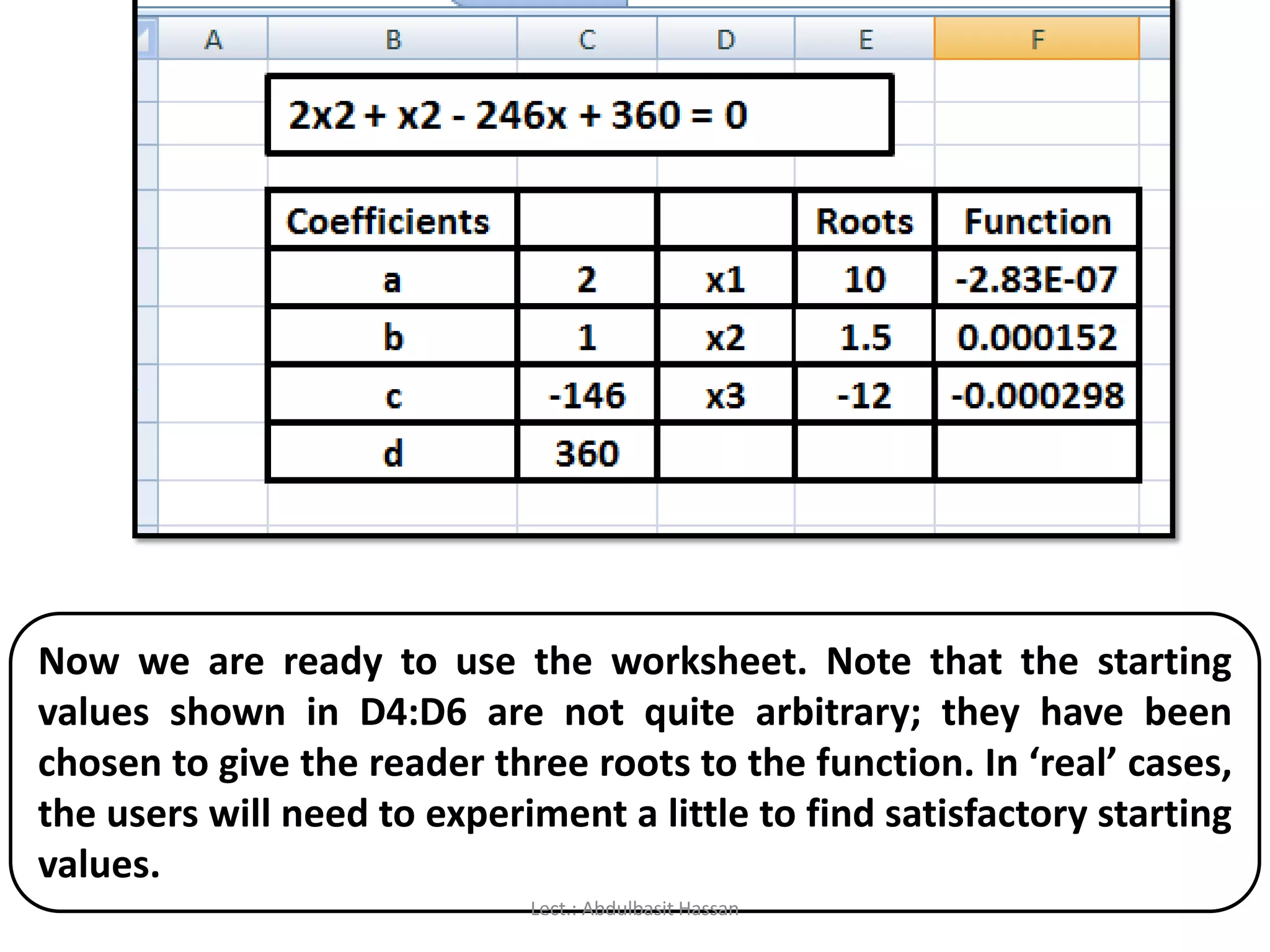
Now we areready to use the worksheet. Note that the starting
values shown in D4:D6 are not quite arbitrary; they have been
chosen to give the reader three roots to the function. In ‘real’ cases,
the users will need to experiment a little to find satisfactory starting
values.
Lect.: Abdulbasit Hassan
220.
Roots of aCubic Equation with
Solver
Lect.: Abdulbasit Hassan
221.
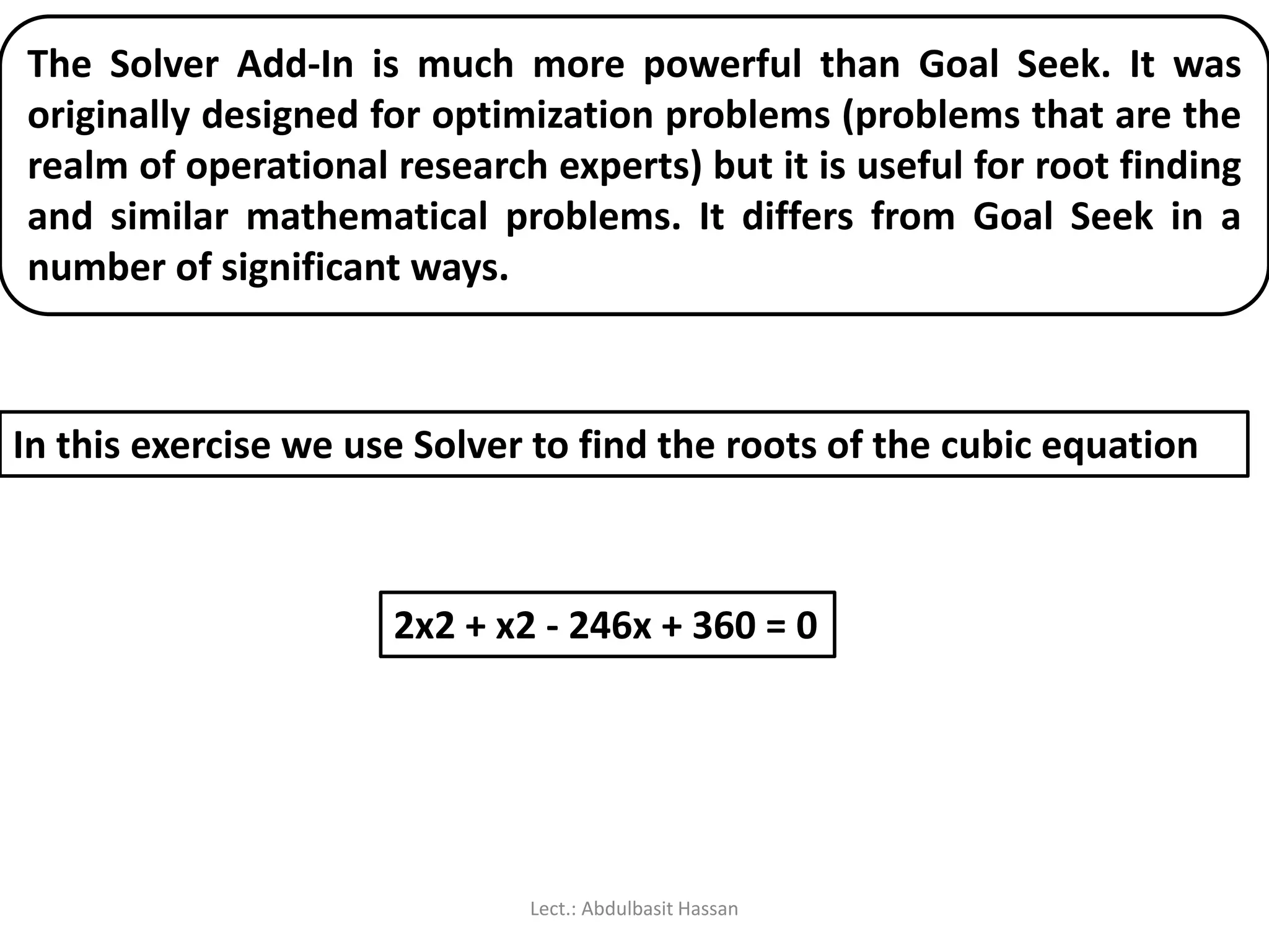
The Solver Add-Inis much more powerful than Goal Seek. It was
originally designed for optimization problems (problems that are the
realm of operational research experts) but it is useful for root finding
and similar mathematical problems. It differs from Goal Seek in a
number of significant ways.
2x2 + x2 - 246x + 360 = 0
In this exercise we use Solver to find the roots of the cubic equation
Lect.: Abdulbasit Hassan
222.
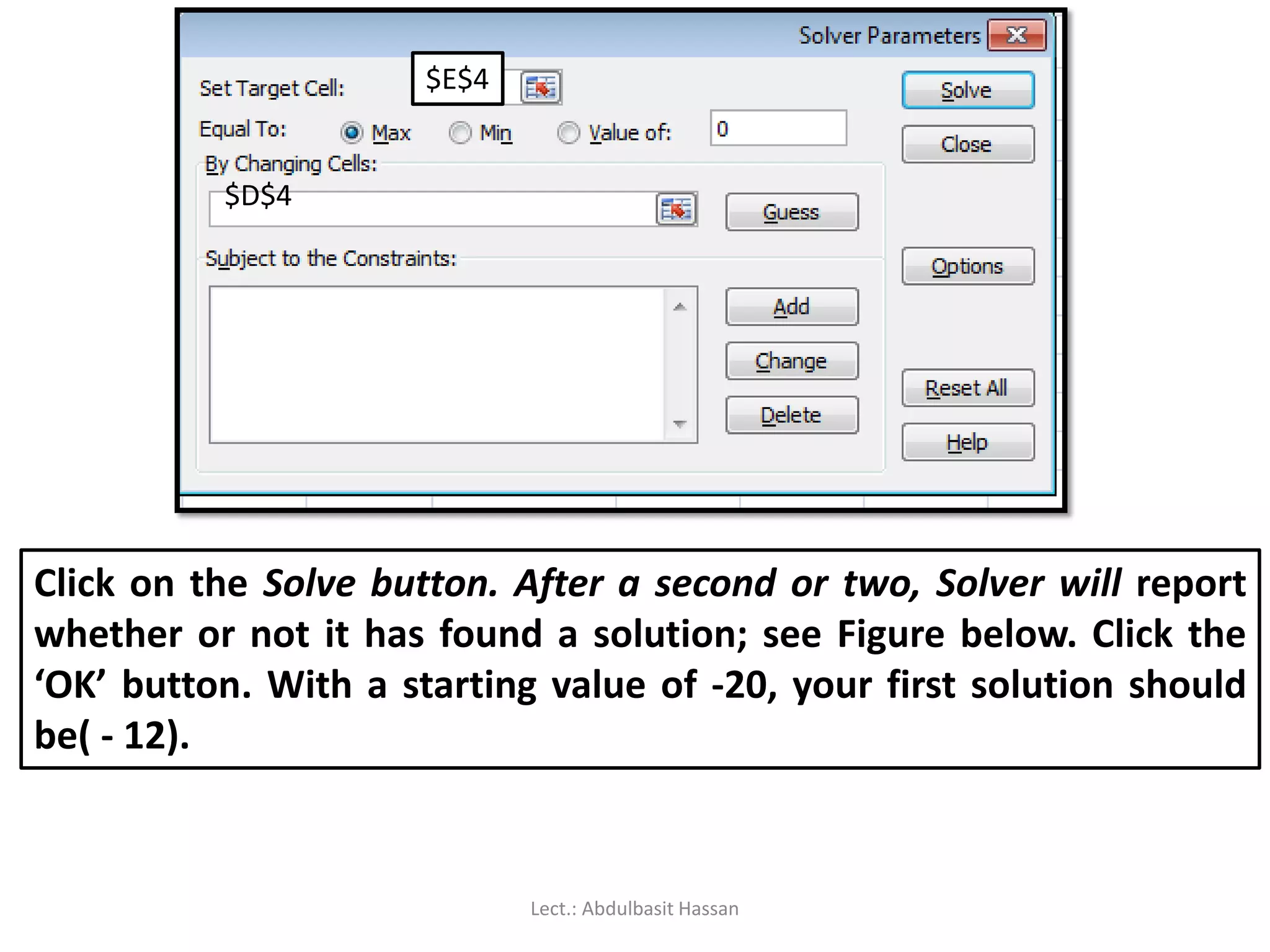
Open Solver dialogbox as shown in the next slid
Lect.: Abdulbasit Hassan
223.
$D$4
$E$4
Click on theSolve button. After a second or two, Solver will report
whether or not it has found a solution; see Figure below. Click the
‘OK’ button. With a starting value of -20, your first solution should
be( - 12).
Lect.: Abdulbasit Hassan
224.
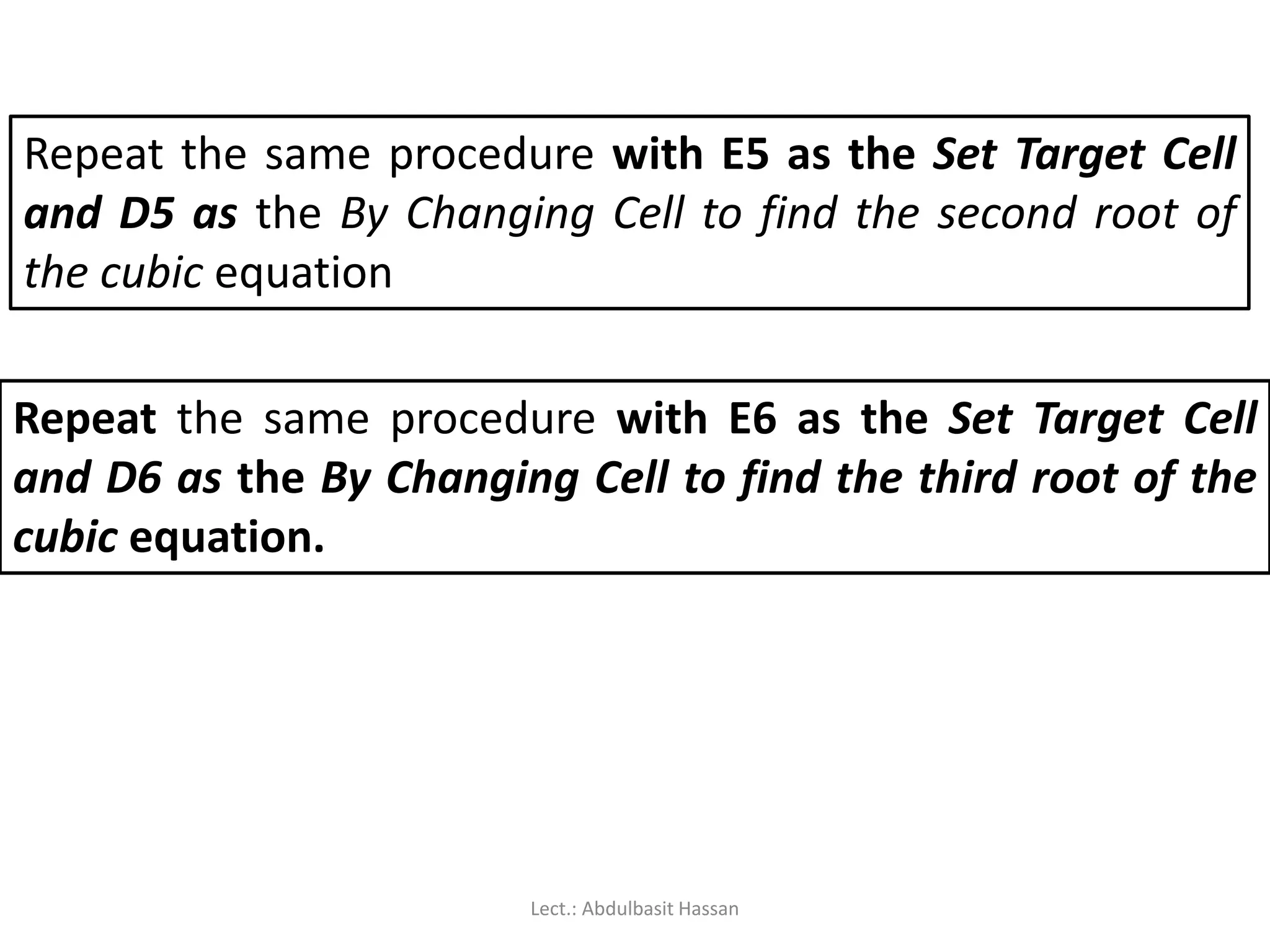
Repeat the sameprocedure with E5 as the Set Target Cell
and D5 as the By Changing Cell to find the second root of
the cubic equation
Repeat the same procedure with E6 as the Set Target Cell
and D6 as the By Changing Cell to find the third root of the
cubic equation.
Lect.: Abdulbasit Hassan
225.
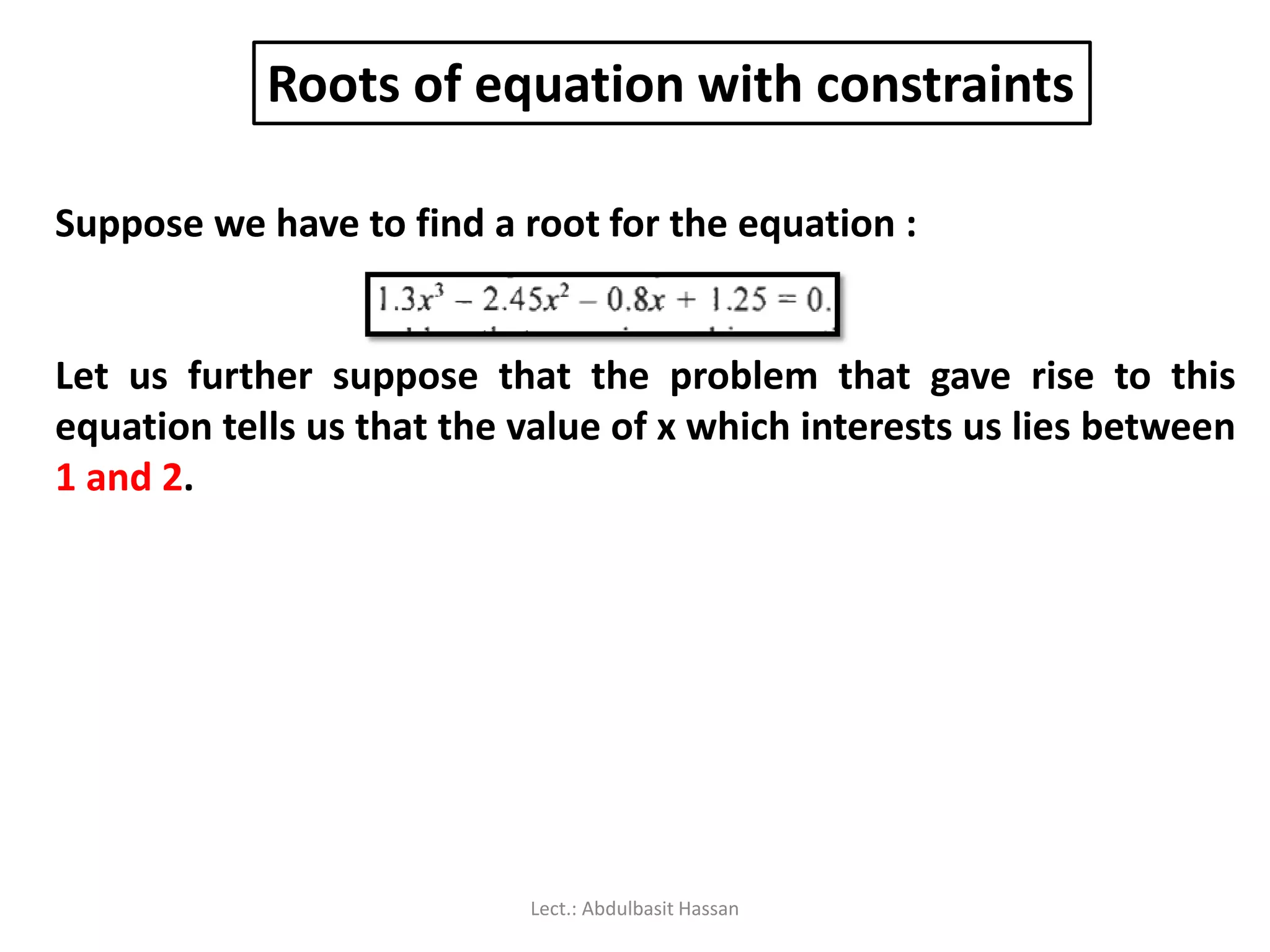
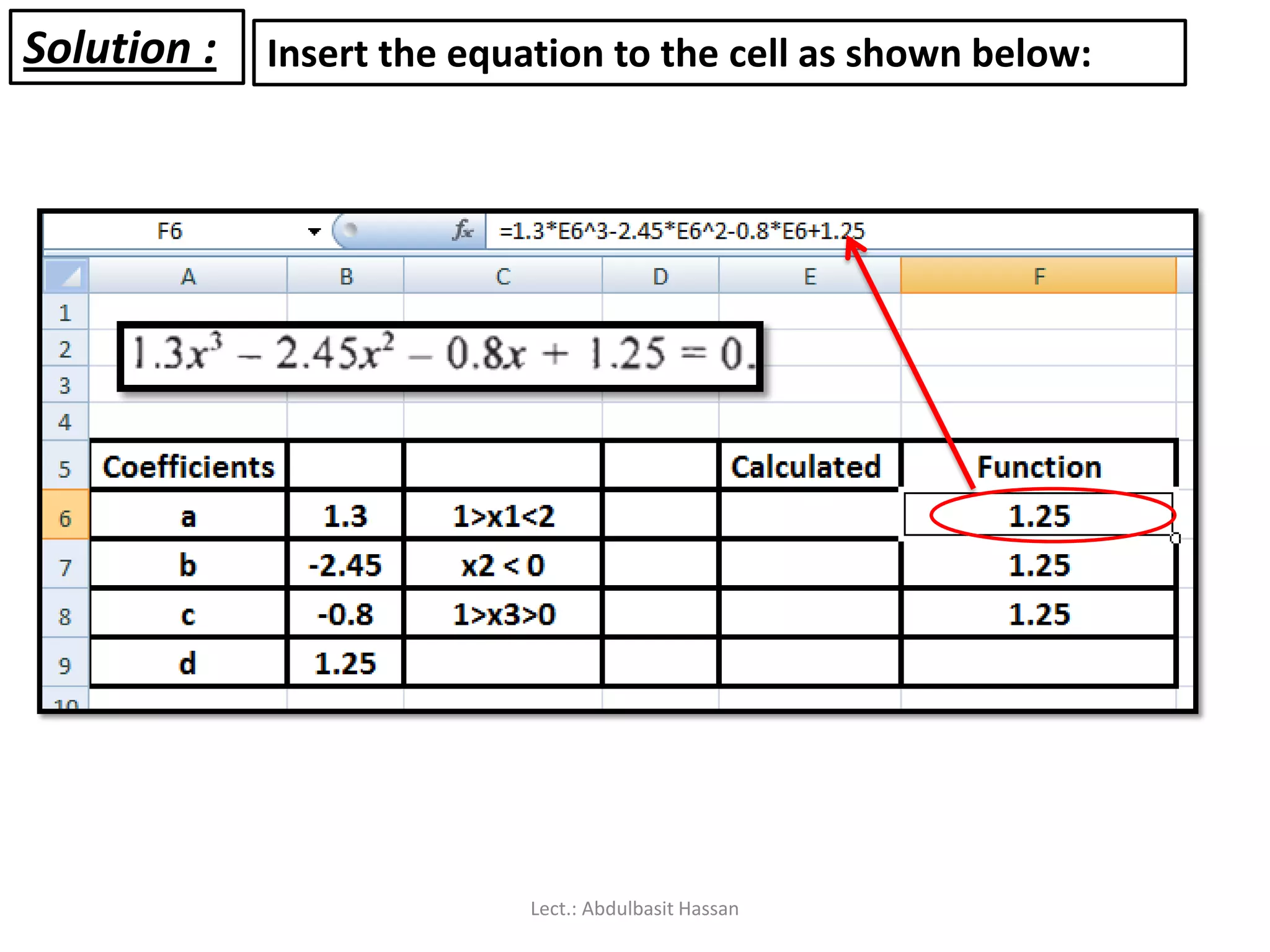
Roots of equationwith constraints
Suppose we have to find a root for the equation :
Let us further suppose that the problem that gave rise to this
equation tells us that the value of x which interests us lies between
1 and 2.
Lect.: Abdulbasit Hassan
226.
Solution : Insertthe equation to the cell as shown below:
Lect.: Abdulbasit Hassan
227.
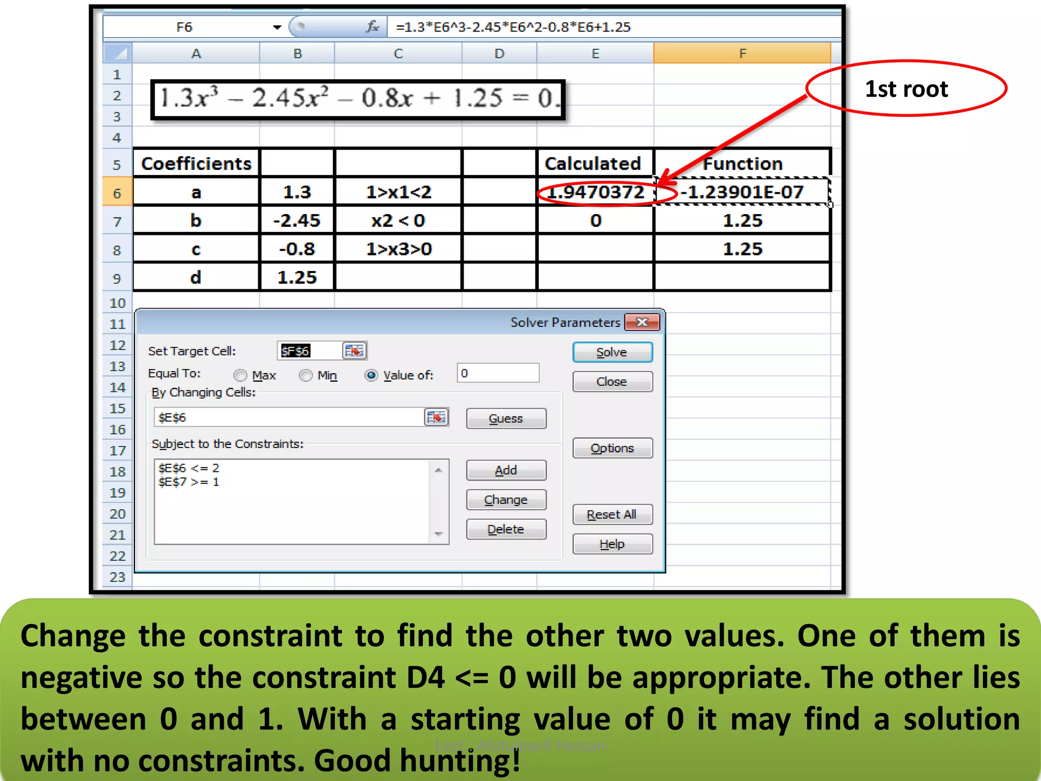
1st root
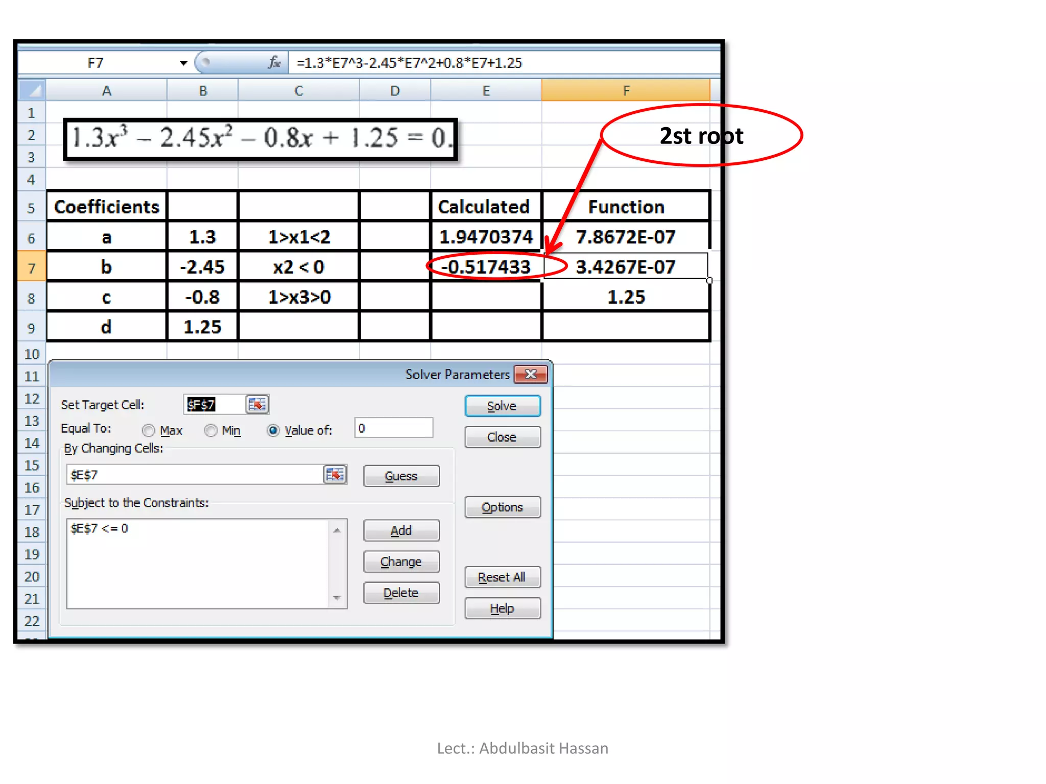
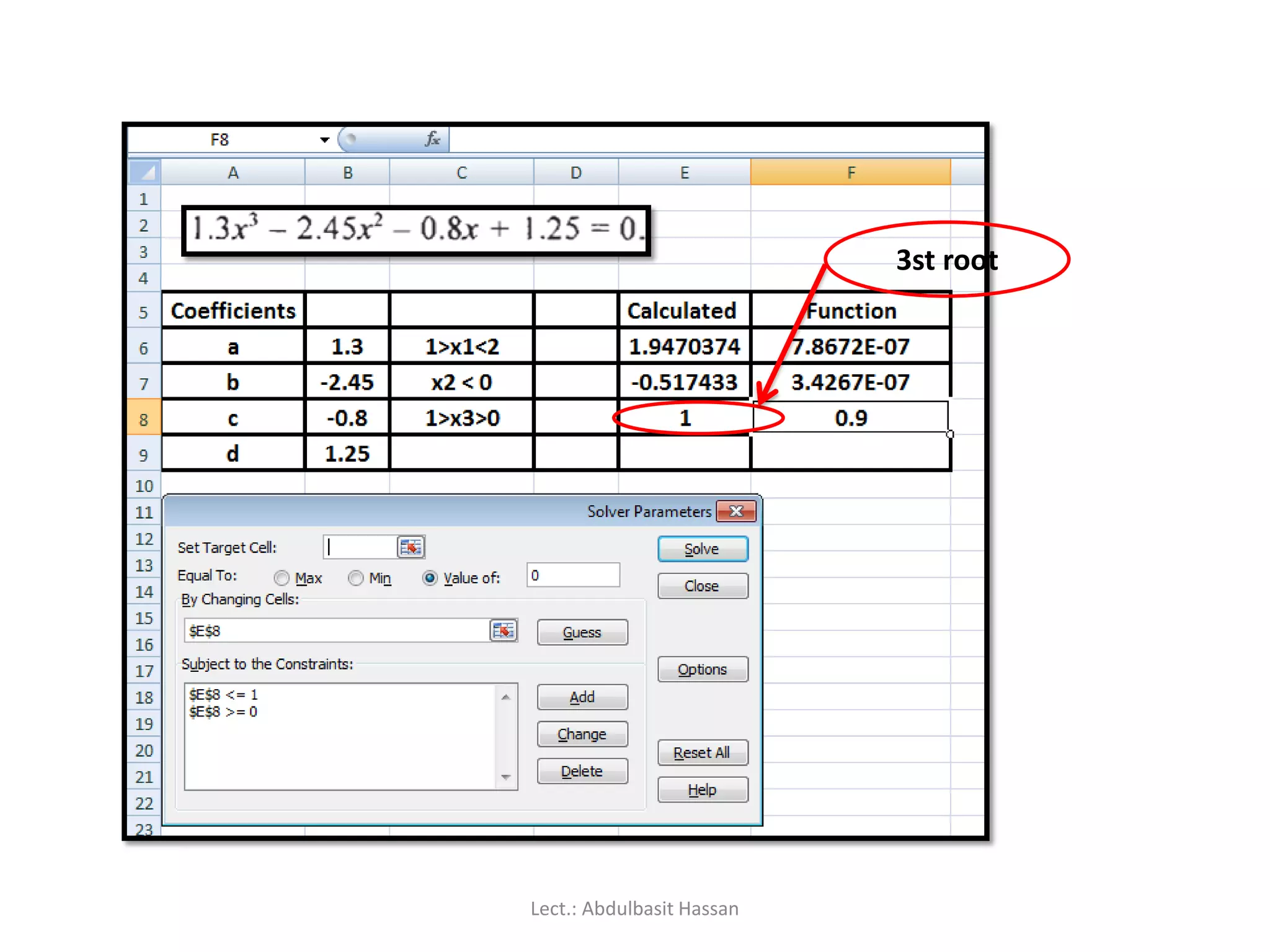
Change theconstraint to find the other two values. One of them is
negative so the constraint D4 <= 0 will be appropriate. The other lies
between 0 and 1. With a starting value of 0 it may find a solution
with no constraints. Good hunting!
Lect.: Abdulbasit Hassan
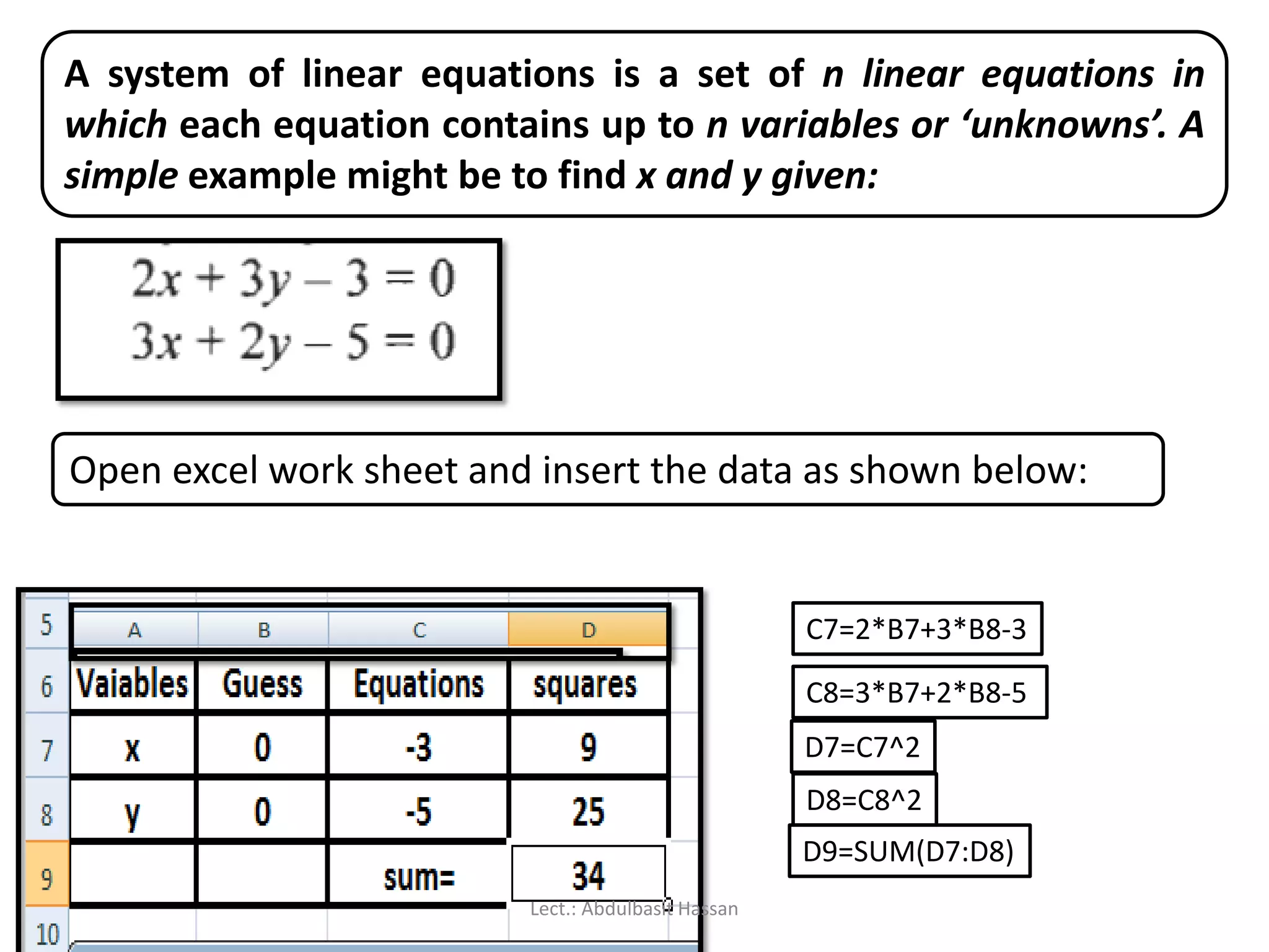
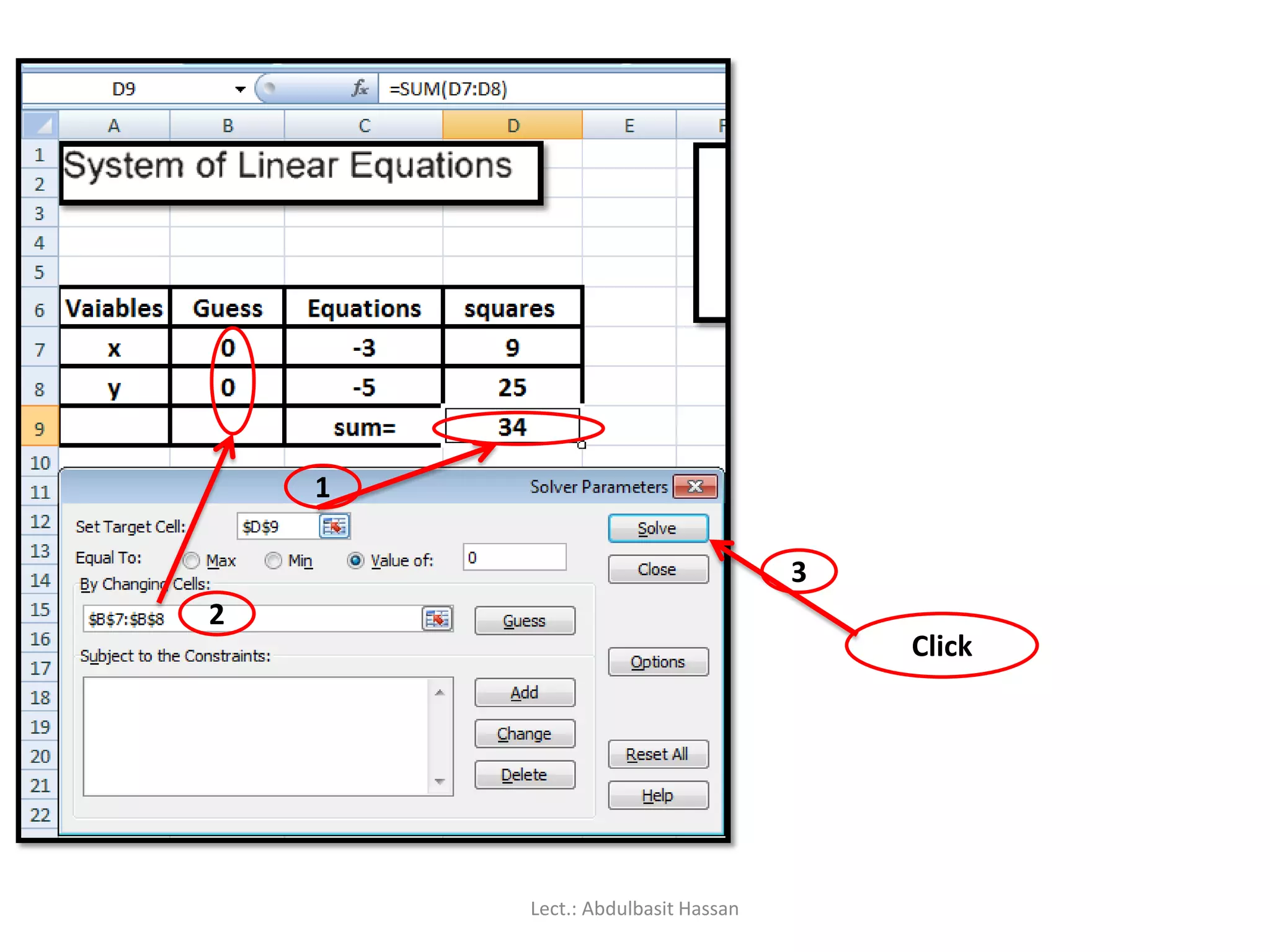
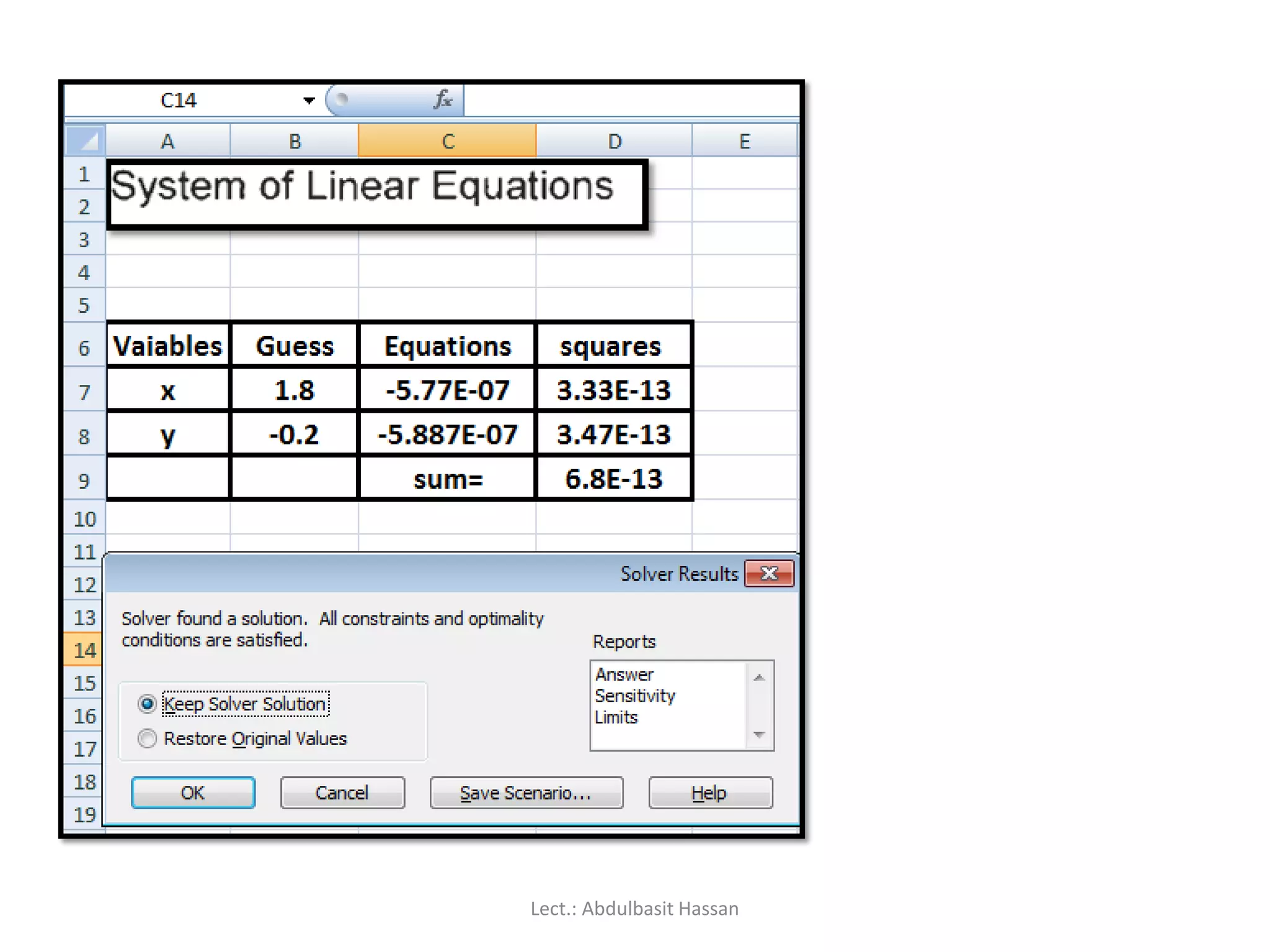
A system oflinear equations is a set of n linear equations in
which each equation contains up to n variables or ‘unknowns’. A
simple example might be to find x and y given:
Open excel work sheet and insert the data as shown below:
C7=2*B7+3*B8-3
C8=3*B7+2*B8-5
D7=C7^2
D8=C8^2
D9=SUM(D7:D8)
Lect.: Abdulbasit Hassan
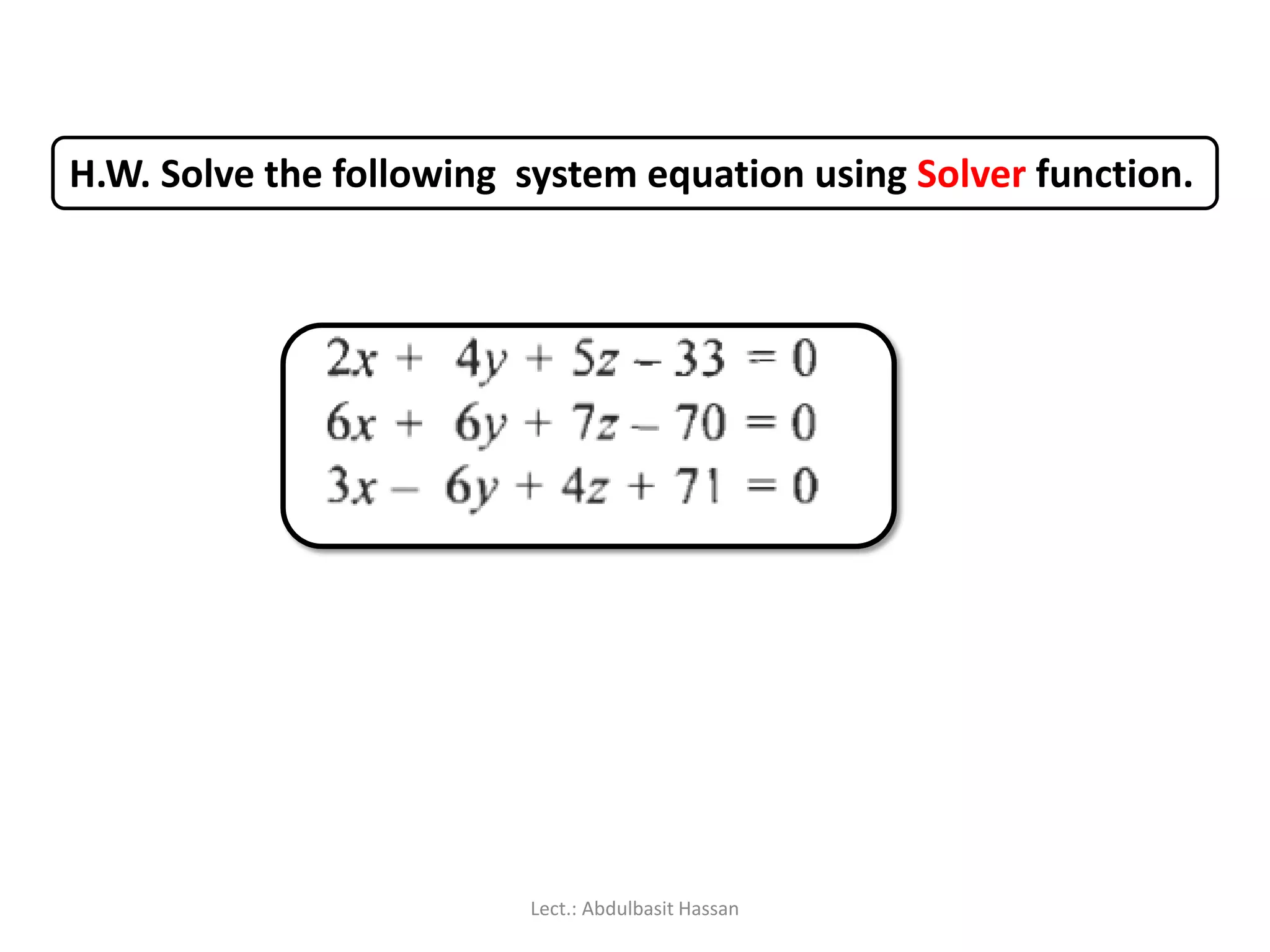
H.W. Solve thefollowing system equation using Solver function.
Lect.: Abdulbasit Hassan
235.
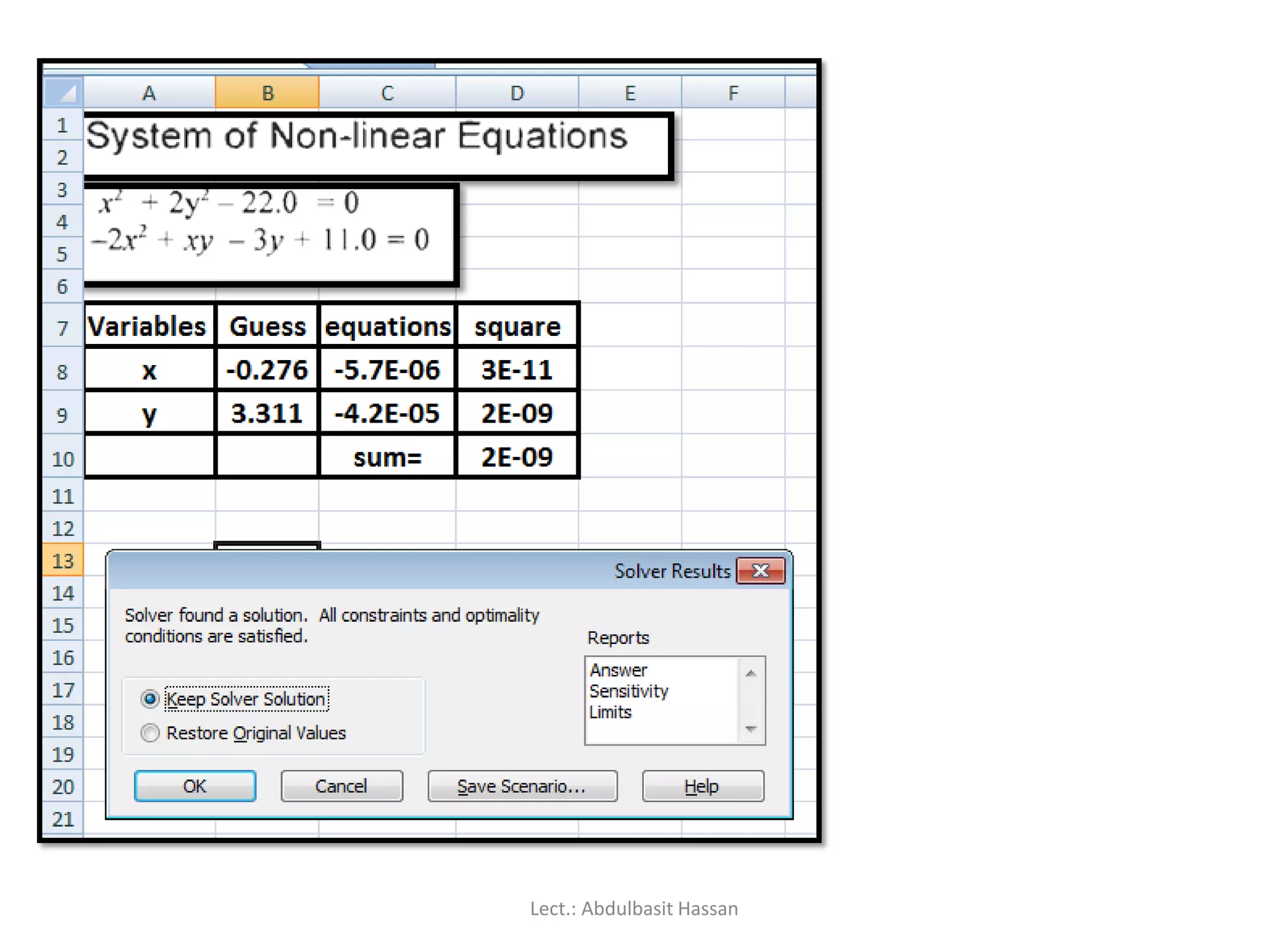
Non - linearSimultaneous
Equations Solver
Lect.: Abdulbasit Hassan
236.
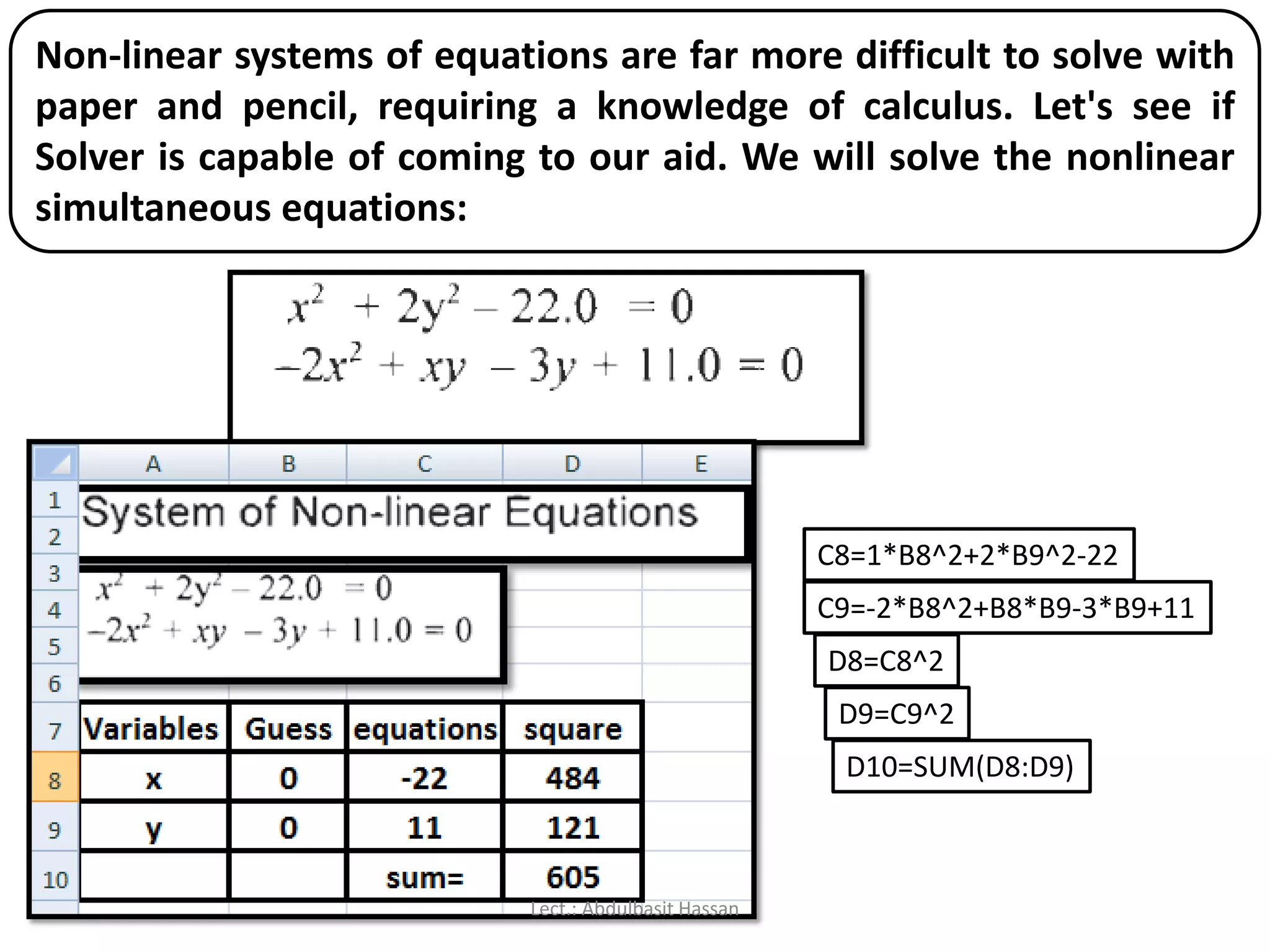
Non-linear systems ofequations are far more difficult to solve with
paper and pencil, requiring a knowledge of calculus. Let's see if
Solver is capable of coming to our aid. We will solve the nonlinear
simultaneous equations:
C8=1*B8^2+2*B9^2-22
C9=-2*B8^2+B8*B9-3*B9+11
D8=C8^2
D9=C9^2
D10=SUM(D8:D9)
Lect.: Abdulbasit Hassan
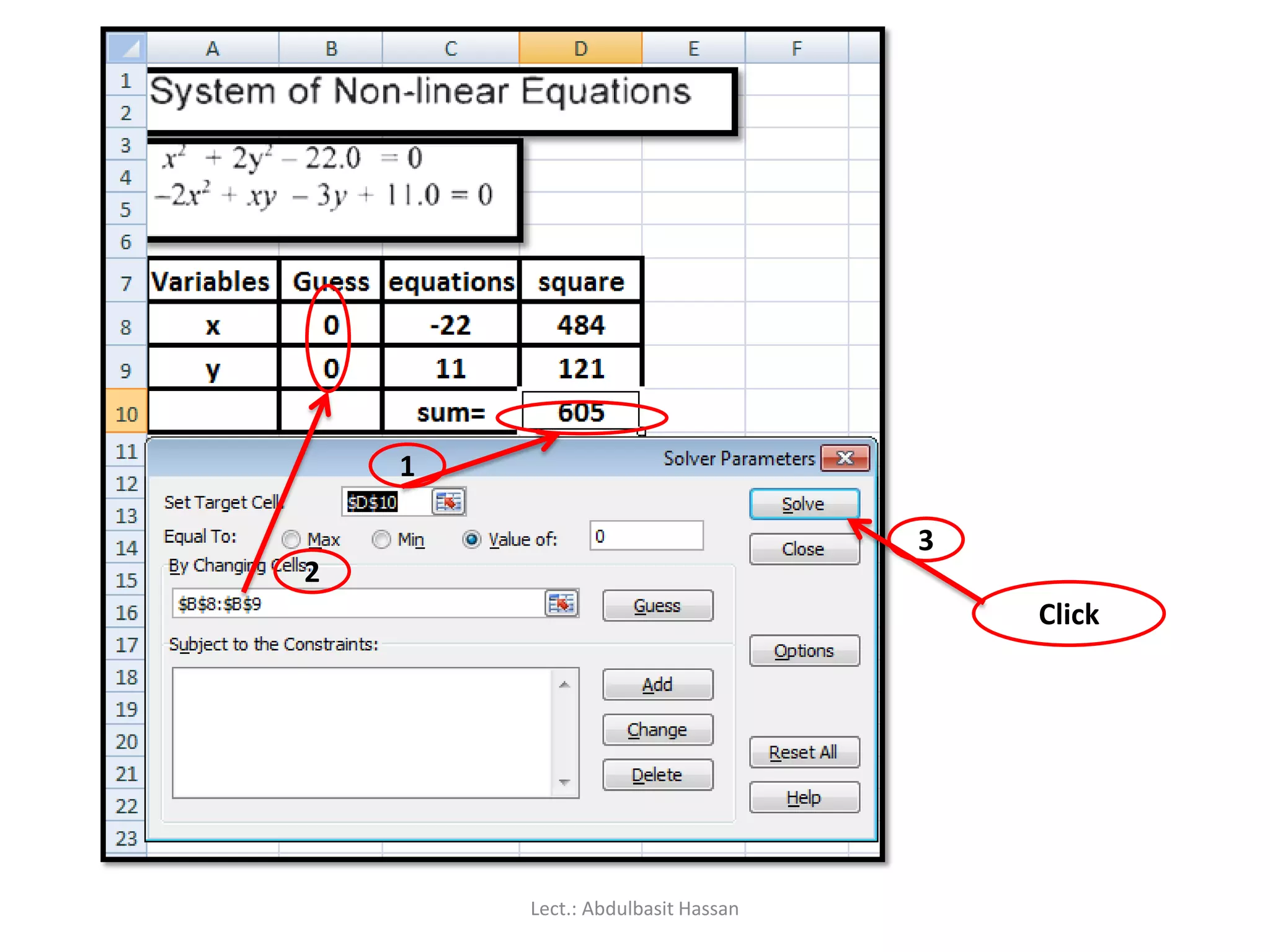
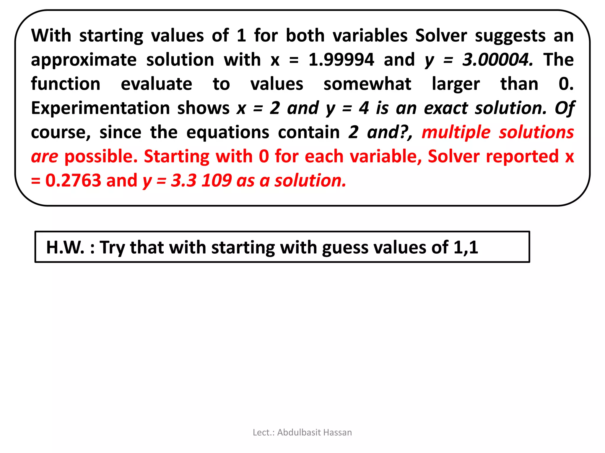
With starting valuesof 1 for both variables Solver suggests an
approximate solution with x = 1.99994 and y = 3.00004. The
function evaluate to values somewhat larger than 0.
Experimentation shows x = 2 and y = 4 is an exact solution. Of
course, since the equations contain 2 and?, multiple solutions
are possible. Starting with 0 for each variable, Solver reported x
= 0.2763 and y = 3.3 109 as a solution.
H.W. : Try that with starting with guess values of 1,1
Lect.: Abdulbasit Hassan
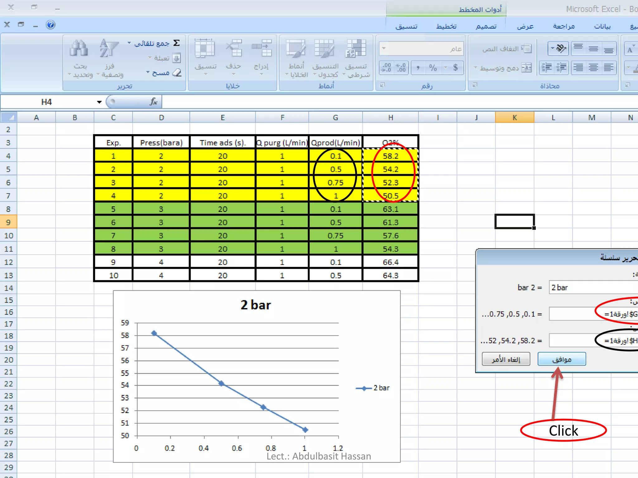
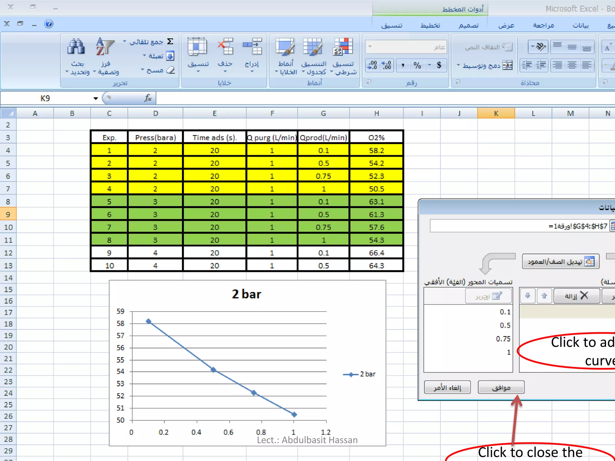
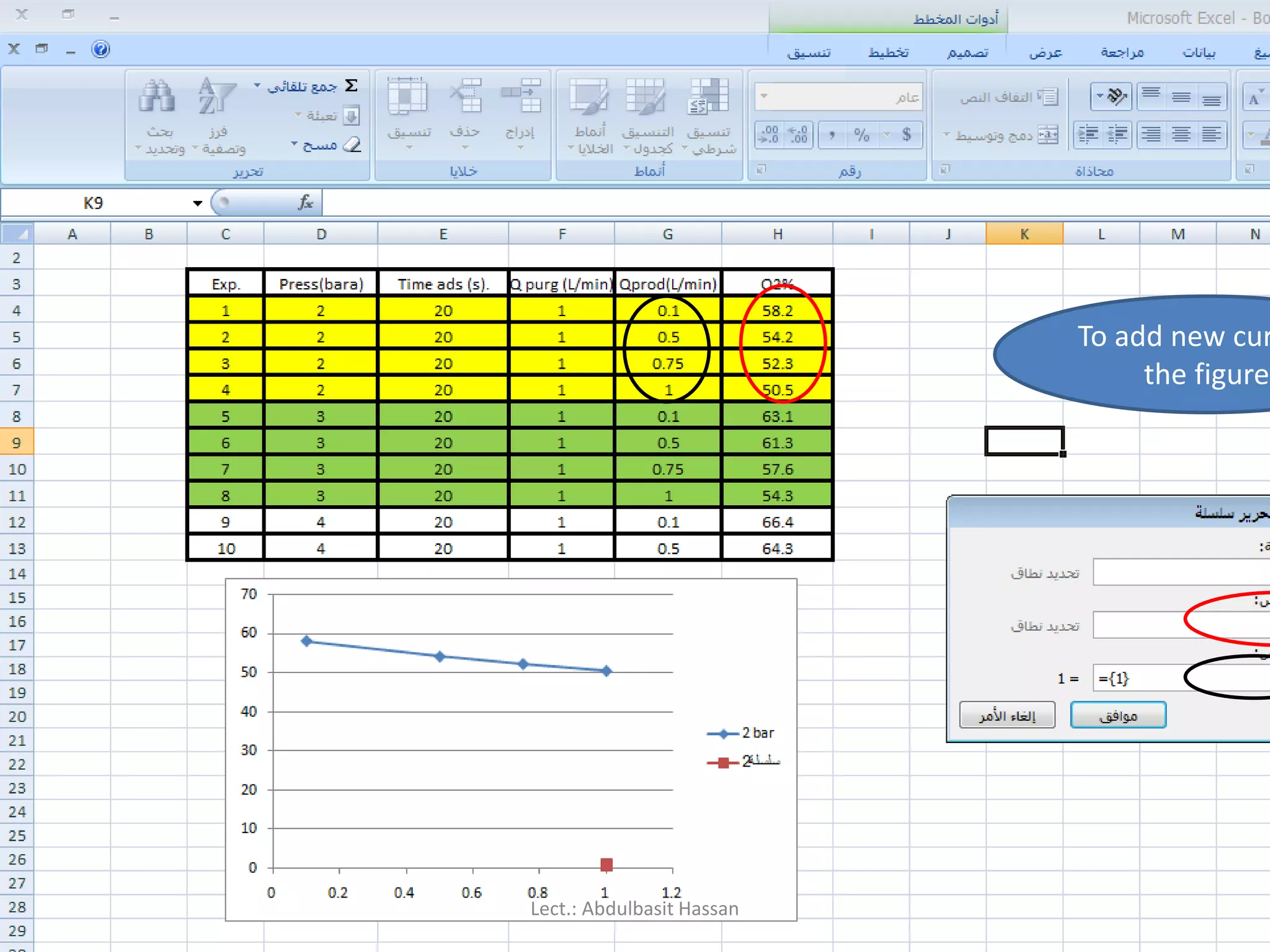
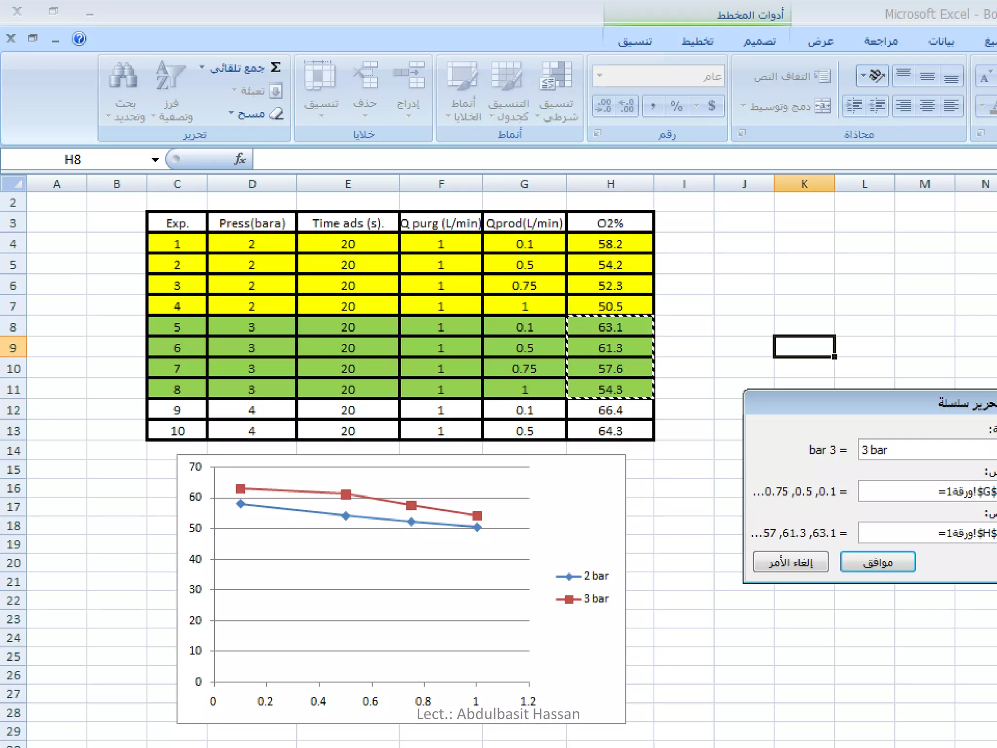
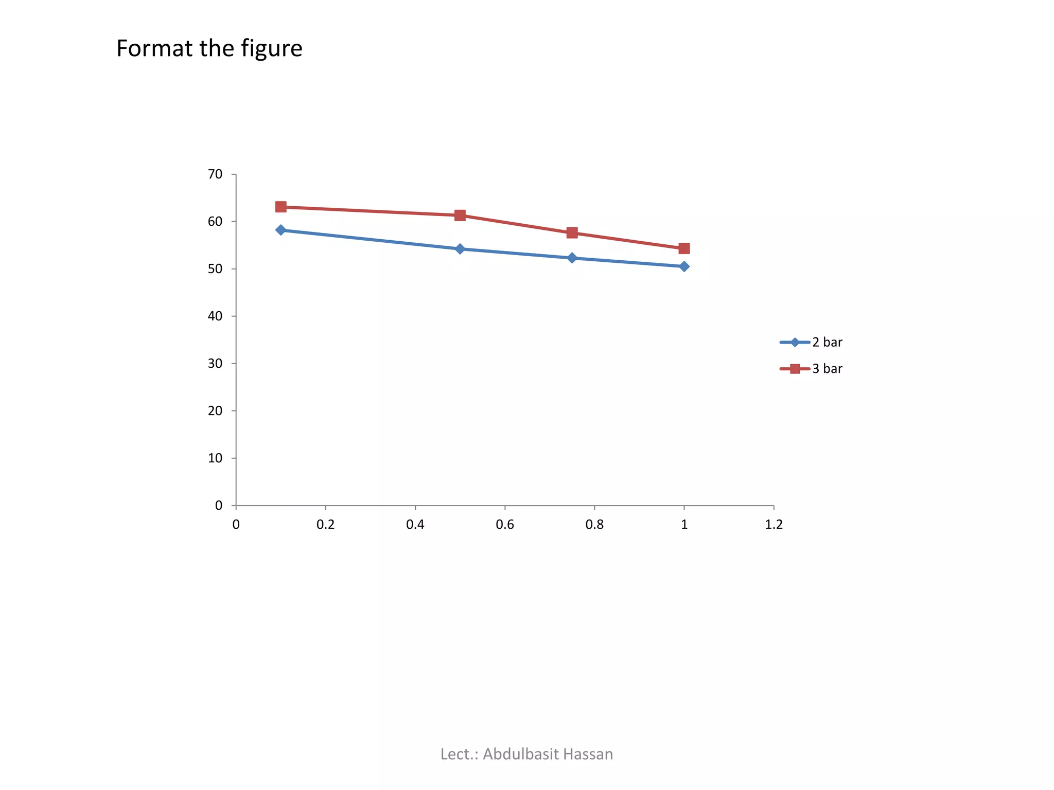
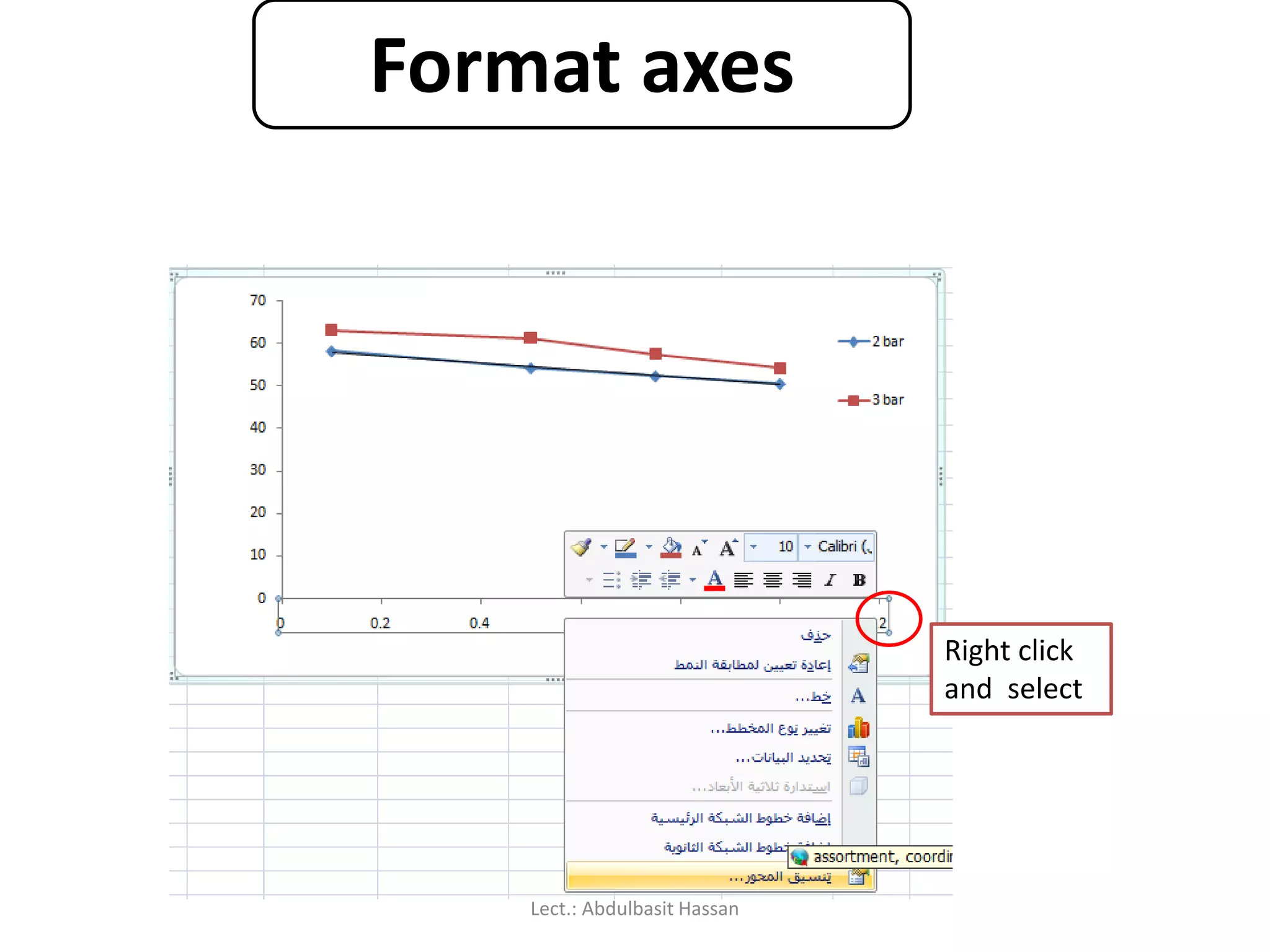
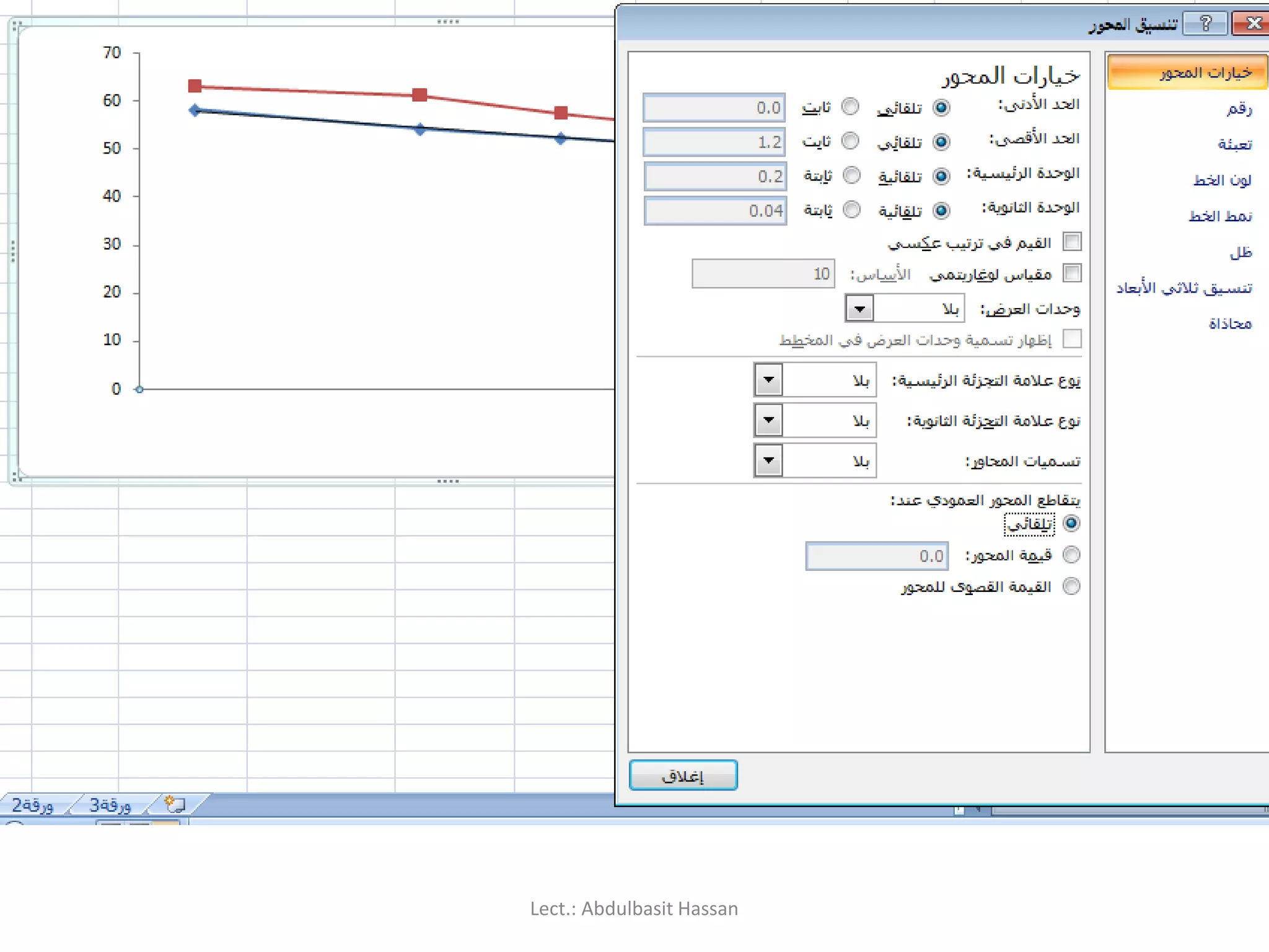
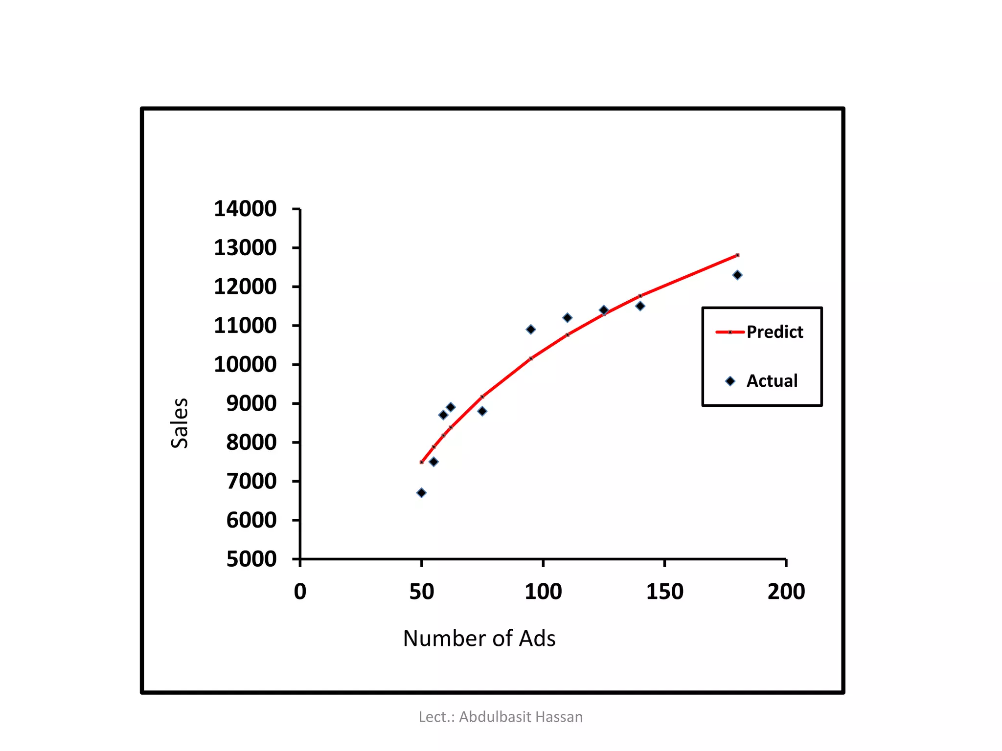
Description: We willfocus on Excel features for graphs
and charts. We will discuss multiple axes, formatting data,
choosing chart type, adding notes and images, and
customizing your charts. We will discuss how to export
charts to other formats including Word, PowerPoint and
PDF.
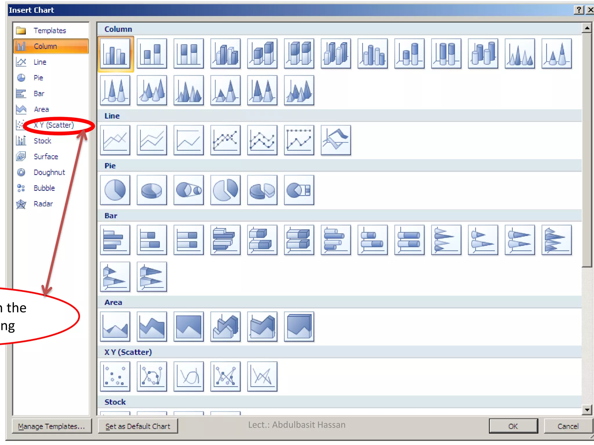
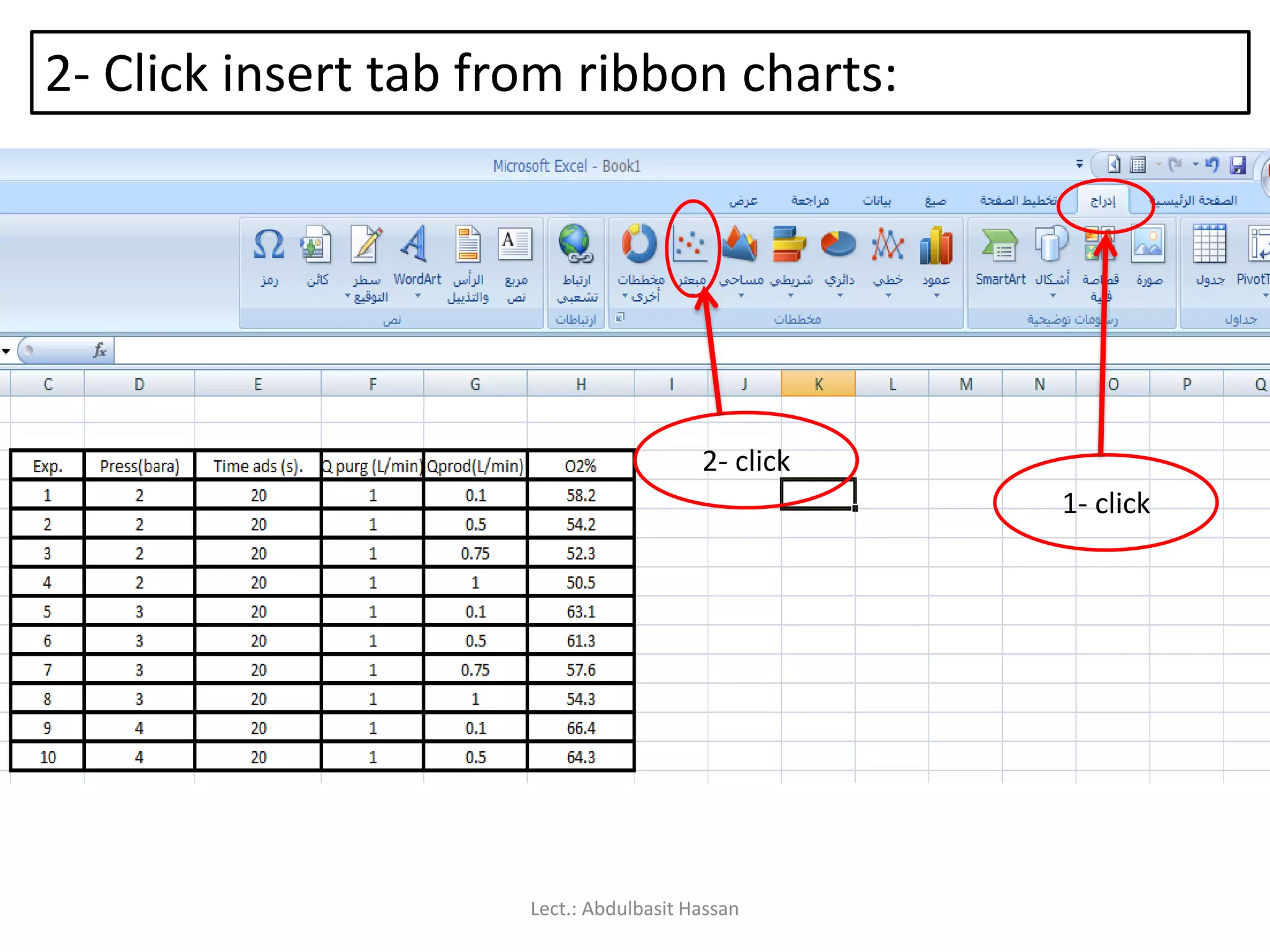
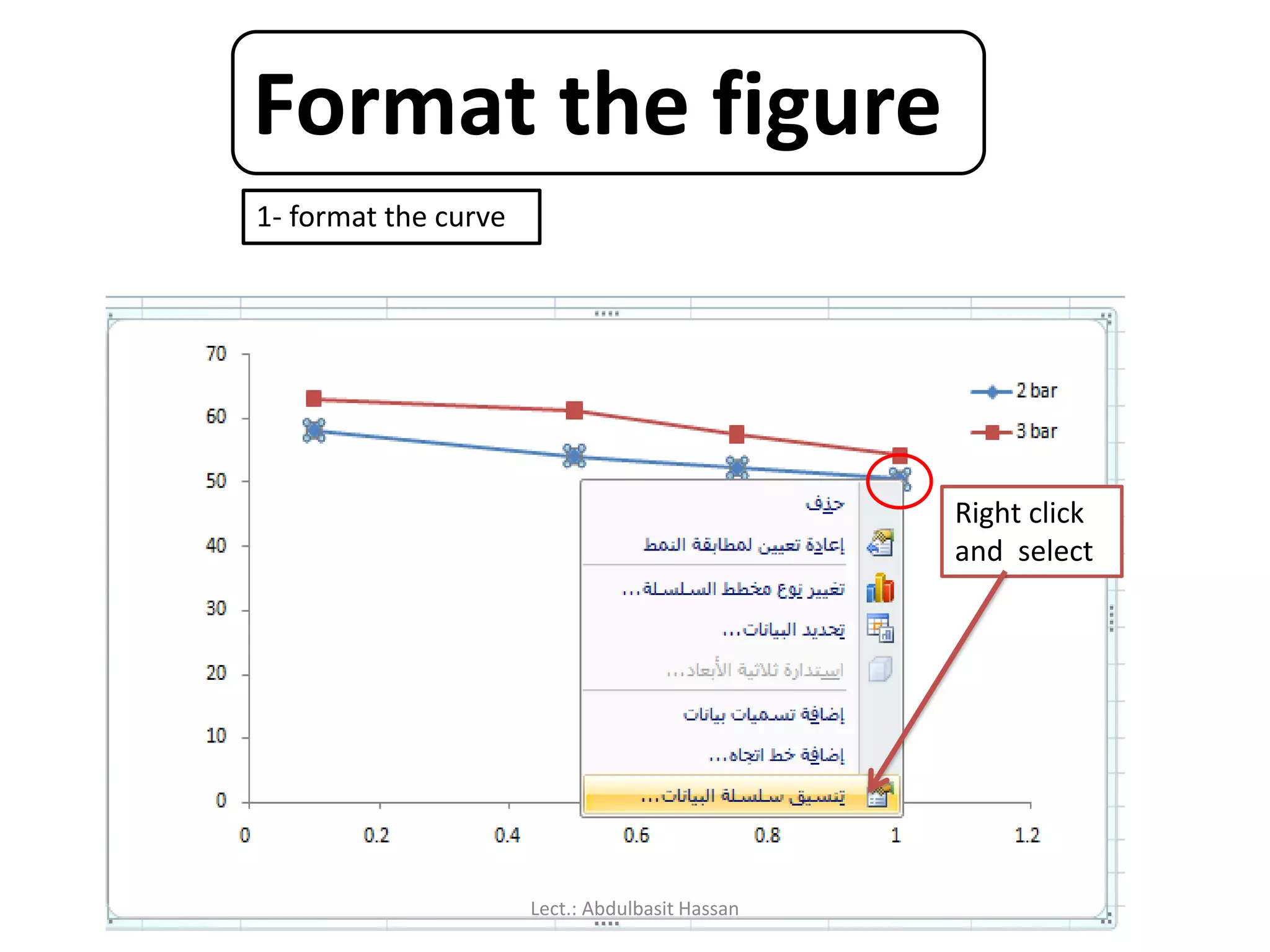
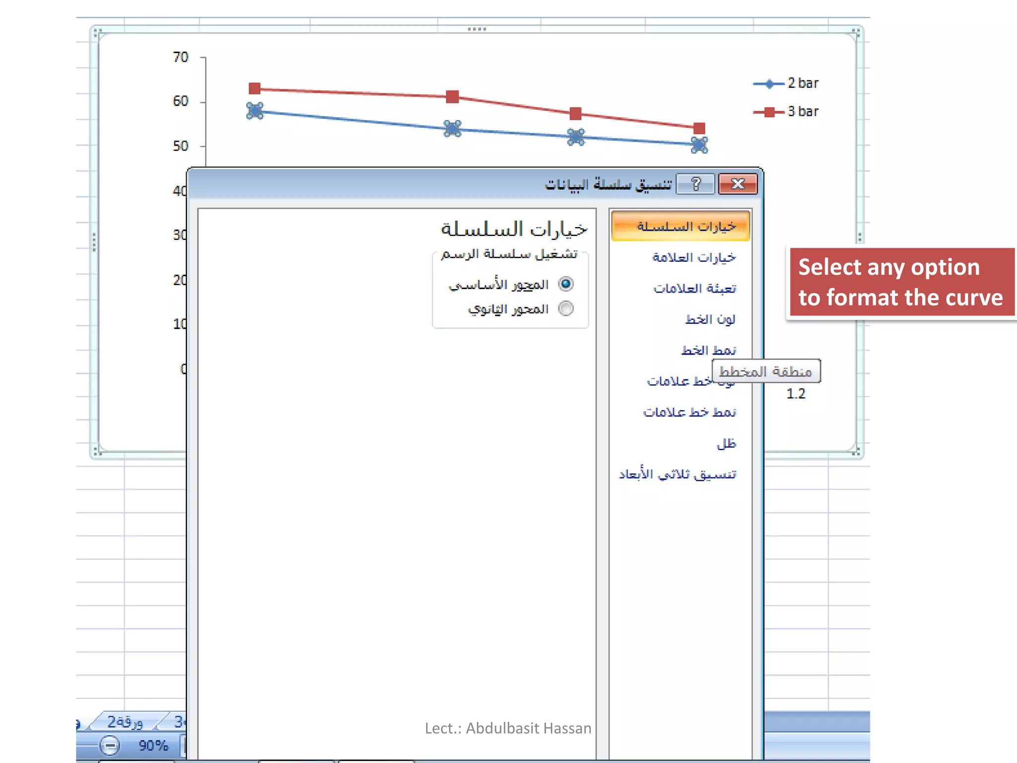
Charts allow you to present information contained in the
worksheet in a graphic format. Excel offers many types of
charts including : Column, Line, Pie, Bar, Area, Scatter and
more. To view the charts available click the Insert Tab on the
Ribbon. Lect.: Abdulbasit Hassan
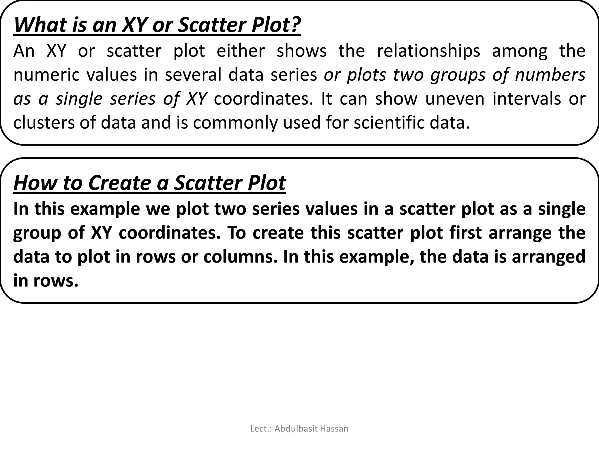
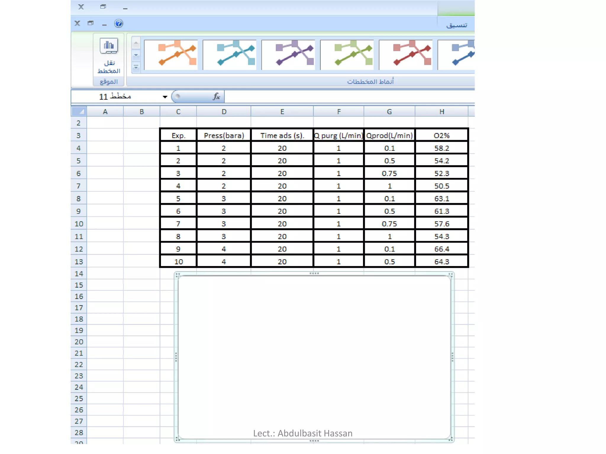
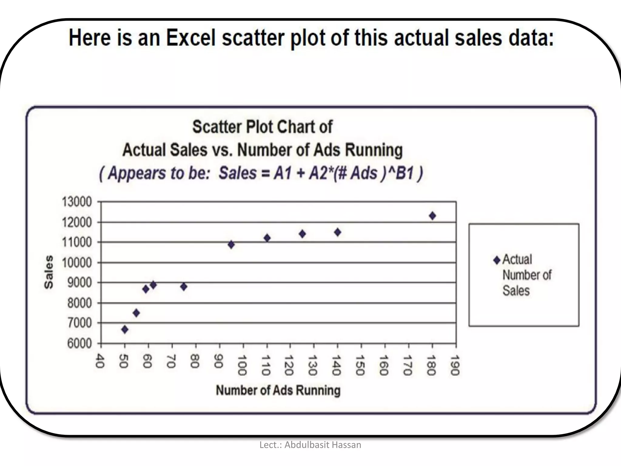
What is anXY or Scatter Plot?
An XY or scatter plot either shows the relationships among the
numeric values in several data series or plots two groups of numbers
as a single series of XY coordinates. It can show uneven intervals or
clusters of data and is commonly used for scientific data.
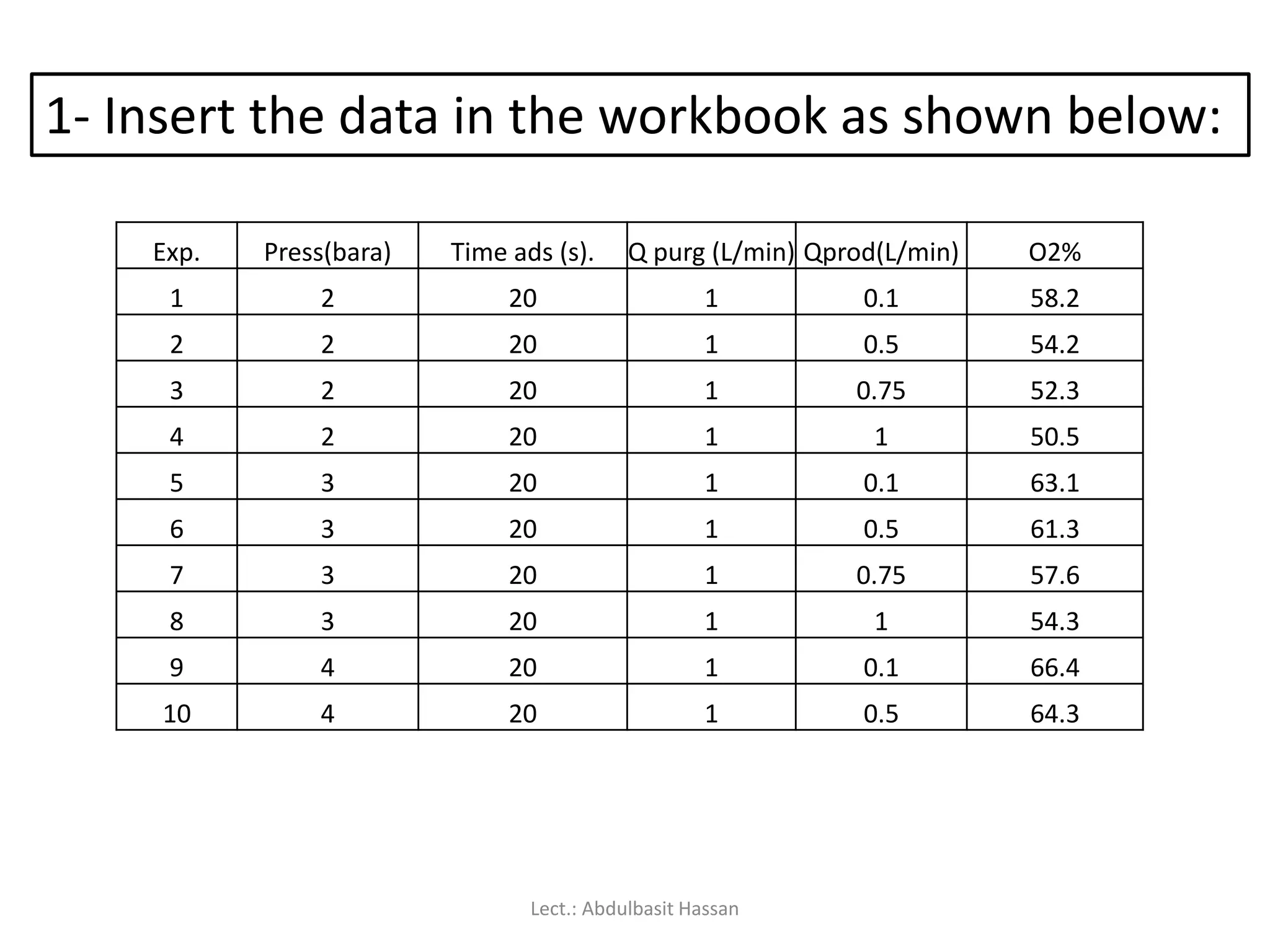
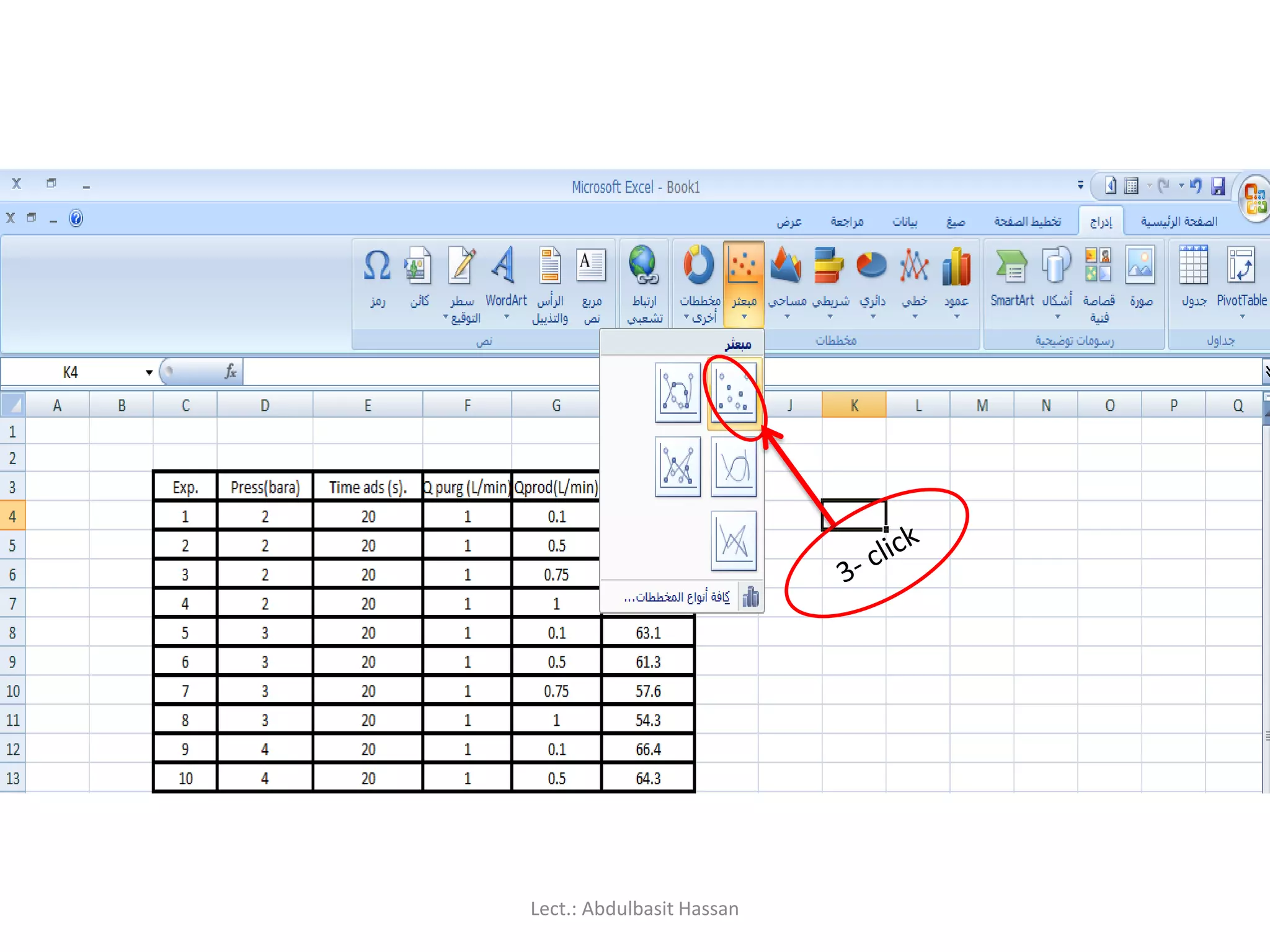
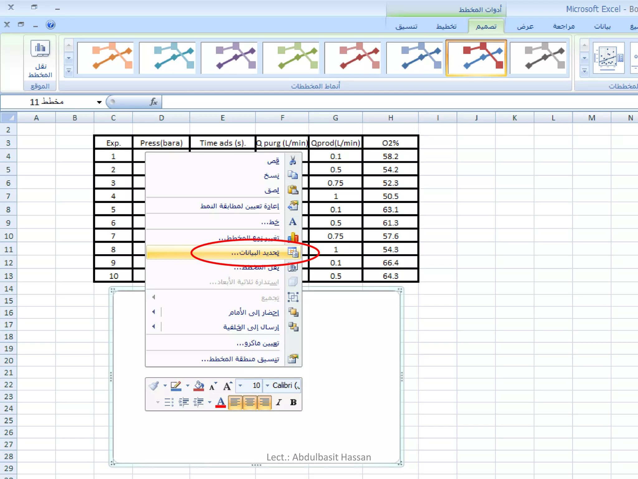
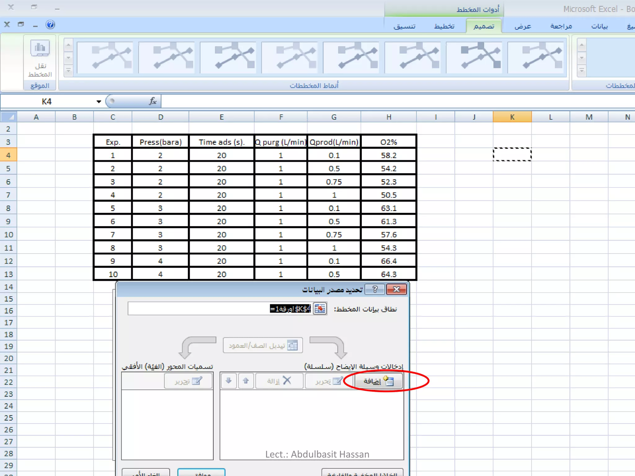
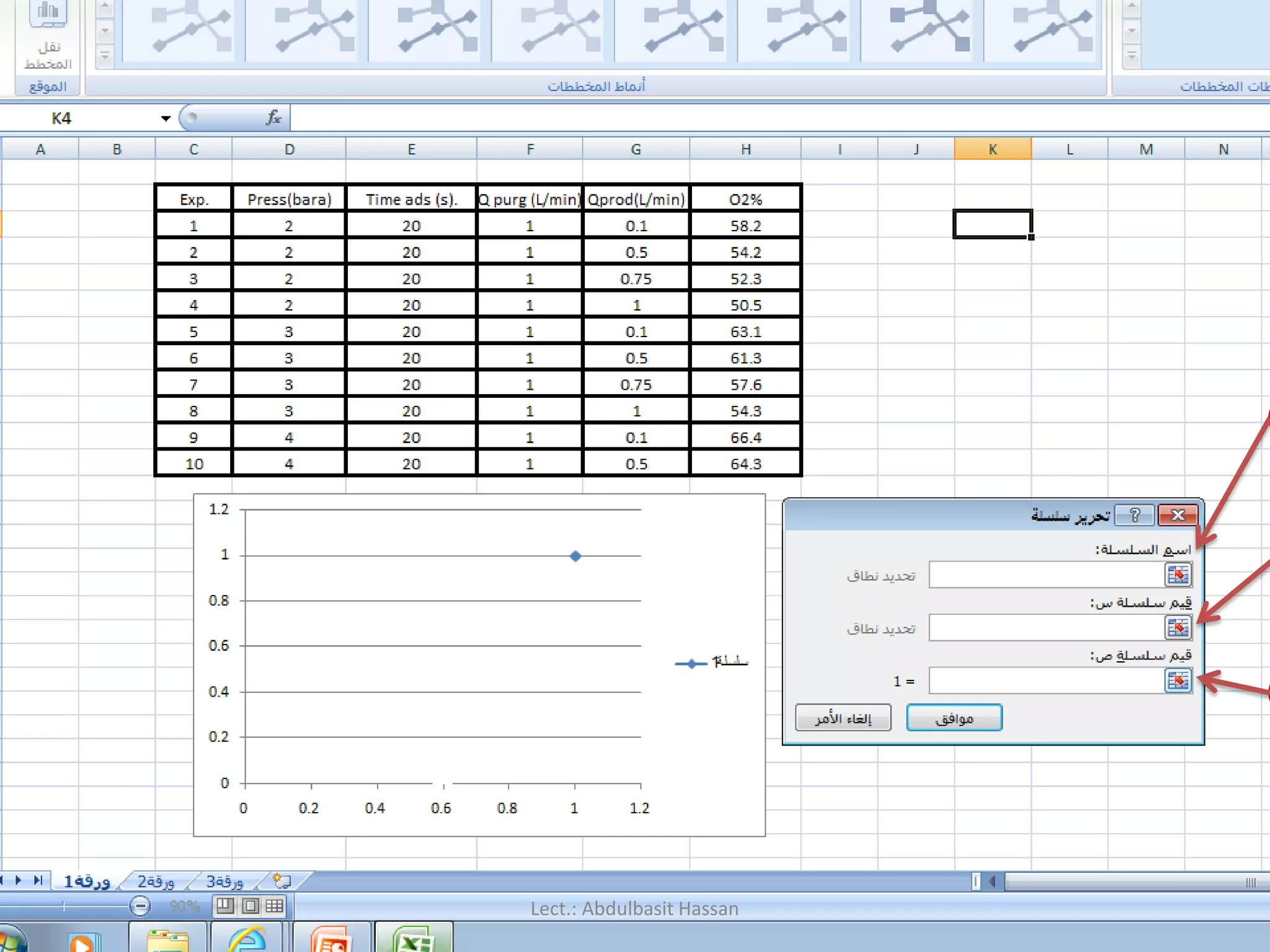
How to Create a Scatter Plot
In this example we plot two series values in a scatter plot as a single
group of XY coordinates. To create this scatter plot first arrange the
data to plot in rows or columns. In this example, the data is arranged
in rows.
Lect.: Abdulbasit Hassan
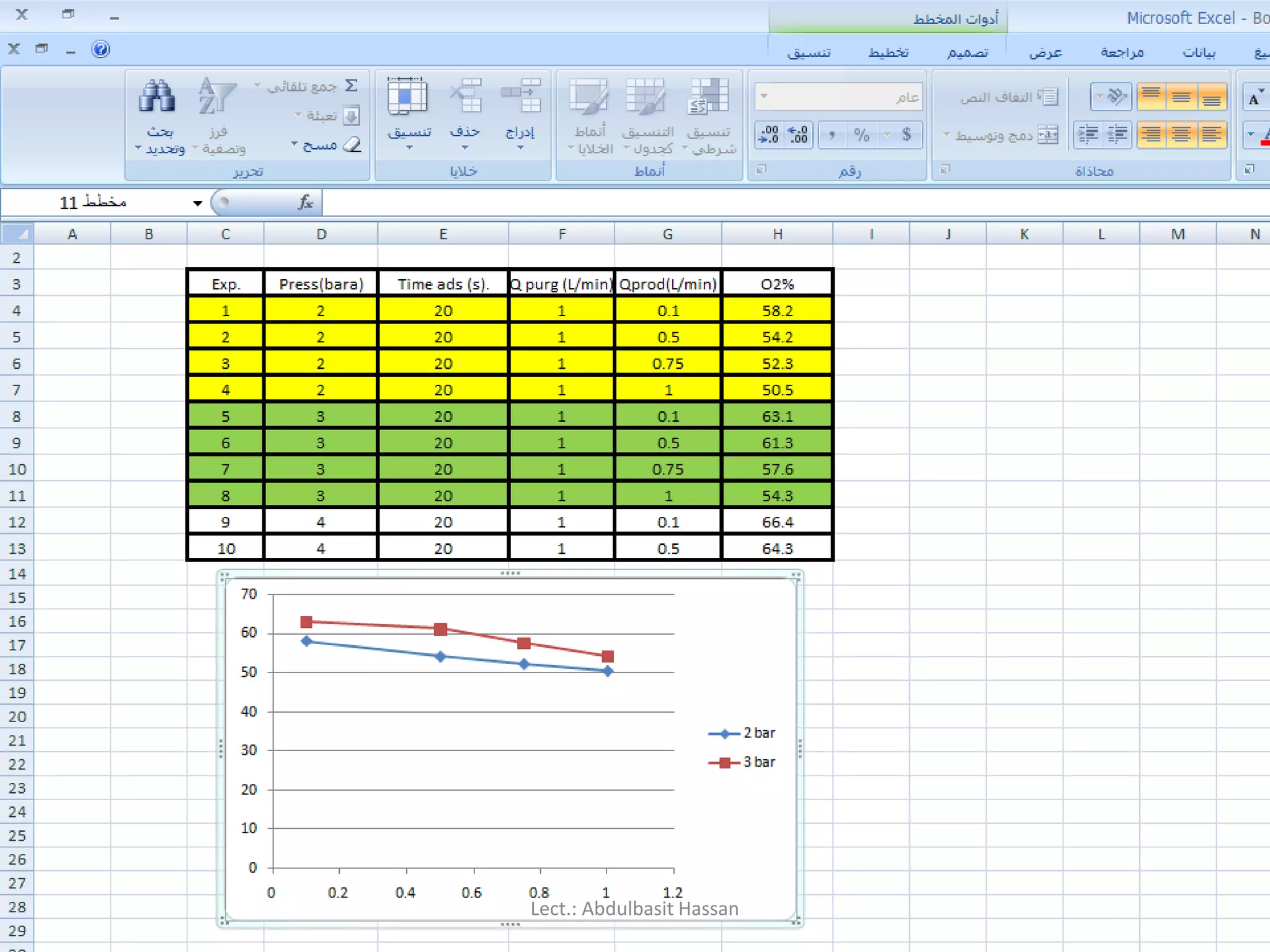
Anatomy of figure
Figure4. Isotherms of pure nitrogen on zeolite 5A.
Y-axis
Axis
label
Caption
X-axis
Symbols
Major tick
Legend
Lect.: Abdulbasit Hassan


![Using the keyboard:
Use the arrow keys, or [PAGE UP] and [PAGE DOWN], to move to
a different area of the screen.
[CTRL] + [HOME} will take you to cell A1.
[CTRL] + [PAGE DOWN] will take you to the next worksheet,
[CTRL] + [PAGE UP] for the preceding worksheet.
PAGE UP
PAGE DOWN
CTRL
arrow
HOME
You can jump quickly to a specific cell by pressing [F5] and typing
in the cell address.
You can also type the cell address in the name box above column A,
and press [ENTER].
Lect.: Abdulbasit Hassan](https://image.slidesharecdn.com/excel-200512033343/75/MS-Excel-23-2048.jpg)
![Selecting cells:
Using the mouse:
Click on a cell to select it.
You can select a range of adjacent cells by clicking on the first one,
and then dragging the mouse over the others.
You can select a set of non-adjacent cells by clicking on the first one,
and then holding down the [CTRL] key as you click on the others.
Lect.: Abdulbasit Hassan](https://image.slidesharecdn.com/excel-200512033343/75/MS-Excel-24-2048.jpg)
![Using the keyboard:
Use the arrow keys to move to the desired cell, which is
automatically selected.
To select multiple cells, hold down the [SHIFT] key while the
first cell is active, and then use the arrow keys to select the
rest of the range.
Lect.: Abdulbasit Hassan](https://image.slidesharecdn.com/excel-200512033343/75/MS-Excel-25-2048.jpg)
![Selecting rows or columns:
To select all the cells in a particular row, just click on the row
number (1, 2, 3, etc) at the left edge of the worksheet.
Hold down the mouse button and drag across row numbers to
select multiple adjacent rows.
Hold down [CTRL] if you want to select a set of non-adjacent rows.
Lect.: Abdulbasit Hassan](https://image.slidesharecdn.com/excel-200512033343/75/MS-Excel-26-2048.jpg)
![ Similarly, to select all the cells in column, you should click on the
column heading (A, B, C, etc) at the top edge of the worksheet.
Hold down the mouse button and drag across column headings to
select multiple adjacent columns.
Hold down [CTRL] if you want to select a set of non-adjacent columns.
Lect.: Abdulbasit Hassan](https://image.slidesharecdn.com/excel-200512033343/75/MS-Excel-27-2048.jpg)

![Data entry cell by cell
To enter either numbers or text:
1. Click on the cell where you want the data to be stored, so that the
cell becomes active.
2. Type the number or text.
3. Press [ENTER] to move to the next row, or [TAB] to move to the next
column. Until
4- you’ve pressed [ENTER] or [TAB], you can cancel the data entry by
pressing [ESC].
5- To enter a date, use a slash or hyphen between the day, month and
year, for example 14/02/2009. Use a colon between hours, minutes
and seconds, for example 13:45:20.
Lect.: Abdulbasit Hassan](https://image.slidesharecdn.com/excel-200512033343/75/MS-Excel-40-2048.jpg)
![Deleting data:
You want to delete data that’s already been entered in a
worksheet? Simple!
1. Select the cell or cells containing data to be deleted.
2. Press the [DEL] key on your keyboard.
3. The cells remain in the same position as before, but their
contents are deleted.
Lect.: Abdulbasit Hassan](https://image.slidesharecdn.com/excel-200512033343/75/MS-Excel-41-2048.jpg)
![Moving data :
You’ve already entered some data, and want to move it to a different
area on the worksheet?
1. Select the cells you want to move (they will become highlighted).
2. Move the cursor to the border of the highlighted cells. When the
cursor changes from a white cross to a four-headed arrow (the move
pointer), hold down the left mouse button.
3. Drag the selected cells to a new area of the worksheet, then release
the mouse button.
4. You can also cut the selected data using the ribbon icon or [CTRL] +
[X], then click in the top left cell of the destination area and paste the
data with the ribbon icon or [CTRL] + [V].
Lect.: Abdulbasit Hassan](https://image.slidesharecdn.com/excel-200512033343/75/MS-Excel-42-2048.jpg)

![Copying data:
To copy existing cell contents to another area on the worksheet:
1. Select the cells you want to copy (they will become highlighted).
2. Move the cursor to the border of the highlighted cells while hold in
down the [CTRL] key. When the cursor changes from a white cross to
a hollow left-pointing arrow (the copy pointer), hold down the left
mouse button.
3. Drag the selected cells to a second area of the worksheet, then
release the mouse button.
4. You can also copy the selected data using the ribbon icon or [CTRL] +
[C], then click in the top left cell of the destination area and paste the
data with the ribbon icon or [CTRL] + [V].
5. You can also copy the selected data by right click mouse , select copy
, and go to new cell also right click and select paste.
Lect.: Abdulbasit Hassan](https://image.slidesharecdn.com/excel-200512033343/75/MS-Excel-45-2048.jpg)

![Editing cell contents
There are two different ways to enter edit mode: either double-click on
the cell whose contents you want to edit, or else click to select the cell
you want to edit, and then click anywhere in the formula bar.
To delete characters, use the [BACKSPACE] or [DEL] key.
To insert characters, click where you want to insert them, and then
type.
You can force a line break within the current cell contents by typing
[ALT] + [ENTER], or by Space key.
Exit edit mode by pressing [ENTER].
Lect.: Abdulbasit Hassan](https://image.slidesharecdn.com/excel-200512033343/75/MS-Excel-55-2048.jpg)


![Renaming a worksheet:
Right-click on the
worksheet tab, and select
Rename from the pop-up
menu. Type the new
worksheet name and press
[ENTER].
Lect.: Abdulbasit Hassan](https://image.slidesharecdn.com/excel-200512033343/75/MS-Excel-71-2048.jpg)

![Using AutoSum:
Because addition is the most frequently used Excel function, a shortcut
has been provided to quickly add a set of numbers:
1. Select the cell where you want the total to appear.
2. Click on the Sum button on the Home ribbon.
3. Check that the correct set of numbers has been selected (indicated by
a dotted line). If not, then drag to select a different set of numbers.
4. Press [ENTER] and the total will be calculated.
Lect.: Abdulbasit Hassan](https://image.slidesharecdn.com/excel-200512033343/75/MS-Excel-101-2048.jpg)
![Several popular functions are available to you directly from the Home
ribbon.
1. Select the cell where you want the result of the calculation to be
displayed.
2. Click the drop-down arrow next to the Sum button.
3. Click on the function that you want.
4. Confirm the range of cells that the function should use in its
calculation.
5. Press [ENTER]. The result of the calculation will be shown in the active
cell.
Lect.: Abdulbasit Hassan](https://image.slidesharecdn.com/excel-200512033343/75/MS-Excel-106-2048.jpg)
![As an example, to calculate the average for the following set of tutorial
results, you would:
1. Click on cell F3 to make it active.
2. Click on the arrow next to the Sum button, and select Average.
3. Press [ENTER] to accept the range of cells that is suggested (B3:E3).
That’s it! You can now copy the formula in cell F3 down to cells F4 and
F5 – using relative addressing because you want a different set of
tutorial marks to be used for each student.
Lect.: Abdulbasit Hassan](https://image.slidesharecdn.com/excel-200512033343/75/MS-Excel-107-2048.jpg)


![The task now is to determine the best values for k1 and k2. However,
the expression of [B] is non-linear, and not easily transformed into a
linear form. We can, however, use “Solver” to accomplish the same
task.
Lect.: Abdulbasit Hassan](https://image.slidesharecdn.com/excel-200512033343/75/MS-Excel-159-2048.jpg)
![To start we need to make initial estimates for both k1 and k2. Let’s
use 1 and 2. (Note: We don’t want to use the same value for both k1
and k2 since that would make the denominator term in the
expression for [B] zero.) With these two values we can use the
expression for [B] to calculate values for the concentration of B.
Lect.: Abdulbasit Hassan](https://image.slidesharecdn.com/excel-200512033343/75/MS-Excel-160-2048.jpg)
![3- [X] = [A] * [b]-1
Lect.: Abdulbasit Hassan](https://image.slidesharecdn.com/excel-200512033343/75/MS-Excel-165-2048.jpg)