Molecular Dynamics Computer Experiment (Hebrew)

‫ניס‬‫ו‬‫מחשב‬ ‫י‬‫בדינאמיק‬‫ה‬‫מולקולארי‬‫ת‬
‫מדריך‬:‫שרוני‬ ‫ינון‬,‫ד‬‫וא‬"‫ל‬:inonshar@tau.ac.il
‫עמוד‬‫ה‬‫אינטרנט‬‫הניסוי‬ ‫של‬:http://www.tau.ac.il/~physchem/Dynamics/index.htm
‫הניסוי‬ ‫בבניית‬ ‫השתתפו‬:
‫פרופ‬'‫ניצן‬ ‫אברהם‬1002-
‫דר‬'‫שק‬ ‫ישראל‬1002-
‫כלב‬ ‫יואל‬1002-1002
‫דר‬'‫יעקבי‬ ‫חני‬1002-1002
‫דר‬'‫מרוז‬ ‫יסמין‬1002-1022
‫קכמן‬ ‫טל‬1021
‫שרוני‬ ‫ינון‬1022

‫מולקולארית‬ ‫בדינאמיקה‬ ‫מחשב‬ ‫ניסוי‬‫מדריך‬:Inon Sharony
‫מבוא‬1
‫מבוא‬
‫הקדמה‬
‫ז‬ ‫ניסוי‬ ‫מטרת‬‫להעניק‬ ‫ה‬,‫בכ‬ ‫המעוניין‬ ‫לתלמיד‬‫ך‬,‫ב‬ ‫ראשונה‬ ‫התנסות‬‫עבודתו‬‫כתיאורטיק‬‫ן‬‫חישובי‬.‫הניסוי‬
‫בקורסים‬ ‫יותר‬ ‫מלא‬ ‫באופן‬ ‫שנלמדים‬ ‫ידע‬ ‫תחומי‬ ‫במספר‬ ‫נוגע‬‫תיאורטיי‬‫ם‬‫כגון‬:‫נומריות‬ ‫שיטות‬,‫מעבדה‬
‫חישובית‬ ‫בכימיה‬,‫תרמודינאמיקה‬‫אקראיים‬ ‫ומהלכים‬ ‫סטטיסטית‬.‫הנ‬ ‫מהקורסים‬ ‫אחד‬ ‫אף‬"‫מהווה‬ ‫לא‬ ‫ל‬
‫דרי‬‫הניסוי‬ ‫לביצוע‬ ‫קדם‬ ‫שת‬.‫חישובית‬ ‫מעבודה‬ ‫נמנע‬ ‫בלתי‬ ‫חלק‬ ‫הינו‬ ‫התכנות‬,‫שמדען‬ ‫לומר‬ ‫בכך‬ ‫אין‬ ‫אך‬
‫מתכנת‬ ‫במהותו‬ ‫הוא‬ ‫חישובי‬.‫תכנות‬ ‫עבודת‬ ‫התלמידים‬ ‫יבצעו‬ ‫הניסוי‬ ‫במסגרת‬‫מסוימת‬,‫כן‬ ‫שאלמלא‬
‫אמינה‬ ‫הייתה‬ ‫לא‬ ‫החוויה‬.‫זאת‬ ‫עם‬,‫הדגש‬‫הינו‬‫על‬ ‫ההסתכלות‬‫תכנות‬‫לא‬‫ככלי‬ ‫אלא‬ ‫כמטרה‬.
‫סימולציו‬‫מחשב‬ ‫ת‬
‫מופשט‬ ‫מתמטי‬ ‫מודל‬ ‫להדמיית‬ ‫שמשמת‬ ‫מחשב‬ ‫תוכנת‬ ‫היא‬ ‫מחשב‬ ‫סימולציית‬,‫דגם‬ ‫או‬,‫נתונה‬ ‫מערכת‬ ‫של‬.
‫מתחיי‬ ‫לעיתים‬ ‫מחשב‬ ‫באמצעות‬ ‫פתרון‬‫ב‬‫אנאליטי‬ ‫פתרון‬ ‫אין‬ ‫המתמטי‬ ‫שלמודל‬ ‫מוכח‬ ‫כאשר‬,‫פתרון‬ ‫אם‬
‫אינו‬ ‫פשוט‬ ‫שכזה‬‫ישים‬.‫כלומר‬,‫אנאליטי‬ ‫פתרון‬ ‫למציאת‬ ‫הנדרשים‬ ‫המשאבים‬ ‫אם‬,‫פתר‬ ‫לעומת‬‫נומרי‬ ‫ון‬,‫הם‬
‫להשקיע‬ ‫ברצוננו‬ ‫מאשר‬ ‫רבים‬.‫נוכל‬ ‫שבהצבתם‬ ‫ופרמטרים‬ ‫משתנים‬ ‫של‬ ‫כפונקציה‬ ‫ייראה‬ ‫אנאליטי‬ ‫פתרון‬
‫מספרי‬ ‫פתרון‬ ‫לקבל‬(‫נומרי‬.)‫כללי‬ ‫אנליטי‬ ‫פתרון‬ ‫בידנו‬ ‫אין‬ ‫אם‬,‫מקומיות‬ ‫קירוב‬ ‫בשיטות‬ ‫להשתמש‬ ‫נוכל‬
‫איטרטיבי‬ ‫פתרון‬ ‫לבנות‬ ‫בכדי‬,‫מחשב‬ ‫באמצעות‬ ‫למימוש‬ ‫המותאם‬.‫סימולציות‬‫ורק‬ ‫אך‬ ‫מטפלות‬ ‫נומריות‬
‫מופשטת‬ ‫באלגברה‬ ‫ולא‬ ‫המעורבים‬ ‫המשתנים‬ ‫של‬ ‫המספריים‬ ‫בערכים‬(‫שכיום‬ ‫למרות‬‫קיימות‬‫תכניות‬
‫זה‬ ‫את‬ ‫אפילו‬ ‫לעשות‬ ‫שיודעות‬ ‫מחשב‬.)
‫מתמטי‬ ‫מידול‬
‫בבניית‬‫הדגם‬,‫הפשטה‬ ‫הינו‬ ‫המפתח‬.‫א‬ ‫ועד‬ ‫אריסטו‬ ‫מאז‬ ‫שאמרו‬ ‫כפי‬‫י‬‫ינשטיין‬" :‫הכו‬‫ל‬‫צריך‬‫להיעשו‬‫ת‬‫בצורה‬
‫ביותר‬ ‫הפשוטה‬,‫א‬‫מכך‬ ‫פשוט‬ ‫לא‬ ‫ך‬".‫בהקשרים‬‫מסוימים‬,‫אוקאם‬ ‫של‬ ‫תערו‬ ‫זו‬ ‫מימרה‬ ‫המכנים‬ ‫יש‬.
‫מורכבות‬ ‫של‬ ‫שונות‬ ‫רמות‬ ‫לכלול‬ ‫יכולות‬ ‫מחשב‬ ‫סימולציות‬,‫וגדלות‬ ‫הולכות‬ ‫משאבים‬ ‫רמות‬ ‫ולדרוש‬
‫בהתאם‬,‫ועד‬ ‫ידנית‬ ‫מאיטרציה‬ ‫החל‬‫למחשוב‬-‫מבוזר‬ ‫על‬.‫נקראים‬ ‫לעיתים‬ ‫במחשב‬ ‫המבוצעים‬ ‫ניסיונות‬
‫בהתלוצצות‬"in silico."
‫נומרי‬ ‫פתרון‬
‫שונים‬ ‫מתמטיים‬ ‫ניסוחים‬ ‫באמצעות‬ ‫בעיות‬ ‫למדל‬ ‫ניתן‬,‫עצמיים‬ ‫וערכים‬ ‫אפסים‬ ‫מציאת‬ ‫למשל‬ ‫הכוללים‬,
‫ואינטגרציה‬ ‫גזירה‬,‫וסטטיסטיקה‬ ‫הסתברות‬,‫ואופטימיזציה‬ ‫קומבינטוריקה‬(‫לדוגמה‬,‫וריאציות‬ ‫חשבון‬)
‫ועוד‬.‫הפתרון‬ ‫למציאת‬ ‫נומריות‬ ‫שיטות‬ ‫מספר‬ ‫להתאים‬ ‫יכולות‬ ‫ניסוח‬ ‫לכל‬.
‫בנוסף‬,‫הנ‬ ‫החישובים‬ ‫את‬ ‫מאד‬ ‫המייעלים‬ ‫אלגוריתמים‬ ‫פותחו‬"‫ל‬,‫נתונים‬ ‫במבני‬ ‫וחיפוש‬ ‫מיון‬ ‫עבור‬ ‫לדוגמה‬.
‫מחשב‬ ‫באמצעות‬ ‫פתרון‬ ‫של‬ ‫יתרונות‬
‫יתרונות‬ ‫כמה‬ ‫איתו‬ ‫נושא‬ ‫בעיות‬ ‫לפתרון‬ ‫במחשב‬ ‫שימוש‬.‫לדוגמה‬,‫אינדוקטיבית‬ ‫חשיבה‬ ‫מאפשר‬ ‫הוא‬
(‫אינטואיציה‬ ‫הסקת‬‫ותיאורי‬‫ה‬‫של‬ ‫סופית‬ ‫מקבוצה‬ ‫כללית‬‫פרטיים‬ ‫מקרים‬.)‫בנוסף‬,‫בהם‬ ‫מקרים‬ ‫ישנם‬
‫פתרון‬ ‫את‬ ‫מייעלת‬ ‫מחשב‬ ‫ידי‬ ‫על‬ ‫המיוצרת‬ ‫אקראיות‬‫הבעיה‬,‫אם‬ ‫גם‬‫הבעיה‬‫דטרמיניסטית‬ ‫לחלוטין‬(‫כלומר‬
‫אקראית‬ ‫לא‬.)‫דוגמ‬‫ה‬‫אינטגרצי‬ ‫היא‬ ‫מפורסמת‬‫שם‬ ‫על‬ ‫האלגוריתמים‬ ‫משפחת‬ ‫באמצעות‬ ‫ה‬‫ההימורים‬ ‫ערי‬
‫קרלו‬ ‫מונטה‬‫ווגאס‬ ‫ולאס‬.‫שימ‬ ‫שעושים‬ ‫אלגוריתמים‬‫סטוכסטיים‬ ‫אלגוריתמים‬ ‫נקראים‬ ‫באקראיות‬ ‫וש‬.
"‫חסרי‬ ‫הם‬ ‫מחשבים‬‫תועלת‬.‫תשובות‬ ‫רק‬ ‫לתת‬ ‫יודעים‬ ‫הם‬".–‫פיקאסו‬ ‫פבלו‬,2291
‫לפרשן‬ ‫ובדרכים‬ ‫אלו‬ ‫תשובות‬ ‫השגת‬ ‫באופן‬ ‫נתמקד‬ ‫במעבדה‬.

‫מבוא‬2
‫דינאמיקה‬‫מולקולארית‬
‫מולקולארית‬ ‫דינאמיקה‬(Molecular Dynamics, MD)‫תכו‬ ‫של‬ ‫שיערוך‬ ‫המאפשרת‬ ‫שיטה‬ ‫היא‬‫נות‬‫מקרוסקופיות‬
(‫תרמודינאמיות‬ ‫תכונות‬ ‫כגון‬)‫באמצעות‬‫מיקרוסקופיים‬ ‫תהליכים‬ ‫הדמיית‬‫גבי‬ ‫על‬ ‫ומיצוע‬‫של‬ ‫צברים‬
‫חלקיקי‬‫ם‬.‫ניוטון‬ ‫של‬ ‫התנועה‬ ‫משוואות‬ ‫של‬ ‫נומרי‬ ‫פתרון‬ ‫על‬ ‫מבוססת‬ ‫היא‬,‫ההנחה‬ ‫תחת‬‫שהמכאניק‬‫ה‬
‫קבילה‬ ‫הקלאסית‬.
‫מדוע‬‫מכאניק‬‫ה‬‫קלאסית‬?
‫השאלה‬ ‫עולה‬:"‫להשתמש‬ ‫מדוע‬‫במכאניק‬‫ה‬‫מסתמן‬ ‫כאשר‬ ‫הקלאסית‬‫שזו‬‫הקוונטית‬‫ביקום‬ ‫המושלת‬ ‫היא‬?"
‫לשימוש‬ ‫המניע‬‫במכאניק‬‫ה‬‫ה‬ ‫הקלאסית‬‫ו‬‫מחשוב‬ ‫משאבי‬ ‫בצריכת‬ ‫המעריכית‬ ‫העלייה‬ ‫א‬(‫וזיכרון‬ ‫מעבד‬ ‫זמן‬)
‫לפתרון‬‫קוונטי‬,‫החישוב‬ ‫את‬ ‫עושים‬ ‫שעבורה‬ ‫המערכת‬ ‫שגדלה‬ ‫ככל‬.‫אולם‬,‫מערכות‬ ‫שעבור‬ ‫להראות‬ ‫ניתן‬
‫סבירים‬ ‫טמפרטורות‬ ‫בטווחי‬ ‫רבות‬,‫המכאניק‬‫ה‬‫טוב‬ ‫קירוב‬ ‫מהווה‬ ‫הקלאסית‬.
‫משטח‬ ‫בחירת‬‫הפוטנציאל‬
‫הבין‬ ‫האינטראקציות‬-‫והבין‬ ‫אטומיות‬-‫מולקולאריו‬‫ת‬,‫המערכת‬ ‫של‬ ‫הפוטנציאלית‬ ‫האנרגיה‬ ‫מכך‬ ‫וכתוצאה‬,
‫באמצעות‬ ‫לתיאור‬ ‫ניתנות‬‫של‬ ‫רב‬ ‫מגוון‬‫פונקציו‬‫ת‬.‫התכונות‬ ‫את‬ ‫לשקף‬ ‫צריכה‬ ‫הפוטנציאל‬ ‫משטח‬ ‫בחירת‬
‫הנדו‬ ‫המערכה‬ ‫של‬ ‫הפיזיקאליות‬‫נה‬.‫גבוהה‬ ‫בשכיחות‬ ‫הנמצאות‬ ‫תכונות‬‫בדגמים‬‫הן‬ ‫קיימים‬,‫לדוגמה‬,
‫זמן‬ ‫ובאותו‬ ‫במרחב‬ ‫נקודה‬ ‫באותה‬ ‫להימצא‬ ‫יוכלו‬ ‫לא‬ ‫אטומים‬ ‫ששני‬ ‫הדרישה‬(‫קולומבית‬ ‫דחייה‬ ‫לדמות‬ ‫בכדי‬
‫פאולי‬ ‫דחיית‬ ‫או‬)‫גדולים‬ ‫במרחקים‬ ‫תדעך‬ ‫ושהאינטראקציה‬.
‫הפרמטרים‬ ‫כיול‬
‫באמצע‬ ‫הפוטנציאל‬ ‫של‬ ‫הפרמטרים‬ ‫את‬ ‫לכייל‬ ‫נהוג‬‫בניסיון‬ ‫שהושג‬ ‫במידע‬ ‫שימוש‬ ‫ות‬.‫את‬ ‫הופכת‬ ‫זו‬ ‫עובדה‬
‫לסמי‬ ‫החישוב‬-‫מטבעו‬ ‫אמפירי‬.

‫מבוא‬1
‫ה‬‫מקור‬‫ל‬ ‫ההיסטורי‬‫ניסוי‬
‫ראהמאן‬ ‫אניסור‬ ‫ידי‬ ‫על‬ ‫במקור‬ ‫בוצע‬ ‫הניסוי‬,‫הדינאמיקה‬ ‫ואבי‬ ‫החישובית‬ ‫הפיזיקה‬ ‫מחלוצי‬‫המולקולארית‬.
‫במ‬‫שלו‬ ‫המייסד‬ ‫אמר‬‫משנת‬2291,‫ביצע‬‫סימולציה‬‫של‬291‫ארגון‬ ‫אטומי‬,‫לנרד‬ ‫אינטראקציות‬ ‫עם‬-‫ג‬'‫ונס‬,
‫הנוזלי‬ ‫במצב‬ ‫ארגון‬ ‫לדימוי‬.‫מסוג‬ ‫מחשב‬ ‫על‬ ‫נערך‬ ‫הניסוי‬CDC 3600.
‫מותו‬ ‫לאחר‬,‫קראה‬ ‫לפיזיקה‬ ‫האמריקאית‬ ‫שהחברה‬ ‫בכך‬ ‫ראהמאן‬ ‫כובד‬‫על‬ ‫חישובית‬ ‫בפיזיקה‬ ‫שלה‬ ‫לפרס‬
‫שמו‬‫קראה‬ ‫בארגון‬ ‫הלאומית‬ ‫שהמעבדה‬ ‫ובכך‬‫פוסט‬ ‫מלגות‬ ‫לתכנית‬-‫דוקטורט‬‫שמו‬ ‫על‬.
‫מה‬‫ת‬‫במעבדה‬ ‫עשה‬
‫בדינאמיקה‬ ‫במעבדה‬ ‫ניסיונך‬ ‫במהלך‬‫מולקולארי‬‫ת‬,‫פי‬ ‫בעיות‬ ‫לנתח‬ ‫תלמד‬‫של‬ ‫עיניו‬ ‫מבעד‬ ‫זיקאליות‬
‫תיאורטיק‬‫ן‬‫חישובי‬.‫חלקים‬ ‫משלושה‬ ‫מורכב‬ ‫הניסיון‬,‫בהם‬
‫א‬.‫ת‬‫כת‬‫ו‬‫המגרילה‬ ‫תכנית‬ ‫ב‬‫אקראיים‬ ‫מספרים‬‫תכונותיהם‬ ‫את‬ ‫ומנתחת‬‫שצברת‬ ‫בידע‬ ‫ותשתמש‬
‫המיקרוסקופית‬ ‫ברמה‬ ‫דיפוזיה‬ ‫תהליך‬ ‫לדמות‬.
‫ב‬.‫במחשב‬ ‫תשתמש‬‫משוואות‬ ‫את‬ ‫נומרית‬ ‫לפתור‬ ‫כדי‬‫של‬ ‫התנועה‬‫ניוטון‬‫אוסילטור‬ ‫עבור‬‫הרמוני‬,
‫ול‬‫מצות‬‫תכונות‬‫תרמו‬‫דינמיות‬‫מ‬ ‫המערכת‬ ‫של‬‫התוצאות‬‫המתקבלות‬.
‫ג‬.‫של‬ ‫והתרמודינמיות‬ ‫המבניות‬ ‫התכונות‬ ‫את‬ ‫תנתח‬‫ארגון‬‫הנוזלי‬ ‫במצב‬,‫שתפיק‬ ‫נתונים‬ ‫באמצעות‬
‫מסימולציית‬‫דינאמיק‬‫ה‬‫מולקולארי‬‫ת‬.
‫ממך‬ ‫מצופה‬ ‫מה‬
‫א‬.‫מוכן‬ ‫הגע‬--‫הקלעים‬ ‫שמאחרי‬ ‫והנומריקה‬ ‫הפיזיקה‬ ‫את‬ ‫הבן‬.
‫ב‬.‫ס‬ ‫היה‬‫בלני‬--‫מחשבך‬ ‫אל‬ ‫נחמד‬ ‫היה‬!
‫ג‬.‫יצירתי‬ ‫היה‬!
‫משקל‬‫וציון‬
‫דו‬"‫מכינים‬ ‫חות‬3 × 10% = 30%(2‫דו‬"‫מפגש‬ ‫כל‬ ‫לקראת‬ ‫שיוגשו‬ ‫נפרדים‬ ‫מכינים‬ ‫חות‬)
‫המדריך‬ ‫הערכת‬10%(‫מוכנות‬,‫קשב‬,‫יעילות‬,‫יסודיות‬,‫סקרנות‬,‫יצירתיות‬)
‫דו‬"‫מסכם‬ ‫ח‬3 × 20% = 60%(‫בדו‬ ‫פרק‬ ‫לכל‬ ‫נפרד‬ ‫ציון‬"‫פ‬ ‫לפי‬ ‫המסכם‬ ‫ח‬‫הניסוי‬ ‫רקי‬)
‫הסופי‬ ‫לציון‬ ‫הישר‬ ‫משוקללות‬ ‫בונוס‬ ‫נקודות‬.

‫מבוא‬2
‫תוכן‬‫העניינים‬
‫מבוא‬................................................................................................................................................................1
‫הקדמה‬.........................................................................................................................................................1
‫סימולציות‬‫מחשב‬........................................................................................................................................1
‫דינאמיקה‬‫מולקולארית‬...............................................................................................................................2
‫מה‬‫תעשה‬‫במעבדה‬.....................................................................................................................................1
‫מה‬‫מצופה‬‫ממך‬...........................................................................................................................................1
‫הכנות‬‫לניסוי‬...............................................................................................................................................9
‫דרישות‬‫לדו‬"‫ח‬‫המסכם‬................................................................................................................................2
‫הערות‬‫לש‬‫יפור‬‫המעבדה‬............................................................................................................................21
‫שימוש‬‫מרוחק‬‫במשאבי‬‫המחשוב‬‫האוניברסיטאיים‬.................................................................................21
‫א‬.‫סימולציית‬‫תהליכים‬‫סטוכסטיים‬(‫מקרה‬‫בוחן‬:‫המהלך‬‫האקראי‬‫הפשוט‬)...............................................22
‫בשלב‬‫זה‬‫של‬‫הניסוי‬..................................................................................................................................22
‫חובת‬‫קריאה‬..............................................................................................................................................22
‫דו‬"‫ח‬‫מכין‬...................................................................................................................................................22
‫ביצוע‬‫הניסוי‬.............................................................................................................................................21
‫ב‬.‫סימולציית‬‫מכאניקה‬‫ניוטונית‬(‫מקרה‬‫בוחן‬:‫תנועה‬‫בפוטנציאל‬‫הרמוני‬).................................................22
‫בשלב‬‫זה‬‫של‬‫הניסוי‬..................................................................................................................................22
‫חובת‬‫קריאה‬..............................................................................................................................................22
‫דו‬"‫ח‬‫מכין‬...................................................................................................................................................19
‫ביצוע‬‫הניסוי‬.............................................................................................................................................12
‫ג‬.‫סימולציית‬‫דינאמיקה‬‫מולקולארית‬(‫מקרה‬‫בוחן‬:‫שיווי‬‫משקל‬‫של‬‫ארגון‬‫נוזלי‬).......................................22
‫בשלב‬‫זה‬‫של‬‫הניסוי‬..................................................................................................................................22
‫חובת‬‫קריאה‬..............................................................................................................................................22
‫דו‬"‫ח‬‫מכין‬...................................................................................................................................................99
‫ביצוע‬‫הניסוי‬.............................................................................................................................................92

‫מבוא‬9
‫לניסוי‬ ‫הכנות‬
‫ספר‬‫לשאול‬ ‫שיש‬ ‫ים‬
‫עיקריים‬ ‫מקורות‬(‫חובה‬)
‫א‬.‫תיאורט‬ ‫רקע‬‫י‬:
 Abraham Nitzan, Chemical Dynamics in Condensed Phases, Oxford University
Press (2006).
‫ב‬.‫שיטת‬‫הדינאמיקה‬‫המולקולארית‬:
 Daan Frenkel & Berend Smit, Understanding Molecular Simulations, Second Edition, Academic
Press (2002).
‫נוספים‬ ‫מקורות‬
‫ג‬.‫ניוטון‬ ‫משוואות‬ ‫של‬ ‫נומרי‬ ‫פתרון‬:
 Gould & Tobochnik, An Introduction to Computer Simulation Methods, third edition, Pearson
(2007).
‫ד‬.‫סימולצי‬‫ו‬‫ת‬‫נוזלים‬ ‫של‬:
 A.Rahman, "Correlations in the Motion of Atoms in Liquid Argon," Phys. Rev. A 136 P. A405, 1964.
 L. Verlet, "Computer Experiments on Classical Fluids. I. Thermodynamical Properties of Lennard-
Jones Molecules," Phys. Rev. 159, 98 (1967).
 D. W. Heermann, Computer Simulation Methods in Theoretical Physics, second edition, Springer
(1990).
 M.P. Allen & D.J. Tildesley, Computer Simulation of Liquids, Oxford University Press (1991). A 2003
version also exists.
‫ה‬.‫אקראיים‬ ‫מספרים‬‫בזמן‬ ‫וקורלציה‬:
 Frederick Reif, Fundamentals of Statistical and Thermal Physics, McGraw-Hill (1965). A 2008
version also exists.
‫ו‬.‫נוזלים‬ ‫של‬ ‫מרחביות‬ ‫קורלציה‬ ‫פונקציות‬:
 David Chandler, Introduction to Modern Statistical Mechanics, Oxford University Press (1987).
‫להרחבה‬ ‫קריאה‬
‫ז‬.‫נומריות‬ ‫שיטות‬:
 Steven E. Koonin & Dawn C. Meredith, Computational Physics: FORTRAN Version, Addison-Wesley
(1990).
 Richard J. Sadus, Molecular Simulation of Fluids: Theory, Algorithms and Object-Orientation,
Elsevier (2002).
 Numerical Recipes: The Art of Scientific Computing, Third Edition (C++), Cambridge University
Press (2007). Limited free access on www.nr.com (full access for second edition 1992 in C or
FORTRAN).
‫ח‬.‫נוזלים‬ ‫של‬ ‫תכונות‬:
 Jean-Pierre Hansen & I.R. McDonald, Theory of Simple Liquids, 3
rd
edition, Academic Press (2006).

‫מבוא‬2
‫הנחיות‬‫להכנה‬
‫דו‬ ‫להכנת‬ ‫הנחיות‬"‫מכין‬ ‫ח‬
2.‫פגישה‬ ‫כל‬ ‫לקראת‬,‫את‬ ‫קראו‬‫כל‬‫הפרק‬ ‫תחת‬ ‫המופיע‬ ‫החומר‬‫ה‬‫בתדריך‬ ‫רלוונטי‬,‫את‬ ‫הגישו‬‫הדו‬"‫ח‬
‫המכין‬‫ו‬‫לענ‬ ‫מוכנים‬ ‫היו‬‫שאלות‬ ‫על‬ ‫ות‬‫נוספות‬‫במעבדה‬ ‫גם‬.
1.‫אנא‬‫כתבו‬‫ביניכם‬ ‫אתבלבל‬ ‫שלא‬ ‫כדי‬ ‫לי‬ ‫שולחים‬ ‫שאתם‬ ‫בקבצים‬ ‫שמותיכם‬ ‫את‬.
2.‫השוואה‬ ‫לשאלות‬ ‫תשובות‬‫בטבלה‬ ‫לערוך‬ ‫יש‬,‫השוואה‬ ‫עמודת‬ ‫בתוספת‬(‫יחסית‬ ‫שגיאה‬,‫מבחן‬t
‫של‬Welch.)
1.‫שנלמדו‬ ‫לעקרונות‬ ‫התוצאה‬ ‫תקושר‬ ‫אם‬ ‫רק‬ ‫יינתן‬ ‫מלא‬ ‫ניקוד‬.‫אי‬ ‫התוצאות‬ ‫נימוק‬ ‫ללא‬‫דרך‬ ‫לי‬ ‫ן‬
‫זו‬ ‫תשובה‬ ‫דווקא‬ ‫התקבלה‬ ‫למה‬ ‫שהבנתם‬ ‫לדעת‬.
2.‫בניסוי‬ ‫שלב‬ ‫כל‬ ‫בביצוע‬ ‫שתתחילו‬ ‫לפני‬ ‫שלכם‬ ‫ההכנה‬ ‫שאלות‬ ‫את‬ ‫לבדוק‬ ‫שאספיק‬ ‫בכדי‬,‫יש‬
‫הדו‬ ‫את‬ ‫להגיש‬"‫המעבדה‬ ‫ביצוע‬ ‫לפני‬ ‫יום‬ ‫עד‬ ‫המכין‬ ‫ח‬.‫הדו‬ ‫על‬ ‫לעבור‬ ‫הקפידו‬"‫שהגשתם‬ ‫המכין‬ ‫ח‬
‫בו‬ ‫שנמצאו‬ ‫הטעויות‬ ‫כל‬ ‫את‬ ‫מבינים‬ ‫שאתם‬ ‫ולוודא‬,‫ת‬ ‫בטרם‬‫המעבדה‬ ‫ביצוע‬ ‫את‬ ‫תחילו‬,‫וזאת‬
‫שגיאות‬ ‫גרירת‬ ‫למנוע‬ ‫בכדי‬.
‫לתכנות‬ ‫להכנה‬ ‫הנחיות‬
9.‫קוד‬ ‫בכתיבת‬ ‫שולטים‬ ‫ואינכם‬ ‫במידה‬C‫בסביבת‬ ‫שלו‬ ‫קומפילציה‬ ‫או‬LINUX,‫מיד‬ ‫המדריך‬ ‫אל‬ ‫פנו‬
‫זה‬ ‫תדריך‬ ‫קבלת‬ ‫עם‬.‫קוד‬ ‫כתיבת‬ ‫נדרשת‬ ‫בו‬ ‫הניסוי‬ ‫בחלקי‬,‫מ‬ ‫שונה‬ ‫להיות‬ ‫יכולה‬ ‫התכנות‬ ‫שפת‬C
‫שונה‬ ‫ההפעלה‬ ‫וסביבת‬‫מ‬LINUX,‫לבחירתכם‬(‫לדוגמה‬Dev-C++‫או‬Micro$oft Visual Studio),
‫בשפת‬ ‫כתוב‬ ‫כבר‬ ‫מהניסוי‬ ‫חלק‬ ‫אך‬C.
2.‫שפת‬ ‫עבור‬ ‫נכתב‬ ‫הניסוי‬ ‫מערך‬C,‫אך‬‫שתבחרו‬ ‫תכנות‬ ‫שפת‬ ‫בכל‬ ‫לכתוב‬ ‫תוכלו‬.‫של‬ ‫האחרון‬ ‫בחלק‬
‫כתוב‬ ‫בקוד‬ ‫שימוש‬ ‫תעשו‬ ‫הניסוי‬(‫ב‬C)‫להבין‬ ‫בכדי‬ ‫מספיק‬ ‫השפה‬ ‫את‬ ‫להכיר‬ ‫עליכם‬ ‫כך‬ ‫ולשם‬‫את‬
‫בה‬ ‫לעבוד‬ ‫שתבחרו‬ ‫התכנות‬ ‫שפת‬ ‫באמצעות‬ ‫בתוצריו‬ ‫להשתמש‬ ‫וכיצד‬ ‫הקוד‬ ‫פעולת‬.
‫לדוגמה‬,‫ב‬ ‫המעבדה‬ ‫את‬ ‫בעבר‬ ‫ביצעו‬ ‫סטודנטים‬MATLAB.
2.‫בבניין‬ ‫הספר‬ ‫בית‬ ‫של‬ ‫המחשבים‬ ‫במעבדת‬ ‫ייעודי‬ ‫מחשב‬ ‫על‬ ‫המעבדה‬ ‫את‬ ‫לבצע‬ ‫ניתן‬‫א‬‫ורנשטיין‬
‫חדר‬202.‫לחלופין‬,‫האוניברסיטאיי‬ ‫המחשוב‬ ‫במשאבי‬ ‫להשתמש‬ ‫ניתן‬‫באופן‬ ‫הניסוי‬ ‫את‬ ‫ולבצע‬ ‫ם‬
‫מרוחק‬(‫הערות‬ ‫ראה‬).‫המשתמש‬ ‫שם‬ ‫לשירותכם‬stud1,‫ו‬‫תיקיי‬‫שלכם‬ ‫הבית‬ ‫ת‬‫בשם‬/home/stud1/
‫הקשיח‬ ‫הכונן‬ ‫על‬.‫ה‬ ‫סיסמת‬‫משתמש‬stud1‫הינה‬alpc-md.
‫להגשות‬ ‫הנחיות‬
2.‫לדגשים‬ ‫לב‬ ‫ושימו‬ ‫התדריך‬ ‫כלל‬ ‫את‬ ‫סיקרו‬.‫לאחר‬ ‫מיד‬(‫כדי‬ ‫תוך‬ ‫או‬)‫בניסוי‬ ‫פרק‬ ‫כל‬ ‫ביצוע‬,‫כתב‬‫ו‬
‫ע‬ ‫את‬‫והמסקנות‬ ‫הממצאים‬ ‫קרי‬,‫מנת‬ ‫על‬‫שתובנות‬‫הדו‬ ‫כתיבת‬ ‫זמן‬ ‫עד‬ ‫ישכחו‬ ‫לא‬ ‫חשובות‬"‫ח‬
‫המסכם‬.
20.‫החד‬ ‫להנחיותיו‬ ‫בהתאם‬-‫אבן‬ ‫פרופסור‬ ‫של‬ ‫משמעיות‬,‫הדו‬ ‫להגשת‬ ‫היעד‬ ‫תאריך‬"‫של‬ ‫המסכם‬ ‫ח‬
‫שלכם‬ ‫הבא‬ ‫הניסוי‬ ‫תחילת‬ ‫שלפני‬ ‫היום‬ ‫עד‬ ‫הוא‬ ‫הניסוי‬.‫הדו‬ ‫את‬ ‫יגיש‬ ‫שלא‬ ‫מי‬"‫זה‬ ‫תאריך‬ ‫עד‬ ‫ח‬
‫הנ‬ ‫את‬ ‫להתחיל‬ ‫יוכל‬ ‫לא‬‫הבא‬ ‫יסוי‬!

‫מבוא‬2
‫לדו‬ ‫דרישות‬"‫המסכם‬ ‫ח‬
2.‫הדו‬"‫הבא‬ ‫בניסוי‬ ‫הראשונה‬ ‫הפגישה‬ ‫לפני‬ ‫יומיים‬ ‫לפחות‬ ‫יוגש‬ ‫המסכם‬ ‫ח‬,‫במועד‬ ‫תלות‬ ‫ללא‬
‫הנוכחי‬ ‫בניסוי‬ ‫האחרון‬ ‫הפרק‬ ‫ביצוע‬.‫ולא‬,‫הבא‬ ‫לניסוי‬ ‫להמשיך‬ ‫תוכלו‬ ‫לא‬.
1.‫מספר‬ ‫על‬ ‫לשמור‬ ‫יש‬‫ויחידות‬ ‫ערך‬ ‫ספרות‬.‫הבהירות‬ ‫למען‬,‫יחסיים‬ ‫גדלים‬(‫יחסית‬ ‫שגיאה‬,‫מבחן‬t
‫וכו‬')‫יש‬‫באחוזים‬ ‫להציג‬‫שרירותיות‬ ‫שהיחידות‬ ‫ולציין‬(arbitrary units).
2.‫בטבלה‬ ‫להציג‬ ‫יש‬ ‫גדלים‬ ‫מספר‬ ‫בין‬ ‫השוואות‬.
1.‫שגיאה‬ ‫הערכת‬ ‫דיווח‬
‫א‬.‫שגיאה‬ ‫הערכת‬ ‫גם‬ ‫מדווח‬ ‫מספרי‬ ‫גודל‬ ‫לכל‬ ‫לצרף‬ ‫יש‬.‫השגיאה‬ ‫הערכת‬‫הגדולה‬ ‫הינה‬
‫השגיאה‬ ‫מבין‬‫המערכתית‬(‫מדידה‬ ‫דיוק‬,‫ערך‬ ‫ספרות‬)‫ו‬‫הסטטיס‬ ‫השגיאה‬‫טית‬(‫התקן‬ ‫סטיית‬
‫המדווח‬ ‫הגודל‬ ‫הוא‬ ‫שלו‬ ‫שהממוצע‬ ‫המדגם‬ ‫של‬.)
‫ב‬.‫תלויים‬ ‫גדלים‬ ‫עבור‬,‫הבלתי‬ ‫הגדלים‬ ‫עבור‬ ‫שגיאה‬ ‫הערכת‬ ‫לבצע‬ ‫יש‬-‫ולחשב‬ ‫תלויים‬
‫הנגזרת‬ ‫השגיאה‬ ‫את‬(‫שגיאות‬ ‫של‬ ‫פרופגציה‬.)
‫ג‬.‫דיוק‬:‫תוצאות‬ ‫בדיווח‬ ‫שגיאות‬ ‫ומרווחי‬ ‫יחידות‬ ‫דיווח‬ ‫על‬ ‫להקפיד‬ ‫יש‬(‫יחסית‬ ‫שגיאה‬,
‫לדוגמה‬).‫הקפידו‬‫ליחסית‬ ‫מוחלטת‬ ‫שגיאה‬ ‫בין‬ ‫להבחין‬.‫את‬ ‫לשפר‬ ‫ניתן‬ ‫כיצד‬ ‫להסביר‬ ‫יש‬
‫החישוב‬ ‫בתוצאות‬ ‫השגיאה‬.
‫ד‬.‫נכונות‬:‫מהספרות‬ ‫לתוצאות‬ ‫מחושבות‬ ‫תוצאות‬ ‫להשוות‬ ‫יש‬(‫ניסיו‬‫ן‬‫אנליטיקה‬ ‫או‬)
‫אפשרית‬ ‫הזדמנות‬ ‫בכל‬.‫ישנו‬ ‫כאשר‬ ‫השתיים‬ ‫בין‬ ‫התאמה‬ ‫אי‬ ‫אל‬ ‫להתייחס‬ ‫יש‬,‫ולנסות‬
‫הפער‬ ‫את‬ ‫ליישב‬ ‫ניתן‬ ‫כיצד‬ ‫להסביר‬(‫לדוגמה‬,‫החישוב‬ ‫את‬ ‫לשפר‬ ‫ניתן‬ ‫כיצד‬,‫שיקולים‬
‫שלא‬ ‫או‬ ‫ביטוי‬ ‫לידי‬ ‫שבאים‬ ‫פיזיקאליים‬.)‫שגיאה‬ ‫הערכת‬ ‫ויש‬ ‫במידה‬(‫קודם‬ ‫סעיף‬ ‫ראה‬),‫יש‬
‫מבחן‬ ‫תוצאת‬ ‫את‬ ‫גם‬ ‫להציג‬t‫של‬Welch:
t = (xcalculated – xexpected) / √(2
calculated + 2
expected/n expected)
2
calculated = √(2
systematic + 2
statistic/nsamples)
2.‫אנליטית‬ ‫לפונקציה‬ ‫נתונים‬ ‫בהתאמת‬,‫יש‬‫שנבחרה‬ ‫בפונקציה‬ ‫השימוש‬ ‫את‬ ‫להצדיק‬
‫א‬.‫הנתונים‬ ‫את‬ ‫מתארת‬ ‫אכן‬ ‫שהפונקציה‬ ‫ההנחה‬ ‫בבסיס‬ ‫שעומס‬ ‫המודל‬ ‫מה‬?
‫ב‬.‫מה‬‫המשמעות‬‫הפיזיקאלי‬‫ת‬‫במשוואת‬ ‫המופיעים‬ ‫מהפרמטרים‬ ‫אחד‬ ‫כל‬ ‫של‬‫פונקצית‬
‫ההתאמה‬?(‫בע‬ ‫גדלים‬ ‫להשאיר‬ ‫לא‬ ‫לב‬ ‫שימו‬‫לפונקציות‬ ‫כארגומנטים‬ ‫ממדים‬ ‫לי‬
‫טריגונומטריות‬,‫מעריכיות‬,‫וכו‬ ‫לוגריתמיות‬'‫יחידות‬ ‫אותן‬ ‫בעל‬ ‫בפרמטר‬ ‫לחלק‬ ‫אלא‬)
‫ג‬.‫ל‬ ‫האומדים‬ ‫מה‬‫ההתאמה‬ ‫טיב‬(2
/2*ndfχp~,R2
‫וכו‬')?
9.‫התוצאות‬ ‫בניתוח‬,‫המעבדה‬ ‫במהלך‬ ‫שצברתם‬ ‫הידע‬ ‫את‬ ‫הציגו‬‫מלא‬ ‫ניקוד‬ ‫לקבל‬ ‫מנת‬ ‫על‬.
2.‫הדו‬ ‫מבנה‬"‫ח‬:
‫א‬.‫כותרת‬ ‫הכולל‬ ‫שער‬ ‫עמוד‬,‫שלהם‬ ‫אלקטרוני‬ ‫ודואר‬ ‫הכותבים‬ ‫שמות‬,‫ביצוע‬ ‫תאריכי‬
‫והגשה‬,‫ופיסקת‬‫תקציר‬‫הבאים‬ ‫את‬ ‫המפרטת‬(‫אחד‬ ‫לכל‬ ‫משפט‬:)
(2)‫הניסוי‬ ‫מטרות‬.
(1)‫את‬ ‫פרטו‬‫הממצאים‬ ‫עיקרי‬.
(2)‫את‬ ‫ציינו‬‫המסקנות‬ ‫עיקרי‬.
‫ב‬.‫עניינים‬ ‫תוכן‬ ‫יקדים‬ ‫העבודה‬ ‫גוף‬ ‫את‬,‫בדו‬ ‫נפרד‬ ‫בפרק‬ ‫יתואר‬ ‫בניסוי‬ ‫פרק‬ ‫וכל‬"‫ח‬.
‫ג‬.‫הדו‬ ‫לכלל‬ ‫הקדמה‬"‫ח‬:
(2)‫ההקשר‬‫הניסוי‬ ‫של‬‫והיקפו‬:‫מטופלות‬ ‫פיזיקאליות‬ ‫בעיות‬ ‫או‬ ‫תופעות‬ ‫אלו‬
‫בעקיפין‬ ‫משפיעות‬ ‫או‬?‫בנושא‬ ‫ההתעסקות‬ ‫של‬ ‫החשיבות‬ ‫מה‬?‫ה‬ ‫מהן‬‫ה‬‫שלכות‬
‫ה‬‫בתחום‬ ‫התקדמות‬ ‫של‬ ‫אפשריות‬?
(1)‫בעבר‬ ‫שבוצעו‬ ‫מניסויים‬ ‫רלוונטיות‬ ‫תוצאות‬,‫סימוכין‬ ‫עם‬.
(2)‫התיאורט‬ ‫מהרקע‬ ‫עקרונות‬‫י‬‫ביטוי‬ ‫לידי‬ ‫שבאים‬.
(1)‫על‬ ‫הצפויות‬ ‫התוצאות‬‫מהדו‬ ‫אחד‬ ‫כל‬ ‫פי‬"‫המכינים‬ ‫חות‬.

‫מבוא‬2
‫ד‬.‫ה‬ ‫פרקי‬‫ביצוע‬
(2)‫פרק‬ ‫אותו‬ ‫מטרות‬ ‫של‬ ‫תיאור‬ ‫יופיע‬ ‫פרק‬ ‫כל‬ ‫בראשית‬(‫שיקול‬ ‫הפעילו‬ ‫נא‬
‫לא‬ ‫והשתדלו‬ ‫דעת‬‫מהתדריך‬ ‫לעתיק‬.)
(1)‫שנחקר‬ ‫המודל‬ ‫תיאור‬,‫לפתרונו‬ ‫הגישה‬ ‫ובחירת‬ ‫בבנייתו‬ ‫והשיקולים‬:‫מה‬
‫לת‬ ‫קריטי‬ ‫כפחות‬ ‫הוזנח‬ ‫ומה‬ ‫ייצוג‬ ‫קיבל‬‫י‬‫הבעיה‬ ‫של‬ ‫נכון‬ ‫אור‬.‫ה‬ ‫מהן‬‫משוואות‬
‫שנפתרו‬?(‫או‬ ‫ההמילטוניאן‬ ‫מה‬‫פונקצית‬‫האנרגיה‬?‫התנועה‬ ‫משוואות‬ ‫מהן‬?‫וכו‬')
(2)‫פירוט‬‫התוצאות‬ ‫ניתוח‬ ‫שיטות‬‫הניסוי‬ ‫של‬ ‫זה‬ ‫בחלק‬ ‫שימוש‬ ‫נעשה‬ ‫בהן‬
(‫רלוונטיות‬ ‫נוסחאות‬ ‫הצגת‬ ‫כולל‬)‫לבחירתן‬ ‫והסיבות‬.
(1)‫ההתייחסו‬‫ת‬‫אל‬‫כל‬‫שאלה‬‫בתדריך‬‫תופיע‬‫כסעיף‬‫נפרד‬‫בדו‬"‫ח‬.‫שימו‬‫לב‬
‫לכל‬‫הסעיפים‬.‫וודאו‬‫שלא‬‫פספסתם‬‫סעיף‬.
(2)‫מספור‬‫כל‬‫משוואה‬,‫טבלה‬‫ואיור‬(‫אפשרות‬ ‫יש‬ ‫התמלילים‬ ‫מעבדי‬ ‫ברוב‬
‫למספור‬‫נוסחאות‬ ‫של‬ ‫אוטומטי‬,‫טבלאות‬‫ו‬‫איורים‬,‫הוספתן‬ ‫עם‬).
‫הוספת‬‫כיתוב‬‫מתחת‬‫לכל‬‫טבלה‬‫ואיור‬‫המתאר‬‫בקצרה‬‫את‬‫עיקרי‬‫הממצאים‬
‫המוצגים‬.‫תוכלו‬‫לבחור‬‫למספר‬‫לפי‬‫פרק‬(‫לדוגמה‬,‫משוואה‬‫א‬.2‫ת‬‫היה‬‫המשוואה‬
‫השלישית‬‫בפרק‬‫א‬'.)
(9)‫התוכנה‬ ‫וקוד‬ ‫הפרמטרים‬ ‫כלל‬ ‫יפורטו‬ ‫בו‬ ‫נספח‬ ‫יופיע‬ ‫פרק‬ ‫כל‬ ‫בסוף‬
‫הניסוי‬ ‫של‬ ‫מלא‬ ‫לשחזור‬ ‫הנדרשים‬.‫הקוד‬ ‫בגוף‬ ‫הערות‬ ‫לכתוב‬ ‫חובה‬(‫תיאור‬
‫בתכנית‬ ‫וחלק‬ ‫פונקציה‬ ‫כל‬ ‫של‬ ‫פעולתה‬.)‫כראוי‬ ‫זאת‬ ‫תעשו‬ ‫אם‬,‫שורה‬ ‫בכל‬ ‫כמעט‬
‫הערה‬ ‫תהיה‬ ‫שנייה‬(‫לדוגמה‬,"‫קלט‬ ‫קריאת‬‫מקובץ‬","‫קינטית‬ ‫אנרגיה‬ ‫חישוב‬
‫ממהירויות‬",‫וכו‬'.)
‫ה‬.‫של‬ ‫סיכום‬‫ב‬ ‫שהוצגו‬ ‫המרכזיות‬ ‫התוצאות‬‫דו‬"‫ח‬,‫לאלו‬ ‫הצפויות‬ ‫התוצאות‬ ‫בין‬ ‫השוואה‬
‫בפועל‬ ‫שהתקבלו‬,‫ומסקנות‬.‫בנוסף‬,‫שיפורים‬ ‫על‬ ‫להמליץ‬ ‫ורצוי‬ ‫ניתן‬‫ל‬‫לקראת‬ ‫ניסוי‬
‫הבאים‬ ‫המשתתפים‬.
‫ו‬.‫ביבליוגרפיה‬
2.‫המלצות‬‫ההגשה‬ ‫פורמט‬(‫בונוס‬ ‫יינתן‬)
‫א‬.‫א‬‫שמח‬‫לקבל‬‫את‬‫הדו‬"‫ח‬‫בפורמט‬‫אלקטרוני‬(‫לא‬‫מודפס‬)‫מתוך‬‫התחשבות‬‫בסביבה‬.
‫ב‬.‫בפורמט‬ ‫להגיש‬ ‫לא‬Micro$oft.‫לדוגמה‬,‫קובץ‬ ‫לייצא‬Word‫ל‬‫פורמט‬PDF,
‫שהוא‬‫הערות‬ ‫והוספת‬ ‫להצגה‬ ‫נוח‬.
‫ג‬.‫התמלילים‬ ‫מעבדי‬ ‫ברוב‬,‫ותתי‬ ‫לפרקים‬ ‫מובנות‬ ‫בכותרות‬ ‫שימוש‬-‫בדו‬ ‫השונים‬ ‫הפרקים‬"‫ח‬
‫אוטומ‬ ‫ייצור‬ ‫יאפשר‬‫ת‬ ‫של‬ ‫טי‬‫לקוב‬ ‫ואינדקס‬ ‫עניינים‬ ‫וכן‬‫ץ‬PDF.
‫ד‬.‫הדו‬ ‫את‬ ‫להגיש‬ ‫מומלץ‬"‫ח‬‫באנגלית‬,‫בעברית‬ ‫גם‬ ‫יתקבל‬ ‫הוא‬ ‫אך‬.
‫ה‬.‫הדו‬ ‫את‬ ‫לערוך‬ ‫מומלץ‬"‫עמוד‬ ‫בכל‬ ‫עמודות‬ ‫בשתי‬ ‫ח‬.

‫מבוא‬20
‫לדוגמה‬ ‫והשוואה‬ ‫תוצאות‬ ‫דיווח‬
Statistical
tests
PrecisionAccuracyValueParameters
Measurement
/Calculation
Welch's
t-test
Overall
precision
Expected
deviation
Statistic
spread
Measurement
resolution
Relative
error
Absolute
error
Expectation
value
Sample
mean
Sample
size
MomentDistribution
No.
 n
x
t N n
x
N .
n
ana
x
N .
n
num
x
N.
n
res x n
x
N n
x
Nn
E x   n
x
NNn f x
(9)(8)(7)(6)(5)(4)(3)(2)(1)
144%0.0260.0260.02615
10
-2.4%-0.0120.5000.48810111

68%0.300.320.3015
10
1.0%0.033.193.231002 exp x18

(1)  
1
1
n
N
n n
ix N
i
N x x
N


   (4)  
 n
n
x
nx
N
N
E x

 
  
(7)
 
   
.
2
2
var sd
1
n
n n
ana
x
n n
x x
N
N N
f x x dx f x x dx
N

 
 
       
 
   
 
 
(2)  n n
E x f x x dx


     (5)
1 1
.
1
15
. double-prec.
1
10
n n n
res
n
n
res
x x x x
x
x


 


   
 
  
(8)  
    
2
2.
n n
n
res
x x
x
N N
N


  
(3)    n n
n
x x
N N E x       (6)
 
2. 2
2
2
1 1
1 1
n
num n n
x N N
N N
n n
i i
i i
N x x
x x
N N

 
 
 
   
 
 
(9)  
 
     
2 2. .
n
n
n n
x
x
num ana
x x
N
t N
N N


  

‫מבוא‬22
‫התאמה‬ ‫טיב‬
‫בכך‬ ‫מה‬ ‫של‬ ‫עניין‬ ‫אינו‬ ‫אנליטית‬ ‫לפונקציה‬ ‫המספרי‬ ‫הפלט‬ ‫התאמת‬.‫פונקצית‬ ‫בחירת‬ ‫את‬ ‫להצדיק‬ ‫יש‬
‫פיזיקאליים‬ ‫משיקולים‬ ‫ההתאמה‬,‫גבוהה‬ ‫שבסבירות‬ ‫ולהראות‬,‫מקרי‬ ‫אינו‬ ‫ההתאמה‬ ‫טיב‬:‫של‬ ‫סט‬ ‫לכל‬
N‫מדרגה‬ ‫פולינום‬ ‫להתאים‬ ‫נוכל‬ ‫נקודות‬N-1‫מדויק‬ ‫באופן‬,‫ל‬ ‫אולם‬‫אין‬ ‫כזו‬ ‫התאמה‬‫כל‬ ‫בהכרח‬‫ערך‬.
R2
‫ההתאמה‬ ‫טיב‬ ‫את‬‫ההתאמה‬ ‫פונקצית‬ ‫של‬f‫המדידה‬ ‫בנקודות‬i,‫המדידות‬ ‫לסט‬ ‫ביחס‬Xi,‫נבטא‬
‫באמצעות‬‫המוסבר‬ ‫הריבועים‬ ‫סכום‬(Explained Sum of Squares, ESS)‫ו‬‫השאריות‬ ‫ריבועי‬ ‫סכום‬
(Residual Sum of Squares, RSS):
   
   
1
2 22
1 1
2 2
1 1
1
1 1
1 1
N
X i
i
N N
X i X i i
i i
N N
i X i i X
i i
X
N
SS X RSS X f
N N
ESS f WSSR w X
N N

 
 

 
 

    
   

 
 
‫ב‬ ‫כאשר‬‫האחרונה‬ ‫שורה‬,‫באמצעות‬ ‫הביטוי‬ ‫את‬ ‫להכליל‬ ‫אפשרות‬ ‫הוספנו‬‫פונקצית‬‫משקל‬wi,
‫המאפשרת‬‫תעדוף‬‫מדידות‬‫מסוימות‬‫אחרות‬ ‫פני‬ ‫על‬(‫ע‬"‫המתועדפות‬ ‫לנקודות‬ ‫יותר‬ ‫גדול‬ ‫משקל‬ ‫מתן‬ ‫י‬),
‫לקבלת‬‫ה‬-Weighted Sum of Squares of Residuals.
‫ס‬‫כום‬‫המ‬ ‫הריבועים‬‫ו‬‫ס‬‫המוסברת‬ ‫כשונות‬ ‫לפירוש‬ ‫ניתן‬ ‫בר‬,‫סכום‬ ‫ואילו‬‫ר‬‫י‬‫בועי‬‫ה‬‫הוא‬ ‫שאריות‬‫התרומה‬
‫ההתאמה‬ ‫ידי‬ ‫על‬ ‫מוסברת‬ ‫שאינה‬ ‫לשונות‬.
‫הקביעה‬ ‫מקדם‬ ‫באמצעות‬ ‫ניתן‬ ‫לפעמים‬ ‫ההתאמה‬ ‫טיב‬(coefficient of determination)
2
1
ESS RSS
R
SS SS
  
‫לפירוש‬ ‫ניתן‬ ‫זה‬ ‫ביטוי‬‫כריבוע‬‫של‬‫הקורלציה‬ ‫מקדם‬(‫של‬Pearson)‫הערכים‬ ‫בין‬‫שפונקצית‬‫ההתאמה‬
‫המדידות‬ ‫בסט‬ ‫שניתנו‬ ‫הערכים‬ ‫לבין‬ ‫מנבאת‬.‫לפיכך‬,‫ערך‬R2
‫בין‬ ‫קורלציה‬ ‫שאין‬ ‫משמעו‬ ‫אפסי‬‫פונקצית‬
‫המדידות‬ ‫לבין‬ ‫ההתאמה‬,‫לאח‬ ‫הקרוב‬ ‫וערך‬‫כזו‬ ‫קורלציה‬ ‫שישנה‬ ‫משמעו‬ ‫ד‬(‫שלילית‬ ‫או‬ ‫חיובית‬).

2
‫התפלגות‬ ‫לבין‬ ‫שנמדדה‬ ‫גדלים‬ ‫התפלגות‬ ‫בין‬ ‫ההתאמה‬ ‫לטיב‬ ‫מדד‬ ‫לקבל‬ ‫גם‬ ‫ניתן‬‫צפויה‬,‫באמצעות‬
‫מבחן‬‫בריבוע‬ ‫כי‬(2
).‫את‬ ‫נחשב‬ ‫כך‬ ‫לשם‬
 2
1
N
i i
i i
X f
f



 
‫מכן‬ ‫לאחר‬,‫החופש‬ ‫דרגות‬ ‫מספר‬ ‫את‬ ‫נספור‬,=N-p,‫כלומר‬‫מספר‬ ‫פחות‬ ‫המדידות‬ ‫מספר‬‫הקשרים‬
‫הבעיה‬ ‫של‬ ‫הפרמטרים‬ ‫בין‬ ‫תלות‬ ‫המבטאים‬.‫לבסוף‬,‫הצפויים‬ ‫הערכים‬ ‫מול‬ ‫שחושבו‬ ‫הערכים‬ ‫את‬ ‫נשווה‬
‫מהתפלג‬‫ות‬2
(‫באמצעות‬‫טבלת‬‫התפלגות‬ ‫עבור‬ ‫תיאורטיים‬ ‫ערכים‬2
)‫ונקבל‬‫ל‬ ‫אומדן‬‫מידת‬
‫המובהקות‬‫לתאר‬ ‫אמורה‬ ‫שהיא‬ ‫המדידות‬ ‫לבין‬ ‫שנבחרה‬ ‫הפונקציה‬ ‫בין‬ ‫ההתאמה‬ ‫של‬.‫המביע‬ ‫הגודל‬
‫נקרא‬ ‫מובהקות‬p-value,‫מ‬ ‫הקטן‬ ‫ערך‬ ‫נדרוש‬ ‫כלל‬ ‫ובדרך‬2%.

‫מבוא‬21
‫הערות‬‫לשיפ‬‫ור‬‫המעבדה‬
2.‫מתן‬‫אפשרת‬‫לבצע‬‫ניסוי‬‫זה‬‫גם‬‫בסביבת‬‫עבודה‬‫שאיננה‬LINUX(‫כגון‬‫חלונות‬.)‫דרישות‬:
‫א‬.‫נמצא‬‫מחולל‬‫מספרים‬‫אקראיים‬‫מתאים‬,‫והקוד‬‫מותאם‬‫לשימוש‬‫בו‬(‫לדוגמה‬,‫טווח‬‫הפלט‬
‫של‬‫המחולל‬‫עלול‬‫להיות‬‫שונה‬.)
‫ב‬.‫התוכנית‬‫המוכנה‬‫שבה‬‫נעשה‬‫שימוש‬‫לסימולציה‬‫של‬‫ארגון‬‫נוזלי‬‫עובדת‬‫כראוי‬.
1.‫למצוא‬‫מקורות‬‫קריאה‬‫לנושא‬‫אנאליזת‬‫מימדים‬:‫שיטת‬‫ריילי‬‫ומשפט‬‫ה‬-‫של‬
‫באקינגהם‬.
‫שימוש‬‫מרוחק‬‫במשאבי‬‫המחשוב‬‫האוניברסיטאיי‬‫ם‬
2.‫השרת‬ ‫גבי‬ ‫על‬ ‫מרוחק‬ ‫עבודה‬ ‫שולחן‬ ‫שמציג‬ ‫מסך‬ ‫לפתוח‬ ‫ניתן‬gp‫בקליינט‬ ‫שימוש‬ ‫באמצעות‬
Citrix.
‫א‬.‫הקליינט‬ ‫התקנת‬ ‫לאחר‬,‫יש‬‫להיכנ‬‫ס‬‫והסיסמא‬ ‫המשתמש‬ ‫שם‬ ‫באמצעות‬
‫האוניברסיטאיים‬(‫כלומר‬,‫הדוא‬ ‫בכתובת‬ ‫שמופיע‬ ‫מה‬"‫שלך‬ ‫ל‬,‫ה‬ ‫לפני‬@.)
‫ב‬.‫יש‬‫בתיקיית‬ ‫לבחור‬Terminal emulation‫וביישום‬Exceed.
‫ג‬.‫להתחבר‬ ‫יש‬‫דרך‬‫השרת‬Lingo.
1.‫לחלופין‬,‫הפעלת‬Java applet‫ע‬"‫י‬‫גלישה‬‫בדפדפן‬‫לעמוד‬
http://gate.tau.ac.il
‫ומתן‬‫היישום‬ ‫להפעלת‬ ‫בטחוני‬ ‫אישור‬.‫שייפתח‬ ‫הטרמינל‬ ‫חלון‬‫בסביבת‬ ‫עובד‬LINUX.
2.‫כללי‬ ‫לשימוש‬ ‫לשרת‬ ‫להתחבר‬ ‫יש‬(general processing)‫הקשת‬ ‫ידי‬ ‫על‬
ssh gp
‫האוניברסיטאית‬ ‫הסיסמא‬ ‫את‬ ‫שוב‬ ‫ולהזין‬.
1.‫ההדגמה‬ ‫לצורך‬,‫ב‬ ‫פשוטה‬ ‫תוכנית‬ ‫נכתוב‬C,‫ונריץ‬ ‫קומפילציה‬ ‫נבצע‬:
‫א‬.‫בשם‬ ‫קובץ‬ ‫בפתיחת‬ ‫נתחיל‬HelloWorld.c‫התמלילן‬ ‫באמצעות‬ ‫לכתיבה‬VIM
‫הקלדת‬ ‫ידי‬ ‫על‬
vim HelloWorld.c
‫ב‬.‫הסמן‬ ‫אחרי‬ ‫כתיבה‬ ‫מצב‬ ‫להתחיל‬(‫ריק‬ ‫והקובץ‬ ‫היות‬,‫את‬ ‫נתחיל‬ ‫איפה‬ ‫משנה‬ ‫לא‬
‫הכתיבה‬)‫לוחצים‬a.
‫כדלקמן‬ ‫הקוד‬ ‫את‬ ‫לכתוב‬ ‫ניתן‬ ‫כעת‬:
#include <stdio.h>
#include <math.h>
int main(){
printf("Hello World!n");
printf("%en",exp(1));
return 0;
}
‫ג‬.‫כתיבה‬ ‫מצב‬ ‫לסיום‬,‫נקליד‬ ‫מהתמלילן‬ ‫ויציאה‬ ‫הקובץ‬ ‫שמירת‬:wq
‫ד‬.‫הטרמינל‬ ‫חלון‬ ‫את‬ ‫חזרנו‬ ‫כעת‬.‫בכל‬ ‫שימוש‬ ‫תוך‬ ‫התכנית‬ ‫של‬ ‫קומפילציה‬ ‫נבצע‬
‫להציע‬ ‫יודע‬ ‫שהוא‬ ‫ההתראות‬ ‫האזהרות‬.‫הקלדת‬ ‫ידי‬ ‫על‬ ‫זאת‬ ‫נעשה‬
gcc –g3 –O0 –Wall –Wextra –lm HelloWorld.c –o HelloWorld.out
‫ה‬.‫שגיאה‬ ‫הודעות‬ ‫ללא‬ ‫קומפילציה‬ ‫עברה‬ ‫שהתכנית‬ ‫בהנחה‬,‫אותה‬ ‫נריץ‬‫כך‬:
./HelloWorld.out
‫ו‬.‫באמצעות‬ ‫מהאינטרנט‬ ‫קבצים‬ ‫להוריד‬ ‫ניתן‬‫הפקודה‬wget‫כתובת‬ ‫ובעקבותיה‬
‫הקובץ‬(‫הקידומות‬ ‫כל‬ ‫כולל‬(.
‫ז‬.‫בשרת‬ ‫השימוש‬ ‫לסיום‬gp‫נקליד‬ ‫ויציאה‬exit.
‫ח‬.‫ב‬ ‫השימוש‬ ‫לסיום‬ssh‫וסגירת‬‫נקליד‬ ‫האוניברסיטה‬ ‫מחשבי‬ ‫אל‬ ‫החיבור‬(‫פעמיים‬)
exit

‫א‬.‫סימולצי‬‫ית‬‫סטוכסטיים‬ ‫תהליכים‬(‫בוחן‬ ‫מקרה‬:‫הפשוט‬ ‫האקראי‬ ‫המהלך‬)22
‫א‬.‫סימולצי‬‫ית‬‫סטוכסטיים‬ ‫תהליכים‬(‫בוחן‬ ‫מקרה‬:‫הפשוט‬ ‫האקראי‬ ‫המהלך‬)
‫הניסוי‬ ‫של‬ ‫זה‬ ‫בשלב‬
2.‫לסביבה‬ ‫מערכת‬ ‫בין‬ ‫החלוקה‬ ‫על‬ ‫תלמדו‬‫לאקראיות‬ ‫כמקור‬,‫ועל‬‫הצגות‬‫מצומצ‬‫מ‬‫ות‬‫ו‬‫מערכ‬‫ו‬‫ת‬
‫פתוח‬‫ות‬.
1.‫מ‬ ‫תלמדו‬‫ה‬‫ו‬ ‫אקראיים‬ ‫מספרים‬ ‫הם‬‫ניתן‬ ‫כיצד‬‫פיזיקאליים‬ ‫בתיאורים‬ ‫בהם‬ ‫להשתמש‬.
2.‫אותם‬ ‫שיצר‬ ‫התהליך‬ ‫את‬ ‫מאפיינות‬ ‫אלו‬ ‫תכונות‬ ‫וכיצד‬ ‫אקראיים‬ ‫מספרים‬ ‫של‬ ‫תכונות‬ ‫תלמדו‬.
1.‫והפקת‬ ‫אקראיים‬ ‫מספרים‬ ‫הגרלת‬ ‫תתרגלו‬‫מהם‬ ‫מידע‬.
2.‫סטוכסטיות‬ ‫סימולציות‬ ‫מבצעים‬ ‫כיצד‬ ‫תלמדו‬.
‫חובת‬‫קריאה‬
‫תהליכים‬‫סטוכסטיים‬‫שלהם‬ ‫וסימולציה‬
2.‫את‬ ‫קראו‬‫ב‬ ‫הרקע‬ ‫חומר‬‫הבאים‬ ‫עמודים‬.‫ב‬ ‫בעיקר‬ ‫להתמקד‬ ‫יש‬‫תת‬-‫הפ‬‫והשלישי‬ ‫הראשון‬ ‫רק‬(‫מבוא‬
‫סטוכסטיים‬ ‫תהליכים‬ ‫של‬ ‫נומריות‬ ‫וסימולציות‬ ‫סטוכסטיים‬ ‫לתהליכים‬,‫בהתאמה‬.)
1.‫קראו‬‫פרק‬‫י‬‫משנה‬1.5‫ו‬-7.1-7.2‫בספר‬"Chemical Dynamics in Condensed Phases"‫מאת‬‫ניצן‬.
‫קריא‬‫ת‬‫רשות‬:
‫מבוא‬‫לתורת‬‫ההסתברות‬‫ומהלך‬‫אקרא‬‫י‬(‫מהלך‬‫השיכור‬)
2.‫קראו‬‫פרק‬‫משנה‬2.2‫בספר‬"Chemical Dynamics in Condensed Phases"‫מאת‬‫ניצן‬.‫לחליפין‬ ‫או‬,
2. Frederick Reif, "Elementary probabilistic & statistical concepts and examples, and the simple random
walk in 1-D" (pp. 4-24) in Fundamentals of Statistical and Thermal Physics, McGraw-Hill (1965). A
2008 version also exists.

INTRODUCTION TO STOCHASTIC PROCESSES
ABRAHAM NITZAN, CHEMICAL DYNAMICS IN CONDENSED PHASES,
OXFORD UNIVERSITY PRESS (2006).
The motivation for using probabilistic concepts in the description of chemical processes in
condensed phases is the same as for using such concepts in statistical mechanics: There we
are facing the need to treat macroscopic systems on a microscopic level, focusing only on a
few observable quantities such as energy, pressure, temperature, etc. In the reduced space of
these observables, the microscopic influence of the other ~ 1023
degrees of freedom gives
these observables a random character. Most often we measure just the averages of these
quantities, but their fluctuations are observable too.
When discussing processes involving a single molecule in condensed phases the
observables are molecular, essentially microscopic properties. Still, as before we focus on a
few observables associated with the chemical or physical process of interest. Processes
described in the reduced space of these variables are stochastic, and the variables themselves
are random.
As an example of a stochastic process consider the stretch of a highway between two
intersections, and let the variable of interest be the number of cars at a given time in this road
segment. We can ask "macroscopic" and "microscopic" questions about this observable. For
example (1) what is the number of cars as a function of time (2) what is the average number
of cars as a function of time of day in July? The second question can be looked at as an
ensemble average: we can collect data over many days, and many July months, assuming that
relevant parameters (such as size and distribution of human population and the total number
of cars per person) are constants. The average over this ensemble of systems looks like:
0
50
100
150
200
250
0a
6a
12p
6p
12a
hour
n. cars
The answer to the first question can be given in terms of a probability distribution
(the probability F(x,t)dx that the number of cars seen at time t is between x and x+dx) or of a
particular realization x(t) of this number. Such a particular realization will look like (say, for
t=12p....12:15p)
80
90
100
110
time (12p-12:15p)
n. cars

Obviously if we repeat the "experiment" during the same time window the next day,
this graph will look different. If we repeat this experiment enough times we can evaluate the
probability distribution F(x,t). For this purpose we can draw an histogram showing, for N
"experiments", the number ni of experiments which gave number of cars between xi and xi+
x ( n Ni
i
  ), at time t. F(x,t) is then the limit, as N, of ni/N. The following points
should be noticed:
(1) The function F(x) defined above was constructed as a continuous probability
density even though for the example considered x take only integer values. This description
is useful when x >> 1 (a prerequisite is that the range of interest is xi>>>1). This is an
example of coarse graining: looking at F(x) only at resolution poorer than x
(2) Another example of coarse graining: coarse graining in time. If instead of
displaying x(t) as a function of t every minute(say) we will display 10-minutes averages of
x(t) (namely redefine
5
5
( ) (1/10) ( )
i
i
i
x t x t


  ) we will eliminate fluctuations on the fast
timescale: The new stochastic variable ( )x t will fluctuate only on timescale > 10. Provided
that the timescale associated with the systematic variation of the ensemble average <x(t)> is
much slower than that associated with the random fluctuations of x(t), we intuitively expect
that the coarse grained variable ( )x t resembles the ensemble average <x(t)>. The conditions
for this expectation to materialize are quite complicated. In equilibrium statistical mechanics
this issue is discussed within the Ergodic Theorem.
On the microscopic level we shall often refer to the internal (vibrational) energy of a
solute molecule as a particular example. Consider a diatomic molecule, e.g. CO, in a simple
solvent (e.g. Ar). We can monitor its vibrational energy contents by spectroscopic methods,
and we can follow processes such as thermal (or optical) excitation and relaxation, energy
transfer and migration. The quantity of interest is the average vibrational energy per
molecule, the average is over all molecules of this type in the system. At low concentration
these molecules do not affect each other and all the information can be obtained by observing
(or theorizing on) a single molecule. Average over many such molecules is an ensemble
average. Following vibrational excitation, it is often observed that the subsequent relaxation
is exponential, <E(t)>=E(0)exp(-t). The actual instantaneous energy is however much more
complicated. To predict its course of evolution exactly we need to know the initial positions
and velocities of all the particles in the system, then to solve the Newton or the Schrödinger
equation with these initial conditions. On this level of description which includes the entire
phase space of the system, the evolution is completely deterministic. However focusing only
on E(t), its detailed time evolution looks random, In particular, it will look different in
repeated experiments because in setting up such experiments only the initial value of E is
specified, while the other degrees of freedom are subjected only to a few conditions (such as
a given overall averaged kinetic energy, i.e. temperature). In this reduced description E(t)
may be viewed as a stochastic variable. The role of the theory is to set up its statistical
properties and to investigate its consequences.

Obviously, once the usefulness of reduced descriptions is realized, several different
such descriptions can be considered. In each one of them a different subsystem is considered.
In the problem under discussion we may focus on the coordinates and velocities of the
molecule and its nearest neighbors, on the same quantities associated with the molecule only,
on the molecule's internal energy (a particular combination of coordinate and velocity of the
relative inter-nuclear motion) or on the relative distance (another particular combination).
This increasing reduction leads to greater simplification at the cost of giving up information.
The choice of level of reduction is guided by the information designated as relevant, based on
available experiments and by considerations based on relative timescales.
Timescale considerations are central to the theory and practice of reduced
descriptions. Consider again the number of cars on a given highway segment. We can
distinguish between long timescale evolution (multi-year) associated with changing
population characteristics, monthly evolution related to seasons, daily evolution associated
work schedules, hourly evolution related to day/night and working hours and short time
evolution associated with individual driver's timings. All but the last one are deterministic
phenomena that could be analyzed using systematic relations. If we disregard the time
evolution associated with individual drivers' whims, we can discuss traffic using a small
number of variables (number of cars, hour of day, month of year). For practical purposes (e.g.
planning the highway system) this level of description is sufficient. Mathematically it is
obtained by averaging x(t) over timescales long relative to the random fluctuations but short
relative to the systematic variations, provided that such timescale separation exists, or by
taking ensemble average.
The relevance of stochastic descriptions brings out also the issue of their numerical
evaluation. Once we realize that for many molecular processes we can replace the simulation
of 61023 degrees of freedom by a stochastic description involving only the few variables
associated with the important subsystem, the issue of numerical solutions of stochastic
equations of motion becomes central. We will return to this subject.

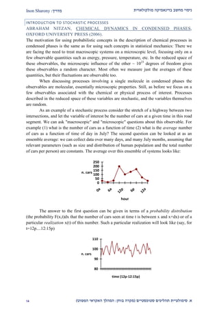
PROBABILITY THEORY AND RANDOM WALK
FREDERICK REIF, "ELEMENTARY PROBABILISTIC & STATISTICAL
CONCEPTS AND EXAMPLES" AND "THE SIMPLE RANDOM WALK IN 1-D" (PP.
4-24) IN FUNDAMENTALS OF STATISTICAL AND THERMAL PHYSICS,
MCGRAW-HILL (1965). A 2008 VERSION ALSO EXISTS.
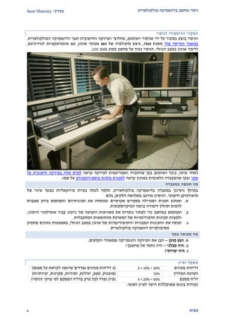
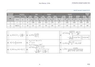
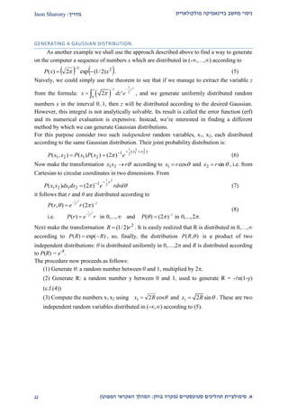
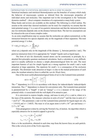
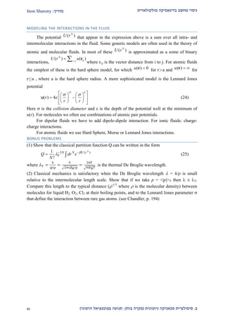
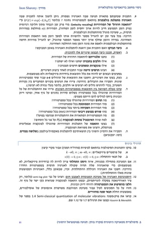
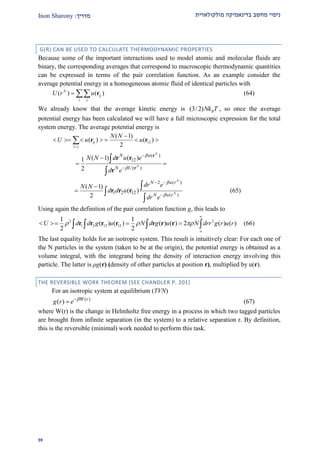
A simple example of a stochastic process associated with a reduced molecular
description is the simple random walk of a particle in one dimension. The particle goes to the
right with probability p, to the left with probability q, such that p+q=1. We want to
investigate this motion as a function of the total number of steps N.
Let n denote the number of steps taken to the right (N-n steps taken to the left). This is
a random variable. Let WN(n) denote the probability to observe the result "n" in a particular
experiment. The number of distinct walks that can give this outcome is N!/[n!(N-n)!] so that
W n
N
n N n
p qN
n N n
( )
!
!( )!



(1)
Note that W n p qN
N
n
N
( ) ( )  

 1
0
, so WN is normalized. This is the binomial distribution.
For the net number of steps to the right, m=n-(N-n)=2n-N we get
P m W n m
N
N m N m
P qN N
N m N m
( ) ( ( ))
!
( )!( )!
 
 
 
2 2
2 2
(2)
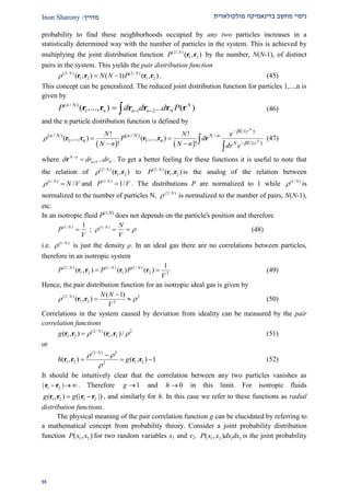
The moments Mk of a probability distribution P(m) are defined according to
Mk=<mk>= m P mk
x
 ( ) in the discrete case, or Mk=<xk>= dxx F xk
( )z for continuous
distributions. Note that M1 is the average, while the second moment M2 is related to the
variance, <x2>=M2-M1
2. These and higher moments can be calculated using the following
procedure
1
1
1
!
!( )!
!
( ) ( )
!( )!
N
n N n
n
N
n N n N N
n
N
n p q n
n N n
N
p p q p p q pN p q pN
p n N n p




 

 


     
 


(3)
2 2
1 2 2
( ) ( )
[ ( ) ( 1)( ) ] ( )
N
N N
n p p q
p
p N p q pN N p q Np Npq 

  

      
(4)
Thus the variance is
2
2 2
4 4
n Npq
m n Npq

 
 
   
(5)
For p=q=1/2 we have <m2>=N.

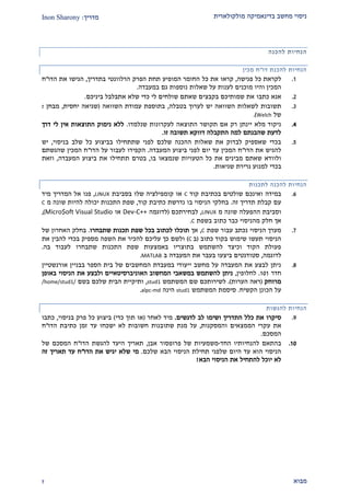
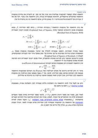
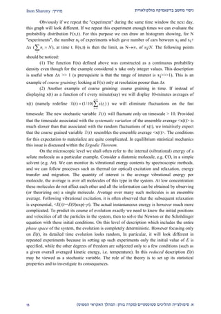
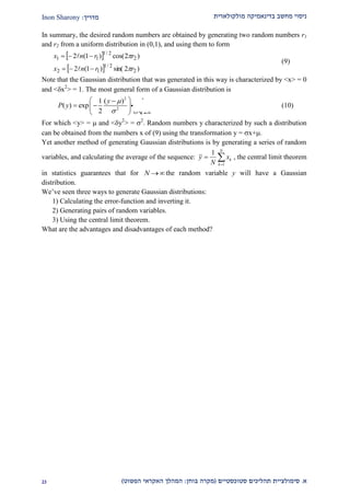
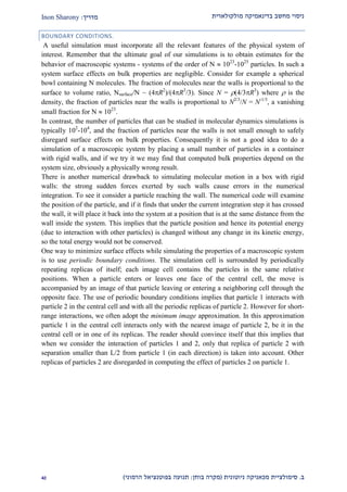
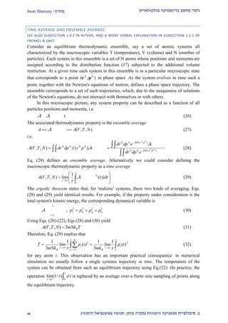
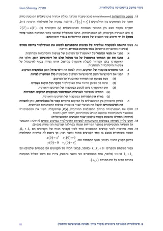
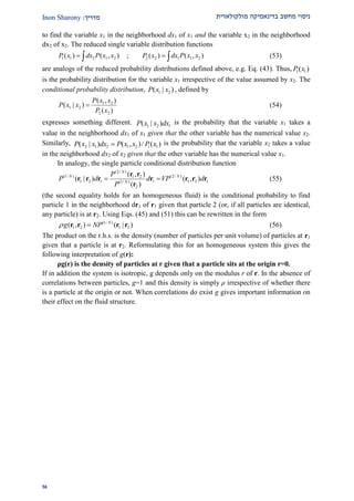
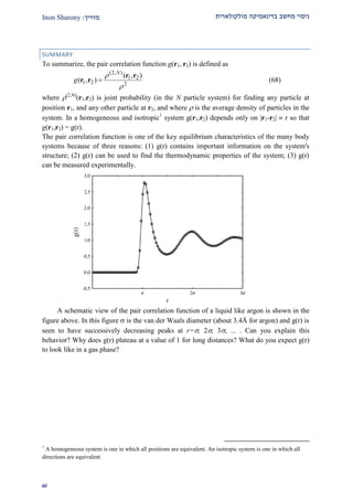
What is the relation of this result to the actual process of diffusion? In order to make
the connection let l be the step length, and  - the step time. Thus, N steps correspond to the
total elapsed time t=N, and the final distance of the particle from the origin is the random
variable x=ml. We have found that for a symmetric random walk <x2>=l2<m2>
=l2N=(l2/)t. The factor l2/ can be estimated from molecular arguments: l is expected to be
of the order of the mean free path, 1
)( 
 , where  is the molecular cross-section and  is the
density.  is of the order of the time between collisions, l/v, where v is the thermal velocity,
v= /Bk T m . This leads to l2/= /Bk T m /().
Compares this to what is obtained from the diffusion equation
2
2
2
( , ) ( , )
( , )
F x t F x t
D F x t D
t x
 
  
 
, (6)
where F(x,t) is the probability density to find the particle at x at time t. This leads to
2
2
0
x F F F
D x D x
t x xx
 
 
       
           
  (7)
provided that F0 faster than x. Similarly
2 2
2
2
2 2 2
x F F
D x D x D F D
t xx
  
  
    
    
 
   (8)
Since <x2>t=0=0 we found that <x2>t=2Dt, and, comparing to the result of the random walk
calculation, we see that if we require both formulations to yield the same result, then
D
l

2
2
(9)
Note that the random walk problem was handled in discrete space while the diffusion was
considered as a continuous process. To see the connection between the two descriptions we
can go to the continuum limit of the random walk process. This is obtained when the number
of steps becomes large while the step size l becomes much smaller than our resolution. In this
limit the factorial factors in WN(n), Eq. (1) can be approximated by the Stirling relation,
ln(N!)NlnN-N. Using this in Eq. (1) leads to
ln[ ( )] ln ln ( )ln( ) ln ( )lnW n N N n n N n N n n p N n qN         (10)
Further simplification is obtained if we expand WN
(n) about its maximum at n*. n* is
obtained from ln[W(n)]/n=0. This leads to n*=Np=<n>. The nature of this extremum is
identified as a maximum using


2
2
1 1
0
ln
( )
W
n n N n
N
n N n
  

 

 (11)
When evaluated at n* it gives )/(1|/ln *
22
NpqnW n
 .
It is important to note that higher derivatives of lnW are negligibly small if evaluated at or
near n*. For example,


3
3 2 2 2 2 2
1 1 1 1 1ln
( )
( )*
W
n n N n N p qn
 

  (12)

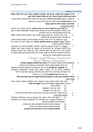
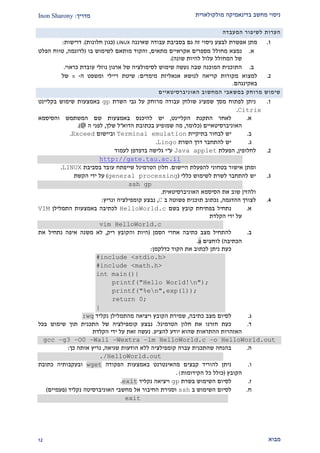
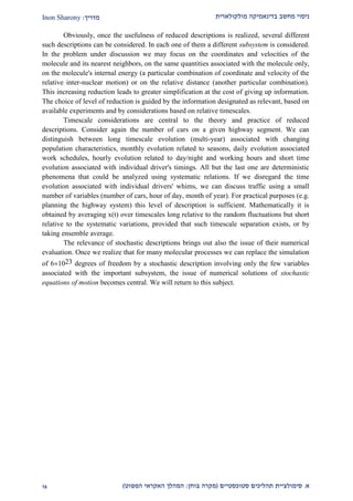
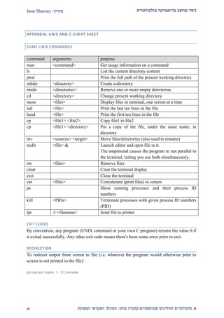
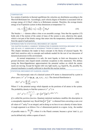
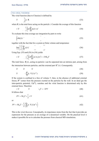
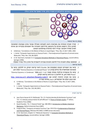
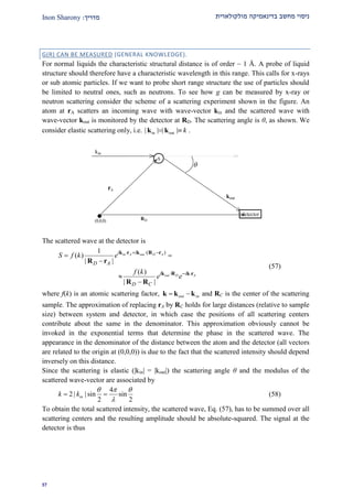
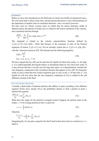
and derivatives of order k will scale as (1/N)k-1. Therefore, for large N, WN can be
approximated by truncating the expansion after the first non-vanishing, second order, term.
This yields
W n n NpN
n n
n
Ae( ) ; *
( )*
 


 
2
2
2  (13)
where the pre-exponential term can be chosen so as to make the resulting Gaussian
distribution normalized. The result (13) is an example of the Central Limit Theorem of
Probability theory. For the variable m=2n-N we get
P m W
N m
B
m N p q
Npq
B
m m
m
N N( ) ( )
exp
[ ( )]
exp
( )


 
 RST
UVW

  
 
RST
UVW
2
8 2
2 2
2

(14)
Eqs. (13) and (14) are approximations (which become practically exact for large N) to
the discrete distributions WN
(n) and PN(m). To obtain a continuous description via coarse-
graining we can average these distributions over some intervals x=lm. Accordingly we
define
F x x P m
x
P x ml
m x
( ) ( ) ( )


  

 2l
(15)
The second equality assumes that the interval x is small enough so that P(m) does not
change appreciably within this interval. The factor 2 results from the fact that only half the
integers in this interval contribute (successive values of m=2n-N differ by 2). It is very
important to keep in mind that P(m) and F(x) are different quantities (probability and
probability density) with different dimensionalities. The factor x/l, while mathematically
meaningful, has no consequence in the present discussion since the pre-exponential
coefficient is to be determined so as to satisfy normalization. Using Eq. (15) in (14) and
requesting that F(x) is normalized in the interval (-,) finally leads to
F x
p q Nl
l Npq
x
e( )
( )
( )

 


1
2
2
2
2
2
 




(16)
It is easily realized that the  and  are, respectively, the average and standard deviations of
the continuous random variable x, i.e.
F x dx( )


z 1 (17a)
xF x dx( )


z   (17b)
( ) ( )x F x dx 


z  2 2
(17c)
As expected, these results are consistent with the relations <m>=N(p-q), <m2> =4Npq, and
x=ml.

NUMERICAL SIMULATIONS OF STOCHASTIC PROCESSES
The basis of our ability to generate stochastic processes on the computer is the
possibility to use the computer as a pseudo-random number generator. It is relatively easy to
write an algorithm that will generate a sequence of “random numbers” between 0 and 1.
These are actually 'pseudo random numbers': The sequence generated by most algorithms is
completely deterministic (in the sense that if the same sequence of instructions are issued to
the computer the same sequence of numbers will be generated), and in fact periodic; however
the period is very large and for short enough sequences the numbers appear and behave as if
they are indeed random. On UNIX stations a call to the functions drand48( ) in the form
r = drand48( )
gives a number between 0 and 1, and successive calls give additional such numbers, so we
get a sequence {rn}. Defining 2/1 nn rz , this sequence appears as a set of random
numbers which are distributed uniformly in the interval
1 1
,
2 2
 
  
. The reader should identify
the random number generator on an available platform, and try to confirm the following
expectations:
 
80/1;0
121
0
43
2



zz
zzz
z
nmnmnmn  (1)
These averages can be obtained by taking an ensemble of sequences (“ensemble average”), or
along a single sequence (“time average”). Of course, a computation based on a finite
sampling will give only approximate result, for example 


N
n
nzN
1
1
give an approximation to
<z> which is better for larger N. Probability theory tells us that the error in this computation
scales as
1
2
N

.
The numbers z obtained as described above correspond to a uniform distribution
between -(1/2) and (1/2):


 

otherwise0
5.05.0;1
)(
z
zP
so that  
5.0
5.0 1)(zdzP . We saw that the computer can generate a sequence of random
numbers from this distribution. We can get a numerical plot of P(z) by dividing the interval -
0.5 …0.5 to equally spaced intervals of size z=1/N, and constructing a histogram whose
height at point n measures the number of times z is found in the interval -0.5+nz … -
0.5+(n+1)z, (n=0,…,N-1), after doing a given (large) number of “experiments” in which z is
determined. These experiments are like tossing a coin, but here the "coin", i.e. the random
number generator can show any result between -0.5 and 0.5 with equal probability.

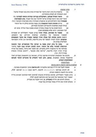
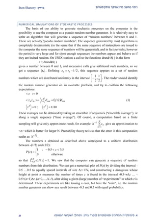
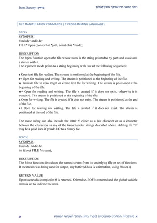
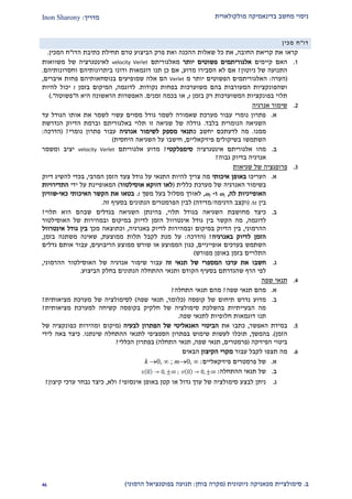
GENERATING PSEUDO-RANDOM NUMBERS FROM A GENERAL DISTRIBUTION
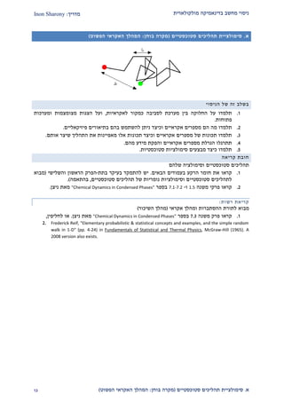
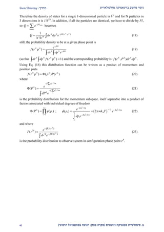
As said above, most computers provide calls to functions which generate pseudo-
random numbers r in the interval 0…1, and by simple shift and scaling we can get random
numbers distributed evenly in any interval (i.e. if r is distributed evenly in the interval [0,1],
then z=(B-A)r+A is distributed evenly in the interval [A,B]). In many applications we want to
generate random numbers whose distribution is other than uniform. For example, in order to
assign velocities to atoms in a molecular system at thermal equilibrium we need to generate
random numbers distributed according to the Maxwell-Boltzmann distribution,
    2222/3
)2/(exp)/(2),,( zyxzyx vvvmmvvvP   . The following theorem from
probability theory provides a useful method:
Let r be a random variable that is distributed uniformly in the interval 0,…,1. Let W(x) be
a nonzero function in the interval bxa  , which satisfies
1)( 
b
a
xdxW
. The random
variable z, obtained from r using the relation 
z
a
zWdzr )'('
[namely use this relation to
find z = z(r)], is distributed with the probability density: W(z)dz in the interval bza  .
The proof is simple: start from
dzzWdrzW
dz
dr
)(i.e.;)(  (2)
Together with the general relation dzzPdrrP zr )()(  between the probability distributions of
random variable r and another such variable z, obtained from r by the 1:1 mapping z=z(r), we
find
)()()( zPzWrP zr  (3)
Hence )()( zWzPz  (because 1)( rPr ) (‫משל‬) .
For example, if r is distributed uniformly in 0,…,1 and z is defined in the interval 0… by
)1()(i.e.;1'
0
'
rnrzeedzr
z
zz
 

 (4)
then the resulting z is distributed in 0…∞ according to z
z ezP 
)( .

GENERATING A GAUSSIAN DISTRIBUTION.
As another example we shall use the approach described above to find a way to generate
on the computer a sequence of numbers x which are distributed in (-,…,) according to
   21
)2/1(exp2)( xxP 

 . (5)
Naively, we could simply use the theorem to see that if we manage to extract the variable z
from the formula:  
21
1 '
2
0
2 '
zz
x dz e
 
  , and we generate uniformly distributed random
numbers x in the interval 0..1, then z will be distributed according to the desired Gaussian.
However, this integral is not analytically solvable. Its result is called the error function (erf)
and its numerical evaluation is expensive. Instead, we’re interested in finding a different
method by which we can generate Gaussian distributions.
For this purpose consider two such independent random variables, x1, x2, each distributed
according to the same Gaussian distribution. Their joint probability distribution is:
)(1
2121
2
2
2
12
1
)2()()(),(
xx
exPxPxxP

  (6)
Now make the transformation rxx 21 according to cos1 rx  and sin2 rx  , i.e. from
Cartesian to circular coordinates in two dimensions. From
 rdrdedxdxxxP
r2
2
1
1
2121 )2()(

 (7)
it follows that r and θ are distributed according to
1 2
2
1 2
2
1
1
( , ) (2 )
i.e. ( ) in 0,..., and ( ) (2 ) in 0,...,2 .
r
r
P r e r
P r e r P
 
  
 
 

  
(8)
Next make the transformation 2
)2/1( rR  . It is easily realized that R is distributed in 0,…,∞
)exp()( RRP  , so, finally, the distribution ),( RP is a product of two
independent distributions: θ is distributed uniformly in 0,…,2 and R is distributed according
to P(R) = e-R
.
The procedure now proceeds as follows:
(1) Generate θ: a random number between 0 and 1, multiplied by 2.
(2) Generate R: a random number y between 0 and 1, used to generate R = -n(1-y)
(c.f.(4))
(3) Compute the numbers x1 x2 using cos21 Rx  and 2 2 sinx R  . These are two
independent random variables distributed in (-∞,∞) according to (5).

In summary, the desired random numbers are obtained by generating two random numbers r1
and r2 from a uniform distribution in (0,1), and using them to form
 
  )2sin()1(2
)2cos()1(2
2
2/1
12
2
2/1
11
rrnx
rrnx






(9)
Note that the Gaussian distribution that was generated in this way is characterized by <x> = 0
and <x2
> = 1. The most general form of a Gaussian distribution is
2
2
1 ( ) 1
( ) exp
2 2
y
P y

  
 
  
 
(10)
For which <y> =  and <y2
> = 2
. Random numbers y characterized by such a distribution
can be obtained from the numbers x of (9) using the transformation y = x+.
Yet another method of generating Gaussian distributions is by generating a series of random
variables, and calculating the average of the sequence:
1
1 N
k
k
y x
N 
  , the central limit theorem
in statistics guarantees that for N the random variable y will have a Gaussian
distribution.
We’ve seen three ways to generate Gaussian distributions:
1) Calculating the error-function and inverting it.
2) Generating pairs of random variables.
3) Using the central limit theorem.
What are the advantages and disadvantages of each method?

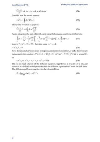
APPENDIX: HOW DOES DRAND48() WORK?
drand48() generates double-precision pseudo-random numbers that are uniformly distributed
in the interval [0..1], using a linear congruent algorithm and 48-bit integer arithmetic. It has
an internal buffer, in which it stores a 48-bit integers Xk (smaller then 2.8*1014
). Double
precision floating-point numbers between 0 and 1 are obtained from this 48-bit integer by
dividing the result by the maximal integer 248
-1. Each time drand48() is called, it generates a
new 48-bit integer Xk+1 to replace the last one by:
   48
1 mod 2k kX aX c  
(mod stands for modulus, which is the reminder in the division of two integers).
The values of the parameters a and c can be set by lcong48(), and the initial number X0 (also
called the random seed) has to be set by srand48() or seed48(). If these values are not
initialized, they assume the following default values:
a=25214903917
c=11
These numbers guarantee that the periodicity of drand48() would be very large, and that the
correlation between elements in the series would be small.
Note that while the first few moments and correlations of the pseudo-random number series
seem to indicate that it’s uncorrelated, some higher moments show that there is some
correlation, and that more complicated methods are needed to create better pseudo-random
numbers.
Bonus: How would the sequence generated by drand48() be affected by the following
changes,
I. Change a to 4
II. Change a to 224
III. Change c to 0
These changes can be effected by use of the lcong48() function.

APPENDIX: UNIX AND C CHEAT SHEET
SOME UNIX COMMANDS
command arguments purpose
man <command> Get usage information on a command
ls List the current directory content
pwd Print the full path of the present working directory
mkdir <directory> Create a directory
rmdir <directories> Remove one or more empty directories
cd <directory> Change present working directory
more <files> Display files in terminal, one screen at a time
tail <file> Print the last ten lines in the file
head <file> Print the first ten lines in the file
cp <file1> <file2> Copy file1 to file2
cp <file1> <directory> Put a copy of the file, under the same name, in
directory
mv <sources> <target> Move files/directories (also used to rename)
nedit <file> & Launch editor and open file in it.
The ampersand causes the program to run parallel to
the terminal, letting you use both simultaneously.
rm <files> Remove files
clear Clear the terminal display
exit Close the terminal
cat <files> Concatenate (print files) to screen
ps Show running processes and their process ID
numbers
kill <PIDs> Terminate processes with given process ID numbers
(PID)
lpr -l <filename> Send file to printer
EXIT CODES
By convention, any program (UNIX command or your own C program) returns the value 0 if
it exited successfully. Any other exit code means there's been some error prior to exit.
REDIRECTION
To redirect output from screen to file (i.e. whatever the program would otherwise print to
screen is not printed to the file):
program-name > filename

SOME C COMMANDS AND EXAMPLES
"FOR" LOOP
int i,max=3;
for(i=0;i<max;i++){
/* do something "max" times*/
printf("For the %d-th time, Hello World!n",i);//this line prints
"Hello World!" to screen
}
ARRAYS
int i,asize=4;
double a[asize]={0};//note that in C, the array goes from zero to asize-1
for(i=0;i<asize;i++){
a[i]=i*i;
printf("The %d-th component of the array is: a[%d]=%fn",i,i,a[i]);
}
FILE MANIPULATION
#include <stdio.h>
/*this program reads in 10 lines from input.txt (line-by-line) and writes
them to output.txt, while searching the input for integers and printing
them to screen. The program assumes no line is more than 256 characters
long*/
#define MaxBufferSize 256
#define MaxLines 10
int main(){
FILE *readFP=NULL, *writeFP=NULL;
int i,j=0;
char buffer[MaxBufferSize];
readFP=fopen("input.txt","r");
if (NULL == readFP){
fputs("Couldn't open input.txt for reading. Exiting.n",stderr);
exit(1);//exit with code 1 (not 0)
}
writeFP=fopen("output.txt","w");
if (NULL == writeFP){
fputs("Couldn't open output.txt for writing. Exiting.n",stderr);
exit(2);
}
for(i=0;i<MaxLines;i++){
fgets(buffer,MaxBufferSize,readFP);//read a single line from input.txt
and put it in the "buffer" variable
sscanf(buffer,"%d",&j);//scan for the first integer found
printf("In the %d-th linenthere appears the number %dn",i,j);
fputs(buffer,writeFP);//write to output.txt
}
return 0;//successful completion
}

ARITHMETIC, COMPARISON, LOGICAL, AND CASTING OPERATIONS
operator purpose notes
+ addition Binary operator: adds value to its right with
value on its left
- subtraction
* multiplication
/ division Gives integer part in division of integers
% modulus Gives remainder in division of integers
== check equality returns 1 if true, 0 if false
>= check greater than or equal
to
<= check less than or equal to
! negation "not"
&& conjunction "and"
|| disjunction "or"
(int) cast to integer type Changes value to its right to an integer,
discarding the non-integer part (i.e. rounds
down)
(double) cast to double type Changes value to its right to a double

GNUPLOT – A LINUX GRAPHING TOOL
You may choose to graph your data on another PC, but if you don't, you can use the
GNUPlot program, called by the command gnuplot from the terminal. This program is also
well documented. Information regarding any command can be accessed using the "help"
command. To quit gnuplot just type quit (or use the shortcut command, q).
PLOTTING TO SCREEN
set term x11
set output
# The pound sign (hash) signifies that this is a comment line
# 2-D plot command
plot "data.dat" using 1:2 with lines title "column 2 vs. 1"
# 3-D plot command
splot "data.dat" using 1:2:3 title "3 vs. 2 & 1"
PLOTTING TO FILE
set term jpeg
set output "data.jpeg"
# We can use variables, too
DataFile="data.dat"
abscissa=2
ordinate=3
set xrange [-5.3:16.8]
# p, u, w and t are shortcuts for plot, using, with and title
# The C function sprintf can be used to create formatted text
# We can plot two series of data on a single plot
p DataFile u abscissa:ordinate w linespoints t sprint("%d vs.
%d",ordinate,abscissa), 'data2.dat' u 4:ordinate t "now vs. 4"
FITTING DATA TO A FUNCTION
f(x,y,a,b)=a*cos(x)+b/y
a=5
# fitting parameters initially equal 1 unless specified
fit f(x,y,a,b) 'data.dat' using 1:2 via a,b

FILE MANIPULATION COMMANDS ( C PROGRAMMING LANGUAGE)
FOPEN
SYNOPSIS
#include <stdio.h>
FILE *fopen (const char *path, const char *mode);
DESCRIPTION
The fopen function opens the file whose name is the string pointed to by path and associates
a stream with it.
The argument mode points to a string beginning with one of the following sequences:
r Open text file for reading. The stream is positioned at the beginning of the file.
r+ Open for reading and writing. The stream is positioned at the beginning of the file.
w Truncate file to zero length or create text file for writing. The stream is positioned at the
beginning of the file.
w+ Open for reading and writing. The file is created if it does not exist, otherwise it is
truncated. The stream is positioned at the beginning of the file.
a Open for writing. The file is created if it does not exist. The stream is positioned at the end
of the file.
a+ Open for reading and writing. The file is created if it does not exist. The stream is
positioned at the end of the file.
The mode string can also include the letter 'b' either as a last character or as a character
between the characters in any of the two-character strings described above. Adding the "b''
may be a good idea if you do I/O to a binary file.
FCLOSE
SYNOPSIS
#include <stdio.h>
int fclose( FILE *stream);
DESCRIPTION
The fclose function dissociates the named stream from its underlying file or set of functions.
If the stream was being used for output, any buffered data is written first, using fflush(3).
RETURN VALUE
Upon successful completion 0 is returned. Otherwise, EOF is returned and the global variable
errno is set to indicate the error.

FREAD, FWRITE
SYNOPSIS
#include <stdio.h>
size_t fread( void *ptr, size_t size, size_t nmemb, FILE *stream);
size_t fwrite( const void *ptr, size_t size, size_t nmemb, FILE *stream);
DESCRIPTION
The function fread reads nmemb elements of data, each size bytes long, from the stream
pointed to by stream, storing them at the location given by ptr.
The function fwrite writes nmemb elements of data, each size bytes long, to the stream
pointed to by stream, obtaining them from the location given by ptr.
FSEEK
SYNOPSIS
#include <stdio.h>
int fseek( FILE *stream, long offset, int whence);
DESCRIPTION
The fseek function sets the file position indicator for the stream pointed to by stream. The
new position, measured in bytes, is obtained by adding offset bytes to the position specified
by whence. If whence is set to SEEK_SET, SEEK_CUR, or SEEK_END, the offset is
relative to the start of the file, the current position indicator, or end-of-file, respectively.
FPRINTF
SYNOPSIS
#include <stdio.h>
int printf(const char *format, ...);
int fprintf(FILE *stream, const char *format, ...);
DESCRIPTION
The functions in the printf family produce output according to a format as described below.
The function printf writes output to stdout, the standard output stream; fprintf writes output to
the given output stream.

‫דו‬"‫מכין‬ ‫ח‬
‫החובה‬ ‫קריאת‬ ‫את‬ ‫קראו‬,‫את‬‫כל‬‫הדו‬ ‫כתיבת‬ ‫תחילת‬ ‫טרם‬ ‫הביצוע‬ ‫פרק‬ ‫ואת‬ ‫ההכנה‬ ‫שאלות‬"‫המכין‬ ‫ח‬.
2.‫בשפת‬ ‫בסיסי‬ ‫תכנות‬C
‫א‬.‫קוד‬ ‫בכתיבת‬ ‫שולטים‬ ‫ואינכם‬ ‫במידה‬C‫שלו‬ ‫קומפילציה‬ ‫או‬‫בסביבת‬LINUX,‫אל‬ ‫פנו‬
‫המדריך‬‫זה‬ ‫תדריך‬ ‫קבלת‬ ‫עם‬ ‫מיד‬.
‫ב‬.‫ב‬ ‫קצרה‬ ‫תכנית‬ ‫כתבו‬C‫מהמשתמש‬ ‫שלם‬ ‫מספר‬ ‫המקבלת‬,N,‫ומציגה‬N‫שהוגרלו‬ ‫תוצאות‬
‫קובייה‬ ‫בהטלת‬ ‫באקראי‬(‫לקבלת‬ ‫שווים‬ ‫סיכויים‬2,1,2,1,2,9.)
(2)‫תקינותה‬ ‫לבדיקת‬ ‫והרצה‬ ‫קומפילציה‬ ‫בצעו‬,‫לדוגמה‬ ‫ופלט‬ ‫הקוד‬ ‫את‬ ‫והגישו‬.
(1)‫פונקציה‬ ‫כתבו‬‫המייצרת‬‫מנורמלת‬ ‫היסטוגרמה‬,‫להצגת‬ ‫בה‬ ‫והשתמשו‬
‫מחלקות‬ ‫שש‬ ‫בת‬ ‫היסטוגרמה‬(‫עמודות‬,‫או‬bins)‫הקובייה‬ ‫הטלת‬ ‫תוצאות‬ ‫עבור‬
(‫עבור‬N >> 1).
‫ביצוע‬ ‫לשם‬‫שהוגרלו‬ ‫המספרים‬ ‫כלל‬ ‫את‬ ‫לזכור‬ ‫צורך‬ ‫אין‬ ‫הבאות‬ ‫המטלות‬.
‫הדרכה‬:‫ההיסטוגרמות‬ ‫את‬ ‫אתחלו‬.‫הגרילו‬‫יחיד‬ ‫מספר‬,‫ו‬‫ההיסטוגרמות‬ ‫את‬ ‫עדכנו‬
‫שהוגרל‬ ‫למספר‬ ‫בהתאם‬.‫חזרו‬‫האחרונות‬ ‫הפעולות‬ ‫שתי‬ ‫על‬N‫פעמים‬.
‫כך‬‫הקוד‬ ‫יעילות‬ ‫את‬ ‫תשפרו‬,‫בהיבט‬ ‫הן‬‫צריכת‬‫צריכת‬ ‫בהיבט‬ ‫והן‬ ‫הזיכרון‬ ‫משאבי‬
‫החישוב‬ ‫משאבי‬(‫הריצה‬ ‫זמן‬).‫ב‬‫המשך‬‫של‬ ‫המכריע‬ ‫שברובם‬ ‫תיווכחו‬ ‫הניסוי‬
‫המקרים‬,‫חי‬‫בזכירת‬ ‫תלויים‬ ‫אינם‬ ‫שתבצעו‬ ‫שובים‬‫תוצאות‬‫חישובים‬‫קודמים‬.
(‫א‬)‫ערכי‬ ‫מה‬‫ההסתברות‬ ‫צפיפות‬‫מההיסטוגרמה‬ ‫המשתמעת‬?
(‫ב‬)‫עבור‬ ‫התהליך‬ ‫על‬ ‫חזרו‬‫קובייה‬ ‫הטלת‬ ‫תוצאות‬ ‫אותן‬,‫ציירו‬ ‫וכעת‬
‫בת‬ ‫היסטוגרמה‬‫שתיים‬/‫מחלקות‬ ‫שלוש‬(‫לבחירתכם‬).‫לדוגמה‬ ‫פלט‬ ‫הציגו‬.
‫כאשר‬‫שלמים‬ ‫שאינם‬ ‫גדלים‬ ‫של‬ ‫היסטוגרמות‬ ‫תבצעו‬(‫לדוגמה‬,‫של‬ ‫מהירויות‬
‫בקופסה‬ ‫חלקיקים‬)‫לחלק‬ ‫בהיסטוגרמה‬ ‫עמודות‬ ‫כמה‬ ‫בין‬ ‫להחליט‬ ‫תצטרכו‬
‫התחום‬ ‫את‬(‫שלנו‬ ‫בדוגמה‬,‫לכמה‬"‫מחלקות‬"‫או‬bins‫תחום‬ ‫את‬ ‫לחלק‬
‫המהירויות‬.)‫פאות‬ ‫שש‬ ‫בעלת‬ ‫קובייה‬ ‫של‬ ‫המקרה‬‫פשוט‬,‫מספיק‬ ‫אבל‬
‫שתיוצר‬ ‫ההיסטוגרמה‬ ‫על‬ ‫המחלקות‬ ‫מספר‬ ‫של‬ ‫ההשפעה‬ ‫להמחשת‬:‫הנרמול‬
‫מהמחלקות‬ ‫אחת‬ ‫לכל‬ ‫התורם‬ ‫התחום‬ ‫מגודל‬ ‫גם‬ ‫מושפע‬ ‫ההיסטוגרמה‬ ‫של‬.
‫נקרא‬ ‫אחת‬ ‫מחלקה‬ ‫תחת‬ ‫דגימות‬ ‫מספר‬ ‫ייצוג‬coarse-graining.
(‫ג‬)‫חזר‬‫ו‬‫עבור‬‫בת‬ ‫היסטוגרמה‬‫מחלקות‬ ‫חמש‬‫ההבדלים‬ ‫את‬ ‫והסבירו‬
‫ובצפיפ‬ ‫בהסתברות‬‫ההסתברות‬ ‫ות‬.‫לדוגמה‬ ‫פלט‬ ‫הציגו‬.
(2)‫פעמיים‬ ‫התכנית‬ ‫את‬ ‫הריצו‬,‫ה‬ ‫עבור‬ ‫ערך‬ ‫אותו‬ ‫עם‬seed.‫הר‬ ‫כעת‬‫יצו‬‫את‬
‫פעמיים‬ ‫התכנית‬,‫ה‬ ‫את‬ ‫שנו‬ ‫אך‬seed‫לשנייה‬ ‫הראשונה‬ ‫הריצה‬ ‫בין‬.‫ההבדל‬ ‫מה‬
‫בתוצאות‬?
‫ג‬.‫מידע‬ ‫של‬ ‫גדולות‬ ‫כמויות‬ ‫עם‬ ‫בעבודה‬,‫במקום‬ ‫בינאריים‬ ‫בקבצים‬ ‫להשתמש‬ ‫יותר‬ ‫חסכוני‬
‫טקסט‬ ‫קבצי‬,‫למ‬‫כטקסט‬ ‫אותם‬ ‫לקרוא‬ ‫ניתן‬ ‫שלא‬ ‫רות‬.‫ניתן‬ ‫שלא‬ ‫קובץ‬ ‫הוא‬ ‫בינארי‬ ‫קובץ‬
‫מבנהו‬ ‫הכרת‬ ‫ללא‬ ‫אותו‬ ‫לקרוא‬,‫אותו‬ ‫שכתבה‬ ‫התוכנית‬ ‫הכרת‬ ‫ידי‬ ‫על‬ ‫רק‬ ‫ניתן‬ ‫וזאת‬.
(2)‫חדש‬ ‫משתנה‬ ‫סוג‬ ‫הגדירו‬‫בשם‬dvector‫כמבנה‬ ‫שמורכב‬(struct)‫משלושה‬
‫רכיבים‬,‫מהם‬ ‫אחד‬ ‫כל‬‫כפול‬ ‫בדיוק‬ ‫עשרוני‬ ‫מספר‬(double.)
(‫וראו‬:http://www.tau.ac.il/~physchem/Dynamics/code/C/typedefs.h)
(1)‫הספרייה‬ ‫בפונקצית‬ ‫השתמשו‬fwrite‫ו‬‫של‬ ‫מערך‬ ‫הכותבת‬ ‫פונקציה‬ ‫כתבו‬n
‫משתני‬dvector‫בינארי‬ ‫לקובץ‬.‫שני‬ ‫מסדר‬ ‫יהיה‬ ‫שהמערך‬ ‫לב‬ ‫שימו‬:‫כל‬‫מ‬ ‫אחד‬n
‫רכיבים‬ ‫משלושה‬ ‫מורכב‬ ‫האיברים‬,‫וב‬‫סה‬"‫כ‬3n‫מספרים‬.
(2)‫הספרייה‬ ‫בפונקצית‬ ‫השתמשו‬fread‫ו‬‫הקוראת‬ ‫תכנית‬ ‫כתבו‬n‫שלשות‬
‫מספרים‬‫מערך‬ ‫לתוך‬ ‫בינארי‬ ‫מקובץ‬‫של‬n‫משתני‬dvector,‫של‬ ‫המנה‬ ‫את‬ ‫מחשבת‬
‫ה‬‫ה‬ ‫רכיב‬‫בפונקציה‬ ‫ומשתמשת‬ ‫בשני‬ ‫ראשון‬‫בסעיף‬ ‫שכתבתם‬‫הקוד‬‫ם‬‫ע‬‫ל‬‫מנת‬
‫את‬ ‫לכתוב‬‫הרכיב‬‫ה‬‫ראשון‬‫ו‬‫השני‬‫והמנה‬‫בשני‬ ‫הראשון‬ ‫של‬‫בינארי‬ ‫לקובץ‬.‫בצעו‬
‫קומפילציה‬‫תקינותה‬ ‫לבדיקת‬ ‫והרצה‬,‫ו‬‫הקוד‬ ‫את‬ ‫הגישו‬.

(1)‫הספרייה‬ ‫בפונקצית‬ ‫השתמשו‬fseek‫וכתבו‬‫פונקציה‬‫נתון‬ ‫איבר‬ ‫הקוראת‬
‫הבינארי‬ ‫מהקובץ‬‫כטקסט‬ ‫למסך‬ ‫תוכנו‬ ‫את‬ ‫ומדפיסה‬.‫זו‬ ‫בפונקציה‬ ‫השתמשו‬
‫שני‬ ‫איבר‬ ‫כל‬ ‫להדפסת‬‫הבינאר‬ ‫מהקובץ‬‫י‬‫למסך‬‫כטקסט‬.
1.‫הסתברות‬‫וסטטיסטיקה‬
‫א‬.‫מהו‬‫הגדולים‬ ‫המספרים‬ ‫חוק‬?‫היום‬ ‫בחיי‬ ‫זאת‬ ‫לראות‬ ‫ניתן‬ ‫איך‬-‫יום‬?‫למציאת‬ ‫הקשר‬ ‫מה‬
‫ממדידה‬ ‫ערך‬?‫כללי‬ ‫תיאור‬ ‫תנו‬‫עבור‬‫משתנה‬ ‫של‬ ‫וגדל‬ ‫הולך‬ ‫דגימות‬ ‫מספר‬‫המוגרל‬
‫אחידה‬ ‫מהתפלגות‬ ‫אקראית‬.
‫ב‬.‫מהו‬‫המרכזי‬ ‫הגבול‬ ‫משפט‬?‫היום‬ ‫בחיי‬ ‫זאת‬ ‫לראות‬ ‫ניתן‬ ‫איך‬-‫יום‬?‫להערכת‬ ‫הקשר‬ ‫מה‬
‫במדידה‬ ‫סטטיסטית‬ ‫שגיאה‬?‫כללי‬ ‫תיאור‬ ‫תנו‬‫עבור‬‫משתנים‬ ‫של‬ ‫וגדל‬ ‫הולך‬ ‫דגימות‬ ‫מספר‬
‫המוגרל‬‫ים‬‫מהתפלגו‬ ‫אקראית‬‫רוחב‬ ‫בעלות‬ ‫ממורכזות‬ ‫אחידות‬ ‫יות‬a‫ו‬2a.
‫ג‬.‫של‬ ‫התוחלת‬ ‫מערך‬ ‫מאחוז‬ ‫ביותר‬ ‫השונה‬ ‫ערך‬ ‫יחידה‬ ‫במדידה‬ ‫לקבל‬ ‫ההסתברות‬ ‫מה‬
‫בין‬ ‫אחיד‬ ‫באופן‬ ‫המתפלג‬ ‫משתנה‬-1‫ל‬1?‫ו‬‫מדידות‬ ‫שתי‬ ‫עבור‬?‫שתי‬ ‫של‬ ‫הממוצע‬ ‫לגבי‬ ‫מה‬
‫המדידות‬?‫מדידות‬ ‫שתי‬ ‫על‬ ‫ממוצעים‬ ‫שני‬ ‫נעשה‬ ‫אם‬(‫אחד‬ ‫כל‬),‫לקבל‬ ‫הסיכוי‬ ‫מה‬‫ממוצע‬
‫ממוצעים‬ ‫של‬‫התוחלת‬ ‫מערך‬ ‫מאחוז‬ ‫ביותר‬ ‫השונה‬?
2.‫איזו‬‫מגמה‬‫בסעיף‬ ‫לראות‬ ‫תצפו‬2‫של‬"‫הניסוי‬ ‫ביצוע‬"?
1.‫הביעו‬‫במו‬ ‫לשגיאה‬ ‫האנליטי‬ ‫הביטוי‬ ‫את‬‫ה‬ ‫מנט‬n‫של‬‫אקראי‬ ‫מספר‬ ‫התפלגות‬, n
x,‫בהינת‬‫ן‬
‫המספר‬ ‫של‬ ‫המדידה‬ ‫רזולוציית‬,x  .‫ח‬‫זרו‬‫עבור‬‫היחסית‬ ‫השגיאה‬.
‫בונוס‬ ‫שאלות‬
2.‫קראו‬‫הרשות‬ ‫קריאת‬ ‫את‬"‫מבוא‬‫לתורת‬‫ההסתברו‬‫ת‬‫ומהלך‬‫אקראי‬(‫מהלך‬‫השיכור‬)"
‫א‬.‫את‬ ‫הסבירו‬‫הקשר‬‫הדיפוזיה‬ ‫תופעת‬ ‫לבין‬ ‫המיקרוסקופי‬ ‫האקראי‬ ‫המהלך‬ ‫בין‬
‫המקרוסקופית‬(‫קבוע‬ ‫זרם‬ ‫ללא‬)?‫הדרכה‬:‫בין‬ ‫השוו‬‫משוואת‬‫של‬ ‫ההתפלגות‬‫צפיפות‬
‫בדיפוזיה‬ ‫החומר‬ ‫צפיפות‬ ‫של‬ ‫זו‬ ‫לבין‬ ‫האקראי‬ ‫מהמהלך‬ ‫שמתקבלת‬ ‫ההסתברות‬.
‫ב‬.‫העצ‬ ‫הדיפוזיה‬ ‫מקדם‬ ‫את‬ ‫העריכו‬‫מית‬(‫חלקיקים‬ ‫אותם‬ ‫של‬ ‫נוזל‬ ‫בתוך‬ ‫חלקיק‬ ‫של‬ ‫דיפוזיה‬)
‫אורך‬ ‫באמצעות‬‫הממוצע‬ ‫החופשי‬ ‫המהלך‬ ‫ומשך‬ ‫הממוצע‬ ‫החופשי‬ ‫המהלך‬.‫התוצאה‬ ‫בטאו‬
‫צפיפות‬ ‫באמצעות‬‫הנוזל‬,‫החלקיק‬ ‫מסת‬‫וה‬‫רדיוס‬‫שלו‬(‫קלסי‬ ‫פעולה‬ ‫חתך‬)‫והטמפרטורה‬.
‫ג‬.‫את‬ ‫העריכו‬‫ארגון‬ ‫של‬ ‫העצמית‬ ‫הדיפוזיה‬ ‫מקדם‬‫בצפיפות‬2.221‫לסמ‬ ‫גרם‬"‫וטמפרטורה‬ ‫ק‬
21.1‫קלווין‬‫ו‬‫דומות‬ ‫וטמפרטורה‬ ‫צפיפות‬ ‫עבור‬ ‫מהספרות‬ ‫ניסיונית‬ ‫לתוצאה‬ ‫השוו‬.
‫ארגון‬ ‫של‬ ‫וולס‬ ‫דר‬ ‫ואן‬ ‫ברדיוס‬ ‫השתמשו‬,2.22‫א‬‫ו‬‫נגסטרם‬.
9.‫הסתברות‬ ‫עוד‬(‫הקריאה‬ ‫חומר‬ ‫את‬ ‫קראו‬‫התומך‬)
‫א‬.‫הקשר‬ ‫מה‬‫המתמטי‬‫ההסתברות‬ ‫פונקצית‬ ‫בין‬,‫וההסתברות‬ ‫ההסתברות‬ ‫צפיפות‬
‫המצטברת‬?
‫ב‬.‫מתי‬‫שוות‬‫ההסתברות‬ ‫וצפיפות‬ ‫ההסתברות‬?
‫ג‬.‫מהו‬‫קומולנט‬?‫מה‬‫ן‬‫ה‬‫המ‬ ‫משוואות‬‫קשר‬‫ות‬‫למומנט‬ ‫קומולנט‬ ‫בין‬?
‫ד‬.‫הגדר‬‫מהי‬‫פונקציה‬‫יוצרת‬‫של‬‫התפלגות‬,‫ו‬‫ה‬‫קשר‬‫בין‬‫ה‬‫פונקציה‬‫ה‬‫יוצרת‬‫למומנט‬‫כלשהו‬.
‫ה‬.‫התפלגות‬ ‫של‬ ‫הראשונים‬ ‫המומנטים‬ ‫שני‬ ‫על‬ ‫לומר‬ ‫ניתן‬ ‫מה‬‫לורנציאנית‬?‫לראות‬ ‫ניתן‬ ‫איך‬
‫היום‬ ‫בחיי‬ ‫זאת‬-‫יום‬?‫מה‬‫ו‬,‫כך‬ ‫אם‬,‫שיתקבל‬ ‫הערך‬‫מ‬‫מדיד‬‫רבות‬ ‫ות‬‫תהליך‬ ‫של‬‫לוונציאני‬?
‫ו‬.‫בין‬ ‫אחידה‬ ‫שהתפלגותו‬ ‫משתנה‬ ‫של‬ ‫הרביעי‬ ‫שהמומנט‬ ‫הוכח‬-1/2‫ל‬1/2‫ל‬ ‫שווה‬1/80,
‫האי‬ ‫המומנטים‬ ‫ושכל‬-‫אפס‬ ‫שווים‬ ‫שלו‬ ‫זוגיים‬.
‫ז‬.‫להסתברות‬ ‫סטטיסטיקה‬ ‫בין‬ ‫הקשר‬ ‫מה‬?‫מהו‬regression analysis?

‫ח‬.‫מהו‬‫בר‬ ‫מרווח‬-‫סמך‬(confidence interval)?
(2)‫בת‬ ‫קבוצה‬ ‫של‬ ‫הממוצעת‬ ‫המשכל‬ ‫שמנת‬ ‫טוען‬ ‫מחקר‬20,000‫נמוכה‬ ‫מעשנים‬
‫בת‬ ‫מקבוצה‬ ‫נקודות‬ ‫בשבע‬20,000‫מעשנים‬ ‫שאינם‬.‫כלשהי‬ ‫שבקבוצה‬ ‫הסיכוי‬ ‫מה‬
‫בת‬20,000‫אנשים‬(‫מעשנים‬ ‫מהם‬ ‫מי‬ ‫אם‬ ‫לדעת‬ ‫מבלי‬)‫הממוצעת‬ ‫המשכל‬ ‫מנת‬
‫תהיה‬202(‫או‬22)?‫מ‬ ‫התפלגות‬ ‫לגבי‬ ‫שעשיתם‬ ‫ההנחות‬ ‫כל‬ ‫את‬ ‫הבהירו‬‫נת‬
‫המשכל‬.
(1)‫מתפלגת‬ ‫המשכל‬ ‫מנת‬ ‫הכללית‬ ‫האוכלוסייה‬ ‫שעבר‬ ‫בהינתן‬‫נורמאלי‬‫ת‬‫עם‬
‫ממוצע‬μ‫תקן‬ ‫וסטיית‬,‫בגודל‬ ‫סופי‬ ‫מדגם‬ ‫שעבור‬ ‫הסיכוי‬ ‫מה‬N‫המשכל‬ ‫מנת‬
‫תהיה‬ ‫הממוצעת‬x?‫הכללי‬ ‫המקרה‬ ‫עבור‬ ‫פתרו‬(‫ש‬ ‫להניח‬ ‫ניתן‬x‫חיובי‬)‫ועבור‬
‫בו‬ ‫המקרה‬μ =100‫ו‬=16.
‫ט‬.‫הקורלציה‬ ‫מדוע‬ ‫הסבירו‬(correlation)‫המשותפת‬ ‫לשונות‬ ‫שווה‬(covariance),‫נתון‬ ‫אם‬
‫אפס‬ ‫ואינה‬ ‫מוגדרת‬ ‫מהמשתנים‬ ‫אחד‬ ‫כל‬ ‫של‬ ‫שהשונות‬.
2.‫מהי‬point spread function(PSF)?‫הקשר‬ ‫מה‬‫המתמטי‬‫שלה‬‫ל‬‫התמסורת‬ ‫פונקצית‬‫האופטית‬(OTF)?
‫בי‬ ‫המתמטי‬ ‫הקשר‬ ‫את‬ ‫נסחו‬‫ה‬ ‫ן‬PSF‫לבין‬‫מושג‬‫הקונבולוציה‬.
2.‫סטוכסטיי‬ ‫תהליכים‬ ‫סימולציית‬‫ם‬
‫א‬.‫מספר‬ ‫שונה‬ ‫במה‬‫פסיאוד‬‫ו‬-‫מרנדומי‬ ‫רנדומי‬?‫זניח‬ ‫יהיה‬ ‫שההבדל‬ ‫כדי‬ ‫לעשות‬ ‫ניתן‬ ‫מה‬?
‫ב‬.‫ערכו‬‫טבלת‬‫השוואה‬‫של‬‫הבאות‬ ‫מהשיטות‬ ‫אחת‬ ‫כל‬ ‫של‬ ‫והחסרונות‬ ‫היתרונות‬‫להגרלת‬
‫התפלגות‬ ‫שייצרו‬ ‫מספרים‬‫נורמאלית‬(‫פעמון‬ ‫התפלגות‬/‫גאוסית‬):
(2)‫חישוב‬error function‫והיפוכה‬.
(1)‫א‬ ‫משתנים‬ ‫של‬ ‫זוגות‬ ‫הגרלת‬‫אחידה‬ ‫מהתפלגות‬ ‫קראיים‬(‫טרנספורם‬Box-
Muller).
(2)‫ב‬ ‫שימוש‬‫המרכזי‬ ‫הגבול‬ ‫משפט‬.
‫ג‬.‫החלפת‬ ‫אופן‬ ‫את‬ ‫הקובעת‬ ‫טמפרטורה‬ ‫ידי‬ ‫על‬ ‫מאופיינת‬ ‫אנרגיה‬ ‫למעבר‬ ‫פתוחה‬ ‫מערכת‬
‫לסביבה‬ ‫המערכת‬ ‫בין‬ ‫האנרגיה‬.‫הציעו‬‫אלגוריתם‬‫סטוכסטי‬(‫דטרמיניסטי‬ ‫לא‬)!‫לשימור‬
‫אנרגיה‬ ‫שמחליף‬ ‫חופשי‬ ‫חלקיק‬ ‫עבור‬ ‫טמפרטורה‬‫נתונה‬ ‫בטמפרטורה‬ ‫סביבה‬ ‫עם‬.
‫ד‬.‫המשותפת‬ ‫השונות‬ ‫מדוע‬ ‫הסבירו‬‫העצמית‬(auto covariance)‫הצולבת‬ ‫לקורלציה‬ ‫שווה‬
‫העצמית‬(auto cross correlation)‫ו‬ ‫ממשיים‬ ‫תהליכים‬ ‫עבור‬‫סטציונאריים‬,‫ו‬‫מדוע‬
‫הקונבולוציה‬(convolution)‫ל‬ ‫שווה‬‫ה‬ ‫של‬ ‫הראי‬ ‫תמונת‬‫הצולבת‬ ‫קורלציה‬(cross correlation)
‫ע‬‫בו‬‫תהליכים‬ ‫ר‬‫כאלה‬.
2.‫התדריך‬ ‫של‬ ‫זה‬ ‫בפרק‬ ‫טעויות‬ ‫גיליתם‬ ‫אם‬(‫ביצוע‬ ‫או‬ ‫הכנה‬),‫בבונוס‬ ‫לזכות‬ ‫מנת‬ ‫על‬ ‫כאן‬ ‫פרטו‬!

‫הניסוי‬ ‫ביצוע‬
‫האקראיים‬ ‫המספרים‬ ‫יוצר‬(‫רנדומיים‬)‫בשפת‬C‫במערכות‬UNIX‫הוא‬drand48().‫שלו‬ ‫הפלט‬‫הוא‬‫מספר‬
‫אקראי‬‫בין‬0‫ל‬-2,‫ו‬‫מספרים‬ ‫מניב‬ ‫בו‬ ‫חוזר‬ ‫שימוש‬‫המ‬‫ת‬‫בא‬ ‫פלגים‬‫אחיד‬ ‫ופן‬.
2.‫מומנטים‬‫האחידה‬ ‫ההתפלגות‬ ‫של‬
‫א‬.‫הראשונים‬ ‫המומנטים‬ ‫שלושת‬ ‫את‬ ‫חשבו‬‫של‬‫ההתפלגות‬‫הרנדומית‬‫האחידה‬,‫כלומר‬
‫חשבו‬:
 n
1
1
r
N n
n j
j
m r
N 
   
‫כאשר‬  1
N
j j
r

‫מספרים‬ ‫של‬ ‫סדרה‬ ‫היא‬‫אקראיים‬,‫ו‬10,100,1000,10000N .
‫ב‬.‫חשבו‬‫את‬‫הדיוק‬(precision)‫בחיש‬‫מהמומנטים‬ ‫אחד‬ ‫כל‬ ‫וב‬:‫הסטטיסטי‬ ‫הפיזור‬ ‫את‬ ‫הציגו‬,
‫התקן‬ ‫סטיית‬ ‫כלומר‬(N)‫המדגמים‬ ‫מגדלי‬ ‫אחד‬ ‫כל‬ ‫עבור‬.
‫ג‬.‫את‬ ‫השוו‬‫הנכונות‬(accuracy)‫ה‬ ‫של‬‫תוצאות‬‫ביחס‬‫האנליטי‬ ‫לחישוב‬‫עבור‬N  ,
‫לפיו‬1 2 3
1 1 1
2 3 4
m m m  .‫המוחלטת‬ ‫השגיאה‬ ‫את‬ ‫בטאו‬()‫ה‬ ‫השגיאה‬ ‫או‬‫יחסית‬
(,‫באחוזים‬ ‫מבוטאת‬.)
 
11 1 1
0 0 0
1 0 1
1
1 1 1 1
n
n n
n
r
m r P r dr r dr
n n n n


           
 
‫ד‬.‫הש‬‫חישוב‬ ‫באמצעות‬ ‫והנכונות‬ ‫הדיוק‬ ‫את‬ ‫וו‬‫ההתאמה‬ ‫מבחן‬t‫של‬Welch,‫והפיקו‬
‫משמעויות‬:
1.‫מומנט‬ ‫איזה‬ ‫עבור‬‫ביותר‬ ‫הקטנות‬ ‫השגיאות‬ ‫מגמתי‬ ‫באופן‬ ‫מתקבלות‬?‫הסבירו‬.
2.‫היחסית‬ ‫השגיאה‬ ‫את‬ ‫ציירו‬(N,‫בשאלה‬ ‫שנמדדו‬ ‫הגדלים‬ ‫בין‬ ‫ההפרש‬ ‫כלומר‬2‫א‬'‫שניתנו‬ ‫אלו‬ ‫לבין‬
‫בשאלה‬2‫ב‬,'‫הנתונים‬ ‫בגדלים‬ ‫מחולק‬)‫כפ‬‫הדגימות‬ ‫מספר‬ ‫של‬ ‫ונקציה‬,N,(‫המדגמים‬ ‫שלושת‬ ‫עבור‬
‫יותר‬ ‫הגדולים‬),‫מהמומנטים‬ ‫אחד‬ ‫כל‬ ‫עבור‬.‫כשלוש‬ ‫המומנטים‬ ‫שלושת‬ ‫עבור‬ ‫התוצאות‬ ‫את‬ ‫הציגו‬
‫צירים‬ ‫בעל‬ ‫יחיד‬ ‫גרף‬ ‫גבי‬ ‫על‬ ‫נתונים‬ ‫סדרות‬‫בסקאלו‬‫ת‬‫לוגריתמי‬‫ו‬‫ת‬,‫ו‬‫לפונקציה‬ ‫התאמה‬ ‫בצעו‬
‫זה‬ ‫גרף‬ ‫על‬ ‫ישר‬ ‫כקו‬ ‫שנראית‬.
‫א‬.‫פונק‬ ‫נבחרה‬ ‫מדוע‬ ‫הסבירו‬‫זו‬ ‫התאמה‬ ‫צית‬.
‫לב‬ ‫שימו‬‫הראשון‬ ‫המומנט‬ ‫עבור‬ ‫המדידות‬ ‫סדרת‬ ‫של‬ ‫החיתוך‬ ‫שנקודת‬(‫בלבד‬)‫ציר‬ ‫עם‬‫האורדינאטה‬
‫לנו‬ ‫ידועה‬:‫יחידה‬ ‫מדידה‬ ‫עבור‬,‫ההתפלגות‬ ‫של‬ ‫התקן‬ ‫סטיית‬ ‫הנו‬ ‫הסטטיסטית‬ ‫השגיאה‬ ‫אומד‬
‫שנדגמה‬.‫לכן‬,‫עם‬ ‫החיתוך‬ ‫נקודת‬‫האורדינאטה‬‫של‬ ‫חופשי‬ ‫פרמטר‬ ‫היא‬‫פונקצית‬‫עבור‬ ‫רק‬ ‫ההתאמה‬
‫יותר‬ ‫הגבוהים‬ ‫המומנטים‬.
‫ב‬.‫מה‬‫שיפוע‬‫הקו‬‫המתקבל‬?

1.‫אקר‬ ‫מספר‬ ‫הגרילו‬‫אי‬,r,‫ש‬ ‫האקספוננט‬ ‫את‬ ‫וחשבו‬‫לו‬,r
e( .‫לב‬ ‫שימו‬‫שב‬-C‫להוסיף‬ ‫צורך‬ ‫יש‬
‫לתוכני‬‫ת‬"include <math.h>"‫הקומפילצי‬ ‫לפקודת‬ ‫להוסיף‬ ‫ויש‬ ‫כך‬ ‫לשם‬‫ה‬"-lm",‫לספריית‬ ‫לינק‬
‫המתמטי‬‫קה‬.)‫על‬ ‫חיזרו‬‫תרג‬‫יל‬2‫ש‬ ‫והראו‬ ‫האקספוננט‬ ‫עבור‬‫עבור‬
 
         
1 1
exp
1 expdz
dr
z r
P z dz P r dr dr P z r z
 

       
‫מתקיים‬
 
 
 1
exp 1
0 1 1
1 1
ez r e n n n
n n
n
z r
z e e
m z P z dz z z dz
n n n n



 
     

 
‫ה‬‫שורה‬‫האמצעית‬‫נובעת‬‫מ‬‫ההסתברות‬ ‫שימור‬‫ב‬‫מ‬‫מסוים‬ ‫קטע‬,.
‫מספרים‬ ‫להגרלת‬ ‫זו‬ ‫טכניקה‬‫אקראיים‬‫נקרא‬ ‫כללית‬ ‫התפלגות‬ ‫בעלי‬‫ההיפוך‬ ‫שיטת‬.
2.‫ב‬ ‫השתמשו‬‫טרנספורם‬Box-Muller‫ו‬‫תכנית‬ ‫כתבו‬‫שמגרילה‬‫רנדומיים‬ ‫מספרים‬‫מ‬‫ההתפלגות‬
‫הסטנדרטית‬ ‫הנורמאלית‬(‫ממוצע‬0‫ושונות‬2).
‫א‬.‫משתנה‬ ‫מדוע‬z‫שפשוט‬‫מוגדר‬
21
2
r
z e

(‫עם‬r‫אחידה‬ ‫מהתפלגות‬ ‫מוגרל‬,‫בדומה‬‫לתרגיל‬
2)‫לא‬‫בולצמנית‬ ‫מתפלג‬?
‫ב‬.‫תרג‬ ‫על‬ ‫חזרו‬‫יל‬2‫הנורמאלית‬ ‫מההתפלגות‬ ‫שהגרלתם‬ ‫המספרים‬ ‫עבור‬.
‫ג‬.‫נורמאלית‬ ‫להתפלגות‬ ‫המתאימה‬ ‫צורה‬ ‫שמתקבלת‬ ‫איכותי‬ ‫באופן‬ ‫וודאו‬ ‫היסטוגרמה‬ ‫ציירו‬.
9.‫בין‬ ‫הקורלציה‬‫שני‬‫האקראיים‬ ‫המשתנים‬rj , ri‫ע‬ ‫מוגדרת‬"‫י‬
  222 2
i j i jij
ij
i j
i i j j
rr r r
r r r r


 

 
 
‫קריטריו‬‫ן‬‫ל‬RNG‫טוב‬‫שהוא‬ ‫הוא‬‫מספרים‬ ‫יוצר‬‫קורלציה‬ ‫חסרי‬.‫את‬ ‫בדקו‬‫ה‬-RNG‫שלכם‬:
‫א‬.‫אם‬  1
N
j j
r

‫היא‬‫סדרה‬‫של‬‫מספרים‬‫אקראיים‬‫שנוצרה‬‫ע‬"‫י‬‫ה‬RNG,
‫חשבו‬‫א‬‫ת‬‫שונות‬‫הצולבת‬1
1
N k
k i i kN k i
C rr

 
 .
‫ב‬.‫עבור‬‫כמה‬‫ערכי‬‫ם‬‫של‬N,‫הציגו‬‫את‬Ck‫כפונקציה‬‫של‬k,‫ו‬‫הראו‬‫ש‬1lim
4k
N
C

‫עבור‬‫כל‬k
‫ש‬‫הוא‬.‫הסבירו‬‫מה‬‫עבור‬ ‫קורה‬‫ערכי‬N/k‫לאחד‬ ‫השואפים‬.
‫ג‬.‫זו‬ ‫תוצאה‬ ‫מדוע‬‫אקוויוולנטית‬‫לדרישה‬0ij ?
2.‫במערך‬ ‫אותה‬ ‫ושימרו‬ ‫אקראיים‬ ‫מספרים‬ ‫של‬ ‫סדרה‬ ‫הגרילו‬  1
N
j j
r

.‫הממוצעים‬ ‫סדרת‬ ‫את‬ ‫חשבו‬
‫הבאים‬:qj = ( rj + rj+1 ) / 2.‫על‬ ‫עבורם‬ ‫חזרו‬‫תרגיל‬2‫ו‬-2‫ל‬ ‫והשוו‬‫האנליטיות‬ ‫תוצאות‬‫עבור‬
‫החדשים‬ ‫המשתנים‬.(‫ה‬‫דרכה‬:‫האנליטי‬ ‫חישובכם‬ ‫את‬ ‫הציגו‬,‫אינסופי‬ ‫מגדם‬ ‫של‬ ‫לגבול‬ ‫השקול‬,‫של‬
‫של‬ ‫כפונקציה‬ ‫הצולבת‬ ‫השונות‬ ‫ושל‬ ‫השונים‬ ‫המומנטים‬k)
‫תרגיל‬‫בונוס‬
2.‫המרכזי‬ ‫הגבול‬ ‫משפט‬ ‫פי‬ ‫על‬ ‫לצפי‬ ‫ההתפלגויות‬ ‫של‬ ‫ההתכנסות‬ ‫קצב‬ ‫את‬ ‫השוו‬(‫להזכירכם‬,‫המשפט‬
‫מתייח‬‫ס‬‫להתכנסות‬‫בלבד‬ ‫הראשון‬ ‫המומנט‬ ‫של‬.)‫הדרכה‬:‫התפלגות‬ ‫כל‬ ‫עבור‬,‫של‬ ‫הגרף‬ ‫את‬ ‫ציירו‬
‫לוג‬ ‫גרף‬ ‫על‬ ‫המדגם‬ ‫גודל‬ ‫כנגד‬ ‫המוחלטת‬ ‫השגיאה‬-‫לו‬‫שנראית‬ ‫אנאליטית‬ ‫לפונקציה‬ ‫התאמה‬ ‫ובצעו‬ ‫ג‬
‫זה‬ ‫גרף‬ ‫על‬ ‫ישר‬ ‫כקו‬.‫ערכו‬ ‫כעת‬‫טבלת‬‫השיפועים‬ ‫בין‬ ‫השוואה‬(‫חצי‬ ‫למינוס‬ ‫קרוב‬ ‫הכי‬ ‫מי‬?)‫הסבירו‬.
2.‫של‬ ‫הערך‬ ‫חישוב‬‫הזריקה‬ ‫בשיטת‬:‫ברדיוס‬ ‫מעגל‬ ‫לחסום‬ ‫ניתן‬r‫צלע‬ ‫בעל‬ ‫ריבוע‬ ‫בתוך‬2r.
‫הריבוע‬ ‫שטח‬4r
2
‫המעגל‬ ‫ושטח‬r
2
.‫שנקודה‬ ‫ההסתברות‬‫שנבח‬‫באקראי‬ ‫רה‬‫הריבוע‬ ‫בתוך‬‫תימצא‬‫גם‬
‫היא‬ ‫המעגל‬ ‫בתוך‬/4.
‫א‬.‫גדול‬ ‫מספר‬ ‫הגרילו‬(N)‫שיהוו‬ ‫מספרים‬ ‫זוגות‬ ‫של‬‫קואורדינאטו‬‫ת‬‫ה‬x‫וה‬y‫בתוך‬ ‫נקודות‬ ‫של‬
‫בעל‬ ‫ריבוע‬r=1.
‫ב‬.‫נקודה‬ ‫כל‬ ‫עבור‬,‫לראשית‬ ‫ביחס‬ ‫שהוגרלה‬ ‫הנקודה‬ ‫מרחק‬ ‫את‬ ‫חשבו‬(‫את‬ ‫כלומר‬‫הרדיוס‬.)

‫ג‬.‫הקטן‬ ‫במרחק‬ ‫נמצאת‬ ‫הנקודה‬ ‫אם‬‫מ‬2‫מהר‬‫השל‬ ‫המספר‬ ‫את‬ ‫הגדילו‬ ‫אשית‬‫ם‬M.
‫ד‬.‫היחס‬M/N(‫ה‬‫גם‬ ‫נקרא‬"‫הקבלה‬ ‫יחס‬"‫או‬"acceptance ratio")‫ליחס‬ ‫יישאף‬/4‫עבור‬N
‫לאינסוף‬ ‫השואף‬.‫של‬ ‫ערכו‬ ‫את‬ ‫לחלץ‬ ‫ניתן‬‫כ‬4M/N‫בגבול‬N  ∞.
‫נקראת‬ ‫זו‬ ‫שיטה‬"‫הזריקה‬ ‫שיטת‬"‫או‬"rejection method"‫חצים‬ ‫לזריקת‬ ‫שקולה‬ ‫שהיא‬ ‫מכיוון‬
(darts)‫לעבר‬‫הריבוע‬ ‫בתוך‬ ‫שנפלו‬ ‫האבנים‬ ‫כלל‬ ‫וספירת‬ ‫בריבוע‬ ‫החסום‬ ‫מעגל‬ ‫בצורת‬ ‫מטרה‬(N)
‫המעגל‬ ‫ובתוך‬(M),‫התחום‬ ‫בכל‬ ‫אחיד‬ ‫שהפיזור‬ ‫ההנחה‬ ‫תוך‬.‫גם‬ ‫לחשב‬ ‫בשיטה‬ ‫משתמשים‬
‫השטח‬ ‫מחישוב‬ ‫יותר‬ ‫מורכבים‬ ‫אינטגרלים‬,‫של‬ ‫מאלו‬ ‫יותר‬ ‫מורכבים‬ ‫אינטגרציה‬ ‫גבולות‬ ‫ועם‬
‫מעגל‬,‫גם‬ ‫נקראת‬ ‫והיא‬"‫קרלו‬ ‫מונה‬"‫עקב‬‫בה‬ ‫הכרוך‬ ‫הרנדומי‬ ‫האלמנט‬.
20.‫השיכור‬ ‫מהלך‬
‫א‬.‫סימטרי‬ ‫אקראי‬ ‫מהלך‬ ‫של‬ ‫סימולציה‬ ‫המבצעת‬ ‫תוכנית‬ ‫כתבו‬‫אחד‬ ‫בממד‬:‫זמן‬ ‫צעד‬ ‫בכל‬
‫מספר‬ ‫מוגרל‬,r.‫גדול‬ ‫המספר‬ ‫אם‬‫מ‬q = 0.5,‫ימינה‬ ‫אחד‬ ‫צעד‬ ‫נעה‬ ‫המערכת‬,‫אחרת‬
‫שמאלה‬.
‫ב‬.‫הזמן‬ ‫של‬ ‫כפונקציה‬ ‫המערכת‬ ‫מיקום‬ ‫של‬ ‫גרף‬ ‫שרטטו‬.‫מה‬‫המיקום‬ ‫ו‬‫הממוצע‬?
‫ג‬.‫ג‬ ‫שרטטו‬‫של‬ ‫רף‬‫הזמן‬ ‫של‬ ‫כפונקציה‬ ‫המערכת‬ ‫שעברה‬ ‫המרחק‬ ‫ריבוע‬.‫התאמה‬ ‫לבצע‬ ‫נסו‬
‫אנליטית‬ ‫לפונקציה‬,‫את‬ ‫והסבירו‬ ‫הפונקציה‬ ‫משוואת‬ ‫את‬ ‫הציגו‬‫המשמעות‬‫הפיזיקאלי‬‫ת‬
‫מהפרמטרים‬ ‫אחד‬ ‫כל‬ ‫של‬‫בה‬ ‫המופיעים‬.
‫ד‬.‫צעדים‬ ‫של‬ ‫רב‬ ‫מספר‬ ‫בעל‬ ‫מסלול‬ ‫עבור‬,‫של‬ ‫היסטוגרמה‬ ‫שרטטו‬‫את‬ ‫למצוא‬ ‫ההסתברות‬
‫במקום‬ ‫המערכת‬‫מסו‬‫ים‬,P(x).‫אנליטית‬ ‫לפונקציה‬ ‫התאמה‬ ‫לבצע‬ ‫נסו‬,‫משוואת‬ ‫את‬ ‫הציגו‬
‫הפונקציה‬‫והסבירו‬‫תוצאתכם‬ ‫את‬.‫התאמתם‬ ‫אותה‬ ‫האנליטית‬ ‫שהפונקציה‬ ‫הראו‬‫מקיימת‬
‫תנאי‬ ‫את‬‫הנרמול‬.‫הערה‬:‫מנורמלת‬ ‫הסתברות‬ ‫לקבל‬ ‫כדי‬,‫לחלק‬ ‫יש‬‫הקריאות‬ ‫מספר‬ ‫את‬
‫תא‬ ‫בכל‬‫הת‬ ‫וברוחב‬ ‫הכולל‬ ‫הצעדים‬ ‫במספר‬‫א‬.
‫ה‬.‫ש‬ ‫סימולציה‬ ‫בצעו‬‫ל‬M‫אקראיים‬ ‫מהלכים‬‫בלתי‬-‫תלויים‬‫למשך‬N‫זמן‬ ‫צעדי‬(‫הריצו‬M
‫פעמים‬‫ה‬ ‫ערך‬ ‫את‬ ‫משנים‬ ‫אתם‬ ‫כאשר‬seed‫פעם‬ ‫בכל‬,‫את‬ ‫ומצעו‬M‫ההיסטוגרמות‬
‫המתקבלות‬.)‫באורך‬ ‫אחת‬ ‫סימולציה‬ ‫בצעו‬ ‫כעת‬MxN‫זמן‬ ‫צעדי‬.‫ההיסטוגרמה‬ ‫בין‬ ‫השוו‬
‫על‬ ‫הממוצעת‬M‫שעבר‬ ‫האחד‬ ‫המהלך‬ ‫עבור‬ ‫ההיסטוגרמה‬ ‫לבין‬ ‫מהלכים‬MxN‫צעדים‬(‫קחו‬
‫לפחות‬N=M=100‫או‬N=2M=100.)‫המסקנה‬ ‫מה‬?
‫ו‬.‫כיצד‬‫הקודמים‬ ‫מהסעיפים‬ ‫אחד‬ ‫לכל‬ ‫תשובתכם‬ ‫תשתנה‬‫של‬ ‫ערכו‬ ‫את‬ ‫נשנה‬ ‫אם‬q?

22.‫הפונקציה‬lcong48‫בהגדרות‬ ‫שולטת‬‫האקראיים‬ ‫המספרים‬ ‫יוצר‬,drand48‫האפשרות‬ ‫מתן‬ ‫ידי‬ ‫על‬
‫ה‬ ‫המספר‬ ‫את‬ ‫המייצרת‬ ‫הרקורסיה‬ ‫במשוואת‬ ‫הקבועים‬ ‫את‬ ‫לקבוע‬‫פס‬‫אודו‬-‫הבא‬ ‫אקראי‬.‫הפונקציה‬
‫כקלט‬ ‫מערך‬ ‫מקבלת‬,‫הקודם‬ ‫האקראי‬ ‫המספר‬ ‫את‬ ‫המגדיר‬(‫הזרע‬ ‫או‬)‫של‬ ‫הפרמטרים‬ ‫ואת‬‫משוואת‬
‫הרקורסיה‬(a‫ו‬-c‫הרקע‬ ‫בחומר‬ ‫במשוואה‬.)‫לפונקציה‬ ‫קריאה‬srand48()‫או‬seed48()‫את‬ ‫מאפסת‬
‫שערכה‬ ‫השינויים‬lcong48().
‫א‬.‫שבאמצעות‬ ‫הראו‬lcong48()‫אופ‬ ‫את‬ ‫לשנות‬ ‫ניתן‬‫הפסאודו‬ ‫המספר‬ ‫ייצור‬ ‫ן‬-‫הבא‬ ‫אקראי‬,
‫ואף‬‫ברצף‬ ‫הבאים‬ ‫המספרים‬ ‫את‬ ‫לנבא‬.
‫ב‬.‫פסאודו‬ ‫מספרים‬ ‫לייצור‬ ‫נוספות‬ ‫פונקציות‬ ‫הדגימו‬-‫רנדומאליי‬‫ם‬:
(2)‫הפונקציה‬random()(‫המתאים‬ ‫הזרע‬ ‫ויוצר‬,srandom())‫פסאודו‬ ‫מספר‬ ‫מחזירה‬-
‫לקבוע‬ ‫אפס‬ ‫בין‬ ‫שלם‬ ‫אקראי‬RAND_MAX.
(1)‫הפקודה‬openssl rand –hex $NUM‫מחז‬‫ירה‬NUM$‫בפורמט‬ ‫אקראיים‬ ‫בייטים‬
‫הקסאדצימלי‬.‫מחומרה‬ ‫או‬ ‫מקובץ‬ ‫לוקחת‬ ‫היא‬ ‫הזרע‬ ‫את‬,‫שמחוללים‬‫אקראי‬ ‫זרע‬.

‫ב‬.‫סימולצי‬‫ית‬‫מכאני‬‫ניוטונית‬ ‫קה‬(‫בוחן‬ ‫מקרה‬:‫הרמוני‬ ‫בפוטנציאל‬ ‫תנועה‬)22
‫ב‬.‫סימולצי‬‫ית‬‫מכאני‬‫ניוטונית‬ ‫קה‬(‫בוחן‬ ‫מקרה‬:‫הרמוני‬ ‫בפוטנציאל‬ ‫תנועה‬)
2.‫תלמדו‬‫ב‬ ‫להשתמש‬‫המילטון‬ ‫משוואות‬‫לתיאו‬‫ר‬‫הפאזה‬ ‫במרחב‬ ‫מערכת‬ ‫של‬ ‫דינאמיקה‬.
1.‫תל‬‫מדו‬‫לבצע‬‫ניוטון‬ ‫של‬ ‫התנועה‬ ‫משוואות‬ ‫של‬ ‫נומרית‬ ‫אינטגרציה‬(‫פרופגציה‬/‫בזמן‬ ‫קידום‬),
‫ב‬ ‫להשתמש‬‫אלגוריתם‬velocity Verlet‫ו‬‫ב‬‫מצומצמות‬ ‫יחידות‬.
2.‫מהם‬ ‫תלמדו‬‫של‬ ‫מרכיביה‬‫סימולצי‬‫ה‬‫מערכת‬ ‫של‬ ‫קלאסית‬‫חלקיקי‬‫ם‬,‫ל‬ ‫דוגמאות‬ ‫ותכירו‬‫תכ‬‫ונות‬
‫פיזיקאליות‬‫ש‬‫מתוצרי‬ ‫לחלץ‬ ‫ניתן‬‫ה‬.
1.‫ל‬ ‫שלמדתם‬ ‫את‬ ‫תיישמו‬‫הרמוני‬ ‫אוסילטור‬ ‫של‬ ‫התנועה‬ ‫משוואות‬ ‫פתרון‬,‫מהנתונים‬ ‫תוצאות‬ ‫והפקת‬
‫לגבי‬‫תנודות‬‫החנקן‬ ‫מולקולת‬.
2.‫קראו‬‫למכ‬ ‫מבוא‬‫א‬‫סטטיסטית‬ ‫ניקה‬‫משנה‬ ‫פרק‬2.1(‫והנספח‬1A)‫בספר‬"Chemical Dynamics in
Condensed Phases"‫ניצן‬ ‫מאת‬.
2. Gould & Tobochnik, "Appendix 3A: Numerical solution of Newton's equations" in An Introduction to
Computer Simulation Methods, Third edition, Pearson (2007).
2.‫ק‬‫ראו‬‫סימולצ‬ ‫על‬‫י‬‫י‬‫מולקול‬ ‫דינאמיקה‬ ‫ת‬‫א‬‫רית‬‫נוזלים‬ ‫של‬‫פשוטים‬‫הבאים‬ ‫בעמודים‬.
4. Daan Frenkel & Berend Smit, "Ch. 2.2.1: Ergodicity" and "Ch. 4: MD" in Understanding Molecular
Simulations, Second Edition, Academic Press (2002).
5. M.P. Allen & D.J. Tildesley, "Appendix B.1: Reduced units" in Computer Simulation of Liquids, Oxford
University Press (1991).
‫רשות‬ ‫קריאת‬
1. Daan Frenkel & Berend Smit, "Appendix A: Lagrangian & Hamiltonian" in Understanding Molecular
Simulations, Second Edition, Academic Press (2002).
1.‫אנימציית‬Flash‫הרמוני‬ ‫אוסילטור‬ ‫של‬‫הכוללת‬‫זה‬ ‫בפרק‬ ‫נחשב‬ ‫אותן‬ ‫התכונות‬ ‫רוב‬ ‫של‬ ‫שירטוט‬.
‫להפעלת‬‫לחוץ‬ ‫השמאלי‬ ‫העכבר‬ ‫כפתור‬ ‫בעוד‬ ‫גרירתה‬ ‫ידי‬ ‫על‬ ‫הצידה‬ ‫המסה‬ ‫את‬ ‫מתחו‬ ‫הסימולציה‬,
‫ושחררו‬.

INTRODUCTION TO STATISTICAL MECHANICS WITH A VIEW TO LIQUIDS
Statistical mechanics and statistical thermodynamics are the branches of science which study
the behavior of macroscopic systems as inferred from the microscopic properties of
individual atoms and molecules. One important tool in this investigation is the "molecular
dynamics method" – direct computer simulation of a representative many body system.
Many books and reviews are available on this method. The following is a brief outline. We
assume at the outset that classical mechanics can be used. For simplicity we assume that the
total potential energy U is a sum of two-particle interactions and that the interaction between
any two molecules depends only on the distance between them. The last two assumptions can
be relaxed at the cost of more complex codes.
As an extra simplification step we assume that the molecules are sphero-symmetrical, so the
interaction between two species depends only on the magnitude of their separation. The total
potential energy U is then



N
ji
ijrururuU
1
2312 )(...)()( (12)
where u(rij) depends only on the magnitude of the distance ijr

between particles i and j. The
pairwise interaction form (12) is appropriate for "simple" liquids such as liquid argon.
The form of u(r) for electrically neutral atoms can be constructed, in principle, by a
detailed first principles quantum mechanical calculation. Such a calculation is very difficult,
and it is usually sufficient to choose a simple phenomenological form for u(r). The most
important features of u(r) for simple liquids are a strong repulsion for small r and a weak
attraction at large separation. The repulsion for small r is a consequence of the exclusion
principle. The dominant weak attraction at larger r is due to the mutual polarization of each
atom; the resultant attractive force is called the van der Waals force.
One of the most useful phenomenological forms of u(r) is the Lennard-Jones potential
12 6
( ) 4u r -
r r
 

    
     
     
(13)
The r-6
dependence in (13) is in accordance with theory for induced-dipole/ induced-dipole
interaction. The r-12
dependence is chosen for convenience only. The Lennard-Jones potential
is parameterized by a "length"  and an "energy" . σ is a measure of the range of the
potential while ε is associated with the well depth of its attractive part.
It is convenient to express lengths, energy, and mass in units of , , and m, where m is
the mass of the particles. We measure velocities in units of (/m)1/2
and the time in units of 
= (m2
/)1/2
. The parameters  and  of the Lennard-Jones potential for liquid argon are /kB
= 119.8 K and  = 3.405Å. The mass m of an argon atom is 6.69 x 10-23
gm and hence  =
2.17 x 10-12
sec.
Time propagation is done by solving the Newton's Eq. of motion. An algorithm which is
especially attractive for its intuitive appeal is given by
2
1
1 1
1
( )
2
1
( )
2
n n n n
n n n n
x x v t a t
v v a a t

 
    
   
(14)
Here a is the acceleration, obtained at each time step from the known force on each particle.
This is the velocity form of the Verlet algorithm.

BOUNDARY CONDITIONS.
A useful simulation must incorporate all the relevant features of the physical system of
interest. Remember that the ultimate goal of our simulations is to obtain estimates for the
behavior of macroscopic systems - systems of the order of N  1023
-1025
particles. In such a
system surface effects on bulk properties are negligible. Consider for example a spherical
bowl containing N molecules. The fraction of molecules near the walls is proportional to the
surface to volume ratio, Nsurface/N ~ (4R2
)/(4R3
/3). Since N = (4/3R3
) where  is the
density, the fraction of particles near the walls is proportional to N2/3
/N = N-1/3
, a vanishing
small fraction for N  1023
.
In contrast, the number of particles that can be studied in molecular dynamics simulations is
typically 102
-104
, and the fraction of particles near the walls is not small enough to safely
disregard surface effects on bulk properties. Consequently it is not a good idea to do a
simulation of a macroscopic system by placing a small number of particles in a container
with rigid walls, and if we try it we may find that computed bulk properties depend on the
system size, obviously a physically wrong result.
There is another numerical drawback to simulating molecular motion in a box with rigid
walls: the strong sudden forces exerted by such walls cause errors in the numerical
integration. To see it consider a particle reaching the wall. The numerical code will examine
the position of the particle, and if it finds that under the current integration step it has crossed
the wall, it will place it back into the system at a position that is at the same distance from the
wall inside the system. This implies that the particle position and hence its potential energy
(due to interaction with other particles) is changed without any change in its kinetic energy,
so the total energy would not be conserved.
One way to minimize surface effects while simulating the properties of a macroscopic system
is to use periodic boundary conditions. The simulation cell is surrounded by periodically
repeating replicas of itself; each image cell contains the particles in the same relative
positions. When a particle enters or leaves one face of the central cell, the move is
accompanied by an image of that particle leaving or entering a neighboring cell through the
opposite face. The use of periodic boundary conditions implies that particle 1 interacts with
particle 2 in the central cell and with all the periodic replicas of particle 2. However for short-
range interactions, we often adopt the minimum image approximation. In this approximation
particle 1 in the central cell interacts only with the nearest image of particle 2, be it in the
central cell or in one of its replicas. The reader should convince itself that this implies that
when we consider the interaction of particles 1 and 2, only that replica of particle 2 with
separation smaller than L/2 from particle 1 (in each direction) is taken into account. Other
replicas of particles 2 are disregarded in computing the effect of particles 2 on particle 1.

TEMPERATURE
In a system of particles in thermal equilibrium the velocities are distribution according to the
Maxwell-Boltzmann law. Accordingly, each velocity degree of freedom is associated with an
average energy of (1/2)kBT, where kB is Boltzmann constant. Therefore, the average kinetic
energy of an N-particles system in three dimensions at temperature T is
  TNkmE B
N
i
iziyixk
2
3
2
1
1
222
 

 (15)
The bracket <...> denotes either a time or an ensemble average. Note that the equation (15)
holds only if the motion of the center of mass of the system is zero, otherwise this speed,
which is not part of the kinetic energy that enters into the temperature, should be subtracted
from the speed of each particle.
INTRODUCTION TO STATISTICAL MECHANICS OF LIQUIDS
THIS CHAPTER FOLLOWS D. CHANDLER "INTRODUCTION TO MODERN STATISTICAL MECHANIC" (PP. 188-
209). SEE ALSO: J.P. HANSEN AND I.R. MCDONALD "THEORY OF SIMPLE LIQUIDS".
This chapter introduces the reader to basic concepts in the theory of classical liquids. We
shall limit ourselves only to concepts and methods needed for the rest of our discussion of
dynamical processes in this environment.
At normal temperatures it is safe, for most liquids, to limit our discussion to the
ground electronic state (liquid metals constitute exceptions to this statement). This defines
(using the Born-Oppenheimer approximation) the potential surface on which the atomic
nuclei are moving. Except for liquids with very light nuclei, e.g. liquid H2, He, possibly Ne,
classical mechanics is usually sufficient to describe this nuclear motion.
STATISTICAL MECHANICS OF CLASSICAL LIQUIDS
The microscopic state of a classical system of N atoms is characterized by a point in
phase space, 1 2 1 2( , ) ( , ,... , , ,..., )N N
N Nr p  p p p r r r . The classical Hamiltonian is
2
1
( , ) ( )
2
N
N N Ni
i i
p
H r p U r
m
  (16)
Where U is the potential energy which depends on the positions of all atoms in the system.
The probability density to find the system at ( , )N N
r p is
( , )
( , )
N N
H r p
N N e
f r p
Q

 ; ( , )N N
N N H r P
Q dr dp e 
   (17)
Q is called the partition function. Quantum statistical mechanics modifies this description in
a conceptually important way: Recall that N N
dr dp  is obtained from converting a sum over
all values of rN
and pN
to an integral, and in doing so we have to use a density of states factor.
A rough argument is as follows: For a 1-dimensional particle in a region xx p  the number
of possible states is ,xx p
h
 
where h is the Planck constant, because a given 'state' (x, px)
can be defined only within a square of area h.

Therefore the density of states for a single 1-dimensional particle is h-1
and for N particles in
3 dimensions it is 1/h3N
. In addition, if all the particles are identical, we have to divide by N!,
so stateE
states
Q e 
  becomes
( , )
3
1
!
N N
N N H r p
N
Q dr dp e
N h

  (18)
still, the probability density to be at a given phase point is
( )
H
N N
N N H
e
f r p
dr dp e





 
(19)
(so that ( ) 1N N N N
dr dp f r p   ) and the corresponding probability is ( , ) .N N N N
f r P dr dp
Using Eq. (16) this distribution function can be written as a product of momentum and
position parts
( ) ( ) ( )N N N N
f r p p P r  (20)
where
2
2
/2
/2
( )
i
i
i
i
p m
N
p m
N
e
P
dP e





 


(21)
is the probability distribution for the momentum subspace, itself separable into a product of
factors associated with individual degrees of freedom
3
1
( ) ( )
N
N
i
i
P p

   ;  
2
2
2
/2
1/2 /2
/2
( ) 2
i
i
i
p m
p m
i B
p m
i
e
p mk T e
dp e



 

 



 

(22)
and where
( )
( )
( )
N
N
U r
N
N U r
e
P r
dr e






(23)
is the probability distribution to observe system in configuration phase point rN
.

MODELING THE INTERACTIONS IN THE FLUID
The potential ( )N
U r that appear in the expression above is a sum over all intra- and
intermolecular interactions in the fluid. Some generic models are often used in the theory of
atomic and molecular fluids. In most of these ( )N
U r is approximated as a some of binary
interactions,
( ) ( )N
iji j
U r u
  r
where ri,j is the vector distance from i to j. For atomic fluids
the simplest of these is the hard sphere model, for which ( ) 0u r for ra and ( )u  r for
ra , where a is the hard sphere radius. A more sophisticated model is the Lennard Jones
potential
12 6
( ) 4r
r r
 

    
     
     
u (24)
Here  is the collision diameter and  is the depth of the potential well at the minimum of
u(r). For molecules we often use combinations of atomic pair potentials.
For dipolar fluids we have to add dipole-dipole interaction. For ionic fluids: charge-
charge interactions.
For atomic fluids we use Hard Sphere, Morse or Lennard Jones interactions.
BONUS PROBLEMS
(1) Show that the classical partition function Q can be written in the form
3 ( )1
!
N
N N U r
TQ dr e
N

 
  (25)
where is the thermal De Broglie wavelength.
(2) Classical mechanics is satisfactory when the De Broglie wavelength  = h/p is small
relative to the intermolecular length scale. Show that if we take p = <|p|>T then   T.
Compare this length to the typical distance (-1/3
where  is the molecular density) between
molecules for liquid H2, O2, Cl2 at their boiling points, and to the Lennard Jones parameter 
that define the interaction between rare gas atoms. (see Chandler, p. 194)

TIME AVERAGE AND ENSEMBLE AVERAGE.
SEE ALSO SUBSECTION 1.4.2 IN NITZAN, AND A MORE VERBAL EXPLANATION IN SUBSECTION 2.2.1 OF
FRENKEL & SMIT.
Consider an equilibrium thermodynamic ensemble, say a set of atomic systems all
characterized by the macroscopic variables T (temperature), V (volume) and N (number of
particles). Each system in this ensemble is a set of N atoms whose positions and momenta are
assigned according to the distribution function (17) subjected to the additional volume
restriction. At a given time each system in this ensemble is in a particular microscopic state
that corresponds to a point ( , )N N
r p in phase space. As the system evolves in time such a
point, together with the Newton's equations of motion, defines a phase space trajectory. The
ensemble corresponds to a set of such trajectories, which, due to the uniqueness of solutions
of the Newton's equations, do not intersect with themselves or with others.
In this microscopic picture, any system property can be described as a function of all
particles positions and momenta, i.e.
( , )N N
 r p (26)
The associated thermodynamic property is the ensemble average
( ) ( , , )N N
A r P A V T N  (27)
i.e.
( )
( )
( )
( , , ) ( ) ( )
N N
N N
N N H r p N N
N N N N N N
N N H r P
dr dp e r P
A V T N dr dp f r p r P
dr dp e




 



(28)
Eq. (28) defines an ensemble average. Alternatively we could consider defining the
macroscopic thermodynamic property as a time average
0
1
( , , ) lim ( ( ) ( ))N N
A V T N r t p t dt

 
 
  
 
 (29)
The ergodic theorem states that, for 'realistic' systems, these two kinds of averaging, Eqs.
(28) and (29) yield identical results. For example, if the property under consideration is the
total system's kinetic energy, the corresponding dynamical variable is
2
1
N
i
i
p

  ; 2 2 2 2
i ix iy izp p p p   (30)
Using Eqs. (20)-(22), Eqs (28) and (30) yield
( , , ) 3 BA V T N mNk T (31)
Therefore, Eq. (29) implies that
2 2
1
1 1 1 1
lim ( ) lim ( )
3 3
N
i i
iB Bo o
T p t p t
mNk mk
 
   

   (32)
for any atom i. This observation has an important practical consequence: in numerical
simulation we usually follow a single systems trajectory in time. The temperature of the
system can be obtained from such an equilibrium trajectory using Eq.(32). (In practice, the
operation
0
lim(1/ ) d


 
  is replaced by an average over a finite size sampling of points along
the equilibrium trajectory.

THE VIRIAL THEOREM.
The virial function (due to Clausius) is defined by
1
( )
N
N
i i
i
r

 r F (33)
where Fi is the total force acting on the particle i. Consider the average of this function
1
1
lim ( ) ( )
N
i i
io
dt t m t

 

   r r (34)
To evaluate this time average use integration by parts to write
  2
0
( ) ( ) ( ) ( ) | ( ) |i i i i i
o o
dt t t t t dt t
 

    r r r r r (35)
together with the fact that for a system at finite volume and temperature
1 1
1
lim ( ) ( ) (0) (0) 0
N N
i i i i
i i
r r r r

 

 
  
   
  
  (36)
Using Eqs. (35) and (36) in (34) yields
2
1
1
lim | ( ) | 3
N
i B
io
dt m t Nk T

 

     v (37)
The total force, ( )i tF , acting on particle i can be separated into an intrinsic part, arising from
the interaction between particles, and the external part ( )ex
i tF . Consequently
int
( ) ( ) ( )N N ex N
r r r  (38)
int
1
( ) ( )
N
N N
i i
i
r U r

  r (39)
If the system is confined to a box of volume V, then, in the absence of additional external
forces, Fex
comes from the pressure exerted on the particles by the wall. In an ideal gas the
inter-particle potential, U(rN
), vanishes and the virial function is determined only by this
external force. Therefore
ideal( ) 3 3ex N
Br Nk T PV      (40)
It follows that
int1
3
BPV Nk T    (41)
or
1
1
( )
3
N
N
B i i
i
PV Nk T U

  r r (42)
This is the virial theorem. Conceptually, its importance stems from the fact that it provides an
expression for the pressure as an average of a dynamical variable. On the practical level it
makes it possible for us to calculate the pressure from classical MD simulations.

‫דו‬"‫ח‬‫מכין‬
‫החובה‬ ‫קריאת‬ ‫את‬ ‫קראו‬,‫את‬‫כל‬‫הדו‬ ‫כתיבת‬ ‫תחילת‬ ‫טרם‬ ‫הביצוע‬ ‫פרק‬ ‫ואת‬ ‫ההכנה‬ ‫שאלות‬"‫המכין‬ ‫ח‬.
2.‫קיי‬ ‫האם‬‫מי‬‫ם‬‫אלגורית‬‫מי‬‫פשוט‬ ‫ם‬‫ים‬‫יותר‬‫מאלגוריתם‬velocity Verlet‫של‬ ‫לאינטגרציה‬‫משוואות‬
‫ניוטון‬ ‫של‬ ‫התנועה‬?‫מדוע‬ ‫הסבירו‬ ‫לא‬ ‫אם‬,‫ב‬ ‫ודונו‬ ‫דוגמאות‬ ‫תנו‬ ‫כן‬ ‫אם‬‫יתרונותי‬‫ו‬ ‫הם‬‫חסרונותי‬‫הם‬.
(‫הערה‬:‫מ‬ ‫יותר‬ ‫הפשוטים‬ ‫האלגוריתמים‬Verlet‫בנוסחאות‬ ‫שמופיעים‬ ‫אלה‬ ‫הם‬‫יהם‬‫איברים‬ ‫פחות‬,
‫נקודות‬ ‫בפחות‬ ‫משוערכות‬ ‫בהם‬ ‫המעורבות‬ ‫ושהפונקציות‬.‫לד‬‫וגמה‬,‫בזמן‬ ‫המיקום‬t‫להיות‬ ‫יכול‬
‫בזמן‬ ‫רק‬ ‫המשוערכות‬ ‫בפונקציות‬ ‫תלוי‬t,‫זמנים‬ ‫בכמה‬ ‫או‬.‫ה‬ ‫היא‬ ‫הראשונה‬ ‫האפשרות‬"‫פשוטה‬.")
1.‫אנרגיה‬ ‫שימור‬
‫א‬.‫עד‬ ‫הגודל‬ ‫אותו‬ ‫את‬ ‫לשמר‬ ‫עשוי‬ ‫מסוים‬ ‫גודל‬ ‫לשמר‬ ‫שאמורה‬ ‫מערכת‬ ‫עבור‬ ‫נומרי‬ ‫פתרון‬
‫בלבד‬ ‫הנומרית‬ ‫השגיאה‬.‫ובר‬ ‫באלגוריתם‬ ‫תלוי‬ ‫זו‬ ‫שגיאה‬ ‫של‬ ‫גודלה‬‫הנדרשת‬ ‫הדיוק‬ ‫מת‬
‫ממנו‬.‫יחשב‬ ‫לדעתכם‬ ‫מה‬‫כ‬‫אנרגיה‬ ‫לשימור‬ ‫מספק‬ ‫תנאי‬‫נומרי‬ ‫פתרון‬ ‫עבור‬?(‫הדרכה‬:
‫בשיקולים‬ ‫השתמשו‬‫פיזיקאליי‬‫ם‬,‫היחסית‬ ‫השגיאה‬ ‫על‬ ‫חישבו‬)
‫ב‬.‫אינטגרציה‬ ‫אלגוריתם‬ ‫מהו‬‫סימפלקט‬‫י‬?‫אלגוריתם‬ ‫מדוע‬velocity Verlet‫ו‬ ‫יציב‬‫משמר‬
‫גבו‬ ‫בדיוק‬ ‫אנרגיה‬‫ה‬?
2.‫שגיאות‬ ‫של‬ ‫פרופגציה‬
‫א‬.‫הערי‬‫כו‬‫באופן‬‫איכותי‬‫מה‬‫צריך‬‫להיות‬‫התנאי‬‫על‬‫גודל‬‫צעד‬‫הזמן‬‫המרבי‬,‫בכדי‬‫להשיג‬‫דיוק‬
‫בשימור‬‫האנרגיה‬‫של‬‫מערכת‬‫כללית‬(‫אוסילטור‬ ‫דווקא‬ ‫לאו‬)‫המאופיינת‬‫על‬‫ידי‬‫התדירויות‬
‫לה‬ ‫האופייניות‬,1‫ו‬-2,‫לאורך‬‫מסלול‬‫בעל‬‫משך‬t.‫כאי‬ ‫האיכותי‬ ‫הקשר‬ ‫את‬ ‫בטאו‬-‫שוויון‬
‫בין‬t(‫הדגימה‬ ‫וקצב‬/‫מד‬‫ידה‬)‫זה‬ ‫בסעיף‬ ‫הנתונים‬ ‫הפרמטרים‬ ‫לבין‬.
‫ב‬.‫כיצד‬‫מחושבת‬‫תלוי‬ ‫בגודל‬ ‫השגיאה‬,‫בה‬‫י‬‫בגדל‬ ‫השגיאה‬ ‫נתן‬‫ים‬‫שב‬‫הם‬‫הוא‬‫תלוי‬?
‫לדוגמה‬,‫האוסילטור‬ ‫של‬ ‫ובמהירות‬ ‫במיקום‬ ‫לדיוק‬ ‫הזמן‬ ‫אינטרוול‬ ‫גודל‬ ‫בין‬ ‫הקשר‬ ‫מה‬
‫ההרמוני‬,‫באנרגיה‬ ‫לדיוק‬ ‫ובמהירות‬ ‫במיקום‬ ‫הדיוק‬ ‫בין‬,‫מכך‬ ‫וכתוצאה‬‫אינטרו‬ ‫גודל‬ ‫בין‬‫ול‬
‫באנרגיה‬ ‫לדיוק‬ ‫הזמן‬?(‫הדרכה‬:‫ממוצעת‬ ‫תלות‬ ‫לקבל‬ ‫מנת‬ ‫על‬,‫בזמן‬ ‫משתנה‬ ‫שאינה‬,
‫בערכים‬ ‫השתמש‬‫אופייניי‬‫ם‬,‫הריבועים‬ ‫ממוצע‬ ‫שורש‬ ‫או‬ ‫הממוצע‬ ‫כגון‬,‫גדלים‬ ‫אותם‬ ‫עבור‬
‫מפורש‬ ‫באופן‬ ‫בזמן‬ ‫התלויים‬)
‫ג‬.‫חשבו‬‫את‬‫ערכו‬‫המספרי‬‫זה‬ ‫תנאי‬ ‫של‬‫אנרגיה‬ ‫שימור‬ ‫עבור‬‫ההרמוני‬ ‫האוסילטור‬ ‫של‬,
‫הרף‬ ‫לפי‬‫שהגדרת‬‫ם‬‫בסעיף‬‫הקודם‬‫הביצוע‬ ‫בחלק‬ ‫הנתונים‬ ‫ההתחלה‬ ‫ותנאי‬.
1.‫שפה‬ ‫תנאי‬
‫א‬.‫שפה‬ ‫תנאי‬ ‫מהם‬?‫התחלה‬ ‫תנאי‬ ‫מהם‬?
‫ב‬.‫קופסה‬ ‫של‬ ‫תיחום‬ ‫נדרש‬ ‫מדוע‬(‫כלומר‬,‫שפה‬ ‫תנאי‬)‫מציאותית‬ ‫מערכת‬ ‫של‬ ‫לסימולציה‬?
‫מציאותית‬ ‫למערכת‬ ‫קשיחה‬ ‫בקופסה‬ ‫חלקיק‬ ‫של‬ ‫סימולציה‬ ‫בהשלכת‬ ‫הבעייתיות‬ ‫מה‬?
‫לת‬ ‫חלופיות‬ ‫דוגמאות‬ ‫תנו‬‫שפה‬ ‫נאי‬.
2.‫במידת‬‫האפשר‬,‫כתבו‬‫את‬‫הביטוי‬‫האנאליטי‬‫של‬‫הפתרון‬‫לבעיה‬(‫של‬ ‫כפונקציה‬ ‫ומהירות‬ ‫מיקום‬
‫הזמן‬.)‫בהמשך‬,‫שינתנו‬ ‫ההתחלה‬ ‫לתנאי‬ ‫הספציפי‬ ‫בפתרון‬ ‫שימוש‬ ‫לעשות‬ ‫תוכלו‬.‫לידי‬ ‫באה‬ ‫כיצד‬
‫הפיזיקה‬ ‫ביטוי‬(‫פרמטרים‬,‫שפה‬ ‫תנאי‬,‫התחלה‬ ‫תנאי‬)‫הכללי‬ ‫בפתרון‬?
9.‫עבור‬ ‫לקבל‬ ‫תצפו‬ ‫מה‬‫הק‬ ‫מקרי‬‫יצון‬‫הבאים‬
‫א‬.‫פיזיקאליים‬ ‫פרמטרים‬ ‫של‬:m0, ∞;k 0, ∞
‫ב‬.‫ההתחלה‬ ‫תנאי‬ ‫של‬:
‫ג‬.‫אינסופי‬ ‫באופן‬ ‫קטן‬ ‫או‬ ‫גדול‬ ‫ערך‬ ‫של‬ ‫סימולציה‬ ‫לבצע‬ ‫ניתן‬?‫ו‬‫לא‬,‫קיצון‬ ‫ערכי‬ ‫נבחר‬ ‫כיצד‬?

2.‫בעלי‬ ‫משתנים‬‫מצומצמות‬ ‫יחידות‬
‫א‬.‫מהן‬‫והיחידות‬ ‫הממדים‬‫מצומצמות‬ ‫ביחידות‬ ‫הנמדדים‬ ‫גדלים‬ ‫של‬?
‫ב‬.‫מה‬‫הא‬ ‫הזמן‬‫ופייני‬‫במערכת‬‫ב‬‫ב‬ ‫גוף‬ ‫ה‬‫על‬‫מסה‬m‫מגובה‬ ‫נופל‬h‫קבועה‬ ‫בתאוצה‬,g?
‫יהיו‬ ‫מה‬‫הזמן‬ ‫של‬ ‫המצומצמות‬ ‫היחידות‬‫כזו‬ ‫מערכת‬ ‫של‬ ‫בסימולציה‬?
‫עבור‬ ‫תבחרו‬ ‫גודל‬ ‫איזה‬‫הזמן‬ ‫צעד‬‫המערכת‬ ‫של‬ ‫נומרית‬ ‫בסימולציה‬?
‫ג‬.‫ב‬ ‫השימוש‬ ‫לנו‬ ‫מסייע‬ ‫כיצד‬‫בעלי‬ ‫משתנים‬‫נומרי‬ ‫פתרון‬ ‫להחיל‬ ‫מצומצמות‬ ‫יחידות‬
‫שקיבלנו‬,‫שונים‬ ‫פרמטרים‬ ‫בעלות‬ ‫מערכות‬ ‫עבור‬ ‫גם‬?
‫ד‬.‫מהן‬‫המצו‬ ‫היחידות‬‫הביצוע‬ ‫בחלק‬ ‫שימוש‬ ‫תעשו‬ ‫בהן‬ ‫מצמות‬‫זה‬ ‫בשבוע‬?(‫הדרכה‬:‫היחידות‬
‫את‬ ‫יקיימו‬ ‫תלויים‬ ‫משתנים‬ ‫של‬ ‫המצומצמות‬‫ה‬‫תלות‬‫האמורה‬‫ביניהן‬.)
2.‫ב‬ ‫המערכת‬ ‫מצב‬ ‫ייצוג‬‫הפאזה‬ ‫מרחב‬‫ו‬‫נתון‬ ‫במצב‬ ‫המערכת‬ ‫את‬ ‫למצוא‬ ‫ההסתברות‬:
‫א‬.‫הפאזה‬ ‫מרחב‬ ‫מהו‬‫ומה‬‫הם‬‫ממדיו‬?‫הם‬ ‫מה‬‫הגרף‬ ‫צירי‬‫הפאזה‬ ‫מרחב‬ ‫של‬‫את‬ ‫נשרטט‬ ‫עליו‬
‫מערכת‬ ‫של‬ ‫תנועתה‬‫בת‬N‫ב‬ ‫הנעים‬ ‫חלקיקים‬d‫ממדים‬?‫מהי‬‫קואורדינאט‬‫ת‬(‫משתנה‬)
‫הזמן‬-‫מרחב‬‫מופיעה‬ ‫שלא‬ ‫היחידה‬‫ב‬ ‫כציר‬‫של‬ ‫גרף‬‫הפאזה‬ ‫מרחב‬?
‫ב‬.‫הפזה‬ ‫מרחב‬ ‫גבי‬ ‫על‬ ‫המתוארת‬ ‫הפונקציה‬ ‫מהי‬?‫מדובר‬ ‫אם‬ ‫התשובה‬ ‫תשתנה‬ ‫כיצד‬
‫דטרמינ‬ ‫במערכת‬‫סטוכסטית‬ ‫או‬ ‫יסטית‬?‫יחידה‬ ‫במערכת‬ ‫מדובר‬ ‫אם‬ ‫התשובה‬ ‫תשתנה‬ ‫כיצד‬
‫מערכות‬ ‫בצבר‬ ‫או‬?
2.‫הפאזה‬ ‫מרחב‬ ‫גבי‬ ‫על‬ ‫בזמן‬ ‫המערכת‬ ‫התפתחות‬ ‫תיאור‬
‫א‬.‫כיצד‬‫תתואר‬‫חלקיק‬ ‫של‬ ‫תנועה‬‫קבועה‬ ‫במהירות‬‫הפאזה‬ ‫במרחב‬(‫צור‬ ‫מה‬‫ת‬‫הגרף‬)?
‫ב‬.‫את‬ ‫המגדירות‬ ‫המשוואות‬ ‫מהן‬‫בזמן‬ ‫ההתפתחות‬‫הפאזה‬ ‫במרחב‬ ‫מערכת‬ ‫של‬?
‫ג‬.‫כיצד‬‫תת‬‫ואר‬‫של‬ ‫תנועה‬‫הרמוני‬ ‫אוסילטור‬‫ממדי‬ ‫חד‬‫הפאזה‬ ‫במרחב‬(‫הצורה‬ ‫מה‬
‫הגיאומטרי‬‫ת‬‫הגרף‬ ‫שיוצר‬)?‫הדרכה‬:‫ראשית‬,‫הצירים‬ ‫עם‬ ‫החיתוך‬ ‫נקודות‬ ‫את‬ ‫סמנו‬.‫כעת‬,
‫לאחר‬ ‫עין‬ ‫כהרף‬ ‫המערכת‬ ‫היכן‬ ‫וחישבו‬ ‫חיתוך‬ ‫מנקודת‬ ‫התחילו‬‫שביקרה‬‫ב‬‫הקודם‬ ‫מצב‬.
20.‫חשיבות‬ ‫מה‬‫הארגודי‬ ‫המשפט‬‫ה‬ ‫לסעיף‬'‫ב‬‫האקר‬ ‫המהלך‬ ‫שאלת‬‫בפרק‬ ‫אי‬"‫הניסוי‬ ‫ביצוע‬"‫חלק‬ ‫של‬
‫א‬'‫ו‬‫לסעיף‬2‫של‬‫פרק‬"‫הניסוי‬ ‫ביצוע‬"‫הנוכחי‬ ‫בחלק‬?‫מה‬‫המסלול‬ ‫אורך‬‫לקבל‬ ‫מנת‬ ‫על‬ ‫הנדרש‬
‫את‬ ‫למצוא‬ ‫ההסתברות‬ ‫של‬ ‫מייצגת‬ ‫היסטוגרמה‬‫בהיסט‬ ‫האוסילטור‬‫נתון‬?
22.‫האם‬‫חום‬ ‫לאמבט‬ ‫המצומדת‬ ‫מערכת‬ ‫של‬ ‫האנרגיה‬‫בזמן‬ ‫קבועה‬?‫והאם‬‫המערכת‬ ‫של‬ ‫הטמפרטורה‬?
21.‫העריכו‬,‫ע‬‫בור‬‫שונות‬ ‫טמפרטורות‬,
‫א‬.‫בתרגילים‬ ‫שמופיעים‬ ‫בגרפים‬ ‫למצוא‬ ‫תצפו‬ ‫הבדלים‬ ‫אילו‬9-2?
‫ב‬.‫סעיף‬ ‫בביצוע‬ ‫לראות‬ ‫תצפו‬ ‫אותה‬ ‫המגמה‬ ‫מה‬‫ד‬'‫בשאלה‬2‫של‬"‫הניסוי‬ ‫ביצוע‬"?
‫בדו‬"‫במעבדה‬ ‫הביצוע‬ ‫תוצאות‬ ‫לבין‬ ‫שלכם‬ ‫הציפיות‬ ‫בין‬ ‫תשוו‬ ‫המסכם‬ ‫ח‬.
22.‫דגימה‬ ‫קצב‬(‫התומך‬ ‫הקריאה‬ ‫חומר‬ ‫את‬ ‫קראו‬)
‫א‬.‫מהי‬‫של‬ ‫הדגימה‬ ‫תדירות‬Nyquist?
‫ב‬.‫מהו‬coarse graining‫ומהו‬low band pass filter?‫ו‬ ‫ביתרונות‬ ‫דונו‬‫השיטות‬ ‫והשוו‬ ‫בחסרונות‬.
21.‫עוד‬‫מכאניק‬‫ה‬‫וסטטיסטית‬ ‫אנליטית‬(‫התומך‬ ‫הקריאה‬ ‫חומר‬ ‫את‬ ‫קראו‬)
‫א‬.‫השווה‬ ‫החלוקה‬ ‫חוק‬ ‫מהו‬?‫הויריאליות‬ ‫משפט‬ ‫מהו‬?‫כל‬ ‫עבור‬ ‫מתמטיים‬ ‫ביטויים‬ ‫נסחו‬
‫מהם‬ ‫אחד‬,‫והדגימ‬‫אחד‬ ‫בממד‬ ‫קלאסי‬ ‫הרמוני‬ ‫אוסילטור‬ ‫עבור‬ ‫ו‬.
‫ב‬.‫על‬ ‫קראו‬Dimensional_Analysis(‫וה‬‫דוגמה‬‫במכאניק‬‫ת‬‫נוזלים‬)‫והסבירו‬
(2)‫מהו‬Rayleigh dimensional analysis?‫עם‬ ‫השוואה‬ ‫ערכו‬‫ה‬principle of
corresponding states‫של‬van der Waals.
(1)‫מהו‬‫ה‬ ‫משפט‬-‫של‬Buckingham?‫של‬ ‫הפאזות‬ ‫חוק‬ ‫עם‬ ‫השוואה‬ ‫ערכו‬Gibbs.
‫ג‬.‫קראו‬‫בנספח‬A‫של‬Daan & Smit‫על‬‫פורמליזם‬‫לגרנז‬'‫י‬‫אני‬
(2)‫הפעולה‬ ‫מוגדרת‬ ‫כיצד‬?‫הסטציונרית‬ ‫הפעולה‬ ‫עיקרון‬ ‫מהו‬?
(1)‫אוילר‬ ‫משוואות‬ ‫מהן‬-‫לגראנז‬?'
(2)‫נובע‬ ‫אנרגיה‬ ‫שימור‬ ‫איך‬ ‫הראו‬‫מה‬‫מ‬‫שפט‬‫הראשון‬‫של‬Noether.
(1)‫לז‬ ‫טרנספורם‬ ‫מהו‬'‫נדר‬?‫ללגרנז‬ ‫ההמילטוניאן‬ ‫בין‬ ‫הקשר‬ ‫את‬ ‫בטאו‬'‫יאן‬.

‫ד‬.‫ליוביליאני‬ ‫פורמליזם‬
(2)‫מה‬‫משפט‬ ‫ו‬‫ליוביל‬?‫הליוביליאן‬ ‫מהו‬?
(1)‫גזרו‬‫אלגוריתם‬ ‫משוואות‬velocity Verlet‫מאופרטור‬Liouville.
(2)‫הסב‬‫י‬‫ר‬‫ו‬‫לנוזל‬ ‫הפאזה‬ ‫במרחב‬ ‫צבר‬ ‫של‬ ‫סימפלקטית‬ ‫דינאמיקה‬ ‫דומה‬ ‫במה‬‫בלתי‬
‫דחיס‬,‫של‬ ‫המטריקה‬ ‫לשימור‬ ‫קשורה‬ ‫הסימפלקטית‬ ‫התכונה‬ ‫וכיצד‬
‫קואורדינאטות‬‫הפאזה‬ ‫מרחב‬(‫קנונית‬ ‫טרנספורמציה‬.)
‫ה‬.‫פי‬ ‫על‬‫פרק‬1‫של‬Daan & Smit,‫הסב‬‫י‬‫ר‬‫ו‬‫מוגדרת‬ ‫כיצד‬‫יציבות‬‫אלגוריתם‬ ‫של‬,‫מעריך‬ ‫מהו‬
Lyapunov‫ביניהם‬ ‫הקשר‬ ‫ומה‬.
22.‫שפה‬ ‫תנאי‬ ‫עוד‬:‫מסוגי‬ ‫אחד‬ ‫כל‬ ‫עבור‬ ‫מתמטי‬ ‫ביטוי‬ ‫רשמו‬‫מחיי‬ ‫דוגמה‬ ‫ותנו‬ ‫הבאים‬ ‫השפה‬ ‫תנאי‬
‫היום‬-‫יום‬
‫א‬.Dirichlet
‫ב‬.Neumann
‫ג‬.Robin
‫ד‬.Cauchy
‫ה‬.Mixed
‫ו‬.Born-von Karman (PBC)
29.‫אמפליטודה‬‫ופאז‬‫ה‬‫הפזה‬ ‫במרחב‬ ‫תנועה‬ ‫של‬:
‫א‬.‫ההרמו‬ ‫האוסילטור‬ ‫של‬ ‫התנועה‬ ‫למשוואות‬ ‫האנליטי‬ ‫הפתרון‬ ‫את‬ ‫בטאו‬‫הקלסי‬ ‫ני‬(‫כלומר‬
‫זמן‬ ‫של‬ ‫כפונקציה‬ ‫מיקום‬)‫אמפליטודה‬ ‫באמצעות‬‫ופאז‬‫ה‬.
‫ב‬.‫הזמן‬ ‫של‬ ‫כפונקציה‬ ‫האוסילטור‬ ‫אנרגיית‬ ‫את‬ ‫הביעו‬.‫באמפליטודה‬ ‫התלות‬ ‫מתבטאת‬ ‫כיצד‬
‫ובפאז‬‫ה‬?‫הסבירו‬.
22.‫דינאמיקה‬‫מולקולארי‬‫ת‬
‫א‬.‫בדינאמיקה‬ ‫טווח‬ ‫ארוכי‬ ‫וכוחות‬ ‫טווח‬ ‫קצרי‬ ‫כוחות‬ ‫מגדיר‬ ‫מה‬‫מולקולארית‬?
‫ב‬.‫כתבו‬‫הבאים‬ ‫מהפוטנציאלים‬ ‫אחד‬ ‫לכל‬ ‫מתמטי‬ ‫ביטוי‬(‫אפשרויות‬ ‫כמה‬ ‫ויש‬ ‫במידה‬,‫בחרו‬)
(2)Bond stretching
(1)Angle bending
(2)Dihedral twisting
(1)Improper torsion
(2)Cross terms
‫ג‬.‫את‬ ‫אחד‬ ‫במשפט‬ ‫הסבירו‬‫אחד‬ ‫כל‬ ‫מאחורי‬ ‫הפיזיקאלי‬ ‫העיקרון‬‫מהכוחות‬‫וכתבו‬ ‫הבאים‬
‫מתמטי‬ ‫ביטוי‬:
(2)Coulomb
(1)van der Waals
(2)Keesom
(1)Debye
(2)London
‫ד‬.‫אחד‬ ‫כל‬ ‫מאחורי‬ ‫הפיזיקאלי‬ ‫העיקרון‬ ‫את‬ ‫אחד‬ ‫במשפט‬ ‫הסבירו‬‫מה‬‫מ‬‫ודלים‬‫הבאים‬,‫הסבירו‬
‫המתמטי‬ ‫הביטוי‬ ‫בחירת‬ ‫את‬‫הכוח‬ ‫עבור‬‫משמעותו‬ ‫ואת‬‫הפיזיקאלי‬‫ת‬‫בו‬ ‫פרמטר‬ ‫כל‬ ‫של‬:
(2)‫קשיחים‬ ‫כדורים‬ ‫מערכת‬.
(1)‫רכים‬ ‫כדורים‬ ‫מערכת‬( .‫אחת‬ ‫דוגמה‬ ‫תנו‬)
(2)Morse
(1)Lennard-Jones
‫ה‬.‫ציירו‬‫זרימה‬ ‫תרשים‬‫את‬ ‫כפרמטרים‬ ‫שמקבלת‬ ‫כללית‬ ‫מולקולארית‬ ‫דינאמיקה‬ ‫תכנית‬ ‫עבור‬
‫החלקיקים‬ ‫מספר‬,‫שלהם‬ ‫המסות‬,‫שלהם‬ ‫בקואורדינאטות‬ ‫כתלות‬ ‫הפוטנציאל‬ ‫פונקצית‬,
‫ההרצה‬ ‫משך‬ ‫ואת‬ ‫ההתחלתיות‬ ‫והמהירויות‬ ‫המיקומים‬ ‫את‬,‫המיקומים‬ ‫את‬ ‫מציגה‬ ‫וכפלט‬
‫זמן‬ ‫צעד‬ ‫בכל‬ ‫והמהירויות‬.
22.‫התדריך‬ ‫של‬ ‫זה‬ ‫בפרק‬ ‫טעויות‬ ‫גיליתם‬ ‫אם‬(‫ביצוע‬ ‫או‬ ‫הכנה‬),‫בבונוס‬ ‫לזכות‬ ‫מנת‬ ‫על‬ ‫כאן‬ ‫פרטו‬!

2.‫תכ‬ ‫כתבו‬‫קל‬ ‫חלקיק‬ ‫המתארת‬ ‫נית‬‫א‬‫שמסתו‬ ‫סי‬m‫הרמוני‬ ‫בפוטנציאל‬ ‫הנע‬  21
2
U x kx,‫עבור‬
‫נתונים‬ ‫התחלה‬ ‫תנאי‬(‫אלגוריתם‬ ‫באמצעות‬ ‫התנועה‬ ‫משוואות‬ ‫את‬ ‫פתרו‬velocity Verlet).
‫אנו‬‫את‬ ‫לדמות‬ ‫כדי‬ ‫זו‬ ‫בתכנית‬ ‫נשתמש‬‫של‬ ‫הויברציונית‬ ‫התנועה‬‫חנקן‬ ‫מולקולת‬‫ההרמוני‬ ‫בקירוב‬.
‫הקפידו‬‫על‬‫נוהגי‬‫תכנות‬‫נכון‬:
‫א‬.‫שניתן‬ ‫ככל‬,‫לתת‬ ‫התכנית‬ ‫את‬ ‫פרקו‬-‫יחידות‬,‫בכ‬‫תת‬ ‫כל‬ ‫ולבדוק‬ ‫לערוך‬ ‫לסייע‬ ‫די‬-‫יחידה‬
‫בנפרד‬(unit testing.)‫לדוגמה‬,‫קלט‬ ‫עבור‬ ‫נפרדות‬ ‫פונקציות‬ ‫כתבו‬,‫אתחול‬,‫כוחות‬ ‫חישוב‬,
‫ופלט‬ ‫בזמן‬ ‫קידום‬.‫תת‬ ‫ברשותכם‬ ‫יש‬ ‫אם‬-‫חלק‬ ‫לבצע‬ ‫שיכולה‬ ‫ובדוקה‬ ‫מוכנה‬ ‫יחידה‬
‫מהמטלות‬,‫בתכנית‬ ‫אותה‬ ‫שתפו‬.
‫ב‬.‫כתבו‬‫אלגוריתם‬‫תת‬ ‫לכל‬-‫התכנית‬ ‫של‬ ‫יחידה‬.
‫ג‬.‫הגדירו‬‫את‬‫המשתנים‬,‫הנתונים‬ ‫מבני‬‫והפונקציות‬‫להם‬ ‫ותנו‬‫וייחודיים‬ ‫תיאוריים‬ ‫שמות‬.
‫ד‬.‫תכנון‬ ‫ללא‬ ‫תתחילו‬ ‫אל‬–‫זרימה‬ ‫תרשים‬ ‫ציירו‬‫אותה‬ ‫לכתוב‬ ‫תתחילו‬ ‫בטרם‬ ‫התכנית‬ ‫של‬.
‫ה‬.‫גבו‬‫עבודת‬ ‫את‬‫כ‬‫ב‬ ‫ם‬‫א‬‫תדיר‬ ‫ופן‬‫עם‬ ‫בקבצים‬‫ייחודיים‬ ‫שמות‬(‫לדוגמה‬,‫מספר‬ ‫את‬ ‫כללו‬
‫הקובץ‬ ‫בשם‬ ‫העדכון‬ ‫שעת‬ ‫או‬ ‫הגרסה‬).
‫ו‬.‫כתבו‬‫כמה‬‫שיותר‬‫הקוד‬ ‫שורות‬ ‫בין‬ ‫הערות‬.‫בחרתם‬ ‫למה‬ ‫הסבירו‬‫לממש‬‫האלגוריתמים‬ ‫את‬
‫בקוד‬‫באופן‬‫שבחרתם‬.‫הצורך‬ ‫במידת‬,‫נסו‬‫באמצעות‬ ‫שגיאות‬ ‫לנפות‬‫ברווז‬‫גומי‬.
‫ז‬.‫היו‬‫ערוכים‬‫להוס‬‫פת‬‫שור‬‫ה‬‫ל‬‫לפלט‬ ‫המשתנים‬ ‫כל‬ ‫ערכי‬ ‫הדפסת‬,‫בקוד‬ ‫מקום‬ ‫בכל‬.
1.‫את‬ ‫זהו‬‫היחידות‬ ‫חסרי‬ ‫הגדלים‬‫ל‬ ‫המתאימים‬‫בעיה‬‫עבור‬‫תנאי‬‫ה‬‫התחלה‬ 0 0x m‫ו‬-
0 840
sec
m
v
 
  
 
,‫אם‬‫הינו‬ ‫הקפיץ‬ ‫קבוע‬ ‫כי‬ ‫נתון‬3116
N
k
m
 
  
 
.‫יש‬ ‫בהמשך‬ ‫החישובים‬ ‫כל‬ ‫את‬
‫מצומצמות‬ ‫ביחידות‬ ‫לבצע‬.‫כלשהי‬ ‫מספרית‬ ‫תוצאה‬ ‫בדיווח‬ ‫רק‬ ‫פיזיקאליות‬ ‫ליחידות‬ ‫חזרה‬ ‫המירו‬
(‫בגרף‬ ‫כללית‬ ‫התנהגות‬ ‫או‬ ‫מגמה‬ ‫מתיאור‬ ‫להבדיל‬),‫התוצא‬ ‫סבירות‬ ‫של‬ ‫בדיקה‬ ‫לאפשר‬ ‫כדי‬‫ביחס‬ ‫ות‬
‫לגדלים‬‫מוכרים‬.
2.‫חוקי‬ ‫באופן‬ ‫שפועלת‬ ‫תכנה‬ ‫עבור‬,‫מי‬ ‫אינה‬ ‫אך‬‫הפתרון‬ ‫את‬ ‫יצרת‬‫הפיזיקאל‬‫י‬‫הרצוי‬,‫כל‬ ‫תתקבל‬ ‫לא‬
‫שגיאה‬ ‫הודעת‬.‫כך‬ ‫לשם‬,‫יש‬‫לבצע‬ ‫אמורה‬ ‫שהיא‬ ‫את‬ ‫עושה‬ ‫שהתכנית‬ ‫לוודא‬ ‫עלינו‬:‫בנפרד‬ ‫פתרו‬
(‫נייר‬ ‫על‬/‫בת‬‫ו‬‫נתונים‬ ‫מסד‬ ‫כנת‬)‫והשוו‬ ‫הראשונים‬ ‫הזמן‬ ‫צעדי‬ ‫שלושת‬ ‫את‬‫בטבלה‬‫התכנית‬ ‫לפלט‬
‫זמן‬ ‫נקודות‬ ‫באותן‬ ‫האנליטי‬ ‫ולפתרון‬.
1.‫אנרגיה‬ ‫שימור‬ ‫מבחינת‬ ‫התכנית‬ ‫את‬ ‫בדקו‬:
‫א‬.‫פתרו‬‫את‬‫נומרי‬ ‫באופן‬ ‫התנועה‬ ‫משוואות‬,‫והצ‬‫י‬‫ג‬‫ו‬‫את‬‫האנרגיה‬ ‫ערך‬‫הכוללת‬‫של‬ ‫כפונקציה‬
‫הזמן‬‫ואת‬‫ערך‬‫הכ‬ ‫באנרגיה‬ ‫השינוי‬‫וללת‬‫אחריו‬ ‫לבא‬ ‫אחד‬ ‫זמן‬ ‫מצעד‬,‫הזמן‬ ‫של‬ ‫כפונקציה‬.
‫מה‬‫גודל‬‫הגלוב‬ ‫השגיאה‬‫אלית‬‫ומה‬ ‫בזמן‬‫גודל‬‫המקומית‬ ‫השגיאה‬‫בזמן‬,‫בהתאמה‬?‫דווחו‬
‫ונכונות‬ ‫דיוק‬( .‫הדרכה‬:‫הסחיפה‬ ‫את‬ ‫הציגו‬,‫או‬"drift",‫הזמן‬ ‫של‬ ‫כפונקציה‬ ‫באנרגיה‬,‫כלומר‬
‫בי‬ ‫ההפרש‬ ‫את‬‫בזמן‬ ‫האנרגיה‬ ‫ן‬t‫ההתחלתי‬ ‫לערכה‬ ‫לבין‬.‫בזמן‬ ‫המקומית‬ ‫השגיאה‬ ‫בחישוב‬,
‫שהשגיאות‬ ‫שבעוד‬ ‫לב‬ ‫שימו‬‫הרגעיות‬‫להיות‬ ‫יכולות‬‫קטנות‬,‫אינן‬ ‫הן‬‫לאפס‬ ‫שוות‬ ‫בדיוק‬)
‫ב‬.‫נשמרת‬ ‫לא‬ ‫שהאנרגיה‬ ‫משמעו‬ ‫באנרגיה‬ ‫רציפות‬ ‫אי‬(‫כי‬ ‫או‬ ‫שגויה‬ ‫התכנית‬ ‫כי‬‫צעד‬‫ה‬‫זמן‬
‫מדי‬ ‫גדול‬).‫מתחילות‬ ‫ומתי‬ ‫אנרגיה‬ ‫שימור‬ ‫בעיות‬ ‫אין‬ ‫הזמן‬ ‫צעד‬ ‫של‬ ‫ערכים‬ ‫באילו‬ ‫בדקו‬
‫בעיות‬ ‫להיווצר‬.(‫הדרכה‬:‫למערכת‬ ‫האופייני‬ ‫מהזמן‬ ‫גדול‬ ‫זמן‬ ‫צעד‬ ‫הציבו‬,‫לדוגמה‬
dt*=5,2,1,0.5‫בזמן‬ ‫האנרגיה‬ ‫תלות‬ ‫את‬ ‫ובדקו‬.‫עד‬ ‫הזמן‬ ‫צעד‬ ‫גודל‬ ‫את‬ ‫הקטינו‬
‫הצפוי‬ ‫את‬ ‫תואמת‬ ‫שההתנהגות‬.‫להשוות‬ ‫מנת‬ ‫על‬,‫אותו‬ ‫את‬ ‫לכסות‬ ‫צריכות‬ ‫הריצות‬ ‫כל‬
‫זמן‬ ‫משך‬,‫הזמן‬ ‫צעד‬ ‫לגודל‬ ‫בהתאם‬ ‫להשתנות‬ ‫צריך‬ ‫הזמן‬ ‫צעדי‬ ‫מספר‬ ‫לכן‬)
‫ג‬.‫הסימולציה‬ ‫את‬ ‫הריצו‬‫ארבע‬‫נוספות‬ ‫פעמים‬,‫את‬ ‫שנו‬ ‫פעם‬ ‫ובכל‬‫גודל‬‫צעד‬‫ה‬‫זמן‬‫לאחד‬
‫הבאים‬ ‫מהערכים‬:0.20,0.02,‫ו‬0.02‫לשאלת‬ ‫בתשובה‬ ‫שהצעתם‬ ‫לערך‬ ‫וכן‬ ‫המחזור‬ ‫מזמן‬
‫הכנה‬2‫ג‬'.‫את‬ ‫הציגו‬‫השגיאה‬‫הגלובאלית‬‫היחסית‬‫הממוצעת‬(‫ממספר‬ ‫הגדול‬ ‫זמן‬ ‫פני‬ ‫על‬
‫מחזורים‬)‫ריצה‬ ‫בכל‬‫כ‬‫צעד‬ ‫גודל‬ ‫של‬ ‫פונקציה‬‫הזמן‬‫לוג‬ ‫בגרף‬-‫לוג‬.‫לפונקציה‬ ‫התאמה‬ ‫בצעו‬
‫ו‬ ‫זה‬ ‫גרף‬ ‫על‬ ‫ישר‬ ‫כקו‬ ‫שנראית‬‫השוו‬‫הכנה‬ ‫לשאלת‬ ‫לתשובתכם‬ ‫השיפוע‬ ‫את‬2‫ב‬'.

2.‫ש‬ ‫מכיוון‬‫ההמילטוניאן‬‫בלתי‬-‫תלוי‬‫ב‬‫הזמן‬ ‫היפוך‬,‫הפתרון‬‫להיות‬ ‫צריך‬ ‫התנועה‬ ‫משוואות‬ ‫של‬‫סימטרי‬
‫הזמן‬ ‫היפוך‬ ‫תחת‬‫כן‬ ‫גם‬(‫פונקציה‬ ‫הינו‬ ‫הפתרון‬‫בזמן‬ ‫זוגית‬).‫זאת‬ ‫בדקו‬:
(‫הדרכה‬:‫לציי‬ ‫יש‬‫המסלול‬ ‫כל‬ ‫את‬ ‫להציג‬ ‫חובה‬ ‫אין‬ ‫אך‬ ‫השגיאה‬ ‫גודל‬ ‫את‬ ‫ן‬.‫מהסעיפים‬ ‫אחד‬ ‫בכל‬
‫ונכונות‬ ‫דיוק‬ ‫ולדווח‬ ‫בטבלה‬ ‫הגדלים‬ ‫את‬ ‫להשוות‬ ‫יש‬ ‫הבאים‬)
‫א‬.‫אותה‬ ‫והיפכו‬ ‫שהודפסה‬ ‫האחרונה‬ ‫הקונפיגורציה‬ ‫את‬ ‫קחו‬,‫תנאי‬ ‫מהווה‬ ‫כעת‬ ‫שהיא‬ ‫כך‬
‫ההתחלה‬       old old new new
, 0 , 0x t v t x v :.‫את‬ ‫היפכו‬‫של‬ ‫סימנו‬‫הזמן‬ ‫צעד‬
()‫התכנית‬ ‫את‬ ‫והריצו‬.‫תנאי‬ ‫את‬ ‫אחרונה‬ ‫כקונפיגורציה‬ ‫בחזרה‬ ‫קיבלתם‬ ‫האם‬
‫ההתחלה‬‫מהם‬‫יצאתם‬?‫הסבירו‬.
‫ב‬.‫המיקו‬ ‫עבור‬ ‫שהתקבל‬ ‫הסופי‬ ‫מהערך‬ ‫החל‬‫ם‬,‫המהירו‬ ‫והחלפת‬‫ת‬‫ל‬‫מינוס‬‫בסוף‬ ‫ערכה‬
‫המסלו‬‫ל‬,       old old new new
, 0 , 0x t v t x v ,‫זמ‬ ‫לאחר‬‫ן‬,‫א‬‫אמורים‬ ‫נו‬
‫אל‬ ‫בדיוק‬ ‫לשוב‬       new old new old
0 , 0x t x v t v .
9.‫תנאי‬ ‫עבור‬‫ה‬‫התחלה‬‫ה‬‫נתונים‬,‫ציירו‬(‫מצומצמות‬ ‫ביחידות‬)‫הבאים‬ ‫הגרפים‬ ‫את‬,‫הסב‬‫י‬‫א‬ ‫רו‬‫ת‬
‫השונים‬ ‫בגרפים‬ ‫המתקבלות‬ ‫הצורות‬‫אנליטיות‬ ‫לפונקציות‬ ‫להתאימן‬ ‫ונסו‬‫כל‬ ‫משוואת‬ ‫את‬ ‫והציגו‬
‫פונקציה‬.
‫א‬.‫קינמאטיק‬‫ה‬:‫והמהי‬ ‫המיקום‬‫הזמן‬ ‫של‬ ‫כפונקציה‬ ‫רות‬,‫מצומצמות‬ ‫ביחידות‬‫ו‬‫יחיד‬ ‫גרף‬ ‫על‬.
‫כל‬ ‫עבור‬‫מה‬ ‫אחד‬‫גרף‬‫הבאים‬,‫מהתכונות‬ ‫אחת‬ ‫כל‬ ‫נובעת‬ ‫פיזיקאליים‬ ‫שיקולים‬ ‫מאילו‬ ‫הסבירו‬
‫הבאות‬(‫רלוונטית‬ ‫והיא‬ ‫במידה‬:)‫הגדרה‬ ‫תחום‬‫ו‬‫טווח‬(‫ויחידות‬‫מ‬ ‫אחד‬ ‫כל‬‫הם‬),‫גבולות‬
‫ואסימפטוטות‬,‫נקודות‬‫סטציונאריות‬(‫נקודות‬‫קיצון‬‫ונק‬‫פיתול‬ ‫ודות‬)‫ו‬‫סגורים‬ ‫מסלולים‬.
‫ב‬.‫ה‬ ‫האנרגיה‬‫קינטית‬‫של‬ ‫כפונקציה‬‫המיקום‬.
‫ג‬.‫ה‬‫הפאזה‬ ‫במרחב‬ ‫מסלול‬(vx‫של‬ ‫כפונקציה‬x.)
2.‫ארוך‬ ‫מסלול‬ ‫עבור‬,x(t),‫הציגו‬‫את‬‫צפיפות‬‫ההסתברות‬P(x)‫במקום‬ ‫החלקיק‬ ‫את‬ ‫למצוא‬‫כלשהו‬,.x
‫הדרכה‬:‫אפסית‬ ‫היא‬ ‫מסוימת‬ ‫בנקודה‬ ‫להימצא‬ ‫ההסתברות‬ ‫שצפיפות‬ ‫מכיוון‬,‫למ‬ ‫יש‬‫את‬ ‫צוא‬
‫מסוים‬ ‫בתחום‬ ‫החלקיק‬ ‫את‬ ‫למצוא‬ ‫ההסתברות‬.‫למעשה‬ ‫זוהי‬‫היסטוגרמה‬.‫בו‬ ‫התחום‬ ‫את‬ ‫חלקו‬
‫מחלקות‬ ‫למספר‬ ‫החלקיק‬ ‫את‬ ‫למצוא‬ ‫ניתן‬,‫בכל‬ ‫החלקיק‬ ‫נמצא‬ ‫הזמן‬ ‫צעדי‬ ‫של‬ ‫חלק‬ ‫באיזה‬ ‫ובדקו‬
‫מהמחלקות‬ ‫אחת‬.‫המחלקות‬ ‫כל‬ ‫רוחב‬ ‫כאשר‬ ‫זו‬ ‫להסתברות‬ ‫ההסתברות‬ ‫צפיפות‬ ‫את‬ ‫לקרב‬ ‫ניתן‬
‫לאפס‬ ‫שואף‬(‫מספרן‬‫לאינסוף‬ ‫שואף‬ ‫המחלקות‬ ‫של‬.)‫ההיסטוגרמה‬ ‫את‬ ‫לנרמל‬ ‫יש‬.
‫מאילו‬ ‫הסבירו‬‫פיזיקאליים‬ ‫שיקולים‬‫הבאות‬ ‫מהתכונות‬ ‫אחת‬ ‫כל‬ ‫נובעות‬‫של‬P(x):
‫א‬.‫ה‬‫נקודות‬xi}}‫הפונקציה‬ ‫משוערכת‬ ‫שבהן‬P(x).
‫ב‬.‫היחידות‬‫והערכים‬‫של‬‫האורדינאטה‬.
‫ג‬.‫לפונקציה‬ ‫מתחת‬ ‫האינטגרל‬P(x)‫התחום‬ ‫כל‬ ‫פני‬ ‫על‬.(‫חשבו‬‫נומרית‬‫האינטגרל‬ ‫את‬‫עבור‬
‫שלכם‬ ‫ההיסטוגרמה‬)
‫ד‬.‫התכונות‬ ‫כל‬‫המתמטיו‬‫ת‬‫המפורטות‬‫ב‬ ‫האחרונים‬ ‫הסעיפים‬ ‫עבור‬‫שאלה‬9.
2.‫טמפרטורה‬‫קינטית‬ ‫ואנרגיה‬:
‫א‬.‫ה‬ ‫את‬ ‫חשבו‬"‫טמפרטורה‬"2 /k BT E k‫החלקיק‬ ‫של‬(‫השווה‬ ‫החלוקה‬ ‫חוק‬ ‫מתוך‬,
‫כאשר‬Ek‫הי‬‫נה‬‫הקינטית‬ ‫האנרגיה‬),‫שגיאה‬ ‫הערכת‬ ‫דווחו‬.‫זאת‬ ‫עם‬,‫מערכת‬ ‫שעבור‬ ‫זכרו‬
‫המשמרת‬‫אנרגיה‬,‫ה‬"‫טמפרטורה‬"‫מוגדר‬ ‫אינה‬‫היטב‬ ‫ת‬,‫ל‬ ‫לכן‬"‫טמפרטורה‬"‫המחושבת‬
‫זה‬ ‫בסעיף‬‫פיזיקאלית‬ ‫משמעות‬ ‫אין‬‫ה‬‫הרגילה‬ ‫לטמפרטורה‬ ‫זהה‬.
‫ב‬.‫מ‬‫המשפט‬‫הויריאלי‬‫ל‬‫אוסילטור‬‫ה‬‫ה‬‫רמוני‬‫ש‬ ‫נובע‬‫ממוצע‬‫הכוללת‬ ‫האנרגיה‬‫לפעמיים‬ ‫שווה‬
‫הקינטית‬ ‫האנרגיה‬ ‫ממוצע‬.‫נשמרת‬ ‫האנרגיה‬ ‫אם‬,‫אזי‬‫בזמן‬ ‫משתנה‬ ‫לא‬ ‫היא‬,‫ו‬‫האנרגיה‬
‫לזו‬ ‫שווה‬ ‫הממוצעת‬ ‫הכוללת‬‫ההתחלתי‬‫ת‬.‫השוו‬‫לאנרגיה‬ ‫הקינטית‬ ‫האנרגיה‬ ‫ממוצע‬ ‫את‬
‫ההתחלתית‬ ‫הכוללת‬.

2.‫נשמרת‬ ‫האנרגיה‬ ‫שבה‬ ‫תנועה‬ ‫מתארת‬ ‫שכתבתם‬ ‫התכנית‬.‫שבה‬ ‫לתכנית‬ ‫אותה‬ ‫להפוך‬ ‫ניתן‬
‫בולצמנית‬ ‫מתפלגת‬ ‫האנרגיה‬‫ל‬ ‫בהתאם‬‫נתונה‬ ‫טמפרטורה‬T(‫כלומר‬)‫ע‬"‫י‬
"‫חוזרת‬ ‫התאמה‬"‫המהירויות‬ ‫של‬(velocity rescaling):‫רנדומית‬ ‫חלוקה‬ ‫מתוך‬ ‫הנבחר‬ ‫זמן‬ ‫פרק‬ ‫מדי‬
(‫המחזור‬ ‫לזמן‬ ‫יחסית‬ ‫ארוך‬ ‫להיות‬ ‫חייב‬ ‫הממוצע‬ ‫הזמן‬ ‫פרק‬),‫המהירות‬v(t)‫במהירות‬ ‫מוחלפת‬
‫תרמית‬,vT,‫שערכה‬‫מההתפלגות‬ ‫מוגרל‬‫הבולצמנית‬.
‫הדרכה‬:‫זמ‬ ‫צעד‬ ‫בכל‬‫המהירות‬ ‫התאמת‬ ‫מאז‬ ‫הזמן‬ ‫למשך‬ ‫אותו‬ ‫ולהשוות‬ ‫מספר‬ ‫להגריל‬ ‫יש‬ ‫ן‬
‫האחרונה‬.‫שהוגרל‬ ‫המספר‬ ‫מאשר‬ ‫יותר‬ ‫ארוך‬ ‫שחלף‬ ‫והזמן‬ ‫במידה‬,‫יש‬‫חדשה‬ ‫מהירות‬ ‫להגריל‬
‫הבולצמנית‬ ‫מההתפלגות‬‫את‬ ‫ולאפס‬‫האחרונה‬ ‫ההחלפה‬ ‫מאז‬ ‫הזמן‬ ‫מונה‬.
‫א‬.‫תבדקו‬ ‫כיצד‬‫ה‬ ‫האם‬‫אכן‬ ‫תכנית‬‫ה‬ ‫להתפלגות‬ ‫דואגת‬‫אנרגיה‬‫באופן‬‫ה‬‫מבוקש‬?
‫ב‬.‫ראשית‬,‫לתוכנית‬ ‫אלו‬ ‫שינויים‬ ‫תבצעו‬ ‫כיצד‬ ‫תכננו‬:
(2)‫כתבו‬‫אלגוריתם‬‫להתאמה‬‫ה‬‫המהירות‬ ‫של‬ ‫חוזרת‬.
(1)‫אילו‬‫בתכנית‬ ‫חלקים‬‫ישתנו‬ ‫לא‬ ‫ואילו‬ ‫ישתנו‬?
(2)‫אילו‬‫פונקציות‬‫ומ‬‫שתנים‬‫חדשים‬‫תצטרכו‬?
(1)‫הציגו‬‫זרימה‬ ‫תרשים‬‫השינויים‬ ‫ביצוע‬ ‫לאחר‬ ‫התכנית‬ ‫עבור‬.
‫ביחיד‬ ‫התוצאות‬ ‫כלל‬ ‫את‬ ‫לדווח‬ ‫יש‬ ‫הבאים‬ ‫בסעיפים‬‫ות‬‫פיזיקאליו‬‫ת‬‫מצומצמות‬ ‫ולא‬.
‫ג‬.‫כעת‬,‫השינויים‬ ‫את‬ ‫בצעו‬,‫את‬ ‫וחשבו‬‫של‬ ‫התוצאות‬‫תרגילים‬6-8‫שתי‬ ‫עבור‬‫טמפרטור‬‫ות‬
‫שונות‬.‫ההבדלים‬ ‫את‬ ‫הסבירו‬.(‫הדרכה‬:‫ציירו‬‫הגרפים‬ ‫את‬‫בק‬‫המחברים‬ ‫ווים‬‫בין‬‫נקודות‬
‫השערוך‬,‫חלקים‬ ‫או‬ ‫רציפים‬ ‫לא‬ ‫גדלים‬ ‫להדגיש‬ ‫בכדי‬,‫רציפה‬ ‫לא‬ ‫נגזרת‬ ‫בעלי‬ ‫כלומר‬..)
‫ד‬.‫ערכו‬‫טבלת‬‫השונות‬ ‫בטמפרטורות‬ ‫התוצאות‬ ‫בין‬ ‫השוואה‬.‫ציירו‬‫כל‬ ‫של‬ ‫ההתפלגויות‬ ‫את‬
‫שהוגרלו‬ ‫המהירויות‬‫אחד‬ ‫גרף‬ ‫על‬ ‫נתונים‬ ‫סדרות‬ ‫כשלוש‬ ‫טמפרטורה‬ ‫בכל‬,‫ופרטו‬‫דיוק‬
‫ונכונות‬‫מצפים‬ ‫הייתם‬ ‫להם‬ ‫לגדלים‬ ‫ביחס‬:
(2)‫מה‬‫תחום‬‫טמפרטורה‬ ‫בכל‬ ‫שהוגרלו‬ ‫המהירויות‬?
(1)‫המהירות‬ ‫מהי‬‫הממוצעת‬‫טמפרטורה‬ ‫בכל‬?
(2)‫המהירות‬ ‫מהי‬‫השכיחה‬‫ביותר‬‫טמפרטורה‬ ‫בכל‬?
(1)‫מהו‬‫ממ‬ ‫שורש‬‫ריבועי‬ ‫וצע‬‫המהירות‬(RMS)‫טמפרטורה‬ ‫בכל‬?
(2)‫הטמפרטור‬ ‫מה‬‫ות‬‫המתאר‬‫ו‬‫ההתפלגו‬ ‫את‬ ‫ת‬‫יו‬‫שנדגמ‬ ‫ת‬‫ו‬‫בפועל‬?
(9)‫שווה‬ ‫למה‬‫לפונקציה‬ ‫מתחת‬ ‫האינטגרל‬P(v)‫התחום‬ ‫כל‬ ‫פני‬ ‫על‬?
(2)‫בצעו‬‫התאמה‬‫אנאליטית‬ ‫לפונקציה‬ ‫שהוגרלו‬ ‫המהירויות‬ ‫התפלגות‬ ‫של‬
‫מנורמלת‬,‫הפונקציה‬ ‫משוואת‬ ‫את‬ ‫והציגו‬.
‫ה‬.‫את‬ ‫הסבירו‬‫הדמיון‬‫בין‬ ‫והשוני‬‫תוצאותיכם‬‫מאקסוול‬ ‫להתפלגות‬-‫בולצמן‬‫ב‬‫ממדים‬ ‫שלושה‬.
(‫רמז‬:‫יעקוביאן‬)
‫תרגיל‬‫י‬‫בונוס‬
20.‫לציפיות‬ ‫בהתאם‬ ‫הסימולציה‬ ‫התנהגות‬ ‫בדקו‬(‫מהדו‬"‫המכין‬ ‫ח‬)‫קיצון‬ ‫מקרי‬ ‫עבור‬
‫א‬.‫פיזיקאליים‬ ‫פרמטרים‬ ‫של‬:m0, ∞;k 0, ∞
‫ב‬.‫ההתחלה‬ ‫תנאי‬ ‫של‬:
22.‫ממנוחה‬ ‫מתחילה‬ ‫המערכת‬ ‫אם‬,‫איזה‬‫התחלתי‬ ‫היסט‬‫לה‬ ‫להיות‬ ‫צריך‬(‫פיזיקאליות‬ ‫ביחידות‬,‫לא‬
‫מצומצמות‬)‫החדר‬ ‫בטמפרטורת‬ ‫תרמית‬ ‫לאנרגיה‬ ‫שקולה‬ ‫תהיה‬ ‫שלה‬ ‫שהאנרגיה‬ ‫כדי‬?
(‫הדרכה‬:‫ההתחלתית‬ ‫הכוללת‬ ‫האנרגיה‬ ‫את‬ ‫חשבו‬.‫זכרו‬,‫כללי‬ ‫שבאופן‬,‫הממוצעות‬ ‫האנרגיות‬
‫ההתחלתיות‬ ‫מאלו‬ ‫שונות‬.)
21.‫ל‬ ‫המצומדת‬ ‫מערכת‬ ‫של‬ ‫האנרגיה‬ ‫היסטוגרמת‬‫חום‬ ‫אמבט‬:‫גבי‬ ‫על‬ ‫הציגו‬semi-log plot(‫כלומר‬,‫רק‬
‫ציר‬‫האורדינאטה‬‫לוגריתמית‬ ‫בסקלה‬),‫זה‬ ‫גרף‬ ‫על‬ ‫ישר‬ ‫כקו‬ ‫שנראית‬ ‫לפונקציה‬ ‫התאמה‬ ‫ובצעו‬.
‫הטמפרטורה‬ ‫את‬ ‫מהשיפוע‬ ‫חלצו‬‫ונכונות‬ ‫דיוק‬ ‫ודווחו‬.
22.‫אוסילטורים‬ ‫של‬ ‫אינסופית‬ ‫משרשרת‬ ‫המורכבת‬ ‫מערכת‬ ‫עבור‬ ‫לעיל‬ ‫הסעיפים‬ ‫כל‬ ‫על‬ ‫חזרו‬,
‫באמצעות‬‫החלת‬‫מחזוריים‬ ‫שפה‬ ‫תנאי‬.
21.‫פרק‬ ‫את‬ ‫קראו‬-‫משנה‬1.4 Semi-classical quantization of molecular vibrations‫של‬ ‫בספר‬
Koonin & Meredith‫תרגילים‬ ‫את‬ ‫ובצעו‬2.2‫עד‬2.21‫שם‬.

22.‫הויריאליות‬ ‫משפט‬(virial theorem)‫כחוק‬ ‫המובעת‬ ‫פוטנציאלית‬ ‫אנרגיה‬ ‫בעלת‬ ‫מערכת‬ ‫שעבור‬ ‫קובע‬
‫המרחק‬ ‫של‬ ‫חזקה‬‫החלקיקים‬ ‫בין‬ ‫ים‬(  n
ij ijV r r,‫הרמוני‬ ‫אוסילטור‬ ‫של‬ ‫במקרה‬ ‫לדוגמה‬:n=2),
‫הקשר‬ ‫יתקיים‬‫הפוטנציאלית‬ ‫האנרגיה‬ ‫ממוצעי‬ ‫בין‬ ‫הבא‬(V)‫והקינטית‬(T:)2 T n V
(T‫הקינטית‬ ‫האנרגיה‬ ‫היא‬,‫הטמפרטורה‬ ‫לא‬.)‫שה‬ ‫הראו‬‫ה‬ ‫עבור‬ ‫שחושב‬ ‫מסלול‬‫מערכת‬‫מתאר‬‫שיוו‬‫י‬
‫משקל‬‫ידי‬ ‫על‬‫חישוב‬‫של‬ ‫האגפים‬ ‫שני‬‫הויריאליות‬ ‫משפט‬‫בנפרד‬‫והשוואתם‬.
29.‫בצעו‬‫התאמה‬‫אנליטית‬ ‫לפונקציה‬‫מסוים‬ ‫בהיסט‬ ‫האוסילטור‬ ‫את‬ ‫למצוא‬ ‫ההסתברות‬ ‫צפיפות‬ ‫של‬
(‫מרחבית‬ ‫הסתברות‬ ‫צפיפות‬)‫מבודדת‬ ‫מערכת‬ ‫עבור‬.‫הדרכה‬:
‫א‬.‫כ‬‫את‬ ‫תבו‬‫תנאי‬‫הנרמול‬‫צפיפות‬ ‫של‬ ‫המיקום‬ ‫על‬ ‫האינטגרל‬ ‫של‬‫ה‬‫הסתברות‬‫ה‬‫מרחבית‬.
‫ב‬.‫הזמן‬ ‫דיפרנציאל‬ ‫של‬ ‫שלם‬ ‫מסלול‬ ‫פני‬ ‫על‬ ‫כאינטגרל‬ ‫המחזור‬ ‫זמן‬ ‫את‬ ‫כתבו‬.‫את‬ ‫חלקו‬
‫מנורמל‬ ‫אינטגרל‬ ‫לקבלת‬ ‫המחזור‬ ‫בזמן‬ ‫האינטגרנד‬,‫על‬ ‫לאינטגרל‬ ‫בסוף‬ ‫נשווה‬ ‫אותו‬
‫המרחבית‬ ‫ההסתברות‬ ‫צפיפות‬.
‫ג‬.‫המיקום‬ ‫של‬ ‫פונקציה‬ ‫מחפשים‬ ‫אנו‬,‫את‬ ‫לבטא‬ ‫וניתן‬‫כפונקצי‬ ‫הזמן‬ ‫דיפרנציאל‬‫ת‬‫המיקום‬.
‫ד‬.‫הפ‬‫באמצעות‬ ‫המיקום‬ ‫לדיפרנציאל‬ ‫הזמן‬ ‫דיפרנציאל‬ ‫את‬ ‫כו‬‫לגזירה‬ ‫השרשרת‬ ‫כלל‬.
(2)‫המיקום‬ ‫על‬ ‫כאינטגרל‬ ‫המחזור‬ ‫זמן‬ ‫מבוטא‬ ‫כעת‬.
(1)‫האוסילטור‬ ‫אחד‬ ‫מחזור‬ ‫שבזמן‬ ‫לב‬ ‫שימו‬‫פעמיים‬ ‫מיקום‬ ‫בכל‬ ‫מבקר‬.
(2)‫והאנרגיה‬ ‫המיקום‬ ‫של‬ ‫כפונקציה‬ ‫לכתוב‬ ‫ניתן‬ ‫האינטגרנד‬ ‫את‬.
(‫א‬)‫מהביטוי‬ ‫התחילו‬‫ל‬‫האוסילטור‬ ‫אנרגיית‬‫כפונק‬‫צית‬‫והמהירות‬ ‫המיקום‬.
(‫ב‬)‫המהירות‬ ‫את‬ ‫בודדו‬‫והאנרגיה‬ ‫המיקום‬ ‫של‬ ‫כפונקציה‬.
‫ה‬.‫מכיוון‬‫שהשוויון‬‫מתקיים‬ ‫המיקום‬ ‫על‬ ‫האינטגרלים‬ ‫בין‬‫אמפליטודה‬ ‫כל‬ ‫עבור‬,‫ניתן‬‫להשוות‬
‫האינטגרנדים‬ ‫את‬‫עבור‬ ‫הביטוי‬ ‫את‬ ‫ולקבל‬‫פונקצית‬‫המרחבית‬ ‫ההסתברות‬ ‫צפיפות‬.
22.‫חלצו‬‫הטמפרטורה‬ ‫את‬‫מ‬‫רוחב‬‫המרחבית‬ ‫ההתפלגות‬,P(x),‫שהתקבלה‬.‫השוו‬‫הט‬ ‫את‬‫מפרטורה‬
‫ל‬ ‫שחושבה‬‫טמפרטור‬‫המהירויות‬ ‫הוגרלו‬ ‫שממנה‬ ‫ה‬,‫ונכונות‬ ‫דיוק‬ ‫דווחו‬.
(‫הדרכה‬:‫התחילו‬‫מה‬‫ב‬‫ע‬‫ת‬‫הפוטנציאלית‬ ‫האנרגיה‬ ‫עבור‬ ‫בולצמן‬ ‫פקטור‬)
22.‫למציאת‬ ‫ההסתברות‬ ‫בצפיפות‬ ‫לשגיאה‬ ‫עליון‬ ‫חסם‬‫במיקום‬ ‫האוסילטור‬‫מסוים‬(‫הדרכה‬:‫התבססו‬
‫פעמים‬ ‫פחות‬ ‫הכי‬ ‫שנדגמה‬ ‫במחלקה‬ ‫שנפלו‬ ‫המדידות‬ ‫במספר‬ ‫הסטטיסטית‬ ‫השגיאה‬ ‫על‬.)
22.‫לשני‬ ‫אחד‬ ‫המאונכים‬ ‫קפיצים‬ ‫לשני‬ ‫מחוברת‬ ‫מסה‬(‫הם‬ ‫הקפיצים‬ ‫של‬ ‫הכוח‬ ‫קבועי‬kx‫ו‬ky.)
‫רפוי‬ ‫והשני‬ ‫מתוח‬ ‫הקפיצים‬ ‫אחד‬ ‫בו‬ ‫ממצב‬ ‫משוחררת‬ ‫המסה‬,‫מהירות‬ ‫לה‬ ‫ניתנת‬ ‫אך‬‫התחלתית‬
‫הרפוי‬ ‫הקפיץ‬ ‫בכיוון‬.‫כלומר‬,‫הם‬ ‫ההתחלה‬ ‫תנאי‬:
   
   
0
0
0 0 0
0 0 0
x
y y
x x v
y v v
 
 
‫המקרים‬ ‫משפחת‬ ‫עבור‬,x yk k (‫כלומר‬,‫שלמים‬ ‫מספרים‬ ‫הם‬ ‫הקפיצים‬ ‫של‬ ‫הכוח‬ ‫קבועי‬)‫וגם‬
x yk k‫אי‬-‫זוגי‬(‫כלומר‬,‫אי‬ ‫והשני‬ ‫זוגי‬ ‫מהמספרים‬ ‫אחד‬-‫זוגי‬),‫ציי‬‫המערכת‬ ‫מסלול‬ ‫היטל‬ ‫את‬ ‫רו‬
‫תת‬ ‫על‬ ‫הפזה‬ ‫במרחב‬-‫המרחב‬ ,x y.

‫מולקולארית‬ ‫בדינאמיקה‬ ‫מחשב‬ ‫ניסוי‬‫מדרי‬‫ך‬:Inon Sharony
22
‫ג‬.‫סימולציית‬‫דינאמיקה‬‫מולקולארית‬(‫בוחן‬ ‫מקרה‬:‫שיווי‬‫משקל‬‫של‬‫ארגון‬‫נוזלי‬)
2.‫ה‬ ‫תכנית‬ ‫תכירו‬‫המתאימה‬ ‫בצפיפות‬ ‫ארגון‬ ‫אטומי‬ ‫המכילה‬ ‫למערכת‬ ‫ניוטון‬ ‫משוואות‬ ‫את‬ ‫פותרת‬
‫לארגון‬‫נוזלי‬‫ו‬‫מ‬ ‫על‬ ‫נתונים‬ ‫רושמת‬‫י‬‫קומם‬,‫שונות‬ ‫זמן‬ ‫בנקודות‬ ‫האטומים‬ ‫של‬ ‫והאנרגיה‬ ‫מהירותם‬
‫התנועה‬ ‫מסלול‬ ‫לאורך‬.‫עבודה‬‫דומה‬‫מתוארת‬‫בפרסומים‬‫הבאי‬‫ם‬:
 A.Rahman, "Correlations in the Motion of Atoms in Liquid Argon," Phys. Rev. A 136 P. A405, 1964.
 L. Verlet, "Computer Experiments on Classical Fluids. I. Thermodynamical Properties of Lennard-Jones
Molecules," Phys. Rev. 159, 98 (1967).
 D. W. Heermann, Example 3.1 in Computer Simulation Methods in Theoretical Physics, second edition,
Springer (1990).
1.‫הנ‬ ‫התכנית‬ ‫בפלט‬ ‫תשתמשו‬"‫לחי‬ ‫ל‬‫נוזלי‬ ‫ארגון‬ ‫של‬ ‫ודינאמיות‬ ‫מבניות‬ ‫תכונות‬ ‫שוב‬‫משקלו‬ ‫בשיווי‬.
2.‫את‬ ‫קראו‬‫את‬ ‫המסכמים‬ ‫הבאים‬ ‫העמודים‬Chandler(‫רשות‬ ‫קריאת‬ ‫ראה‬),‫לחלופין‬ ‫או‬,‫על‬ ‫קראו‬
‫נוזלים‬ ‫של‬ ‫סטטיסטית‬ ‫מכאניקה‬‫ב‬‫פרק‬2‫ב‬"Chemical Dynamics in Condensed Phases"‫ניצן‬ ‫מאת‬.
1.‫קראו‬‫על‬‫קורלצ‬ ‫פונקציות‬‫יה‬‫ב‬‫משנה‬ ‫פרקי‬9.2‫ו‬-9.1.2‫בספר‬"Chemical Dynamics in Condensed
Phases"‫ניצן‬ ‫מאת‬,‫ב‬ ‫לחלופין‬ ‫או‬Reif(‫רשות‬ ‫קריאת‬ ‫ראה‬.)
2.‫לארגון‬ ‫ההדמיה‬ ‫תכנית‬ ‫את‬ ‫קראו‬‫שב‬-e/Chttp://www.tau.ac.il/~physchem/Dynamics/cod
‫ו‬‫את‬‫קובץ‬‫ה‬‫קלט‬‫הפרמטרים‬ ‫של‬,traj.in,‫ספרייה‬ ‫באותה‬.
4. A. Rahman, "Correlations in the Motion of Atoms in Liquid Argon," Phys. Rev. A 136 P. A405,
1964.
5. L. Verlet, "Computer Experiments on Classical Fluids. I. Thermodynamical Properties of Lennard-Jones
Molecules," Phys. Rev. 159, 98 (1967).
‫רשות‬ ‫קריאת‬
6. Jean-Pierre Hansen & I.R. McDonald, "Ch. 2.5: Particle densities & distribution functions" and
"Ch. 7.2: Velocity autocorrelation & self-diffusion" in Theory of Simple Liquids, 3
rd
edition,
Academic Press (2006).
7. David Chandler, "Ch. 7: Classical Fluids" (pp. 188-209) in Introduction to Modern Statistical
Mechanics, Oxford University Press (1987).
8. Frederick Reif, "Temporal correlation functions" (pp. 570-573) in Fundamentals of Statistical
and Thermal Physics, McGraw-Hill (1965). A 2008 version also exists.
9. D. W. Heermann, Chapter 3.1 "Molecular Dynamics" in Computer Simulation Methods in
Theoretical Physics, second edition, Springer (1990).

21
LIQUID PROPERTIES FROM CLASSICAL MOLECULAR DYNAMICS
THIS CHAPTER FOLLOWS DAVID CHANDLER, "CH. 7: CLASSICAL FLUIDS" (PP. 188-209) IN INTRODUCTION
TO MODERN STATISTICAL MECHANICS, OXFORD UNIVERSITY PRESS (1987).
SEE ALSO JEAN-PIERRE HANSEN & I.R. MCDONALD, THEORY OF SIMPLE LIQUIDS, 3RD EDITION,
ACADEMIC PRESS (2006).
This chapter introduces the reader to basic concepts in the theory of classical liquids.
We shall limit ourselves only to concepts and methods needed for the rest of our discussion
of dynamical processes in this environment.
While analytic work is easily done on systems of one extreme or another (e.g. ideal gas,
lattice solid, etc.), liquids pose a challenge in that there are less "small parameters" to derive
solutions to arbitrary precision. For example, a (nearly) ideal gas has low particle density,
yielding a weakly-interacting system (low interaction energies and weak intermolecular
coupling), whereas a lattice solid has high particle density yielding a strongly-interacting
system (high interaction energies, strong intermolecular coupling). We can treat these cases
as two extremes: Nearly-free nuclei, or tightly-bound nuclei (or tight-binding model). While
in the first case entropy is high and processes are entropically driven (dS>0), in the second
case entropy is low and processes are energetically driven (dE<0). Typical time-scales may
be the mean time between collisions in the first kind of systems, and the period of small
vibrations about the configuration of minimum energy in the second kind. Typical length-
scales may be the mean free path in the ideal gas system, and the lattice constant in the
ordered solid. The quantum mechanical description of the system might emphasize localized
wavefunctions in the gas and delocalized wavefunctions in the solid. Liquids are non-trivial
in that none of these limits might be relevant, and we have to deal with more than one scale
for each parameter. We can, however, approximate the behavior of the liquid for short
durations and distances, and build an iterative solution. We will do this numerically.
At normal temperatures it is safe, for most liquids, to limit our discussion to the ground
electronic state (liquid metals constitute exceptions to this statement). This defines (using the
Born-Oppenheimer approximation) the potential surface on which the atomic nuclei are
moving. Except for liquids with very light nuclei, e.g. liquid H2, He, possibly Ne, classical
mechanics is usually sufficient to describe this nuclear motion.
REDUCED CONFIGURATIONAL DISTRIBUTION FUNCTIONS
Consider the configuration space distribution function P(rN
). Mathematically, it is the
joint distribution function to find the N particles of the system in their respective positions in
configuration space, i.e. P(rN
)drN
is the probability to find particle 1 in the range dr1 near r1,
and particle 2 in the range dr2 near r2, and particle 3 in the range dr3 near r3, and so on.
We may define a reduced joint distribution function to find the two particles 1 and 2 at
location 1r , 2r , respectively, irrespective of the positions of all other particles, by
(2/ )
1 2 3 4( , ) ... ( )N N
NP d d d P r r r r r r (43)
Note that both P and P(2/N)
are normalized, i.e.
(2/ )
1 2 1 2( , ) ( ) 1N N N
d d P d P  r r r r r r (44)
If all the particles in the system are identical then r1 and r2 could be the coordinates of any
two particles in the system. It is sometimes convenient to use a normalization that will
express the fact that, if we look at the corresponding neighborhoods of r1 and r2, than the

22
probability to find these neighborhoods occupied by any two particles increases in a
statistically determined way with the number of particles in the system. This is achieved by
multiplying the joint distribution function (2/ )
1 2( , )N
P r r by the number, N(N-1), of distinct
pairs in the system. This yields the pair distribution function
(2/ ) (2/ )
1 2 1 2( , ) ( 1) ( , )N N
N N P  r r r r . (45)
This concept can be generalized. The reduced joint distribution function for particles 1,...,n is
given by
( / )
1 1 2( ,..., ) ... ( )n N N
n n n NP d d d P  r r r r r r (46)
and the n particle distribution function is defined by
   
( )
( / ) ( / )
1 1 ( )
! !
( ,..., ) ( ,..., )
! !
N
N
U r
n N n N N n
n n N U r
N N e
P d
N n N n dr e






 
  

r r r r r (47)
where 1...N n
n Nd dr dr
r . To get a better feeling for these functions it is useful to note that
the relation of (2/ )
1 2( , )N
 r r to (2/ )
1 2( , )N
P r r is the analog of the relation between
(1/ )
/N
N V  and (1/ )
1/N
P V . The distributions P are normalized to 1 while (1/ )N
 is
normalized to the number of particles N, (2/ )N
 is normalized to the number of pairs, N(N-1),
etc.
In an isotropic fluid P(1/N)
does not depends on the particle's position and therefore
(1/ ) 1N
P
V
 ; (1/ )N N
V
   (48)
i.e. (1/ )N
 is just the density ρ. In an ideal gas there are no correlations between particles,
therefore in an isotropic system
(2 / ) (1/ ) (1/ )
1 2 1 2 2
1
( , ) ( ) ( )N N N
P P P
V
 r r r r (49)
Hence, the pair distribution function for an isotropic ideal gas is given by
(2/ ) 2
1 2 2
( 1)
( , )N N N
V
 

 r r (50)
Correlations in the system caused by deviation from ideality can be measured by the pair
correlation functions
(2/ ) 2
1 2 1 2( , ) ( , )/N
g  r r r r (51)
or
(2/ ) 2
1 2 1 22
( , ) ( , ) 1
N
h g
 


  r r r r (52)
It should be intuitively clear that the correlation between any two particles vanishes as
1 2| | r r . Therefore 1g  and 0h  in this limit. For isotropic fluids
1 2 1 2( , ) (| |)g g r r r r , and similarly for h. In this case we refer to these functions as radial
distribution functions.
The physical meaning of the pair correlation function g can be elucidated by referring to
a mathematical concept from probability theory. Consider a joint probability distribution
function 1 2( , )P x x for two random variables x1 and x2. 1 2 1 2( , )P x x dx dx is the joint probability

29
to find the variable x1 in the neighborhood dx1 of x1 and the variable x2 in the neighborhood
dx2 of x2. The reduced single variable distribution functions
1 1 2 1 2 2 2 1 1 2( ) ( , ) ; ( ) ( , )P x dx P x x P x dx P x x   (53)
are analogs of the reduced probability distributions defined above, e.g. Eq. (43). Thus, 1 1( )P x
is the probability distribution for the variable x1 irrespective of the value assumed by x2. The
conditional probability distribution, 1 2( | )P x x , defined by
1 2
1 2
2 2
( , )
( | )
( )
P x x
P x x
P x
 (54)
expresses something different. 1 2 1( | )P x x dx is the probability that the variable x1 takes a
value in the neighborhood dx1 of x1 given that the other variable has the numerical value x2.
Similarly, 2 1 2 1 2 1 1( | ) ( , )/ ( )P x x dx P x x P x is the probability that the variable x2 takes a value
in the neighborhood dx2 of x2 given that the other variable has the numerical value x1.
In analogy, the single particle conditional distribution function
(2/ )
(1/ ) (2/ )1 2
1 2 1 1 1 2 1(1/ )
2
( , )
( | ) ( , )
( )
N
N N
N
P
P d d VP d
P
 
r r
r r r r r r r
r
(55)
(the second equality holds for an homogeneous fluid) is the conditional probability to find
particle 1 in the neighborhood dr1 of r1 given that particle 2 (or, if all particles are identical,
any particle) is at r2. Using Eqs. (45) and (51) this can be rewritten in the form
(1/ )
1 2 1 2( , ) ( | )N
g NP r r r r (56)
The product on the r.h.s. is the density (number of particles per unit volume) of particles at r1
given that a particle is at r2. Reformulating this for an homogeneous system this gives the
following interpretation of g(r):
ρg(r) is the density of particles at r given that a particle sits at the origin r=0.
If in addition the system is isotropic, g depends only on the modulus r of r. In the absence of
correlations between particles, g=1 and this density is simply ρ irrespective of whether there
is a particle at the origin or not. When correlations do exist g gives important information on
their effect on the fluid structure.

22
G(R) CAN BE MEASURED (GENERAL KNOWLEDGE).
For normal liquids the characteristic structural distance is of order ~ 1 Å. A probe of liquid
structure should therefore have a characteristic wavelength in this range. This calls for x-rays
or sub atomic particles. If we want to probe short range structure the use of particles should
be limited to neutral ones, such as neutrons. To see how g can be measured by x-ray or
neutron scattering consider the scheme of a scattering experiment shown in the figure. An
atom at rA scatters an incoming wave with wave-vector kin and the scattered wave with
wave-vector kout is monitored by the detector at RD. The scattering angle is θ, as shown. We
consider elastic scattering only, i.e. in out| | | | k k k .
A
kin
kout
detector
(0,0,0)
rA
RD

The scattered wave at the detector is
( )1
( )
| |
( )
| |
in A out D A
out D A
i i
D A
i i
D C
S f k e
f k
e e
   
  
 



k r k R r
k R k r
R r
R R
(57)
where f(k) is an atomic scattering factor, out in k k k and RC is the center of the scattering
sample. The approximation of replacing rA by RC holds for large distances (relative to sample
size) between system and detector, in which case the positions of all scattering centers
contribute about the same in the denominator. This approximation obviously cannot be
invoked in the exponential terms that determine the phase in the scattered wave. The
appearance in the denominator of the distance between the atom and the detector (all vectors
are related to the origin at (0,0,0)) is due to the fact that the scattered intensity should depend
inversely on this distance.
Since the scattering is elastic (|kin| = |kout|) the scattering angle θ and the modulus of the
scattered wave-vector are associated by
4
2 | | sin sin
2 2
ink k
  

  (58)
To obtain the total scattered intensity, the scattered wave, Eq. (57), has to be summed over all
scattering centers and the resulting amplitude should be absolute-squared. The signal at the
detector is thus

22
2
2
2
1
| ( ) |
( ) ( ) ( )
| | | |
out D
j
i N
i
C D j C D
e f k
I f k e NS k

 

 
 

k R
k r
R R R R
(59)
where S is the structure factor, the factor in I(θ) that depends on the fluid structure:
( )
, 1
1
( ) l j
N
i
l j
S e
N
 

 
k r r
k (60)
To find a more explicit form for S(k) we first separate it to its diagonal (l=j) and non-
diagonal parts. The diagonal part yields 1. In a homogeneous isotropic system all ( 1)N N 
non-diagonal terms are identical. We get
1 2( )1
( ) 1 ( 1) i
S N N e
N
 
   k r r
k
1 2( )
( 1)
1
iN U
N U
dr e eN N
N dr e


  


 


k r r
1 2( )(2/ )
1 2 1 2
1
1 ( , ) iN
d d e
N
  
   
k r r
r r r r (61)
The last equality was obtained using Eqs. (43) and (45). Since the system is homogeneous we
have (2/ ) 2
1 2 12( , ) ( )N
g r r r with 12 1 2 r r r . Therefore the integrand is a function of r12
only and 1 2 12 1 12d d d d V d     r r r r r . This yields
12
12 12( ) 1 ( ) i
S d g e 
  
k r
k r r (62)
This identifies S(k) with the Fourier transform of the pair correlation function, so the latter
may be obtained from the structure factor by inverting the transform. Finally, denoting
12| |r  r and using, for an isotropic system, 12( ) ( )g g rr we get
2 cos
0 0
4
( ) 1 2 ( ) sin 1 sin( ) ( )ikr
o
S dr r g r d e dr r kr g r
k

 
  
 
     k (63)

22
G(R) CAN BE USED TO CALCULATE THERMODYNAMIC PROPERTIES
Because some of the important interactions used to model atomic and molecular fluids are
binary, the corresponding averages that correspond to macroscopic thermodynamic quantities
can be expressed in terms of the pair correlation function. As an example consider the
average potential energy in a homogeneous atomic fluid of identical particles with
( ) ( )N
ij
i j
U r u  r (64)
We already know that the average kinetic energy is (3/2) BNk T , so once the average
potential energy has been calculated we will have a full microscopic expression for the total
system energy. The average potential energy is
12
( 1)
( ) ( )
2
ij
i j
N N
U u u


       r r
( )
12
( )
( 1) ( )1
2
N
N
N u
N U
N N d u e
d e





 


r
r
r r
r
2 ( )
1 2 12 ( )
( 1)
( )
2
N
N
N u r
N u r
dr eN N
d d u
dr e


 






r r r (65)
Using again the definition of the pair correlation function g, this leads to
2 2
1 2 12 12
1 1
( ) ( ) ( ) ( ) 2 ( ) ( )
2 2 o
U d d g u N d g u N drr g r u r  

      r r r r r r r (66)
The last equality holds for an isotropic system. This result is intuitively clear: For each one of
the N particles in the system (taken to be at the origin), the potential energy is obtained as a
volume integral, with the integrand being the density of interaction energy involving this
particle. The latter is ρg(r) (density of other particles at position r), multiplied by u(r).
THE REVERSIBLE WORK THEOREM (SEE CHANDLER P. 201)
For an isotropic system at equilibrium (TVN)
( )
( ) W r
g r e 
 (67)
where W(r) is the change in Helmholtz free energy in a process in which two tagged particles
are brought from infinite separation (in the system) to a relative separation r. By definition,
this is the reversible (minimal) work needed to perform this task.

90
SUMMARY
To summarize, the pair correlation function g(r1, r2) is defined as
2
21
),2(
21
),(
),(

 rr
rr
N
g  (68)
where (2,N)
(r1,r2) is joint probability (in the N particle system) for finding any particle at
position r1, and any other particle at r2, and where  is the average density of particles in the
system. In a homogeneous and isotropic1
system g(r1,r2) depends only on |r1-r2|  r so that
g(r1,r2) = g(r).
The pair correlation function is one of the key equilibrium characteristics of the many body
systems because of three reasons: (1) g(r) contains important information on the system's
structure; (2) g(r) can be used to find the thermodynamic properties of the system; (3) g(r)
can be measured experimentally.
A schematic view of the pair correlation function of a liquid like argon is shown in the
figure above. In this figure  is the van der Waals diameter (about 3.4Å for argon) and g(r) is
seen to have successively decreasing peaks at r=, 2, 3, ... . Can you explain this
behavior? Why does g(r) plateau at a value of 1 for long distances? What do you expect g(r)
to look like in a gas phase?
1
A homogeneous system is one in which all positions are equivalent. An isotropic system is one in which all
directions are equivalent

92
DYNAMICS
Before we leave this introduction to the fluid state we dwell very briefly on dynamical issues.
We will come back to these issues later, and the present discussion is just a demonstration of
the importance of another class of correlation functions - time correlation functions.
We have seen (A. Nitzan, Lecture notes on solids) that for atomic harmonic solids of
identical atoms, the density of modes ρ(ω) is related to the Fourier transform of the velocity-
time correlation function through
( )
(0) ( ) i tm
dt t e
N kT
 




    v v (69)
The integrand is related to the velocity autocorrelation function, defined by
( ) (1/3) ( ) (0)C t t   v vv . (Note that because of the symmetry in time of the Newton
equations of motion ( ) ( ).C t C t v v ) For an isotropic system this is ( ) ( ) (0)x xC t t v v v
with the x direction chosen at will. This function has the following properties
2
(0)
( ) 0
B
x
k T
C
m
C t

    ν
(70)
We have argued that Eq. (69) can be used also for liquids for short time scales, i.e. for large
ω. It is indeed plausible that liquids behave as disordered solids on very short time scales. It
is also obvious that this is not the case for long time scales. As a demonstration, consider the
zero frequency component of the correlation function that appears in Eq. (69). For harmonic
solids we have found that this Fourier transform goes to zero in the ω→0 limit like ω2
. For
liquids we will now show that the zero frequency component of C(t) is related to the self
diffusion constant of the fluid.
THE DIFFUSION EQUATION.
Consider a fluid made of identical particles that diffuse in space according to the diffusion
equation (Fick's law), namely P(x,t), the probability density to find a particle at point x
satisfies the equation
2
2
( , )
( , )
P x t
D P x t
t x
 

 
(71)
What does this imply for the particle's averaged motion? Suppose the particle starts at the
origin, x = 0. Its average position at time t is given by
( , )tx dxxP x t


    (72)
Therefore
2
2
( , )
x
D dx x P x t
t x


   

  (73)
Integrating the r.h.s by parts, using the fact that P and its derivatives have to vanish at |x|→,
leads to

91
0
x
t
  


i.e. 0x  at all times. (74)
Consider now the second moment
2 2
( , )tx dxx P x t


    (75)
whose time evolution is given by
2 2
2
2
x P
D dx x
t x


   

  (76)
Again, integration by parts of the r.h.s and using the boundary conditions at infinity, i.e.
 
2
2 2
2
2 2 2 2
P P P
dx x x dx x xP dxP
x xx
  


  
   
          
   (77)
leads to 2
/ 2x t D     , therefore, since 2
0 0x   ,
2
2tx Dt   (78)
For 3-dimensional diffusion in an isotropic system the motions in the x, y and z directions are
independent (the equation ( , )/P t t  r  2 2 2 2 2 2
/ / / ( , )D x y z P t        r is separable),
so
2 2 2 2
6t t t tr x y z Dt           (79)
This is an exact solution of the diffusion equation, regarded as a property of a physical
system it is valid only at long times because the diffusion equation itself holds for such times.
The diffusion coefficient may therefore be calculated from
21
lim | ( ) (0) |
6t
D t
t
   r r (80)

92
USE
0
( ) (0) ' ( ')
t
t dt t  r r v
This implies
'
2
0 0 0 0
| ( ) (0) | ' " ( ") ( ') 2 ' " ( ") ( ')
t t t t
t dt dt t t dt dt t t            r r v v v v (81)
The last equality holds because ( ) ( ).C t C t v v Therefore
"
0 0
1
lim " ' ( " ')
t t
t
D dt dt C t t
t
   (82)
This can be simplified. Change variable " 't t   , with θ goes from "t to 0 and
This yields
0 0
1
lim ( ) ( ) ( )
t
t
D d t C d C
t
    


    (85)
We found that the self diffusion coefficient is the time integral of the velocity auto-
correlation function!
0
1
( ) (0)
3
D dt t

    v v (86)
"dt d  leads to
"
0 0
1
lim " ( )
t t
t
D dt d C
t
 

   (83)
The integral is done over the shaded area in the
picture. Using this picture it is easily seen that
the order of integration may be changed
according to
0
1
lim " ( )
t t
t
D d dt C
t 
 

   (84)

91
REDUCED UNITS IN LENNARD JONES LIQUIDS
The liquid model used is a Lennard Jones liquid, where potential energy is given by a sum of
binary interactions



ji
ij
N
rurU )(
2
1
)( (87)





















612
4)(
rr
ru

 (88)
For Argon  = kB T0 with T0 = 119.8 K and  = 3.405Å. The atomic mass is m = 6.69·10-23
grams. It is convenient to use reduced units. The dimensionless (unit-less) energy (E*
), length
(r*
) density(ρ*
), time (t*
) and velocity (v*
) are defined in terms of quantities associated with
the physical attributes of the system: ε, σ and m. Thus:
*
EE  ; *
rr  ; *3
)/(  m
V
N
 ; *
)/(  m ; *2
)/( tmt  and *3
VV 
EXAMPLES
TIME:
sec
8.1191038.1
10405.31069.6
2/1
16
162232










 


m
sec1017.2)10469.0( 122/123 
 . (89)
So one reduced time units is 2.17 ps.
TEMPERATURE:
T satisfies *
)2/3( kkB EETNk  . This leads to    *
03/2 kETNT  (90)
POTENTIAL ENERGY:
*
UU  , where  


N
ji
ijruU ***






 6*12*
** 11
4)(
rr
rU (5)

92
THE MOLECULAR DYNAMICS PROGRAM
 The program is in http://www.tau.ac.il/~physchem/Dynamics/code/C (C source code).
 The C code is compiled by
gcc –lm–o traj.ex traj.c .
 And with more compiler warnings and debugging flags by
gcc –lm –g3 –O0 –Wall –Wextra –o traj.ex traj.c .
 The resulting executable is traj.ex.
 To run the program, simply type:
./traj.ex<CR>.
 The program reads data from the file traj.in, and possibly from traj.old, located in the
same directory. It writes output to three places:
(1) To the screen (or standard output),.
(2) To the file evolv.txt [identical to what it writes to the screen]
(3) To the file traj.new.
TRAJ.NEW
After the run is finished this file contains the resulting trajectory (a time series of position-
momentum data for all atoms in the simulation cell).
traj.new is a binary file. You can read it using the same format in which it was written (see in
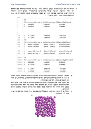
the program). It contains the positions and velocities of N=216 particles as a functions of
time, for the equilibrium system.

99
‫דו‬"‫מכין‬ ‫ח‬
2.‫מודל‬Jones-Lenard
‫א‬.‫הסב‬‫ירו‬‫בקצרה‬‫אילו‬‫עקרונות‬‫פיזיקאליים‬‫באים‬‫לידי‬‫ביטוי‬‫בפוטנציאל‬Lenard-Jones.
‫ב‬.‫מה‬‫המשמעות‬‫הפיזיקאלית‬‫וטווח‬‫הערכים‬‫הסביר‬‫של‬‫כל‬‫אחד‬‫מה‬‫פרמטרים‬‫המופיעים‬
‫בפוטנציאל‬Lenard-Jones.
‫ג‬.‫מתי‬‫הפוטנציאלית‬ ‫האנרגיה‬‫שלילית‬‫ומתי‬‫חיובית‬?‫ל‬ ‫שווה‬ ‫היא‬ ‫מתי‬‫אפס‬?‫מה‬
‫הפיזיק‬ ‫המשמעויות‬‫א‬‫ליות‬?
‫ד‬.‫קינטית‬ ‫אנרגיה‬ ‫גם‬ ‫יש‬ ‫שלמערכת‬ ‫בכך‬ ‫בהתחשב‬(‫חיובית‬),‫ל‬ ‫תצפו‬ ‫האם‬‫כוללת‬ ‫אנרגיה‬
‫שלילית‬ ‫או‬ ‫חיובית‬?‫נמקו‬.
1.‫מהן‬‫ה‬ ‫היחידות‬‫מצומצמות‬‫זה‬ ‫בשבוע‬ ‫הביצוע‬ ‫בחלק‬ ‫שימוש‬ ‫תעשו‬ ‫בהן‬?‫הנרמול‬ ‫יקבע‬ ‫כיצד‬?
2.‫מבנה‬‫ה‬‫תכנית‬:
‫א‬.‫תאר‬‫ו‬‫כל‬ ‫עושה‬ ‫מה‬‫יחידה‬‫התכנית‬ ‫של‬‫שניתנה‬.
‫ב‬.‫אפשר‬ ‫התכנית‬ ‫של‬ ‫חלקים‬ ‫אילו‬‫להש‬‫מיט‬‫של‬ ‫תנועה‬ ‫המתארת‬ ‫לתכנית‬ ‫אותה‬ ‫להפוך‬ ‫כדי‬
‫חיצוני‬ ‫בפוטנציאל‬ ‫אחד‬ ‫חלקיק‬‫נתון‬,U(r)?
‫ג‬.‫על‬ ‫האחראי‬ ‫התכנית‬ ‫של‬ ‫חלק‬ ‫אותו‬ ‫את‬ ‫אתרו‬‫התפלגות‬‫המהירויות‬.‫הסבירו‬‫היכן‬‫ו‬‫כיצד‬
‫התפלגות‬ ‫מוודא‬ ‫הוא‬‫האנרגיה‬ ‫של‬ ‫בולצמנית‬.
‫ד‬.‫היכן‬‫ו‬‫כיצד‬‫מטופלים‬‫השפה‬ ‫תנאי‬‫המערכ‬ ‫של‬‫ת‬?‫אילו‬‫קירובים‬‫נעשי‬‫ם‬,‫אם‬‫בכל‬‫ל‬?
‫ה‬.‫היכן‬‫ו‬‫ב‬ ‫התכנית‬ ‫מטפלת‬ ‫כיצד‬‫ההתחלה‬ ‫תנאי‬?‫מהן‬‫הדרכים‬ ‫שתי‬‫התכנית‬ ‫תומכת‬ ‫בהן‬
‫ההתחלתי‬ ‫האטומים‬ ‫מיקום‬ ‫לקביעת‬?
‫ו‬.‫ב‬ ‫מטפלת‬ ‫היא‬ ‫כיצד‬‫המסה‬ ‫מרכז‬ ‫תנועת‬‫המערכת‬ ‫של‬?
1.‫הסימולציה‬ ‫של‬ ‫הפרמטרים‬ ‫קלט‬:
‫א‬.‫גודל‬ ‫מהו‬‫מצומצמות‬ ‫ביחידות‬ ‫הזמן‬ ‫צעד‬?‫זה‬ ‫זמן‬ ‫מהו‬‫בשניות‬?
‫ב‬.‫זמן‬ ‫צעדי‬ ‫כמה‬ ‫כל‬‫נכתבים‬‫ומהירויות‬ ‫המיקומים‬(‫המסלול‬)‫הפלט‬ ‫לקובץ‬?
‫ג‬.‫מהו‬‫המסלול‬ ‫אורך‬(‫זמן‬ ‫בצעדי‬)?‫ב‬ ‫זה‬ ‫משך‬ ‫מהו‬‫שניות‬?
‫ד‬.‫מה‬‫החלקיקים‬ ‫מספר‬‫בסימולציה‬?
‫ה‬.‫מה‬‫הטמפרטורה‬‫בסימולציה‬?
2.‫והסבירו‬ ‫התכנית‬ ‫קוד‬ ‫את‬ ‫קראו‬‫של‬ ‫המבנה‬ ‫מהו‬‫הפלט‬ ‫קובץ‬(‫המסלול‬),traj.new.‫כיצד‬‫תיי‬‫ב‬‫או‬
‫שתבצ‬ ‫לתוכנית‬ ‫הפלט‬ ‫מקובץ‬ ‫הנתונים‬ ‫את‬‫חישובי‬ ‫ע‬‫עליהם‬ ‫ם‬?
9.‫המערכת‬ ‫גודל‬(‫הבאים‬ ‫הסעיפים‬ ‫על‬ ‫ענו‬‫פיסיקלי‬ ‫ביחידות‬‫ות‬‫חסרי‬ ‫במספרים‬ ‫ולא‬‫יחידות‬)
‫א‬.‫ארגון‬ ‫אטומי‬ ‫כמה‬‫את‬ ‫מרכיבים‬‫הסימולציה‬ ‫מערכת‬?‫ביניהם‬ ‫האינטראקציה‬ ‫מהי‬?
‫ב‬.‫מהו‬‫נפח‬‫המערכת‬?
‫ג‬.‫מהי‬‫צפיפות‬‫במערכ‬ ‫המסה‬‫ת‬?
2.‫תצפו‬ ‫מה‬‫פונקצית‬ ‫עבור‬ ‫מהתכנית‬ ‫לקבל‬‫המהירויות‬ ‫התפלגות‬?

92
2.‫גדלים‬ ‫חישוב‬‫מקרוסקופיים‬‫התכנית‬ ‫מפלט‬
‫א‬.‫מהן‬ ‫הסבירו‬‫קורלציה‬ ‫פונקציות‬‫ו‬ ‫זמניות‬‫קורלציה‬ ‫פונקציות‬‫מרחביות‬,‫ות‬‫נו‬‫לכל‬ ‫דוגמה‬
‫אחת‬.
‫ב‬.‫תארו‬‫בקצרה‬‫את‬‫ה‬‫המחושבים‬ ‫גדלים‬‫קורלציה‬ ‫מפונקציות‬‫בפרק‬"‫ביצוע‬‫הניסוי‬".
‫ג‬.‫תאר‬‫ו‬‫דרכים‬ ‫שתי‬‫הדיפוזיה‬ ‫מקדם‬ ‫לחישוב‬ ‫שונות‬‫ו‬‫ההתפלג‬ ‫פונקצית‬ ‫לחישוב‬ ‫דרך‬‫ות‬
‫הרדיאלית‬ ‫הזוגית‬‫התכנית‬ ‫מפלט‬.
‫ד‬.‫חישוב‬ ‫תוצאת‬ ‫האם‬‫אלו‬ ‫ים‬‫להיות‬ ‫יכולה‬‫השפה‬ ‫מתנאי‬ ‫מושפעת‬‫בתכנית‬?
‫במידה‬‫ולא‬,‫הסב‬‫י‬‫ר‬‫ו‬‫מדוע‬.‫במידה‬‫וכן‬,‫ה‬ ‫תהיה‬ ‫מה‬‫בזמן‬ ‫תלות‬‫של‬‫זו‬ ‫השפעה‬,‫בכלל‬ ‫אם‬?
(‫של‬ ‫במונחים‬ ‫הבע‬‫אופייניים‬ ‫גדלים‬‫המערכת‬ ‫של‬.)
‫ה‬.‫נומרית‬ ‫אינטגרציה‬:
(2)‫מהו‬‫רימן‬ ‫סכום‬‫השמאלי‬,‫הי‬‫ו‬ ‫מני‬‫כלל‬‫הטרפז‬?
(1)‫הטרפז‬ ‫בשיטת‬ ‫רק‬ ‫מדוע‬‫שונים‬‫והאחרון‬ ‫הראשון‬ ‫האיבר‬‫משאר‬‫האיברים‬?
(2)‫הסב‬‫י‬‫ר‬‫ו‬‫נותן‬ ‫מהשלושה‬ ‫איזה‬‫את‬‫ה‬‫קירוב‬‫ה‬‫טוב‬‫ב‬‫לאינטגרל‬ ‫יותר‬.
(1)‫שנקודות‬ ‫בהנחה‬‫השערוך‬‫מונוטוני‬ ‫שהאינטגרנד‬ ‫כך‬ ‫קרובות‬ ‫מספיק‬
‫במקטעים‬‫ש‬‫ביניהם‬,‫נותן‬ ‫לעיל‬ ‫רימן‬ ‫סכומי‬ ‫משלושת‬ ‫מי‬‫חסם‬‫עליון‬‫לאינט‬‫גרל‬
‫ו‬‫תחתון‬ ‫מי‬?(‫שונים‬ ‫מקטעים‬ ‫בין‬ ‫מונוטונית‬ ‫שהפונקציה‬ ‫להניח‬ ‫ניתן‬ ‫לא‬)
(2)‫של‬ ‫ערכיה‬ ‫את‬ ‫המייצגים‬ ‫עשרוניים‬ ‫משתנים‬ ‫של‬ ‫ממדי‬ ‫חד‬ ‫מערך‬ ‫בהינתן‬
‫פונקציה‬‫ו‬ ‫מסוים‬ ‫בתחום‬‫ל‬ ‫השווים‬ ‫קבועים‬ ‫במרווחים‬dt,‫הצ‬‫י‬‫ג‬‫ו‬‫זרימה‬ ‫תרשים‬
‫פסאודו‬ ‫או‬-‫קוד‬‫לחישוב‬‫ה‬‫אינטגרל‬‫הפונקציה‬ ‫של‬‫לפי‬t,‫באמצעות‬‫כלל‬‫הטרפז‬.
‫ו‬.‫אח‬ ‫לכל‬‫ת‬‫שת‬ ‫החישוב‬ ‫משיטות‬‫י‬‫ארתם‬‫בסעיף‬b,‫הצ‬‫י‬‫ג‬‫ו‬‫פסאודו‬ ‫או‬ ‫זרימה‬ ‫תרשים‬-‫קוד‬
‫לחישובם‬‫התכנית‬ ‫מפלט‬.
2.‫הצע‬‫חלופית‬ ‫אפשרות‬‫מצומצמות‬ ‫אנרגיה‬ ‫ליחידות‬,‫גדל‬ ‫על‬ ‫בהתבסס‬‫אופייניים‬ ‫ים‬‫הקיימים‬
‫במערכת‬.‫ההסבר‬ ‫פני‬ ‫על‬ ‫עדיפה‬ ‫היא‬ ‫האם‬‫החלופי‬?‫מדוע‬?
20.‫כיצד‬ ‫הסבר‬‫נדגמת‬‫פו‬‫בניסוי‬ ‫הרדיאלית‬ ‫הזוגית‬ ‫ההתפלגות‬ ‫נקצית‬‫דינאמי‬ ‫אור‬ ‫פיזור‬(DLS).
22.‫שעבור‬ ‫הראה‬‫קטנים‬ ‫הסטים‬‫המינימאלית‬ ‫הפוטנציאלית‬ ‫האנרגיה‬ ‫מקונפיגורציית‬,‫את‬ ‫לקרב‬ ‫ניתן‬
‫לנרד‬ ‫פוטנציאל‬-‫ג‬'‫הרמוני‬ ‫כפוטנציאל‬ ‫ונס‬.‫ה‬ ‫את‬ ‫בטאו‬‫עקמומיות‬‫לנארד‬ ‫פוטנציאל‬ ‫בור‬ ‫בתחתית‬-
‫ג‬'‫ואת‬ ‫ונס‬‫עומקו‬‫הפרמטר‬ ‫באמצעות‬‫הפוטנציאל‬ ‫פונקצית‬ ‫של‬ ‫ים‬.
‫א‬.‫ב‬ ‫רק‬ ‫רלוונטי‬ ‫זה‬ ‫קירוב‬ ‫מדוע‬‫נמוכות‬ ‫טמפרטורות‬?‫נמוכות‬ ‫להיות‬ ‫צריכות‬ ‫הן‬ ‫כמה‬ ‫עד‬
‫הפוטנציאל‬ ‫של‬ ‫לפרמטרים‬ ‫ביחס‬?‫ארגון‬ ‫עבור‬ ‫זו‬ ‫טמפרטורה‬ ‫להיות‬ ‫צריכה‬ ‫מה‬ ‫חשבו‬,
‫בחלק‬ ‫הפרמטרים‬ ‫בהינתן‬‫זה‬‫הניסוי‬ ‫של‬.
‫ב‬.‫לבי‬ ‫ארגון‬ ‫אטומי‬ ‫של‬ ‫גדול‬ ‫מספר‬ ‫סימולציית‬ ‫בין‬ ‫בהשוואה‬‫סימולצ‬ ‫ן‬‫י‬‫יחיד‬ ‫אוסילטור‬ ‫ית‬
(‫מחזוריים‬ ‫שפה‬ ‫תנאי‬ ‫הניחו‬ ‫המקרים‬ ‫בשני‬),‫חד‬ ‫תכונות‬ ‫אילו‬-‫תכונות‬ ‫ואילו‬ ‫חלקיקיות‬
‫רב‬-‫מהסימולציות‬ ‫אחת‬ ‫בכל‬ ‫לחשב‬ ‫ניתן‬ ‫חלקיקיות‬?‫היתרונות‬ ‫של‬ ‫השוואה‬ ‫ערכו‬
‫גישה‬ ‫בכל‬ ‫והחסרונות‬.
21.‫התדריך‬ ‫של‬ ‫זה‬ ‫בפרק‬ ‫טעויות‬ ‫גיליתם‬ ‫אם‬(‫ביצוע‬ ‫או‬ ‫הכנה‬),‫מנת‬ ‫על‬ ‫כאן‬ ‫פרטו‬‫בבונוס‬ ‫לזכות‬!

92
2.‫הדינאמיקה‬ ‫תכנית‬ ‫עם‬ ‫העבודה‬‫המולקולארית‬‫יכולה‬‫להיעשו‬‫ת‬‫דרכים‬ ‫מכמה‬ ‫באחת‬.‫לבחור‬ ‫תוכלו‬
‫לכם‬ ‫שנוחה‬ ‫קומבינציה‬ ‫כל‬.
‫א‬.‫ההפעלה‬ ‫מערכת‬ ‫בחירת‬‫העבודה‬ ‫וסביבת‬:
(2)‫א‬ ‫אלטרנטיבה‬':‫עריכה‬,‫תחת‬ ‫התוצאות‬ ‫ועיבוד‬ ‫הרצה‬LINUX.
(1)‫ב‬ ‫אלטרנטיבה‬':‫תחת‬ ‫והרצה‬ ‫עריכה‬LINUX,‫התוצאות‬ ‫לעיבוד‬ ‫הפלט‬ ‫ייצוא‬
‫אחרת‬ ‫עבודה‬ ‫בסביבת‬.
(2)‫אלטרנטיבה‬‫ג‬':‫תחת‬ ‫הרצה‬LINUX,‫התוצאות‬ ‫ועיבוד‬ ‫התכנית‬ ‫עריכת‬
‫אחרת‬ ‫עבודה‬ ‫בסביבת‬.
(1)‫ד‬ ‫אלטרנטיבה‬'(‫עתידית‬:)‫בסביבת‬ ‫מלאה‬ ‫לעבודה‬ ‫המקור‬ ‫קוד‬ ‫התאמת‬
‫אחרת‬ ‫עבודה‬.
‫ב‬.‫בחירת‬‫פלט‬ ‫קבצי‬ ‫פורמט‬:
(2)‫א‬ ‫אלטרנטיבה‬':‫בינאריים‬ ‫קבצים‬(‫מקור‬).
(1)‫אלט‬‫ב‬ ‫רנטיבה‬':‫יודפס‬ ‫שהפלט‬ ‫כך‬ ‫המקור‬ ‫קוד‬ ‫את‬ ‫לשנות‬ ‫ניתן‬‫לקובצי‬
‫טקסט‬.
‫ג‬.‫עיבוד‬ ‫סביבת‬‫ה‬‫תוצאות‬:
(2)‫א‬ ‫אלטרנטיבה‬':‫בתכנית‬ ‫התוצאות‬ ‫עיבוד‬C‫נפרדת‬.
(1)‫אלטרנטיבה‬‫ב‬':‫ו‬ ‫המקור‬ ‫קוד‬ ‫שינוי‬‫ב‬ ‫התוצאות‬ ‫עיבוד‬‫תוך‬‫תכנית‬‫ה‬C
‫המקורית‬.
(2)‫אלטרנטיבה‬‫ג‬':‫גרפי‬ ‫ממשק‬ ‫עם‬ ‫נתונים‬ ‫במסד‬ ‫התוצאות‬ ‫עיבוד‬(‫לדוגמ‬‫ה‬,
OfficeLibre Calc)
(1)‫אלטרנטיבה‬‫ד‬':‫גרפי‬ ‫ממשק‬ ‫ללא‬ ‫בתכנה‬ ‫התוצאות‬ ‫עיבוד‬(‫לדוגמה‬,
GNUPlot.)
1.‫יש‬ ‫זה‬ ‫בפרק‬‫ב‬ ‫להשתמש‬‫חישובים‬‫עבור‬‫המשקל‬ ‫שיווי‬ ‫מצב‬‫ב‬‫מסלול‬‫מקונפיגורציה‬ ‫שהתחיל‬
‫משקל‬ ‫בשיווי‬(‫מ‬ ‫נלקחה‬ ‫שלו‬ ‫שההתחלה‬ ‫כלומר‬traj.old‫מספיק‬ ‫ארוך‬)‫ו‬‫להציג‬‫התוצאות‬ ‫את‬
‫פיזיק‬ ‫ביחידות‬‫א‬‫ל‬‫מצומצמות‬ ‫ולא‬ ‫יות‬.
2.‫אנרגטיקה‬
‫א‬.‫את‬ ‫חשבו‬‫הקינטית‬ ‫האנרגיה‬‫אותה‬ ‫והציגו‬ ‫מהמהירויות‬‫נתונים‬ ‫כסדרת‬‫גרף‬ ‫על‬‫יחיד‬‫לצד‬
‫התכנית‬ ‫שנותנת‬ ‫הקינטית‬ ‫האנרגיה‬,‫האנרגיה‬‫ו‬ ‫הפוטנציאלית‬‫האנרגיה‬‫הכוללת‬‫של‬
‫הזמן‬ ‫של‬ ‫כפונקציה‬ ‫המערכת‬.‫אי‬ ‫כל‬ ‫הסבירו‬-‫התאמה‬,‫וישנה‬ ‫במידה‬.
‫ב‬.‫את‬ ‫הציגו‬‫אי‬-‫ה‬‫ה‬ ‫שימור‬‫יחסי‬‫ב‬‫אנרגיה‬‫הכוללת‬‫הזמן‬ ‫של‬ ‫כפונקציה‬.‫דונו‬‫ב‬‫הרגעית‬ ‫שגיאה‬
‫היחסית‬‫הממוצעת‬ ‫ובשגיאה‬ ‫באנרגיה‬‫היחסית‬‫באנרגיה‬,‫מאמבט‬ ‫המנותק‬ ‫לצבר‬ ‫והשוו‬
‫חום‬(‫לדוגמה‬,‫הקודם‬ ‫מהפרק‬ ‫ההרמוני‬ ‫האוסילטור‬.)

92
1.‫וט‬ ‫המהירויות‬ ‫התפלגות‬‫מפרטורה‬
‫א‬.‫מה‬‫תחום‬‫שנמדדו‬ ‫המהירויות‬?
‫ב‬.‫את‬ ‫שתחשב‬ ‫תכנית‬ ‫כתבו‬)v(P:‫הסיכוי‬‫מהירות‬ ‫יש‬ ‫אקראי‬ ‫באופן‬ ‫הנבחר‬ ‫שלאטום‬v.
‫המתקבלת‬ ‫הפונקציה‬ ‫את‬ ‫ציירו‬,‫היא‬ ‫אם‬ ‫בדקו‬‫מ‬‫תאימ‬‫ה‬‫לפונקציה‬‫ציפיתם‬ ‫לה‬(‫השוו‬
‫ונכונות‬ ‫דיוק‬ ‫ודווחו‬ ‫בטבלה‬)‫פיזיקאליים‬ ‫גדלים‬ ‫אילו‬ ‫והסבירו‬‫אחת‬ ‫בכל‬ ‫מתבטאים‬
‫הבאות‬ ‫מהתכונות‬:
(2)‫ביותר‬ ‫מסתבר‬ ‫ערך‬,‫ממוצע‬ ‫וערך‬ ‫חציוני‬ ‫ערך‬
(1)‫ראשון‬ ‫מומנט‬
(2)‫מומנט‬‫שני‬
(1)‫שונות‬
(2)‫תקן‬ ‫סטיית‬
(9)‫לפונקציה‬ ‫מתחת‬ ‫האינטגרל‬P(v)‫התחום‬ ‫כל‬ ‫פני‬ ‫על‬.
‫ג‬.‫את‬ ‫חשבו‬‫הטמפרטורה‬‫המערכת‬ ‫של‬ ‫האפקטיבית‬‫במסלול‬ ‫הנתונות‬ ‫המהירויות‬ ‫מתוך‬
‫הזמן‬ ‫כנגד‬ ‫אותה‬ ‫והציגו‬.
‫ד‬.‫בצעו‬‫התאמה‬‫את‬ ‫והציגו‬ ‫מנורמלת‬ ‫אנליטית‬ ‫לפונקציה‬ ‫שהוגרלו‬ ‫המהירויות‬ ‫התפלגות‬ ‫של‬
‫הפונקציה‬ ‫משוואת‬.
2.‫מק‬ ‫חישוב‬‫ארגון‬ ‫של‬ ‫העצמית‬ ‫הדיפוזיה‬ ‫דם‬
(‫כל‬ ‫רק‬ ‫לקובץ‬ ‫נכתבות‬ ‫שהקואורדינאטות‬ ‫זכרו‬1‫זמן‬ ‫צעדי‬)!
‫א‬.‫המהירות‬ ‫של‬ ‫עצמית‬ ‫קורלציה‬
(2)‫את‬ ‫וציירו‬ ‫חשבו‬‫פונקצית‬‫הקורלציה‬‫כפונקציה‬
‫של‬t.‫האטומים‬ ‫גבי‬ ‫על‬ ‫הוא‬ ‫המיצוע‬.‫כי‬ ‫יותר‬ ‫פשוטה‬ ‫שהנוסחה‬ ‫לב‬ ‫שימו‬
.
(1)‫היכ‬‫המידע‬ ‫נמצא‬ ‫ן‬‫הרלוונטי‬,‫ארוכים‬ ‫בזמנים‬ ‫או‬ ‫קצרים‬ ‫בזמנים‬?‫כיצד‬
‫היית‬‫ם‬‫משנ‬‫ים‬‫ערכ‬ ‫את‬‫ם‬‫של‬t‫ו‬/‫א‬‫ו‬dt*‫תוצאה‬ ‫לקבל‬ ‫כדי‬‫מדויקת‬‫יותר‬,‫ללא‬
‫ה‬ ‫הגדלת‬‫השקעה‬‫ה‬‫חישובית‬?‫בצע‬‫ו‬‫והר‬ ‫המוצע‬ ‫השינוי‬ ‫את‬‫יצו‬‫מחדש‬.‫בשאלות‬
‫שבהמשך‬,‫התשובות‬ ‫לחישוב‬ ‫ביותר‬ ‫הרלוונטי‬ ‫הזמנים‬ ‫בטווח‬ ‫התמקדו‬.
(2)‫המשמע‬ ‫מה‬‫ות‬‫הפיזיקאלי‬‫ת‬‫של‬‫האבסיסה‬ ‫ציר‬ ‫עם‬ ‫החיתוך‬ ‫נקודות‬?‫מה‬
‫של‬ ‫המשמעות‬‫שלילי‬ ‫ערך‬‫המהירות‬ ‫של‬ ‫העצמית‬ ‫הקורלציה‬ ‫עבור‬?(‫רמז‬:‫שימו‬
‫ל‬ ‫לב‬‫יחידות‬)
(1)‫בתוצאה‬ ‫השתמשו‬‫הנומרית‬(‫ההתאמה‬ ‫לפני‬)‫ל‬‫ח‬‫י‬‫ש‬‫ו‬‫הדיפוזיה‬ ‫מקדם‬ ‫ב‬
‫העצמית‬‫הנתונים‬ ‫בתנאים‬ ‫ארגון‬ ‫של‬.
‫ב‬.‫ההעתקה‬ ‫ריבוע‬ ‫ממוצע‬
(2)‫ה‬ ‫ריבוע‬ ‫ממוצע‬ ‫את‬ ‫חשבו‬‫העתקה‬‫כפונקציה‬
‫של‬t.
(1)‫ארוכים‬ ‫זמנים‬ ‫של‬ ‫בגבול‬ ‫ההעתקה‬ ‫ריבוע‬ ‫ממוצע‬ ‫התנהגות‬ ‫מה‬‫בסימולציה‬
‫שלכם‬?‫הסבירו‬.
(2)‫באיזה‬‫זמן‬ ‫של‬ ‫תחום‬‫המידע‬ ‫נמצא‬‫הרלוונטי‬?‫היית‬ ‫כיצד‬‫ם‬‫משנ‬‫ים‬‫ערכם‬ ‫את‬
‫של‬t‫ו‬/‫או‬dt*‫תוצאה‬ ‫לקבל‬ ‫כדי‬‫מדויקת‬‫יותר‬,‫החישובית‬ ‫ההשקעה‬ ‫הגדלת‬ ‫ללא‬?
‫בצע‬‫ו‬‫השינ‬ ‫את‬‫והר‬ ‫המוצע‬ ‫וי‬‫יצו‬‫מחדש‬.‫שבהמשך‬ ‫בשאלות‬,‫בטווח‬ ‫התמקדו‬
‫התשובות‬ ‫לחישוב‬ ‫ביותר‬ ‫הרלוונטי‬ ‫הזמנים‬.
(1)‫מ‬ ‫גם‬ ‫קבלו‬‫זו‬ ‫תוצאה‬‫את‬‫העצמית‬ ‫הדיפוזיה‬ ‫מקדם‬.
‫ג‬.‫הפרמטרים‬ ‫את‬ ‫שנו‬‫ובסימולציה‬ ‫קפילרי‬ ‫בניסוי‬ ‫בעבר‬ ‫שנבדקו‬ ‫לפרמטרים‬ ‫הסימולציה‬ ‫של‬,
‫בטבלה‬ ‫אליהם‬ ‫תוצאותיכם‬ ‫את‬ ‫והשוו‬ ‫מחדש‬ ‫הריצו‬(‫דווחו‬‫ונכונות‬ ‫דיוק‬.)

20
‫ד‬.‫ולתוצאות‬ ‫לתוצאותיכם‬ ‫והשוו‬ ‫בניסוי‬ ‫הראשון‬ ‫מהחלק‬ ‫הבאה‬ ‫ההכנה‬ ‫שאלת‬ ‫על‬ ‫ענו‬
‫בספרות‬.
(2)‫העצמית‬ ‫הדיפוזיה‬ ‫מקדם‬ ‫את‬ ‫העריכו‬(‫של‬ ‫נוזל‬ ‫בתוך‬ ‫חלקיק‬ ‫של‬ ‫דיפוזיה‬
‫חלקיקים‬ ‫אותם‬)‫אורך‬ ‫באמצעות‬‫החופשי‬ ‫המהלך‬ ‫ומשך‬ ‫הממוצע‬ ‫החופשי‬ ‫המהלך‬
‫הממוצע‬.‫צפיפות‬ ‫באמצעות‬ ‫התוצאה‬ ‫בטאו‬‫הנוזל‬,‫החלקיק‬ ‫מסת‬‫וה‬‫רדיוס‬‫שלו‬
(‫קלסי‬ ‫פעולה‬ ‫חתך‬)‫והטמפרטורה‬.
(1)‫את‬ ‫העריכו‬‫ארגון‬ ‫של‬ ‫העצמית‬ ‫הדיפוזיה‬ ‫מקדם‬‫בצפיפות‬2.221‫לסמ‬ ‫גרם‬"‫ק‬
‫וטמפרטורה‬21.1‫ו‬ ‫קלווין‬‫צפיפות‬ ‫עבור‬ ‫מהספרות‬ ‫ניסיונית‬ ‫לתוצאה‬ ‫השוו‬
‫דומות‬ ‫וטמפרטורה‬.‫ארגון‬ ‫של‬ ‫וולס‬ ‫דר‬ ‫ואן‬ ‫ברדיוס‬ ‫השתמשו‬,2.22‫א‬‫ו‬‫נגסטרם‬.
‫ה‬.‫ה‬‫לאי‬ ‫סיבות‬ ‫ציעו‬-‫לתוצאות‬ ‫ביחס‬ ‫החישובים‬ ‫בתוצאות‬ ‫דיוק‬‫הניסיוניו‬‫ת‬.
9.‫פונקצית‬‫ה‬‫התפלגות‬‫הזוגית‬‫הרדיאלית‬
‫א‬.‫הרדיאלית‬ ‫הזוגית‬ ‫ההתפלגות‬ ‫פונקצית‬,g(r),‫הינה‬‫פונקצית‬‫מיקומי‬ ‫של‬ ‫מותנית‬ ‫הסתברות‬
‫האטומים‬.‫ניתן‬‫לחשב‬‫אותה‬‫נומרית‬‫באמצעות‬‫היסטוגרמה‬‫מנורמלת‬‫כל‬ ‫מרחקי‬ ‫של‬
‫א‬ ‫מלבד‬ ‫האטומים‬‫מהם‬ ‫חד‬,‫האחד‬ ‫למיקום‬ ‫ביחס‬.‫פונקצית‬ ‫את‬ ‫חשבו‬‫ההתפלגות‬‫הזוגית‬
‫הרדיאלית‬,‫של‬ ‫כפונקציה‬r‫צורתה‬ ‫את‬ ‫ונתחו‬.
‫הדרכה‬:‫ש‬ ‫לב‬ ‫שימו‬‫השפה‬ ‫בתנאי‬ ‫להתחשב‬ ‫יש‬.‫כלומר‬,‫אטום‬ ‫כל‬ ‫עבור‬‫יש‬‫לבדוק‬‫את‬ ‫גם‬
‫ו‬ ‫דמותו‬‫אז‬‫הקרוב‬ ‫את‬ ‫רק‬ ‫בחישוב‬ ‫לכלול‬‫הייחוס‬ ‫אטום‬ ‫אל‬‫אלה‬ ‫שני‬ ‫מבין‬.‫זאת‬ ‫בדקו‬
‫ממד‬ ‫כל‬ ‫עבור‬(x,y,z)‫לחוד‬.
‫ב‬.‫מה‬‫מתקבל‬‫ב‬‫וגדולים‬ ‫קצרים‬ ‫מרחקים‬ ‫גבולות‬(‫כלומר‬,‫ערכים‬‫ו‬ ‫קטנים‬‫של‬ ‫גדולים‬r/σ)?
‫ג‬.‫הפרמטרים‬ ‫את‬ ‫שנו‬‫מארגון‬ ‫רנטגן‬ ‫קרני‬ ‫פיזור‬ ‫בניסוי‬ ‫בעבר‬ ‫שנבדקו‬ ‫לאלו‬ ‫הסימולציה‬ ‫של‬
‫ו‬ ‫נוזלי‬‫בטבלה‬ ‫אליהם‬ ‫תוצאותיכם‬ ‫את‬ ‫השוו‬(‫ונכונות‬ ‫דיוק‬ ‫דווחו‬.)
‫ד‬.‫לאי‬ ‫סיבות‬ ‫הציעו‬-‫בתוצאות‬ ‫דיוק‬‫הניסיוניות‬ ‫לתוצאות‬ ‫ביחס‬ ‫החישובים‬.
‫תרגיל‬‫י‬‫בונוס‬
2.‫איינשטיין‬ ‫קשר‬ ‫בהינתן‬,,‫חשב‬‫ו‬‫את‬‫החיכוך‬ ‫מקדם‬‫בנוזל‬()‫הדיפוזיה‬ ‫ממקדם‬(D.)
2.‫בדקו‬‫בזמן‬ ‫סימטריה‬‫התנועה‬ ‫משוואות‬ ‫פתרון‬ ‫של‬,‫ב‬‫השיטות‬ ‫אחת‬‫שיישמתם‬‫ב‬ ‫בחלק‬'‫הניסוי‬ ‫של‬.
2.‫וצמיגות‬ ‫לחץ‬–‫ל‬ ‫התגובה‬‫מאמצי‬‫וגזיר‬ ‫דחיסה‬‫ה‬:
‫א‬.‫הסימולציה‬ ‫מתוצאות‬ ‫בנוזל‬ ‫הלחץ‬ ‫את‬ ‫חשבו‬:‫הלחץ‬(‫האיזוטרופי‬)‫של‬ ‫התגובה‬ ‫הוא‬
‫בכיוון‬ ‫דחיסה‬ ‫למאמץ‬ ‫המערכת‬‫מסוים‬(‫נתון‬ ‫בכיוון‬ ‫מופעל‬ ‫כוח‬,‫ונעים‬ ‫מגיבים‬ ‫והאטומים‬
‫כיוון‬ ‫באותו‬.)
‫ניתן‬‫הלחץ‬ ‫את‬ ‫לחשב‬‫האינרציה‬ ‫ממומנט‬(‫היא‬ ‫בזמן‬ ‫שנגזרתו‬‫הויריאל‬):
‫ב‬.‫מתוצא‬ ‫הנוזל‬ ‫צמיגות‬ ‫את‬ ‫חשבו‬‫הסימולציה‬ ‫ות‬:‫הצמיגות‬‫ה‬‫י‬‫הנוזל‬ ‫של‬ ‫תגובה‬ ‫א‬‫ל‬‫מאמץ‬
‫גזירה‬(‫כו‬‫ח‬‫ל‬ ‫ניצב‬ ‫בכיוון‬ ‫לנוע‬ ‫לחלקיקים‬ ‫גורם‬ ‫מסוים‬ ‫בכיוון‬ ‫הנוזל‬ ‫על‬ ‫המופעל‬‫ו‬).
‫בין‬ ‫מהקורלציה‬ ‫הנוזל‬ ‫צמיגות‬ ‫את‬ ‫לחשב‬ ‫ניתן‬‫האנאיזוטרופי‬ ‫הלחץ‬:
ii.i.
iv.iii.
‫ג‬.‫בה‬ ‫מערכת‬ ‫בהינתן‬,‫להגי‬ ‫תוכל‬ ‫מה‬‫ה‬ ‫לגבי‬ ‫ד‬‫אנאיזוטרופיות‬‫של‬
‫המערכת‬?‫יהיה‬ ‫מה‬,‫לדעתך‬,‫המרחבי‬ ‫המבנה‬‫המערכת‬ ‫של‬?

22
20.‫קורלטור‬,‫קו‬‫וקו‬ ‫רלציה‬‫נבולוציה‬:
‫האוטו‬ ‫את‬ ‫נגדיר‬ ‫אם‬-‫הפונקציה‬ ‫של‬ ‫קורלטור‬fi,
‫האוטו‬ ‫את‬ ‫לבטא‬ ‫נוכל‬-‫קורלציה‬(‫העצמית‬ ‫המשותפת‬ ‫השונות‬ ‫בעצם‬,auto-covariance,‫מכיוון‬
‫שאין‬‫נרמול‬‫של‬ ‫השונות‬ ‫לפי‬f),
         
1
1
0 0,i i
N
N
i
t t t G t
N
 

    ff ff f ff f
‫השונות‬‫הצולבת‬‫העצמית‬(auto- cross-variance),
       *
0 0
0 0
*
1
1
lim lim ,
f f
i if f
t t t tN
t t t t
it tN
C t t d G t d
N
     
 
   

     ff f f
f f
‫והקונבולוציה‬(‫שבו‬ ‫שבמקרה‬f‫האוטו‬ ‫של‬ ‫הראי‬ ‫לתמונת‬ ‫שווה‬ ‫ממשית‬-‫הצולבת‬ ‫קורלציה‬),
         
0 0
0 0
1
1
lim lim ,
f f
i i
f f
t t t tN
t t t t
it tN
g t t d G t d C t
N
     
 
   

       ff f f fff f
‫הפונקציה‬ ‫ערך‬ ‫את‬ ‫לשמור‬ ‫יש‬ ‫הקורלציה‬ ‫את‬ ‫לחשב‬ ‫בכדי‬f‫בז‬‫אפס‬ ‫מן‬,‫עם‬ ‫רק‬ ‫לעבוד‬ ‫מכן‬ ‫ולאחר‬
‫בזמן‬ ‫הפונקציה‬ ‫ערך‬t‫הנוכחי‬,‫בפרק‬ ‫עתה‬ ‫זה‬ ‫שעשינו‬ ‫כפי‬‫ג‬'.‫זאת‬ ‫לעומת‬,‫את‬ ‫לחשב‬ ‫בכדי‬
‫הקונבולוציה‬,‫את‬ ‫לשמור‬ ‫יש‬‫הפונקציה‬ ‫ערכי‬ ‫כל‬f‫הזמנים‬ ‫בכל‬,t,‫בפרק‬ ‫שעשינו‬ ‫כפי‬‫א‬'.
‫בקובץ‬ ‫או‬ ‫במערך‬ ‫זאת‬ ‫לעשות‬ ‫ניתן‬,‫המערכת‬ ‫על‬ ‫מכביד‬ ‫הדבר‬ ‫מקרה‬ ‫בכל‬,‫בהיבט‬‫הזיכרון‬ ‫דרישות‬
‫החישוב‬ ‫וזמן‬ ‫הקשיח‬ ‫הזיכרון‬ ‫או‬ ‫הפנימי‬,‫בהתאמה‬.
‫א‬.‫במהירויות‬ ‫העצמית‬ ‫מהקורלציה‬ ‫הדיפוזיה‬ ‫מקדם‬ ‫את‬ ‫נוספת‬ ‫פעם‬ ‫חשבו‬,‫הפעם‬ ‫אך‬
‫ב‬‫הקונבולוציה‬ ‫בחישוב‬ ‫הקורלציה‬ ‫חישוב‬ ‫החלפת‬.‫ונכונות‬ ‫דיוק‬ ‫דווחו‬.
‫ב‬.‫א‬ ‫בפרק‬'‫תהליך‬ ‫שעבור‬ ‫ראיתם‬‫סטציונארי‬‫הקונבולוציה‬ ‫בין‬ ‫הבדל‬ ‫אין‬‫לשונות‬‫הצולבת‬.
‫כעת‬ ‫הנדון‬ ‫במקרה‬ ‫גם‬ ‫הדבר‬ ‫שכך‬ ‫קיבלתם‬ ‫האם‬?
‫ג‬.‫הערה‬:‫פשוט‬ ‫אנליטי‬ ‫ביטוי‬ ‫אין‬‫עבור‬‫פונקצית‬‫האוטו‬-‫או‬ ‫המהירויות‬ ‫של‬ ‫קורלציה‬
‫הרדיאלית‬ ‫הזוגית‬ ‫ההתפלגות‬,‫כדורים‬ ‫של‬ ‫מערכת‬ ‫כמו‬ ‫פשוט‬ ‫מודל‬ ‫עבור‬ ‫לא‬ ‫אפילו‬
‫קשיחים‬.‫ביטויים‬ ‫ישנם‬‫אינטגראליי‬‫ם‬‫בצורתם‬ ‫פשוטים‬,‫ביט‬ ‫אינם‬ ‫הם‬ ‫אך‬‫סגורים‬ ‫ויים‬.
‫כלומר‬,‫האינטגרל‬ ‫תוצאת‬ ‫עבור‬ ‫פשוט‬ ‫ביטוי‬ ‫אין‬.‫ידי‬ ‫על‬ ‫בתחום‬ ‫נעשתה‬ ‫עבודה‬‫פרופ‬'
‫ביקסון‬.

21
22.‫כקובץ‬ ‫הקונפיגורציות‬ ‫כל‬ ‫את‬ ‫הדפיסו‬‫בפורמט‬*.XYZ,‫לאפשר‬ ‫מנת‬ ‫על‬‫של‬ ‫אנימציה‬‫המסלול‬.
‫מולקולארי‬ ‫בדינאמיקה‬ ‫ביותר‬ ‫הנפוצות‬ ‫הבדיקות‬ ‫אחת‬ ‫זוהי‬‫ת‬‫מכיוו‬‫ויזואלית‬ ‫שהיא‬ ‫ן‬
‫ו‬‫אינטו‬‫איטיבית‬.‫ב‬‫ב‬ ‫אנימציה‬‫פורמט‬XYZ‫תוכנות‬ ‫באמצעות‬ ‫לצפות‬ ‫ניתן‬(‫חינמיות‬)‫כגו‬‫ן‬Jmol,
Avogadro,‫או‬VMD.‫ירא‬ ‫הקובץ‬‫ה‬,‫לדוגמ‬‫ה‬,‫כ‬‫ך‬:
Line
1 216
2 This is a comment line (can be blank): Argon cluster (216 atoms big) frame 1
3 A 0.000000 0.000000 0.000000
4 A 0.000000 0.000000 1.089000
 .
 .
 .
218 A -0.513360 -0.889165 -0.363000
219 A -0.513360 -0.889165 -0.363000
220 216
221 This is a comment line (can be blank): Argon cluster (216 atoms big) frame i
222 A x(atom 1, frame i) y(atom 1,frame i) z(atom 1, frame i)
223 A x(atom 2, frame i) y(atom 2, frame i) z(atom 2,frame i)
 …
438 A x(atom N-1, frame i) y(atom N-1, frame i) z(atom N-1, frame i)
439 A x(atom N, frame i) y(atom N, frame i) z(atom N, frame i)
 …
348582 216
348583 This is a comment line (can be blank): Argon cluster (216 atoms big) frame 1600
348584 A 0.010000 0.000000 0.000000
348584 A -0.010000 0.000000 1.089000
 …
348796 A -0.523360 -0.889165 -0.363000
348797 A -0.503360 0.889165 -0.363000
‫א‬.‫האות‬A‫את‬ ‫מייצגת‬ ‫שורה‬ ‫בכל‬ ‫הראשונה‬ ‫בעמודה‬"‫סוג‬"‫האטום‬(‫לדוגמה‬,‫היסוד‬.)‫מכיוון‬
‫ש‬Jmol‫במולקולה‬ ‫להשתתף‬ ‫שיכולים‬ ‫כאטומים‬ ‫האצילים‬ ‫ביסודות‬ ‫תומכת‬ ‫לא‬,‫לסמן‬ ‫יש‬
‫באות‬ ‫האטומים‬ ‫את‬A‫אחר‬ ‫אטום‬ ‫המייצגת‬.
‫ב‬.‫האטומים‬ ‫אחד‬ ‫אחרי‬ ‫לעקוב‬ ‫כדי‬,‫מ‬ ‫השונה‬ ‫באות‬ ‫אותו‬ ‫סמנו‬A(‫ו‬ ‫אטום‬ ‫אותו‬ ‫עבור‬‫בכל‬
‫ה‬ ‫בקובץ‬ ‫הקונפיגורציות‬*.XYZ.)‫כך‬,‫אחר‬ ‫יסוד‬ ‫של‬ ‫כאטום‬ ‫יזוהה‬ ‫האטום‬(‫ייצבע‬ ‫ולכן‬
‫אחר‬ ‫בצבע‬.)‫האטום‬ ‫שמבצע‬ ‫האקראי‬ ‫במהלך‬ ‫וצפו‬ ‫נוספת‬ ‫פעם‬ ‫האנימציה‬ ‫את‬ ‫הריצו‬
‫שבחרתם‬.
‫ג‬.‫כקובץ‬ ‫האנימציה‬ ‫את‬ ‫לייצא‬ ‫גם‬ ‫תוכלו‬(‫בפורמט‬ ‫לדוגמה‬*.gif.)‫זאת‬ ‫ועשיתם‬ ‫במידה‬,‫צרפו‬
‫לדו‬ ‫אותו‬"‫המסכם‬ ‫ח‬.

Molecular Dynamics Computer Experiment (Hebrew)

More Related Content

Similar to Molecular Dynamics Computer Experiment (Hebrew)

More from Inon Sharony

Molecular Dynamics Computer Experiment (Hebrew)