Downloaded 17 times


![Modelling Guide for Timber Structures
Structural behaviour and modelling emphases of timber, steel, and concrete structures - Chapter 2
1
2.1 INTRODUCTION
Every structural material has unique mechanical characteristics. Correspondingly, different design strategies
have been adopted for structural systems using different materials to optimise the material use. The
structural behaviour and modelling emphases of structural systems with different materials vary accordingly.
Currently, most practising engineers and researchers are more familiar with steel and concrete structures
than with timber structures, especially mass timber structures. As such, to help these practitioners become
acquainted with timber structures, this chapter compares timber structural systems with analogous ones
from steel and concrete,in terms of their structural behaviour and modelling emphases.
2.2 GENERAL COMPARISONS
2.2.1 MaterialBehaviour
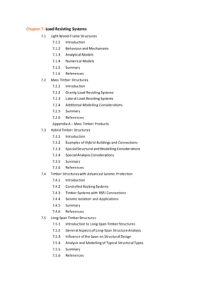
Steel (Figure 1[a]) is an iron alloy with a controlled level of carbon. It is generally considered to be a
homogeneous, isotropic, elastoplastic material with equal strength in tension and compression. It is also a
ductile material, which behaves elastically until it reaches yield, at which point it becomes plastic, and fails in
a ductile manner with large strains before fracture.
(a) (b)
Figure 1. Typical(a)steelelementsand (b)reinforced concrete
Concrete is a mixture of water, cement, and aggregates. The proportion of these components is important to
create a concrete mix of a desired compressive strength. When reinforcing steel bars are added into concrete
in bending, such as the panels shown in Figure 1(b), the two materials work together, with concrete providing
the compressive strength, and steel providing the tensile strength primarily. Conventional (plain,
unreinforced) concrete is a nonlinear, nonelastic, and generally brittle material. It is strong in compression
and weak in tension. Due to its weakness in tension capacity, concrete fails suddenly and in a brittle manner
under flexural (bending) or tensile force unless adequately reinforced with steel (Maekawa et al., 2008).
Reinforced concrete (RC) is concrete into which steel reinforcement bars, plates, or fibres have been
incorporated to strengthen a material that would otherwise be brittle.
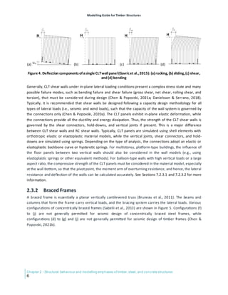
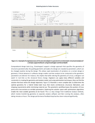
Wood (Figure 2) has characteristic anisotropy due to its fibrous structure, which can be considered as
producing three-dimensional orthotropy (Hirai, 2005). Its stiffness and strength properties vary as a function
of grain orientation among the longitudinal, radial, and tangential directions (Chen et al., 2020; Chen et al.,
2011; Sandhaas et al., 2012). The failure modes and the stress-strain relationships of wood depend on the](https://image.slidesharecdn.com/modellingguidefortimberstructures-240325073901-2a07d971/85/Modelling-Guide-for-Timber-Structures-FPInnovations-20-320.jpg)
![Modelling Guide for Timber Structures
Chapter 2 - Structural behaviour and modelling emphases of timber, steel, and concrete structures
2
direction of the load relative to the grain and on the type of load (tension, compression, or shear). For wood
in tension and shear, the stress-strain relationship is typically linear, and the failure is brittle, while for wood
in compression, the stress-strain relationship is typically nonlinear, and the failure is ductile (Forest Products
Laboratory, 2010). When loaded in tension and shear, wood elements behave in a brittle manner. On the
other hand, in compression parallel and perpendicular to the grain, wood elements show a degree of inelastic
behaviour and ductility, except under buckling, when wood is very brittle. When loaded in bending, the
ductility in wood elements is generally related to plasticisation in the compression zone, as the tension zone
tends to fail in a brittle manner. Therefore, ductility in bending is difficult to achieve in practice, and it is
recorded in tests only when the strength of the tension area is considerably higher than that of the
compression area. Similarly, shear failure of wood elements, which can happen in short, tapered beams, in
beams with end splits, or where there is stress concentration (e.g., close to notches or around holes), is
brittle, characterised by a sliding of the fibresand thus crackingparallel to the grain.
Figure 2. Threemain axesofwood withrespect tograin direction:longitudinal(L),radial(R),and tangential(T)
(Mokdad & Missoum,2013)
2.2.2 StructuralBehaviour
Due to their high strength-to-weight ratio, steel elements are, in general, relatively slender (Figure 1[a]).
Under tension, steel elements can provide excellent stiffness, strength, and ductility. However, two main
areas that require attention in the design of steel structures are buckling and connections. In compression
and bending, stability (global or local buckling) is often a concern, so the design should account for the
buckling resistance of slender steel compression and bending elements. Connections can also be a point of
relative weakness in steel structures. As such, care is needed to ensure that connections do not unduly
influence the overall response of a steel structure, especially for seismic design, where ductility is of primary
importance. In other words, connections that are not intended to yield should be capacity-protected, while
connections that are intended to yield should be designed to ensure that yielding does not progress to failure
under repeated cyclesof seismic loading.
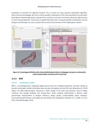
Detailing of reinforcement, particularly for seismic conditions, is a key design aspect for RC structures. As a
composite material, RC (Figure 1[b]) resists not only compression but also bending and other direct tensile
actions. The reinforcement in an RC structure, such as a steel bar, must be able to undergo the same strain or
deformation as the surrounding concrete to prevent discontinuity, slip, or separation of the two materials
under load. Maintaining composite action requires the transfer of load between the concrete and steel. The
direct stress is transferred from the concrete to the bar at the interface to change the tensile stress in the](https://image.slidesharecdn.com/modellingguidefortimberstructures-240325073901-2a07d971/85/Modelling-Guide-for-Timber-Structures-FPInnovations-21-320.jpg)

![Modelling Guide for Timber Structures
Chapter 2 - Structural behaviour and modelling emphases of timber, steel, and concrete structures
4
Timber elements generally can be simulated using orthotropic elastic material models. In some cases, such as
balloon-type mass timber walls, elastoplastic behaviour of timber elements must be included in the material
models at the wall bottom that connects to the foundation. Compared to other connections, timber
connections are much more complex due to the highly variable anisotropic mechanical properties of wood,
existing growth characteristics such as splits and knots, and other effects, such as moisture content and
temperature. Various types of failure modes can occur in timber connections, and they should have ductile
failure modes, such as yielding, rather than brittle modes, such as splitting. Where possible, the yielding
should happen in the parts of a connection that are made from a material other than wood, such as steel.
Reale et al. (2020) recommend that (a) connections with steel fasteners yielding in Johansen plastic hinge
mode that are very ductile be essential for seismic design; (b) connections with timber crushing locally that
possess limited ductility not be permitted in seismic design; and (c) connections with brittle failure, such as
splitting, not be acceptable in any cases, since the connections have effectively failed, and the load-carrying
capacity has lost once the brittle failure occurs. When properly designed, timber connections can be
simulated using models that represent the connection stiffness and strength. For analysing timber systems
under cyclic loading, suitable hysteretic models are required to accurately reflect the structural response of
timber connections and assemblies, as these may possess highly pinched hysteresis and degradation of
strength and stiffness.
In summary, the design and modelling of timber structural elements, connections, assemblies, and systems
differ from that of steel and concrete in ways that are important and usually more complex.
2.3 COMPARISONS OF SELECTEDLATERAL LOAD-RESISTING SYSTEMS
2.3.1 ShearWalls
Shear walls of cross-laminated timber (CLT) (Karacabeyli & Gagnon, 2019) are the latest lateral load-resisting
system of timber structures accepted by codes and standards around the world, such as the Engineering
design in wood standard (CSA, 2019) and the National Design Specification for Wood Construction standards
(American Wood Council, 2018), while RC shear walls are a system made of other materials that is most
similar to CLT shear walls. Both types of shear walls may take the form of isolated planar walls, flanged walls,
and larger three-dimensional assemblies such as building cores.
The structural behaviour of RC shear walls is often categorised as slender (flexure-governed) or squat (shear-
governed), according to the governing mode of damage and failure (Figure 3). Slender RC shear walls detailed
to current seismic design requirements, having low axial stress and designed with sufficient shear strength to
avoid shear failure, perform similarly to RC beam-columns. Ductile flexural behaviour with stable hysteresis
can develop up to hinge rotation limits that are a function of axial load and shear in the hinge region. Simple
slender walls (including coupled walls) can be modelled with reasonable accuracy and computational
efficiency as vertical beam-column elements with lumped flexural plastic hinges at the ends. The modelling
parameters and plastic rotation limits of the Seismic Evaluation and Retrofit of Existing Buildings standard
(American Society of Civil Engineers [ASCE], 2017) may be used for guidance. Fibre-type models are
commonly used to model slender walls, in which the wall cross-section is discretised into a number of
concrete and steel fibres. With appropriate material nonlinear axial stress-strain characteristics, the fibre wall
models can capture with reasonable accuracy the variation of axial and flexural stiffness due to concrete](https://image.slidesharecdn.com/modellingguidefortimberstructures-240325073901-2a07d971/85/Modelling-Guide-for-Timber-Structures-FPInnovations-23-320.jpg)


![Modelling Guide for Timber Structures
Chapter 2 - Structural behaviour and modelling emphases of timber, steel, and concrete structures
8
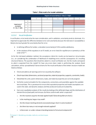
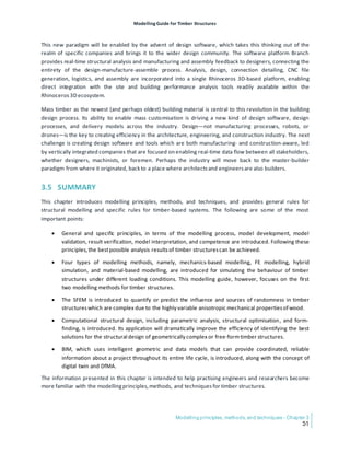
(a) (b)
Figure 6. Cyclictestingofasteelbrace (Felletal.,2010): (a)experimentalset-up,and (b) measured axial
force-deformation response
Unlike braced steel frames, braced timber frames are expected to yield and dissipate energy primarily
through energy-dissipative connections at the ends of the diagonal braces (Chen & Popovski, 2020b, 2021b).
Therefore, for braced timber frames with energy-dissipative connections, the end connections of diagonal
braces must be specially designed to sustain plastic deformation and dissipate hysteretic energy in a stable
manner through successive cycles. The design strategy is to ensure that plastic deformation occurs only in the
energy-dissipative connections, leaving the columns, braces, and beams undamaged, thus allowing the
structure to survive earthquakes without losing its gravity-load resistance. To model the behaviour of the
diagonal brace assemblies, each including a diagonal brace with two end connections (Figure 7[a]), an
equivalent nonlinear connector (spring) element can be used to simulate the total performance of the whole
diagonal brace assembly (Figure 7[b]). A continuous-column model, in which the columns are modelled using
beam elements continuously from the top to the bottom, should be ensured through design and adopted for
modelling braced timber frames (Chen et al., 2019). This can prevent underestimating the stiffness,
frequency, strength, and ductility of braced frame buildings (Bruneau et al., 2011; MacRae, 2010; MacRae et
al., 2004; Wada et al., 2009), which would occur in a pinned connection model, where the columns are
modelled using truss elements. The horizontal beams can be modelled using truss elements and pinned to
the columns, which are also connected to the ground using pin connections. See Section 7.2.3.3 for more
information.](https://image.slidesharecdn.com/modellingguidefortimberstructures-240325073901-2a07d971/85/Modelling-Guide-for-Timber-Structures-FPInnovations-27-320.jpg)
![Modelling Guide for Timber Structures
Structural behaviour and modelling emphases of timber, steel, and concrete structures - Chapter 2
9
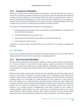
(a) (b)
Figure 7. Testingofaglued laminated (glulam)brace with riveted connections(Popovski,2004): (a)experimental
set-up,and (b)measuredaxialforce-deformation
2.3.3 Moment-Resisting Frames
Moment-resisting frames, which can be constructed using timber, steel, and concrete, are rectilinear
assemblages of beams and columns, with the beams rigidly connected to the columns. The lateral load
resistance is provided primarily by rigid frame action—that is, by the development of bending moment and
shear force in the frame elements and joints. By virtue of the rigid beam-column connections, a moment
frame cannot displace laterally without bending the beams or columns. The bending rigidity and strength of
the frame elementsis therefore the primary source of lateral stiffness and strength for the entire frame.
For non-timber systems that use capacity design principles, such as special concrete and steel moment
frames (Hamburger et al., 2016; Moehle & Hooper, 2016), the inelastic deformation should occur primarily in
flexural hinges in the beams and the column bases. In frames that do not meet special moment-frame
requirements, inelastic effects may occur in other locations, including element shear yielding, connection
failure, and element instability due to local or lateral-torsional buckling. Beam-columns are commonly
modelled using either concentrated hinges, fibre-type elements, or layered elements (Guner & Vecchio,
2010a, 2010b, 2011, 2012). Whatever the model type, the analysis should be capable of reproducing (under
cyclic loading) the element cyclic envelope curves that are similar to those from tests or other published
criteria, such as in the Seismic Evaluation and Retrofit of Existing Buildings standard (ASCE, 2017) and
Modelling and Acceptance Criteria for Seismic Design and Analysis of Tall Buildings (Applied Technology
Council, 2010). The inelastic response of flexural beams and columns is often linked to the response of the
connections and the joint panels between them. The inelastic behaviour in the beams, columns, connections,
and panel zone (Figure 8[a]) can be modelled through idealised springs, as shown in Figure 8(b). Alternatively,
it can be modelled through properly defined continuum behaviour (in equivalent fibre/layer models), along
with appropriate consideration of a finite-size panel and how its deformation affects the connected
elements. In steel structures, the yielding regions (i.e., beams, panel zones, and possibly columns and](https://image.slidesharecdn.com/modellingguidefortimberstructures-240325073901-2a07d971/85/Modelling-Guide-for-Timber-Structures-FPInnovations-28-320.jpg)


![Modelling Guide for Timber Structures
Structural behaviour and modelling emphases of timber, steel, and concrete structures - Chapter 2
13
Chen, Z., Zhu, E., & Pan, J. (2011). Numerical simulation of wood mechanical properties under complex state
of stress. Chinese Journal of Computational Mechanics, 28(4),629-634,640.
Chui, Y. H., & Ni, C. (1995, June 5–7). Dynamic response of timber frames with semi-rigid moment connections
[Conference presentation].Canadian Conference on Earthquake Engineering,Montreal, Canada.
Cortés-Puentes, W. L., & Palermo, D. (2020). Modeling of concrete shear walls retrofitted with SMA tension
braces. Journal of Earthquake Engineering, 24(4), 555-578.
https://doi.org/10.1080/13632469.2018.1452804
CSA Group.(2019).Engineering design in wood (CSA O86:19).
Danielsson, H., & Serrano, E. (2018). Cross laminated timber at in-plane beam loading – Prediction of shear
stresses in crossing areas. Engineering Structures, 171, 921-927.
https://doi.org/10.1016/j.engstruct.2018.03.018
Deierlein, G. G., Reinhorn, A. M., & Willford, M. R. (2010). NEHRP Seismic Design Technical Brief No. 4 –
Nonlinear structural analysis for seismic design: A guide for practicing engineers (NIST GCR 10-917-5).
National Institute of Standards and Technology.
European Committee for Standardization. (2004). Eurocode 5: Design of timber structures - Part 1-1: General -
Common rules and rules for buildings (EN 1995-1-1:2004).
Fell, B., Kanvinde, A. M., & Deierlein, G. G. (2010). Large-scale testing and simulation of earthquake induced
ultra low cycle fatigue in bracing members subjected to cyclic inelastic buckling (Technical Report No.
172).http://purl.stanford.edu/ry357sg5506
Fokkens, T. J. H. (2017). Behaviour timber moment connections with dowel-type fasteners reinforced with self-
tapping screws in seismic areas (Document No. A-2017.188). [Master’s thesis, Eindhoven University
of Technology].
Forest Products Laboratory. (2010). Wood handbook: Wood as an engineering material (General Technical
ReportFPL-GTR-190). U.S. Department of Agriculture.
Gavric, I., Fragiacomo, M., & Ceccotti, A. (2015). Cyclic behavior of CLT wall systems: Experimental tests and
analytical prediction models. Journal of Structural Engineering, 141(11), 4015034.
https://doi.org/10.1061/(ASCE)ST.1943-541X.0001246
Guner, S., & Vecchio, F. J. (2010a). Pushover analysis of shear-critical frames: Formulation. ACI Structural
Journal, 107(1),63-71.https://doi.org/10.14359/51663389
Guner, S., & Vecchio, F. J. (2010b). Pushover analysis of shear-critical frames: Verification and application. ACI
Structural Journal, 107(1),72-81.https://doi.org/10.14359/51663390
Guner, S., & Vecchio, F. J. (2011). Analysis of shear-critical reinforced concrete plane frame elements under
cyclic Loading. Journal of Structural Engineering, 137(8), 834-843.
https://doi.org/10.1061/(ASCE)ST.1943-541X.0000346
Guner, S., & Vecchio, F. J. (2012). Simplified method for nonlinear dynamic analysis of shear-critical frames.
ACI Structural Journal, 109(5),727-738.https://doi.org/10.14359/51684050
Hamburger, R. O., Krawinkler, H., Malley, J. O., & Adan, S. M. (2016). NEHRP Seismic Design Technical Brief
No. 2 – Seismic design of steel special moment frames: A guide for practicing engineers (NIST GCR 16-
917-41) (2nd ed.). National Institute of Standards and Technology.
https://doi.org/10.6028/NIST.GCR.16-917-41
Hirai, T. (2005). Anisotropy of wood and wood-based materials and rational structural design of timber
constructions. Proceedings of Design & Systems Conference, 15, 19-22.
https://doi.org/10.1299/jsmedsd.2005.15.19](https://image.slidesharecdn.com/modellingguidefortimberstructures-240325073901-2a07d971/85/Modelling-Guide-for-Timber-Structures-FPInnovations-32-320.jpg)
![Modelling Guide for Timber Structures
Chapter 2 - Structural behaviour and modelling emphases of timber, steel, and concrete structures
14
Karacabeyli,E., & Gagnon, S. (Eds.). (2019).Canadian CLTHandbook (2nd ed.) FPInnovations.
MacRae, G. A. (2010, March 3–5). The development and use of the continuous column concept [Conference
presentation]. Joint Proceeding of the 7th International Conference on Urban Earthquake
Engineeringand the 5th International Conference on Earthquake Engineering, Tokyo, Japan.
MacRae, G. A., Kimura, Y., & Roeder, C. (2004). Effect of column stiffness on braced frame seismic behavior.
Journal of Structural Engineering, 130(3), 381-391. https://doi.org/10.1061/(ASCE)0733-
9445(2004)130:3(381)
Maekawa, K., Vecchio, F., & Foster, S. (2008). Practitioners' guide to finite element modelling of reinforced
concrete structures (Bulletin No. 45).FIB International.
Moehle, J. P., & Hooper, J. D. (2016). NEHRP Seismic Design Technical Brief No. 1 – Seismic design of reinforced
concrete special moment frames: A guide for practicing engineers (NIST GCR 16-917-40) (2nd ed.).
National Institute of Standardsand Technology.https://doi.org/10.6028/NIST.GCR.16-917-40
Mokdad, F., & Missoum, S. (2013, August 4–7). A fully parameterized finite element model of a grand piano
soundboard for sensitivity analysis of the dynamic behavior [Conference presentation]. ASME 2013
International Design Engineering Technical Conferences and Computers and Information in
EngineeringConference,Portland,USA.
Negrão, J. H., Brito, L. D., Dias, A. G., Júnior, C. C., & Lahr, F. R. (2016). Numerical and experimental study of
small-scale moment-resistant reinforced concrete joints for timber frames. Construction and Building
Materials, 118,89-103.
Palermo, D., & Vecchio, F. J. (2007). Simulation of cyclically loaded concrete structures based on the finite-
element method. Journal of Structural Engineering, 133(5), 728-738.
https://doi.org/10.1061/(ASCE)0733-9445(2007)133:5(728)
Popovski, M. (2004).Structural systems with riveted connections for non-residential buildings.FPInnovations.
Reale, V., Kaminski, S., Lawrence, A., Grant, D., Fragiacomo, M., Follesa, M., & Casagrande, D. (2020). A
review of the state-of-the-art international guidelines for seismic design of timber structures
[Conference presentation].World Conference on Earthquake Engineering,Sendai, Japan.
Rinaldin, G., Amadio, C., & Fragiacomo, M. (2013). A component approach for the hysteretic behaviour of
connections in cross-laminated wooden structures. Earthquake Engineering & Structural Dynamics,
42(13),2023-2042.https://doi.org/10.1002/eqe.2310
Sabelli, R., Roeder, C. W., & Hajjar, J. F. (2013). NEHRP Seismic Design Technical Brief No. 8 – Seismic design of
steel special concentrically braced frame systems: A guide for practicing engineers (NIST GCR 13-917-
24). National Institute of Standards and Technology.
Sandhaas, C., Van de Kuilen, J.-W., & Blass, H. J. (2012, July 15–19). Constitutive model for wood based on
continuum damage mechanics [Conference presentation]. World Conference on Timber Engineering,
Auckland,New Zealand. http://resolver.tudelft.nl/uuid:55c1c5e5-9902-43ad-a724-62bb063c3c80
Schachter, M., & Reinhorn, A. M. (2007). Three-dimensional modeling of inelastic buckling in frame structures
(Technical ReportMCEER-07-0016). Multidisciplinary Center for Earthquake EngineeringResearch.
Tang, T. O., & Su, R. K. L. (2014). Shear and flexural stiffnesses of reinforced concrete shear walls subjected to
cyclic loading. The Open Construction and Building Technology Journal, 8, 104-121.
Tang, X., & Goel, S. C. (1989). Brace fractures and analysis of phase I structure. Journal of Structural
Engineering, 115(8),1960-1976.https://doi.org/10.1061/(ASCE)0733-9445(1989)115:8(1960)
Uriz, P., & Mahin, S. (2008). Towards earthquake-resistant design of concentrically braced steel-frame
structures. Pacific Earthquake EngineeringResearch Center.](https://image.slidesharecdn.com/modellingguidefortimberstructures-240325073901-2a07d971/85/Modelling-Guide-for-Timber-Structures-FPInnovations-33-320.jpg)


![Modelling Guide for Timber Structures
Modelling principles, methods, and techniques - Chapter 3
7
different solvers (e.g., explicit or implicit solvers). With Abaqus, many researchers have developed user
subroutines that can model the unique structural behaviour of wood-based components, connections,
assemblies, and even entire building structures, which are unavailable in most software packages. This has
resulted in many consultant companies using this type of software in their design practice in recent years. For
a conventional structural analysis, design-oriented software packages such as SAP2000, ETABS, S-FRAME, and
Dlubal are the best options. However, they usually have limited capacity to model certain types of structures
and have limited types of FEs compared to general-purpose programs. Their advantage is their capacity to
more easily model structures commonly found in the architecture, engineering, and construction industry
and to carry out design checks based on any codes and standards that have been preprogrammed. They can
therefore quickly post-process the analysis results and design the structure according to codes of practice.
Currently, more and more structural design programs have preliminary added wood modules, such as Dlubal,
S-FRAME, SAFI, and RISA, and some have been specifically developed for modelling, analysis, and design of
wood structures, such as S-TIMBER. These software programs provide a more user-friendly function for
practising engineersto design timber structures.
3.2.2.3 Principles of Model Development
A useful strategy in the early part of modelling is to draw up an issue or feature list to help in making
decisions about the model. The features are the factors that may need to be considered in relation to the
model, in terms of material behaviour, loading, boundary conditions, etc. The next step is to develop a
computational model incorporating the means of achieving a solution, such as the type of FE scheme to be
used and the degree of mesh refinement. In some cases where new structures are to be analysed, it may be
best not to develop just one model but to investigate a few options, evaluate them, and choose the one to be
used. The general rules for structural model development of timber structures are listed below. Specific
principlesand considerationsfor timber structuresare indicated by [√].
• Start with a simple model and refine it step by step. If you decide to move into an area of analysis
that is unfamiliar, build experience by starting with simple (smaller) elastic models and load cases for
which solutions are known, if practical. If using nonlinear analysis, start with an elastic model, then
move into separate nonlinear material and nonlinear geometry models, and then combine them. At
each stage, reviewthe resultsto assess whether they are acceptable.
• Keep the model at a level as simple as practical. More precise and complicated modelling should
focus on key structural components and connections, while simplifications can be made on parts of
the structure that are of secondary importance.
• Ensure that the modelis sufficiently detailed and realistic, but not overly complicated.
• Select a suitable type of model (1D, 2D versus 3D) based on the analysis problem and the
characteristicsof the structure.
• Use symmetry to reduce computation/analysis resource demand. If a structure has an axis of
symmetry, then the order of solution can be reduced. While the need to reduce the size of models is
now less important due to the high level of computing power available, there may be circumstances
in which the use of a symmetric model is disadvantageous, such as in frequency analysis (any
unsymmetric modes that actually exist in the full model cannot be represented). For mirror
symmetry to be satisfied, all geometric and material properties and all loading must be the same at](https://image.slidesharecdn.com/modellingguidefortimberstructures-240325073901-2a07d971/85/Modelling-Guide-for-Timber-Structures-FPInnovations-43-320.jpg)
![Modelling Guide for Timber Structures
Chapter 3 - Modelling principles, methods, and techniques
8
corresponding points on either side of the axis of symmetry. The cross-sectional properties of the
member on the axis of symmetry of the symmetrical (antisymmetric ally) equivalent model are half
of those for the complete frame.
• [√] Remember that the structural and material behaviour of timber structures is different from
that of other types of structures, such as steel or concrete, and the modelling is correspondingly
different. See Chapter 2 for more information.
• Choose appropriate elements for the structural components. Usually, there are many types of
elements to choose from. The choice is often obvious, but consider the following guidelines and pick
the onesmost suitable based on the conventional rulesand the output requirements.
o Line elements(these are for memberswith length-to-width ratios that are sufficiently high):
Bar/truss elements: Straight, with only one axial degree of freedom at each end. Such
elementsare typically used to model pin-connected struts.
Beam elements: Include (a) a plane frame (2D beam) element incorporating a single plane of
bending plus axial effects with three degrees of freedom per node; (b) a grillage element
incorporating a single plane of bending and torsional effects; and (c) 3D beam element
incorporating bending in two planes, axial and torsional actions, with six degrees of freedom
at each node. In all cases, the bending component may include shear deformation (thick
beam) or neglectshear deformation (thin beam).
o Surface elements:
Plane stress (membrane) elements: No stress and no restraint to movement in the out-of-
plane direction.
Plane strain elements: No strain, but there is stress in the out-of-plane direction.
Plane bending elements (basic components of traditional flat shell elements): To model flat
plates that are subjected only to out-of-plane bending actions. The boundary between thin
and thick plate bending theories is a span-to-depth ratio of 10:1. A small deflection
assumption is validated when the maximum deflection is less than the plate depth for thin
plates.
Shell elements: To model curved surfaces and flat plates for which in-plane and out-of-plane
actions need to be factored in. Shell elements tend to have six degrees of freedom at each
node, taking into account in-plane (membrane) and out-of-plane (bending) actions. They can
be flat or curved.
o Volume elements (3D elements, or brick elements): Tend to be used more in advanced structural
analysis and mass structuresof nonlinear and elastic soils.
• Conduct convergence analysis to assess the meshing strategies for FE models. Convergence for
mesh refinement implies that as mesh density is increased, the results will converge towards the
exact solutions. The rate of convergence depends on the type of element, the number of elements in
the mesh, and the loading type. Meshing principlesare listed below.
o FE meshing is more of an art than a science. The more we experiment with it, the better we
become.](https://image.slidesharecdn.com/modellingguidefortimberstructures-240325073901-2a07d971/85/Modelling-Guide-for-Timber-Structures-FPInnovations-44-320.jpg)
![Modelling Guide for Timber Structures
Modelling principles, methods, and techniques - Chapter 3
9
o Mesh density: A basic principle is to choose a mesh density at which the convergence curve
starts to flatten off. The challenge,of course,is that there is rarely a convergence curve.
o Quadrilateral versus triangular: Quadrilateral elements are more accurate and should always be
preferred over triangular ones. Modern meshing algorithms primarily use quadrilateral elements
and triangular ones only when absolutely necessary due to geometric constraints.
o Element shape: The ideal shape for a quadrilateral element is a square and for a triangular
element an equilateral triangle. As the shapes of these elements deviate from the ideal shapes,
so does their accuracy. Many structural analysis programs issue a warning when the element
shape is distorted to the point where its accuracy is questionable. An accurate mesh usually
looks good to the eye. If a mesh looks ugly to you, you should probably replace it with another
mesh. Automatic meshing is available in many structural analysis programs and should be used
to improve the quality of meshes.
o Curved boundaries: Typically, a larger number of elements is needed to accurately represent a
curved boundary (circular, elliptic, etc.) than a straight boundary. As a rule of thumb, some
element boundaries can be curved. Accuracy for these elements decreases as the sides’ offset
from straight increases.
o Stress gradients: A good strategy is to have a finer mesh in areas of a high stress gradient and a
coarser mesh where the stress gradient is low. However, for models with a large number of
elements it may be best to investigate stress concentrations in separate detailed models (e.g.,
using sub-modelling to study the detailed stress distribution in the area of an important
connection).
• [√] Choose appropriate material models for structural components. In structural analysis the
constitutive relationships tend to have the following two assumptions: (1) a definition of material
behaviour (e.g., linear elastic behaviour or plasticity); and (2) assumptions with regard to the stress
distribution within the differential element types. For example, for the plane stress condition,
stresses are defined in a plane with zero stress at right angles to the plane; for bending elements
(such as beams and shells), the stresses are assumed to vary linearly within the depth of the
element. Wood is an anisotropic material with a different stress-strain response in different
directions or under different loading conditions in the same directions (Chen et al., 2011, 2020). Such
complex response induces various types of failure modes in the wood components and connections.
Therefore, the material constitutive model should be chosen to meet the model requirements.
Correct material models can help predict specific yield and failure modes of wood components and
connections.See Chapter 4 for more information.
• [√] Choose appropriate elements for connections. Select pinned, rigid, or semirigid types according
to the structure you are investigating. Joint elements, which are used for modelling plastic hinges
and semirigid connections, normally consist of a set of springs that connect two nodes or two
freedoms (e.g., linear elastic spring and elastoplastic spring). The depths of beams or columns and
eccentricities need to be modelled properly. For timber structures, the connections typically play a
key role in the structural response (e.g., deformation and resistance). Therefore, it is crucial to model
the timber connections using an appropriate method (Chen & Chui, 2017; Chen et al., 2013; Reale et
al., 2020). For capacity-based design timber structures, the timber components can be simulated as
elastic material, while the energy-dissipative connections should be simulated with elastoplastic](https://image.slidesharecdn.com/modellingguidefortimberstructures-240325073901-2a07d971/85/Modelling-Guide-for-Timber-Structures-FPInnovations-45-320.jpg)
![Modelling Guide for Timber Structures
Chapter 3 - Modelling principles, methods, and techniques
10
behaviour. Also note that timber connections have high variability in stiffness and strength (Jockwer
& Jorissen, 2018).See Chapter 5 for more information.
One very important part of the detailed analyses is the design of connections. As it is extremely
complex to model the anisotropy of timber given the imperfections of the material, these analyses
should involve careful calculation that factors in all of the different failure modes (e.g., splitting and
block shearing) as defined and codified by the most up-to-date standards and guidance, such as
Eurocode 5 (European Committee for Standardization, 2004).
• [√] Choose appropriate force-deformation models for assemblies if macroelements are used.
Timber assemblies, such as shear walls, respond differently from steel and concrete assemblies (e.g.,
pinching effect); the force-deformation models should be chosen to meet the model requirements.
See Chapters 6 and 7 for more information.
• Adopt appropriate model input. The required model input varies according to the modelling
situation: (a) analysis objectives: design values are needed for practising design while test results are
preferred for research; and (b) analysis types: less input for elastic or static analyses and more for
nonlinear or dynamic analyses. The necessary parameters for the models and how they can be
derived are discussed in Chapters4 to 10.
• Choose appropriate types of constraints on the structural components and assemblies. Constraints
are conditions imposed on the deformation of a structure—effectively a compatibility condition.
Constraints can be incorporated into the model using constraint equations, a rigid link, and a beam
element.
• Choose appropriate types of loads applied to the structural components and assemblies. A point
load usually induces a stress concentration issue. Such an issue, however, can be avoided by applying
the load on a certain area. Judge whether the effect of finite widths of members at the connections
can be neglected.
• Choose appropriate types of support applied to the structural components and assemblies. An
analysis model of a structure must be defined in relation to a frame of reference. It must be fixed in
space; it must be supported. A reaction force corresponds to each restrained freedom of the
structure. These reaction forces must at least form a set that is statically determinate. Conventional
restraints include a horizontal roller, pin, fixed restraint, vertical roller (nonrotation, at axis of
symmetry), and translational and rotational springs. Neglecting fixity where there is a degree of
restraint tends to be conservative for estimates of deformation and internal forces. The assumption
that a column is fully restrained at its base may result in an overestimate of stiffness and an
underestimate of the maximum frame moments. Issues to be considered when validating a fixed
column support include (a) whether the stiffness of the frame is a critical issue; and (b) the detailing
at the support (i.e., is the foundation sufficiently massive that the rotational stiffness at the support
will be negligible?).](https://image.slidesharecdn.com/modellingguidefortimberstructures-240325073901-2a07d971/85/Modelling-Guide-for-Timber-Structures-FPInnovations-46-320.jpg)
![Modelling Guide for Timber Structures
Modelling principles, methods, and techniques - Chapter 3
11
• Choose an appropriate type of foundation model for the structure. In this context the structure
includes the superstructure and the foundation, and the ground that is below the foundation,
including soil and rock. The model of a structure is more likely to be realistic if the deformation of a
rock support is included than if the effect of a soil support is neglected. Four basic ways of defining
the supports for a structure (Figure 3) are:
o Support fixity model: Deformations of the ground are ignored and the nodes for the structure at
the contact with the ground are given fixed restraints.
o Winkler model: The ground is modelled by linear elastic springs at the structure-soil interface.
The springs are not coupled (i.e., when one spring deforms, the other springs are unaffected by
shear transfer in the ground).
o Half-space model: The ground is modelled by coupled springs at the structure-soil interface
(i.e., shear transfer in the ground is factored in).
o Element model for the ground: The ground is modelled using FEs that have fixities adequately far
away from the superstructure.
(a) (b) (c) (d)
Figure 3. Modelsfor structuresupport(MacLeod,2010): (a)supportfixitymodel,(b)Winkler spring
model,(c)half-space model,and (d)element modelofground
Soil tends to be nonhomogeneous, with mechanical properties that may be time-dependent,
functions of water content, and nonlinear in relation to stress and strain. Addressing these features
requires advanced analysis that is outside the scope of this guide. Taking account of the structure
and the ground in a single analysis is known as soil-structure interaction. This is very difficult to
model accurately. While ‘garbage in, garbage out’ needs to be avoided, using approximate models
(such as the Winkler model) is better than completely ignoring the impact foundations can have on
the behaviour of a superstructure.See Chapters7 to 10 for more information.
• [√] Develop appropriate load paths in the structure. Ensure that proper load paths have been
designed into the structure and that the models can reflect the corresponding load paths (Reale et
al., 2020). Understanding how vertical and lateral load is distributed in a structure is an essential
feature in modelling. It depends on the continuity (simply-supported versus continuous) and stiffness
(flexible versus rigid) of the member directly resisting the loads, and the stiffness (flexible versus
rigid) of the members supporting the former. The load paths are especially important for structures
with load-resisting elements/assemblies with significant stiffness (e.g., hybrid timber structures). See
Chapters 8 to 10 for more information.](https://image.slidesharecdn.com/modellingguidefortimberstructures-240325073901-2a07d971/85/Modelling-Guide-for-Timber-Structures-FPInnovations-47-320.jpg)
![Modelling Guide for Timber Structures
Chapter 3 - Modelling principles, methods, and techniques
12
• Consider nonstructural elements and non–lateral load-resisting elements according to engineering
judgment. Also carefully consider the actual stiffness and strength of all possible lateral load-
resisting structures in all directions. Secondary, facade, or nonstructural walls or structures may all
carry significant loads, and beams may provide unintended coupling action between shear walls. See
Chapters 7 to 10 for more information.
• Consider nonlinear geometry in the models, if necessary. When a structure is loaded, the geometry
changes. The change in geometry causes the relationship between loads and displacements to be
nonlinear,and hence this is described as geometric nonlinearity.
Criterion for neglecting nonlinear geometry effects: The critical load ratio (λ), the ratio between the
axial load and the elastic critical load, is the main parameter for assessing the potential effects of
nonlinear geometry. If λ is less than 0.1, then the nonlinear geometry effects can be ignored;
otherwise, they should be accounted for in the models. Apart from the level of the applied load, the
main factor affecting the nonlinear geometry effect is the stiffness of the structure. This depends on
several parameters, including the material properties, such as Young’s and shear moduli, connection
types, support conditions, restraints, and cross-sectional properties. During the sizing of members,
the minimum slender ratio should be considered as specified in the design standards. In some cases,
elastic limits may be exceeded before a critical condition is reached, and nonlinear material
behaviour must be factored in. See Chapters8 to 10 for more information.
• Consider appropriate loading conditions in the models. The term loading can imply the general
concept of external action on the structure. In this context it implies dead load, live load, snow loads,
wind loads, and seismic loads. In bridge design in particular, it is important to manipulate loads
whose position on the structure is not fixed (e.g., moving loads). The influence line is the main
technique used to identify critical positions of moving loads. The best pattern of loading must be
considered for bridges,floors, and roofs. See Chapters6 and 8 to 10 for more information.
• [√] Consider both local and resultant stresses in modelling of timber structures, if necessary. For
example, for a simply-supported beam under two-point loading, the horizontal direct stress
(i.e., compression and tension) is the resultant stress due to the bending moment, while the local
effect is compression perpendicular to the grain in the vicinity of the point loads and supports.
Unlike with steel and concrete, the compression strength perpendicular to the grain of wood-based
materials is an order of magnitude lower than the strength parallel to the grain. Therefore, whereas
the local effect can be ignored in a steel structure, it must be accounted for when modelling timber
structures.
• [√] Develop a good model based on the knowledge of the investigated members, connections, and
structures. The observance of physical behaviour is one of the most important strategies for
developing a good understanding of a structure’s behaviour, which can help in developing more
accurate models. This is especially important for timber structures.](https://image.slidesharecdn.com/modellingguidefortimberstructures-240325073901-2a07d971/85/Modelling-Guide-for-Timber-Structures-FPInnovations-48-320.jpg)

![Modelling Guide for Timber Structures
Modelling principles, methods, and techniques - Chapter 3
15
o Are there any inappropriate offsets?
o Are all loads presentor are some missing (e.g., torsion)? Are they applied correctly?
o If the structure is symmetric, then it is worth applying a symmetric loading case and checking the
corresponding deformation (or force actions) in relation to a pair of symmetric degrees of
freedom.
• Check the resultsfrom the developed numerical modelsagainst:
o Simplified methods of calculation or test results. For example, the fundamental periods of the
tall wood buildings computed by modal analysis should be compared with available empirical
formulas (Karacabeyli & Lum, 2022) and any available similar test data to ensure the results are
not biased.
o Analysis results of a checking model that is a simplified version of the main model but has
adequate accuracy for checkingpurposes.
o If a static analysis is being performed, a free vibration analysis should also be run, and vice versa.
Do the resultsmake sense?
• Check the specific timber structural models, including:
o Components: elasticity, yielding, and local failure.
o Connections: energy-dissipative and non-dissipative connections.
3.2.3.3 Sensitivity Check
A sensitivity analysis investigates the effects of different values for features or parameters. The need for a
sensitivity analysis depends on the degree of uncertainty of key model parameters (dimensions, material
properties, section properties, loads [e.g., combinations and patterns], among others). When working on an
unusual structural design, a sensitivity analysis may be essential to gain a better understanding of the general
behaviour of the model and to increase confidence in the model. The following issues are relevant to
sensitivity analysis:
• Work from a reference model, changing one variable at a time and reverting to the reference model
after each change. As the designer gains understanding, it may be better to change the reference
model, but if the changes are compounded it becomes difficult to make sensible comparisons. This
can lead to an overwhelmingly large number of permutations, and formal procedures may be
required to properly interpret the results. This topic is dealt with in the study of robust design,
design of experiments, and optimisation. Some structural analysis programs are beginning to offer
rudimentary tools to assist the designer (e.g., the multiple scenarios feature in S-FRAME, which
allows the designer to evaluate multiple modellinginstances of the same structure in a single run).
• Make comparisons with indicative parameters (i.e., parameters that tend to exemplify the
behaviour).Typical indicative parametersinclude:
o Maximum deflection in the direction of the main loading;
o Deflection in the line of a single-point load used as a checkingload case;](https://image.slidesharecdn.com/modellingguidefortimberstructures-240325073901-2a07d971/85/Modelling-Guide-for-Timber-Structures-FPInnovations-51-320.jpg)


![Modelling Guide for Timber Structures
Modelling principles, methods, and techniques - Chapter 3
45
approaches to data structures (CAD standards), and is stored in standard formats that can be exchanged
between different CAD applications. Also, level 1 replaces the ad hoc information exchange mechanisms with
the introduction of a common data environment (CDE), which is used to share and exchange CAD files
between various project participants. However, traditional CAD information still consists of drawings and
documents without any embedded intelligence, which can offer opportunities for information integration by
unlocking the potential of collaborative working. Level 2 denotes a managed BIM environment that contains
intelligent BIM models held in separate disciplines (discipline models), shared and coordinated using a
structured approach in a CDE, and integrated using proprietary or customised middleware for design (e.g.,
architectural, structural), analysis (e.g., energy analysis, clash detection), project management (e.g., 4D, 5D),
and maintenance purposes (e.g., construction operations building information exchange). Level 2 BIM is most
desired by client organisations, as it can be achieved without fundamental changes to business practices and
can provide significant improvements in project delivery. Level 3 BIM denotes fully integrated and
collaborative BIM, which is enabled by web services to facilitate collaborative building information using
open standards (e.g., industry foundation class [IFC]) without interoperability issues. It also extends the use
of BIM applications towards the life cycle management of building projects.
To achieve high-performing, low-cost built environments, BIM adoption requires a higher level of
collaborative work among construction disciplines beyond the traditional work boundaries and restricted
contractual relationships. Also, early project stages are critical for establishing comprehensive BIM
development and implementation strategies that can facilitate integration and collaboration among team
members through the entire project(Porwal & Hewage, 2013).
Various BIM software packages are provided by different companies (e.g., Autodesk, Bentley, ArchiCAD).
Using these software packages, designers from different disciplines working on a project can generate
detailed digital representations of a building or infrastructure and allow for coordination from the early
design stages. At the same time, because the objects modelled are not solely geometric but also embed
different properties, several evaluations (e.g., material quantities, energy characteristics, schedules of
elements) can be extracted from the model. In addition, BIM software packages generally allow detailed
construction drawings to be extracted directly from the model and remain up-to-date throughout the process
and capture all the changes, with limited interaction required from the drawing technicians. Figure 26
presents a typical framework of a CDE, developed by Shafiq (2019) using Bentley’s ProjectWise, which
coordinated with the BIM (architecture, structure, mechanical, electrical, and plumbing) developed using
Autodesk Revit Suite. ProjectWise is a model collaboration platform that supports native Revit model
exchanges, providing document management services with model-based project management support. The
BIM models were developed using the Autodesk Revit platform (i.e., Revit architecture; Revit mechanical,
electrical, and plumbing; and Revit structure), which used inputs from 2D documents and drawings. All the
models were exchanged using the CDE through ProjectWise. Moreover, Navisworks was used to create 4D
models (taking a feed from a Primavera P6 schedule and LOD 300 Revit model), and Autodesk BIM 360 Glue
was used for document management and cloud-enabled information for synchronisation and collaboration.
The interoperability issueswere resolved using the IFC format and the xBIM IFC viewer and analyser.](https://image.slidesharecdn.com/modellingguidefortimberstructures-240325073901-2a07d971/85/Modelling-Guide-for-Timber-Structures-FPInnovations-81-320.jpg)
![Modelling Guide for Timber Structures
Chapter 3 - Modelling principles, methods, and techniques
46
Figure 26. The structureofaproject CDE(Shafiq,2019)
All the project participants should agree to follow the implementation of the LOD as defined by a specific
protocol (e.g., the LOD specification by BIMForum [2020]). The model will be progressively developed from
LOD 100 to LOD 300 at the design stage (Table 2), which is used to generate collaborative design reviews and
clash detection, and constructability reviews. The methodology and nomenclature of the BIMForum’s LOD
specification are used to control the information sharing and collaboration tasks (i.e., work in progress,
shared, published, and archived). Further, the fully coordinated clash-free BIM model (LOD 300) is handed
over to the successful bidder at the tender stage to further develop the LOD 400 model. The LOD 400 model
is used to perform construction clash detection (e.g., clearances) and 4D simulations to support the planning
process. It is the contractor’s responsibility to update the LOD 400 model with the as-built information (floor
by floor) and submit it to the client with the required information for the facility management tasks, thus
deliveringan as-built model (LOD 500) at the projecthandover.](https://image.slidesharecdn.com/modellingguidefortimberstructures-240325073901-2a07d971/85/Modelling-Guide-for-Timber-Structures-FPInnovations-82-320.jpg)


![Modelling Guide for Timber Structures
Chapter 3 - Modelling principles, methods, and techniques
52
3.6 ACKNOWLEDGEMENTS
The authors would like to acknowledge Ms. Maja Belic for her contributionsto Section 3.4.3.
3.7 REFERENCES
Abanda, F. H., Vidalakis, C., Oti, A. H., & Tah, J. H. M. (2015). A critical analysis of building information
modelling systems used in construction projects. Advances in Engineering Software, 90, 183-201.
https://doi.org/10.1016/j.advengsoft.2015.08.009
Ariaratnam, S. T., Schuëller, G. I., & Elishakoff, I. (Eds.). (1988). Stochastic structural dynamics: Progress in
theory and applications.Elsevier Applied Science.
Arregui-Mena, J. D., Margetts, L., & Mummery, P. M. (2016). Practical application of the stochastic finite
element method. Archives of Computational Methods in Engineering, 23(1), 171-190.
https://doi.org/10.1007/s11831-014-9139-3
Astill, C. J., Imosseir, S. B., & Shinozuka, M. (1972). Impact loading on structures with random properties.
Journal of Structural Mechanics, 1(1),63-77.https://doi.org/10.1080/03601217208905333
Bew, M., & Richards, M. (2008). BIM maturity model [Paper presentation]. Construct IT Autumn 2008
Members’ Meeting, Brighton, UK.
BIMForum. (2020). Level of development (LOD) specification: Part I & commentary for building information
models and data.
Brandner, R., & Schickhofer, G. (2014). Length effects on tensile strength in timber members with and
without joints. In S. Aicher, H. W. Reinhardt, & Garrecht (Eds.), Materials and Joints in Timber
Structures (pp. 751-760). RILEM Bookseries, Vol. 9. Springer, Dordrecht.
https://doi.org/10.1007/978-94-007-7811-5_67
British Standards Institution. (2013). Specification for information management for the capital/delivery phase
of construction projects using building information modelling (PAS 1192-2:2013).
Chen, Z., & Chui, Y.-H. (2017). Lateral load-resisting system using mass timber panel for high-rise buildings.
Frontiers in Built Environment, 3(40). https://doi.org/10.3389/fbuil.2017.00040
Chen, Z., Chui, Y.-H., Doudak, G., & Nott, A. (2016). Contribution of type-x gypsum wall board to the racking
performance of light-frame wood shear walls. Journal of Structural Engineering, 142(5), 4016008.
https://doi.org/10.1061/(ASCE)ST.1943-541X.0001468
Chen, Z., Chui, Y. H., Mohammad, M., Doudak, G., & Ni, C. (2014, August 10–14). Load distribution in lateral
load resisting elements of timber structures [Conference presentation]. World Conference on Timber
Engineering,Quebec City, Canada.
Chen, Z., Chui, Y. H., Ni, C., Doudak, G., & Mohammad, M. (2014). Load distribution in timber structures
consisting of multiple lateral load resisting elements with different stiffness. Journal of Performance
of Constructed Facilities, 28(6).https://doi.org/10.1061
Chen, Z., Chui, Y. H., Ni, C., & Xu, J. (2014). Seismic response of midrise light wood-frame buildings with portal
frames. Journal of Structural Engineering, 140(8), A4013003. https://doi.org/10.1061/(ASCE)ST.1943-
541X.0000882
Chen, Z., Chui, Y. H., & Popovski, M. (2015). Development of lateral load resisting system. In Y. H. Chui (Ed.),
Application of analysis tools from NEWBuildS research network in design of a high-rise wood building
(pp. 15-36).](https://image.slidesharecdn.com/modellingguidefortimberstructures-240325073901-2a07d971/85/Modelling-Guide-for-Timber-Structures-FPInnovations-88-320.jpg)


![Modelling Guide for Timber Structures
Modelling principles, methods, and techniques - Chapter 3
55
MacLeod,I. A. (2010).Modern structural analysis: Modelling process and guidance.Thomas Telford.
Madsen, B. (1990). Size effects in defect-free Douglas fir. Canadian Journal of Civil Engineering, 17(2), 238-
242.https://doi.org/10.1139/l90-029
Madsen, B., & Tomoi, M. (1991). Size effects occurring in defect-free spruce – pine – fir bending specimens.
Canadian Journal of Civil Engineering, 18(4),637-643.https://doi.org/10.1139/l91-078
Martínez-Martínez, J. E., Alonso-Martínez, M., Álvarez Rabanal, F. P., & del Coz Díaz, J. J. (2018). Finite
element analysis of composite laminated timber (CLT). Proceedings of the 2nd International Research
Conference on Sustainable Energy, Engineering, Materials and Environment, 2(23), 1454.
https://doi.org/10.3390/proceedings2231454
Matheron, G. (1973). The intrinsic random functions and their applications. Advances in Applied Probability,
5(3), 439-468.https://doi.org/10.2307/1425829
Melchers,R. E., & Beck,A. T. (2017).Structural reliability: Analysisand prediction. Wiley.
Moens, D., & Vandepitte, D. (2006). Recent advances in non-probabilistic approaches for non-deterministic
dynamic finite element analysis. Archives of Computational Methods in Engineering, 13(3), 389-464.
https://doi.org/10.1007/BF02736398
Moshtaghin, A. F., Franke, S., Keller, T., & Vassilopoulos, A. P. (2016). Random field-based modeling of size
effect on the longitudinal tensile strength of clear timber. Structural Safety, 58, 60-68.
https://doi.org/10.1016/j.strusafe.2015.09.002
Nolet, V., Casagrande, D., & Doudak, G. (2019). Multipanel CLT shearwalls: An analytical methodology to
predict the elastic-plastic behaviour. Engineering Structures, 179, 640-654.
https://doi.org/10.1016/j.engstruct.2018.11.017
Pellissetti, M. F., & Schuëller, G. I. (2006). On general purpose software in structural reliability – An overview.
Structural Safety, 28(1),3-16.https://doi.org/10.1016/j.strusafe.2005.03.004
Porwal, A., & Hewage, K. N. (2013). Building information modeling (BIM) partnering framework for public
construction projects. Automation in Construction, 31, 204-214.
https://doi.org/10.1016/j.autcon.2012.12.004
Pozza, L., Savoia, M., Franco, L., Saetta, A., & Talledo, D. (2017). Effect of different modelling approaches on
the prediction of the seismic response of multi-storey CLT buildings. The International Journal of
Computational Methods and Experimental Measurements, 5(6), 953-965.
https://doi.org/10.2495/cmem-v5-n6-953-965
Pradlwarter, H. J., Pellissetti, M. F., Schenk, C. A., Schuëller, G. I., Kreis, A., Fransen, S., Calvi, D., & Klein, M.
(2005). Realistic and efficient reliability estimation for aerospace structures. Computer Methods in
Applied Mechanics and Engineering, 194(12),1597-1617.https://doi.org/10.1016/j.cma.2004.05.029
Pradlwarter, H. J., & Schuëller, G. I. (1997). On advanced Monte Carlo simulation procedures in stochastic
structural dynamics. International Journal of Non-Linear Mechanics, 32(4), 735-744.
https://doi.org/10.1016/S0020-7462(96)00091-1
Reale, V., Kaminski, S., Lawrence, A., Grant, D., Fragiacomo, M., Follesa, M., & Casagrande, D. (2020,
September 13–18). A review of the state-of-the-art international guidelines for seismic design of
timber structures [Conference presentation]. 17th World Conference on Earthquake Engineering,
Sendai, Japan.
Reynolds, T., Foster, R., Bregulla, J., Chang, W.-S., Harris, R., & Ramage, M. (2017). Lateral-load resistance of
cross-laminated timber shear walls. Journal of Structural Engineering, 143(12), 06017006.
https://doi.org/10.1061/(ASCE)ST.1943-541X.0001912](https://image.slidesharecdn.com/modellingguidefortimberstructures-240325073901-2a07d971/85/Modelling-Guide-for-Timber-Structures-FPInnovations-91-320.jpg)
![Modelling Guide for Timber Structures
Chapter 3 - Modelling principles, methods, and techniques
56
Rinaldin, G., & Fragiacomo, M. (2016). Non-linear simulation of shaking-table tests on 3- and 7-storey X-Lam
timber buildings. Engineering Structures, 113, 133-148.
https://doi.org/10.1016/j.engstruct.2016.01.055
Rutten, D. (2011, March 4). Evolutionary principles applied to problem solving. I eat bugs for breakfast.
https://ieatbugsforbreakfast.wordpress.com/2011/03/04/epatps01/
Sandhaas, C., Van de Kuilen, J.-W., & Blass, H. J. (2012, July 15–19). Constitutive model for wood based on
continuum damage mechanics [Conference presentation]. World Conference on Timber Engineering,
Auckland,New Zealand. http://resolver.tudelft.nl/uuid:55c1c5e5-9902-43ad-a724-62bb063c3c80
Sandoli, A., Moroder, D., Pampanin, S., & Calderoni, B. (2016, August 22–25). Simplified analytical models for
coupled CLT walls [Conference presentation]. World Conference on Timber Engineering, Vienna,
Austria.
Schellenberg, A., Huang, Y., & Mahin, S. A. (2008, October 12–17). Structural FE-software coupling through
the experimental software framework, OpenFresco [Conference presentation]. World Conference on
Earthquake Engineering,Beijing, China.
Schellenberg, A. H., Mahin, S. A., & Fenves, G. L. (2009). Advanced implementation of hybrid simulation
(2009/104).Pacific Earthquake EngineeringResearch Center.
Schuëller, G. I. (2006). Developments in stochastic structural mechanics. Archive of Applied Mechanics,
75(10),755-773.https://doi.org/10.1007/s00419-006-0067-z
Schuëller, G. I., & Pradlwarter, H. J. (2009). Uncertain linear systems in dynamics: Retrospective and recent
developments by stochastic approaches. Engineering Structures, 31(11), 2507-2517.
https://doi.org/10.1016/j.engstruct.2009.07.005
Schuëller, G. I., Pradlwarter, H. J., & Bucher, C. G. (1991). Efficient computational procedures for reliability
estimates of MDOF-systems. International Journal of Non-Linear Mechanics, 26(6), 961-974.
https://doi.org/10.1016/0020-7462(91)90044-T
Shafiq, M. T. (2019, June 12–15). A case study of client-driven early BIM collaboration [Conference
presentation]. Canadian Society for Civil EngineeringAnnual Conference,Laval,Canada.
Southwest Research Institute. (2020).NESSUS User's manual,version 9.9.
Sudret, B., & Der Kiureghian, A. (2000). Stochastic finite element methods and reliability: A state-of-the-art
report (Report No. UCB/SEMM-200/08). University of California, Berkeley.
Sustersic, I., & Dujic, B. (2012). Simplified cross-laminated timber wall modelling for linear-elastic seismic
analysis [Paper presentation]. Working Commission W18 under the International Council for Building
Research and Innovation, Växjö, Sweden.
Sutherland, I. E. (1963). Sketchpad: A man-machine graphical communication system (pp. 329-346). In
Proceedings of the May 21–23, 1963, Spring Joint Computer Conference.
https://doi.org/10.1145/1461551.1461591
Tamagnone, G., Rinaldin, G., & Fragiacomo, M. (2018). A novel method for non-linear design of CLT wall
systems. Engineering Structures, 167,760-771.https://doi.org/10.1016/j.engstruct.2017.09.010
Tannert, T., Vallée, T., & Hehl, S. (2012). Probabilistic strength prediction of adhesively bonded timber joints.
Wood Science and Technology, 46(1),503-513.https://doi.org/10.1007/s00226-011-0424-0
Vanmarcke, E. (1983).Randomfields: Analysisand synthesis. MIT Press.
Vanmarcke, E., & Grigoriu, M. (1983). Stochastic finite element analysis of simple beams. Journal of
Engineering Mechanics, 109(5), 1203-1214. https://doi.org/10.1061/(ASCE)0733-
9399(1983)109:5(1203)](https://image.slidesharecdn.com/modellingguidefortimberstructures-240325073901-2a07d971/85/Modelling-Guide-for-Timber-Structures-FPInnovations-92-320.jpg)
![Modelling Guide for Timber Structures
Modelling principles, methods, and techniques - Chapter 3
57
Weibull, W. (1939). A statistical theory of the strength of materials. Royal Swedish Institute of Engineering
Research,Stockholm, Sweden.
Wong, A. K. D., Wong, F. K. D., Nadeem, A. (2011). Government roles in implementing building information
modelling systems: Comparison between Hong Kong and the United States. Construction Innovation,
11(1),61-76.https://doi.org/10.1108/14714171111104637
Xu, J., & Dolan, J. D. (2009a). Development of nailed wood joint element in ABAQUS. Journal of Structural
Engineering, 135(8).https://doi.org/10.1061/(ASCE)ST.1943-541X.0000030
Xu, J., & Dolan, J. D. (2009b). Development of a wood-frame shear wall model in ABAQUS. Journal of
Structural Engineering, 135(8).https://doi.org/10.1061/(ASCE)ST.1943-541X.0000031
Yaglom, A. M. (1962). An introduction to the theory of stationary random functions (R. A. Silverman, Ed. &
Trans.). Dover Publications, Inc. (Original work published in 1962)
Yang, K. (2019, October 28–November 2). Building tall with mass timber – The digital twin approach
[Conference presentation]. Council on Tall Buildings and Urban Habitat 10th World Congress,
Chicago, USA.
Yang, T. Y., Tung, D. P., Li, Y., Lin, J. Y., Li, K., & Guo, W. (2017). Theory and implementation of switch-based
hybrid simulation technology for earthquake engineering applications. Earthquake Engineering &
Structural Dynamics, 46(14),2603-2617.https://doi.org/10.1002/eqe.2920
Zhu, E., Chen, Z., Chen, Y., & Yan, X. (2010). Testing and FE modelling of lateral resistance of shearwalls in
light wood frame structures. Journal of Harbin Institute of Technology, 42(10),1548-1554.
Zhu, J., Kudo, A., Takeda, T., & Tokumoto, M. (2001). Methods to estimate the length effect on tensile
strength parallel to the grain in Japanese larch. Journal of Wood Science, 47(4), 269-274.
https://doi.org/10.1007/BF00766712](https://image.slidesharecdn.com/modellingguidefortimberstructures-240325073901-2a07d971/85/Modelling-Guide-for-Timber-Structures-FPInnovations-93-320.jpg)


![Modelling Guide for Timber Structures
Chapter 4.1 - Constitutive models and key influencing factors
2
the post-strength behaviour is of interest, the post-peak softening, hardening, and yielding—or all—are
required in the constitutive model.
Figure 2. Typicalstress-strain behaviour ofwood
Note: 𝜎𝜎𝑖𝑖𝑖𝑖 is the axial strength in the 𝑖𝑖 direction [MPa]; 𝜎𝜎𝑖𝑖𝑖𝑖,𝑇𝑇 and 𝜎𝜎𝑖𝑖𝑖𝑖,𝐶𝐶 are the tensile strength and the
compressive strength in the 𝑖𝑖 direction [MPa]; 𝜎𝜎𝑖𝑖𝑖𝑖𝑖𝑖 is the shear strength in the 𝑖𝑖 − 𝑗𝑗 plane [MPa]; 𝑁𝑁𝑖𝑖 and𝑛𝑛𝑖𝑖
are parameters to determine the initial and final ultimate yield surface, respectively; 𝜀𝜀𝐿𝐿𝐿𝐿 is the initial damage
strain for compression parallel to grain; 𝜀𝜀𝑅𝑅𝑅𝑅 and 𝜀𝜀𝑇𝑇𝑇𝑇 are the initial second-hardening strain for compression
perpendicular to grain.
4.1.2.1 Elastic Behaviour
The elasticity of a material defines its strain, εij, response to applied stresses, σij. Commonly, wood is
simplified into orthotropic material, so nine independent material parameters are needed to replicate its
orthotropy: three moduli of elasticity (EL, ER, and ET), three shear moduli (GLR, GLT, and GRT), and three
Poisson’s ratios (νLR, νLT, and νRT). For common species of wood, these parameters have been measured and
are recorded in handbooks, for example, Wood Handbook – Wood as an Engineering Material (FPL, 2010).
The nine material parameters together define a constitutive relation for wood in the form of a 3D generalised
Hooke’s law.
⎣
⎢
⎢
⎢
⎢
⎡
𝝈𝝈𝑳𝑳
𝝈𝝈𝑹𝑹
𝝈𝝈𝑻𝑻
𝝈𝝈𝑳𝑳𝑳𝑳
𝝈𝝈𝑹𝑹𝑹𝑹
𝝈𝝈𝑻𝑻𝑻𝑻 ⎦
⎥
⎥
⎥
⎥
⎤
=
⎣
⎢
⎢
⎢
⎢
⎢
⎢
⎡
𝑬𝑬𝑳𝑳
(𝟏𝟏−𝝂𝝂𝑹𝑹𝑹𝑹𝝂𝝂𝑻𝑻𝑻𝑻
)
𝜰𝜰
𝑬𝑬𝑳𝑳
(𝝂𝝂𝑹𝑹𝑹𝑹+𝝂𝝂𝑻𝑻𝑻𝑻𝝂𝝂𝑹𝑹𝑹𝑹
)
𝜰𝜰
𝑬𝑬𝑳𝑳
(𝝂𝝂𝑻𝑻𝑻𝑻+𝝂𝝂𝑹𝑹𝑹𝑹𝝂𝝂𝑻𝑻𝑻𝑻
)
𝜰𝜰
𝟎𝟎
𝟎𝟎
𝟎𝟎
𝑬𝑬𝑳𝑳
(𝝂𝝂𝑹𝑹𝑹𝑹+𝝂𝝂𝑻𝑻𝑻𝑻𝝂𝝂𝑹𝑹𝑹𝑹
)
𝜰𝜰
𝑬𝑬𝑹𝑹
(𝟏𝟏−𝝂𝝂𝑳𝑳𝑳𝑳𝝂𝝂𝑻𝑻𝑻𝑻
)
𝜰𝜰
𝑬𝑬𝑹𝑹
(𝝂𝝂𝑻𝑻𝑻𝑻+𝝂𝝂𝑳𝑳𝑳𝑳𝝂𝝂𝑻𝑻𝑻𝑻
)
𝜰𝜰
𝟎𝟎
𝟎𝟎
𝟎𝟎
𝑬𝑬𝑳𝑳
(𝝂𝝂𝑻𝑻𝑻𝑻+𝝂𝝂𝑹𝑹𝑹𝑹𝝂𝝂𝑻𝑻𝑻𝑻
)
𝜰𝜰
𝑬𝑬𝑹𝑹
(𝝂𝝂𝑻𝑻𝑻𝑻+𝝂𝝂𝑳𝑳𝑳𝑳𝝂𝝂𝑻𝑻𝑻𝑻
)
𝜰𝜰
𝑬𝑬𝑻𝑻
(𝟏𝟏−𝝂𝝂𝑳𝑳𝑳𝑳𝝂𝝂𝑹𝑹𝑹𝑹
)
𝜰𝜰
𝟎𝟎
𝟎𝟎
𝟎𝟎
𝟎𝟎
𝟎𝟎
𝟎𝟎
𝟐𝟐𝟐𝟐𝑳𝑳𝑳𝑳
𝟎𝟎
𝟎𝟎
𝟎𝟎
𝟎𝟎
𝟎𝟎
𝟎𝟎
𝟐𝟐𝟐𝟐𝑹𝑹𝑹𝑹
𝟎𝟎
𝟎𝟎
𝟎𝟎
𝟎𝟎
𝟎𝟎
𝟎𝟎
𝟐𝟐𝟐𝟐𝑳𝑳𝑳𝑳
⎦
⎥
⎥
⎥
⎥
⎥
⎥
⎤
⎣
⎢
⎢
⎢
⎢
⎡
𝜺𝜺𝑳𝑳
𝜺𝜺𝑹𝑹
𝜺𝜺𝑻𝑻
𝜺𝜺𝑳𝑳𝑳𝑳
𝜺𝜺𝑹𝑹𝑹𝑹
𝜺𝜺𝑻𝑻𝑻𝑻 ⎦
⎥
⎥
⎥
⎥
⎤
[1]
𝜰𝜰 = 𝟏𝟏 − 𝝂𝝂𝑳𝑳𝑳𝑳 𝝂𝝂𝑹𝑹𝑹𝑹 − 𝝂𝝂𝑹𝑹𝑹𝑹 𝝂𝝂𝑻𝑻𝑻𝑻 − 𝝂𝝂𝑻𝑻𝑻𝑻𝝂𝝂𝑳𝑳𝑳𝑳 − 𝟐𝟐𝝂𝝂𝑹𝑹𝑹𝑹 𝝂𝝂𝑻𝑻𝑻𝑻𝝂𝝂𝑳𝑳𝑳𝑳 [2]](https://image.slidesharecdn.com/modellingguidefortimberstructures-240325073901-2a07d971/85/Modelling-Guide-for-Timber-Structures-FPInnovations-99-320.jpg)
![Modelling Guide for Timber Structures
Constitutive models and key influencing factors - Chapter 4.1
3
𝝂𝝂𝑹𝑹𝑹𝑹 = 𝝂𝝂𝑳𝑳𝑳𝑳
(𝑬𝑬𝑹𝑹 𝑬𝑬𝑳𝑳
⁄ ) [3]
𝝂𝝂𝑻𝑻𝑻𝑻 = 𝝂𝝂𝑳𝑳𝑳𝑳
(𝑬𝑬𝑻𝑻 𝑬𝑬𝑳𝑳
⁄ ) [4]
𝝂𝝂𝑻𝑻𝑻𝑻 = 𝝂𝝂𝑹𝑹𝑹𝑹
(𝑬𝑬𝑻𝑻 𝑬𝑬𝑹𝑹
⁄ ) [5]
If the difference in the mechanical properties between the radial and tangential direction are not significant,
transverse isotropy can also be adopted. Thus, the number of independent parameters can be reduced to
five by assuming:
𝑬𝑬𝑹𝑹 = 𝑬𝑬𝑻𝑻 [6]
𝑮𝑮𝑳𝑳𝑳𝑳 = 𝑮𝑮𝑳𝑳𝑳𝑳 [7]
𝑮𝑮𝑹𝑹𝑹𝑹 =
𝑬𝑬𝑻𝑻
𝟐𝟐(𝟏𝟏+𝝂𝝂𝑹𝑹𝑹𝑹
)
[8]
𝝂𝝂𝑳𝑳𝑳𝑳 = 𝝂𝝂𝑳𝑳𝑳𝑳 [9]
As a result, any specific elastic property perpendicular to grain can be taken as the average of the
corresponding property in the radial and tangential direction. However, this assumption leads to gross
overestimation of the rolling shear modulus (Akter et al., 2021), and this simplification may not be suitable
where rollingshear is one of the main modelling parameters.
4.1.2.2 Failure Modes and StrengthCriteria
Wood behaves elastically under tensions or shear, and fails quasi-brittlely once the stresses reach the failure
strengths. It performs nonlinearly under compression and yields in a ductile manner once the stresses reach
the yield strengths. Typical failure modes of clear wood in tension or compression parallel or perpendicular to
grain are illustrated in Figures 3 to 6. The idealised stress-strain behaviour of wood under tension,
compression,or shear is illustrated in Figure 2.
(a) (b) (c) (d)
Figure 3. Failure typesofclear wood in tension parallelto grain (Bodig&Jayne,1982): (a)splinteringtension;
(b)combined tension and shear; (c)diagonalshear; and (d)brittle tension](https://image.slidesharecdn.com/modellingguidefortimberstructures-240325073901-2a07d971/85/Modelling-Guide-for-Timber-Structures-FPInnovations-100-320.jpg)

![Modelling Guide for Timber Structures
Constitutive models and key influencing factors - Chapter 4.1
5
Various strength criteria (Cabrero et al., 2021) have been developed for predicting localised material failure
due to stress caused by static load (Nahas, 1986). A brief summary of typical strength criteria is given below
and a comparison of these criteriais in Table 1.
Maximum stress:
�𝝈𝝈𝒊𝒊𝒊𝒊 � = 𝝈𝝈𝒊𝒊𝒊𝒊𝒊𝒊 [10]
This is one of the most commonly applied limit theories. Failure occurs when any component of stress
exceedsitscorrespondingstrength.
Coulomb-Mohr (Coulomb, 1773; Mohr,1900):
±
𝝈𝝈𝒊𝒊−𝝈𝝈𝒋𝒋
𝟐𝟐
=
𝝈𝝈𝒊𝒊−𝝈𝝈𝒋𝒋
𝟐𝟐
𝒔𝒔𝒔𝒔𝒔𝒔(∅) + 𝒄𝒄 ∙ 𝒄𝒄𝒄𝒄𝒄𝒄(∅) [11]
where 𝜎𝜎𝑖𝑖 and 𝜎𝜎𝑗𝑗 are principal stresses; 𝑐𝑐 is the intercept of the failure envelope with the τ axis, also called the
cohesion; and ∅ is the angle of internal friction. This is the most common strength criterion used in
geotechnical engineering. It is used to determine the failure load as well as the angle of fracture in
geomaterials (rock and soil), concrete and other similar materials with internal friction. Coulomb’s friction
hypothesis is used to determine the combination of shear and normal stress that will cause a fracture of the
material. Mohr’s circle is used to determine which principal stresses that will produce this combination of
shear and normal stress, and the angle of the plane in which it will occur. According to the principle of
normality the stress introduced at failure will be perpendicular to the line describing the fracture condition.
Generally, the theory applies to materials for which the compressive strength far exceeds the tensile
strength.
Von Mises (1913),maximum distortion strain energy:
�
𝟏𝟏
𝟐𝟐
��𝝈𝝈𝒌𝒌 − 𝝈𝝈𝒋𝒋 �
𝟐𝟐
+ �𝝈𝝈𝒋𝒋 − 𝝈𝝈𝒌𝒌 �
𝟐𝟐
+ (𝝈𝝈𝒌𝒌 − 𝝈𝝈𝒊𝒊
)𝟐𝟐 + 𝟔𝟔�𝝈𝝈𝒊𝒊𝒊𝒊
𝟐𝟐
+ 𝝈𝝈𝒋𝒋𝒋𝒋
𝟐𝟐
+ 𝝈𝝈𝒌𝒌𝒌𝒌
𝟐𝟐 �� = 𝝈𝝈𝒐𝒐 [12]
where 𝜎𝜎𝑜𝑜 is the yield strength of material. In this theory, a ductile material under a general stress state yields
when its shear distortional energy reaches the criteria shear distortional energy under simple tension. Von
Mises criterion is usually used as the initial yield criterion for metals.
Tresca (1864),maximum shear stress:
𝑴𝑴𝑴𝑴𝑴𝑴��𝝈𝝈𝒊𝒊 − 𝝈𝝈𝒋𝒋 �,�𝝈𝝈𝒋𝒋 − 𝝈𝝈𝒌𝒌 �, |𝝈𝝈𝒌𝒌 − 𝝈𝝈𝒊𝒊
|� = 𝝈𝝈𝒐𝒐 [13]
The material remains elastic when all three principal stresses are roughly equivalent (a hydrostatic pressure),
no matter how much it is compressed or stretched. If one of the principal stresses becomes smaller or larger
than the others, the material is subject to shearing. In such situations, if the shear stress reaches the yield
limit, then the material enters the plastic domain. This is a special case for Coulomb-Mohr criterion with the
coefficientof internal friction equal to zero.
Hill (1950):
𝑨𝑨(𝝈𝝈𝑳𝑳 − 𝝈𝝈𝑹𝑹
)𝟐𝟐
+ 𝑩𝑩(𝝈𝝈𝑹𝑹 − 𝝈𝝈𝑻𝑻
)𝟐𝟐
+ 𝑪𝑪(𝝈𝝈𝑻𝑻 − 𝝈𝝈𝑳𝑳
)𝟐𝟐
+ 𝑫𝑫𝝈𝝈𝑳𝑳𝑳𝑳
𝟐𝟐
+ 𝑬𝑬𝝈𝝈𝑹𝑹𝑹𝑹
𝟐𝟐
+ 𝑭𝑭𝝈𝝈𝑳𝑳𝑳𝑳
𝟐𝟐
= 𝟏𝟏 [14]](https://image.slidesharecdn.com/modellingguidefortimberstructures-240325073901-2a07d971/85/Modelling-Guide-for-Timber-Structures-FPInnovations-102-320.jpg)
![Modelling Guide for Timber Structures
Chapter 4.1 - Constitutive models and key influencing factors
6
where 𝐴𝐴 to 𝐹𝐹 are coefficients determined from uniaxial and pure shear tests. This theory is a generalisation
of von Mises theory for orthotropic materials. It considers ‘interaction’ between the failure strengths as
forming a smooth failure envelope.
Tsai-Wu (Tsai & Wu, 1971),originally developed for anisotropic material:
𝑭𝑭𝟏𝟏𝝈𝝈𝑳𝑳 + 𝑭𝑭𝟐𝟐
(𝝈𝝈𝑹𝑹 + 𝝈𝝈𝑻𝑻
) + 𝑭𝑭𝟏𝟏𝟏𝟏 𝝈𝝈𝑳𝑳
𝟐𝟐
+ 𝑭𝑭𝟐𝟐𝟐𝟐 �𝝈𝝈𝑹𝑹
𝟐𝟐
+ 𝝈𝝈𝑻𝑻
𝟐𝟐
+ 𝟐𝟐𝝈𝝈𝑹𝑹𝑹𝑹
𝟐𝟐 � + 𝑭𝑭𝟔𝟔𝟔𝟔 �𝝈𝝈𝑳𝑳𝑳𝑳
𝟐𝟐
+ 𝝈𝝈𝑳𝑳𝑳𝑳
𝟐𝟐 � + 𝟐𝟐𝑭𝑭𝟏𝟏𝟏𝟏
(𝝈𝝈𝑳𝑳𝝈𝝈𝑹𝑹 + 𝝈𝝈𝑳𝑳𝝈𝝈𝑻𝑻
)
+𝟐𝟐𝑭𝑭𝟐𝟐𝟐𝟐 �𝝈𝝈𝑹𝑹𝑹𝑹
𝟐𝟐
− 𝝈𝝈𝑹𝑹 𝝈𝝈𝑻𝑻 � = 1 [15]
where 𝐹𝐹
𝑖𝑖 and 𝐹𝐹
𝑖𝑖𝑖𝑖 are coefficients determined from uniaxial, biaxial, and shear tests. Seven coefficients must
be defined for transversely isotropic applications. The non-interaction coefficients that contain one
component of stress are determined from measured uniaxial and pure shear strengths. The interaction
coefficients that have two or more components of stress multiplied together are determined from measured
biaxial strengths.
Hoffman (1967):
𝑨𝑨(𝝈𝝈𝑳𝑳 − 𝝈𝝈𝑹𝑹
)𝟐𝟐
+ 𝑩𝑩(𝝈𝝈𝑹𝑹 − 𝝈𝝈𝑻𝑻
)𝟐𝟐
+ 𝑪𝑪(𝝈𝝈𝑻𝑻 − 𝝈𝝈𝑳𝑳
)𝟐𝟐
+ 𝑫𝑫𝝈𝝈𝑳𝑳𝑳𝑳
𝟐𝟐
+ 𝑬𝑬𝝈𝝈𝑹𝑹𝑹𝑹
𝟐𝟐
+ 𝑭𝑭𝝈𝝈𝑳𝑳𝑳𝑳
𝟐𝟐
+ 𝑮𝑮𝝈𝝈𝑳𝑳 + 𝑯𝑯𝝈𝝈𝑹𝑹 + 𝑰𝑰𝝈𝝈𝑻𝑻 = 𝟏𝟏 [16]
where 𝐴𝐴 to 𝐼𝐼 are coefficients determined from uniaxial and pure shear tests. Hoffman extended Hill’s
criterion for orthotropic materials to account for different strengths in tension and compression. Six
coefficientsare determined from uniaxial stressand pure shear tests. Biaxial strengths are not needed.
Norris(1962):
𝝈𝝈𝒊𝒊
𝟐𝟐
𝝈𝝈𝒊𝒊𝒊𝒊
𝟐𝟐 −
𝝈𝝈𝒊𝒊𝝈𝝈𝒋𝒋
𝝈𝝈𝒊𝒊𝒊𝒊𝝈𝝈𝒋𝒋𝒋𝒋
+
𝝈𝝈𝒋𝒋
𝟐𝟐
𝝈𝝈𝒋𝒋𝒋𝒋
𝟐𝟐 +
𝝈𝝈𝒊𝒊𝒊𝒊
𝟐𝟐
𝝈𝝈𝒊𝒊𝒊𝒊𝒊𝒊
𝟐𝟐 = 𝟏𝟏 [17]
Norris developed one failure criterion consisting of three equations for mutually orthogonal i–j planes. Each
equation contains quadratic stress terms (no linear terms). Nine coefficients are determined from uniaxial
and pure shear tests. Tensile strengths are used when the corresponding stresses are tensile. Compressive
strengths are used when the correspondingstresses are compressive.
Modified Hashin (1980):
𝝈𝝈𝑳𝑳
𝟐𝟐
𝝈𝝈∥𝒐𝒐
𝟐𝟐 +
�𝝈𝝈𝑳𝑳𝑳𝑳
𝟐𝟐
+𝝈𝝈𝑳𝑳𝑳𝑳
𝟐𝟐 �
𝑺𝑺∥𝒐𝒐
𝟐𝟐 = 𝟏𝟏 [18a]
(𝝈𝝈𝑹𝑹+𝝈𝝈𝑻𝑻
)𝟐𝟐
𝝈𝝈⊥𝒐𝒐
𝟐𝟐 +
�𝝈𝝈𝑹𝑹𝑹𝑹
𝟐𝟐
−𝝈𝝈𝑹𝑹𝝈𝝈𝑻𝑻�
𝑺𝑺⊥𝒐𝒐
𝟐𝟐 +
�𝝈𝝈𝑳𝑳𝑳𝑳
𝟐𝟐
+𝝈𝝈𝑳𝑳𝑳𝑳
𝟐𝟐 �
𝑺𝑺⊥𝒐𝒐
𝟐𝟐 = 𝟏𝟏 [18b]
where 𝑆𝑆∥𝒐𝒐 and 𝑆𝑆⊥𝒐𝒐 are the shear strength parallel to grain and perpendicular to grain, respectively. Hashin
(1980) formulated a quadratic stress polynomial in terms of the invariants of a transversely isotropic
material. Separate formulations are identified for longitudinal, radial, and tangential modes by assuming that
failure is produced by the normal and shear stresses acting on the failure plane. In addition, the longitudinal,
radial, and tangential modes are subdivided into tensile and compressive modes. The assumptions are that
(1) biaxial compressive strength perpendicular to the grain is much greater than the uniaxial compressive](https://image.slidesharecdn.com/modellingguidefortimberstructures-240325073901-2a07d971/85/Modelling-Guide-for-Timber-Structures-FPInnovations-103-320.jpg)
![Modelling Guide for Timber Structures
Constitutive models and key influencing factors - Chapter 4.1
7
strength, and (2) shear stress does not contribute to compressive failure parallel to the grain. All coefficients
are determined from six uniaxial and shear strengths.
Extended Yamada-Sun (Yamada & Sun, 1978):
𝝈𝝈𝒊𝒊
𝟐𝟐
𝝈𝝈𝒊𝒊𝒊𝒊
𝟐𝟐 +
𝝈𝝈𝒊𝒊𝒊𝒊
𝟐𝟐
𝝈𝝈𝒊𝒊𝒊𝒊𝒊𝒊
𝟐𝟐 +
𝝈𝝈𝒊𝒊𝒊𝒊
𝟐𝟐
𝝈𝝈𝒊𝒊𝒊𝒊𝒊𝒊
𝟐𝟐 = 𝟏𝟏 [19]
Three yield equations are reported for mutually orthogonal planes. Each criterion predicts that the normal
and shear stresses are mutually weakened. Nine strengths are determined from uniaxial and pure shear tests.
Table 1. Comparison ofvariousstrength criteria
Based on the descriptionsprovided above:
• The von Mises and Tresca strength (yield) criteria apply to very ductile isotropic materials, but
function poorly for all other materials.
• The Coulomb-Mohr criterion issuitable for brittle materials.
• The Hill strength (yield) criterion can be used for orthotropic materials; however, it is not directly
applicable to wood-based materials because it does not model different strengths in tension and
compression.
• The maximum stress criteria consider different strengths in tension and compression, but do not
include the interaction between the strengths.
• The Tsai-Wu and Hoffman interactive strength criteria predict when a given set of stresses will
produce failure,but they do not predictthe mode of failure.
• The Norrisapproach can predictthe failure in orthogonal planes rather than orthogonal axes.
Criterion
Ductile or
brittle material
Interaction
between the
strengths?
Indicate brittleor
ductile failure?
Account for different
strengthsin tension and
compression?
Maximumstress Both No Yes Yes
Coulomb-Mohr Brittle No No Yes
Von Mises Ductile No No No
Tresca Ductile No No No
Hill Ductile Yes No No
Tsai-Wu Both Yes No Yes
Hoffman Both Yes No Yes
Norris Both Yes Yes Yes
Hashin Both Yes Yes Yes
Extended Yamada-
Sun
Both Yes Yes Yes](https://image.slidesharecdn.com/modellingguidefortimberstructures-240325073901-2a07d971/85/Modelling-Guide-for-Timber-Structures-FPInnovations-104-320.jpg)
![Modelling Guide for Timber Structures
Chapter 4.1 - Constitutive models and key influencing factors
8
• Both Hashin and extended Yamada-Sun criteria are capable of predicting the failure modes caused
by tension or compression in differentaxes.
Compared to these criteria, the Tsai-Wu, Hoffman, Norris, Hashin, and extended Yamada-sum criteria are
more suitable for wood-based material. Although the maximum stress, Coulomb-Mohr, von Mises, Tresca,
and Hill criteria were originally developed for materials which behave very differently to wood-based
material, these criteria could be the only options in some programs. If that is the case, they can still be
utilised for wood-based material if using engineeringjudgments and necessary assumptions.
4.1.2.3 Post-strengthBehaviour of Quasi-Brittle Failure
Tension and shear stresses beyond the elastic limit (Figures 3, 4, and 6[b]) generate voids and microcracks in
the wood matrix which gradually degrade its mechanical properties, including its stiffness (Sirumbal-Zapata
et al., 2018). When further loads are applied, the microcracks grow and coalesce, producing macrocrack
zones and irreversible damage which eventually leads to failure (Khelifa et al., 2016). As the damage and
deformation increase, the material resistance to stress gradually decreases, that is, it softens (Figure 2). This
is called quasi-brittle failure.
Continuum damage mechanics (Matzenmiller et al., 1995), based on the thermodynamics of irreversible
processes theory, have been widely used for modelling the nonlinear behaviour of brittle materials such as
concrete, rock, and more recently, timber (Chen et al., 2011; Sandhaas et al., 2012). Strain-based damage
models of continuum damage mechanics rely on the concept of effective stress and the hypothesis of strain
equivalence. Effective stress is defined as the stress acting in the reduced undamaged net surface area of the
material, with no consideration given to the portion of area of the microcracks and voids. Taking into account
that the total force acting in the material body is constant, the magnitude of the effective stress acting in the
reduced undamaged area is higher than the magnitude of the Cauchy (true) stress acting over the total
nominal surface area. On the other hand, the hypothesis of strain equivalence states that the strain
associated with the Cauchy stress in the damaged state is equivalent to the strain associated with the
effective stressin the undamaged state (Simo & Ju, 1987).
Using continuum damage mechanics to model the degradation of properties, a scalar damage parameter,𝑑𝑑𝑖𝑖
(where 0 ≤ 𝑑𝑑𝑖𝑖 ≤ 1), transforms the stress tensor associated with the undamaged state, 𝜎𝜎
�𝑖𝑖𝑖𝑖, into the stress
tensor associated with the damaged state, 𝜎𝜎𝑖𝑖𝑖𝑖:
𝝈𝝈𝒊𝒊𝒊𝒊 = (𝟏𝟏 − 𝒅𝒅𝒊𝒊
)𝝈𝝈
�𝒊𝒊𝒊𝒊 = 𝑫𝑫𝒅𝒅𝜺𝜺𝒊𝒊𝒊𝒊 [20]
where 𝑫𝑫𝒅𝒅 is a reduced stiffness matrix with damage parameters. The damage parameter ranges from zero
for no damage to approaching unity for maximum damage. Thus, ‘1 − 𝑑𝑑𝑖𝑖’ is a reduction factor associated
with the amount of damage. Two advantages can be obtained by using this formulation: (1) stiffness is
degraded in conjunction with strength; and (2) progressive softening dependson subsequentloading.
Figure 7 shows how the damage parameter affects the stress-strain curve.](https://image.slidesharecdn.com/modellingguidefortimberstructures-240325073901-2a07d971/85/Modelling-Guide-for-Timber-Structures-FPInnovations-105-320.jpg)
![Modelling Guide for Timber Structures
Constitutive models and key influencing factors - Chapter 4.1
9
Figure 7. Schematicofcontinuumdamage mechanics
Damage formulations are typically based on strain, stress, or energy. Chen (2011) proposed an exponential
damage evolution based on the accumulating effectof strains:
𝒅𝒅𝒊𝒊 = 𝟏𝟏 − 𝒆𝒆𝒆𝒆𝒆𝒆 �
−�𝝉𝝉𝒊𝒊−𝝉𝝉𝒊𝒊,𝒐𝒐�
𝝉𝝉𝒊𝒊,𝒐𝒐
� [21]
where 𝜏𝜏𝑖𝑖,𝑜𝑜 and 𝜏𝜏𝑖𝑖 are the undamaged elastic strain-energy norms at the time when stresses meet the
strength criterion in the 𝑖𝑖 direction and beyond, respectively. The strain-based theory (Simo & Ju, 1987) can
be used to calculate the undamaged elastic strain energy based on the total strains and the undamaged
moduli of elasticity. Assuming that the damage parameters in the three major directions are independent of
each other, the undamaged elastic strain-energy norms, 𝜏𝜏𝑖𝑖, can be calculated using Equation 22:
𝝉𝝉𝒊𝒊 = �𝝈𝝈𝒊𝒊
∗
𝜺𝜺𝒊𝒊 + 𝟐𝟐�𝝈𝝈𝒊𝒊𝒊𝒊
∗
𝜺𝜺𝒊𝒊𝒊𝒊 + 𝝈𝝈𝒌𝒌𝒌𝒌
∗
𝜺𝜺𝒌𝒌𝒌𝒌� [22]
where 𝜎𝜎𝑖𝑖𝑖𝑖
∗
is undamaged stress.
Another issue is strength coupling, in which degradation in one direction affects degradation in another. If
failure occurs in the longitudinal modes, all six stress components degrade uniformly. This is because
longitudinal failure is catastrophic and renders the wood useless. The wood is not expected to carry load in
either the longitudinal or transverse (radial and tangential) direction once the wood fibres are broken. If
either the radial or tangential mode fail, only the transverse stress components degrade. This is because
neither radial nor tangential failure are catastrophic, and the wood is likely to be able to continue to carry the
load in the longitudinal direction.](https://image.slidesharecdn.com/modellingguidefortimberstructures-240325073901-2a07d971/85/Modelling-Guide-for-Timber-Structures-FPInnovations-106-320.jpg)
![Modelling Guide for Timber Structures
Chapter 4.1 - Constitutive models and key influencing factors
10
Based on these assumptions, the reduced stiffnessmatrix, 𝑫𝑫𝒅𝒅, can be expressed as follows:
𝑫𝑫𝒅𝒅 =
⎣
⎢
⎢
⎢
⎢
⎢
⎢
⎡ 𝛼𝛼
𝐸𝐸𝐿𝐿
(1−𝜈𝜈𝑅𝑅𝑅𝑅𝜈𝜈𝑇𝑇𝑇𝑇
)
Υ
𝛽𝛽
𝐸𝐸𝐿𝐿
(𝜈𝜈𝑅𝑅𝑅𝑅+𝜈𝜈𝑇𝑇𝑇𝑇𝜈𝜈𝑅𝑅𝑅𝑅
)
Υ
𝛾𝛾
𝐸𝐸𝐿𝐿(𝜈𝜈𝑇𝑇𝑇𝑇+𝜈𝜈𝑅𝑅𝑅𝑅𝜈𝜈𝑇𝑇𝑇𝑇)
Υ
0
0
0
𝛽𝛽
𝐸𝐸𝐿𝐿
(𝜈𝜈𝑅𝑅𝑅𝑅+𝜈𝜈𝑇𝑇𝑇𝑇𝜈𝜈𝑅𝑅𝑅𝑅
)
Υ
𝛽𝛽
𝐸𝐸𝑅𝑅
(1−𝜈𝜈𝐿𝐿𝐿𝐿𝜈𝜈𝑇𝑇𝑇𝑇
)
Υ
𝜂𝜂
𝐸𝐸𝑅𝑅(𝜈𝜈𝑇𝑇𝑇𝑇+𝜈𝜈𝐿𝐿𝐿𝐿𝜈𝜈𝑇𝑇𝑇𝑇)
Υ
0
0
0
𝛾𝛾
𝐸𝐸𝐿𝐿
(𝜈𝜈𝑇𝑇𝑇𝑇+𝜈𝜈𝑅𝑅𝑅𝑅𝜈𝜈𝑇𝑇𝑇𝑇
)
Υ
𝜂𝜂
𝐸𝐸𝑅𝑅
(𝜈𝜈𝑇𝑇𝑇𝑇+𝜈𝜈𝐿𝐿𝐿𝐿𝜈𝜈𝑇𝑇𝑇𝑇
)
Υ
𝛾𝛾
𝐸𝐸𝑇𝑇(1−𝜈𝜈𝐿𝐿𝐿𝐿𝜈𝜈𝑅𝑅𝑅𝑅)
Υ
0
0
0
0
0
0
2𝛽𝛽𝛽𝛽𝐿𝐿𝐿𝐿
0
0
0
0
0
0
2𝜂𝜂𝜂𝜂𝑅𝑅𝑅𝑅
0
0
0
0
0
0
2𝛾𝛾𝛾𝛾𝐿𝐿𝐿𝐿
⎦
⎥
⎥
⎥
⎥
⎥
⎥
⎤
[23]
where 𝛼𝛼 = 1 − 𝑑𝑑𝐿𝐿 , 𝛽𝛽 = 1 − 𝑑𝑑𝑅𝑅 , 𝛾𝛾 = 1 − 𝑑𝑑𝑇𝑇 , 𝜂𝜂 = 1 − 𝑚𝑚𝑚𝑚𝑚𝑚(𝑑𝑑𝑅𝑅,𝑑𝑑𝑇𝑇
), 𝑑𝑑𝐿𝐿 = 𝑑𝑑(𝜏𝜏𝐿𝐿
), 𝑑𝑑𝑅𝑅 = 𝑚𝑚𝑚𝑚𝑚𝑚[𝑑𝑑(𝜏𝜏𝐿𝐿
), 𝑑𝑑(𝜏𝜏𝑅𝑅
)],
and 𝑑𝑑𝑇𝑇 = 𝑚𝑚𝑚𝑚𝑚𝑚[𝑑𝑑(𝜏𝜏𝐿𝐿
), 𝑑𝑑(𝜏𝜏𝑇𝑇
)]. These factors take into account the coupling effect of damage. Once the scalar
damage parameter, 𝑑𝑑𝑖𝑖, reaches its maximum value, the corresponding element can be removed using the
elementdeletion techniquesavailable in advanced modellingtools or software.
4.1.2.4 Post-strengthBehaviour of Ductile Failure
Ductile yielding of wood under either parallel-to-grain or perpendicular-to-grain compression (Figures 5, 6[a] and
6[c]) occurs once the strength criterion is satisfied, based on the plastic flow and hardening evolution rule
(Sirumbal-Zapata et al., 2018). From a physical point of view, plasticity in compression occurs in the material
matrix, between voids and cracks, leading to local hardening behaviour (de Borst, 2001). Softening, similar to that
described in Section 4.1.2.3, is triggered when the compression strain parallel to grain reaches a specific criterion,
𝜀𝜀𝐿𝐿𝐿𝐿. A second hardening happens once the compression strain perpendicular to grain reaches a specific criterion,
𝜀𝜀𝑅𝑅𝑅𝑅 or 𝜀𝜀𝑇𝑇𝑇𝑇 (see Figure 2).
4.1.2.4.1 Plastic Flow
The plasticity algorithms limit the stress components once the strength criterion is satisfied. This is achieved
by bringing the stress state back to the yield surface. A typical approach for modelling plasticity is to partition
the stress and strain tensors into elastic and plastic parts:
∆𝜺𝜺𝒊𝒊𝒊𝒊 = ∆𝜺𝜺𝒊𝒊𝒊𝒊
𝒆𝒆
+ ∆𝜺𝜺𝒊𝒊𝒊𝒊
𝒑𝒑
= ∆𝜺𝜺𝒊𝒊𝒊𝒊
𝒆𝒆
+ ∆𝝀𝝀
𝝏𝝏𝝏𝝏
𝝏𝝏𝝈𝝈𝒊𝒊𝒊𝒊
[24]
where ∆𝜀𝜀𝑖𝑖𝑖𝑖, ∆𝜀𝜀𝑖𝑖𝑖𝑖
𝑒𝑒
, and ∆𝜀𝜀𝑖𝑖𝑖𝑖
𝑝𝑝
are total, elastic, and plastic strain increments, respectively; ∆𝜆𝜆 is the plastic flow
parameter increment; and 𝑔𝑔 is a plastic potential function. Partitioning is conducted with return mapping
algorithms that enforce the plastic consistency conditions. Such algorithms allow for the control of plastic
strain generation. In addition, return mapping algorithms with associated flow satisfy the second law of
thermodynamics. Radial-return algorithm (Lubliner, 2008) is typically used, and the plastic potential function,
𝑔𝑔, can be simplified to yield or strength function. The plastic flow parameter increment, which depends on
the yield function, can be derived by solving the plastic consistency condition. Where extended Yamada-Sun
criteria (Equation 19) are adopted as the yield function (Chen et al., 2011), the yield function and the
correspondingincrementof the plastic flow parameter ∆𝜆𝜆 can be expressed asfollows:
𝒇𝒇𝒊𝒊�𝝈𝝈𝒊𝒊 ,𝝈𝝈𝒊𝒊𝒊𝒊 , 𝝈𝝈𝒌𝒌𝒌𝒌� =
𝝈𝝈𝒊𝒊
𝟐𝟐
𝝈𝝈𝒊𝒊𝒊𝒊,𝑪𝑪
𝟐𝟐 +
𝝈𝝈𝒊𝒊𝒊𝒊
𝟐𝟐
𝝈𝝈𝒊𝒊𝒊𝒊𝒊𝒊
𝟐𝟐 +
𝝈𝝈𝒌𝒌𝒌𝒌
𝟐𝟐
𝝈𝝈𝒌𝒌𝒌𝒌𝒌𝒌
𝟐𝟐 − 𝟏𝟏 [25]](https://image.slidesharecdn.com/modellingguidefortimberstructures-240325073901-2a07d971/85/Modelling-Guide-for-Timber-Structures-FPInnovations-107-320.jpg)
![Modelling Guide for Timber Structures
Constitutive models and key influencing factors - Chapter 4.1
11
∆𝝀𝝀𝒊𝒊 =
𝒇𝒇𝒊𝒊
∗
𝟒𝟒
⁄
𝑬𝑬𝒊𝒊�𝟏𝟏−𝝂𝝂𝒋𝒋𝒋𝒋𝝂𝝂𝒌𝒌𝒌𝒌�
𝚼𝚼
𝝈𝝈𝒊𝒊
𝟐𝟐
𝝈𝝈𝒊𝒊𝒊𝒊,𝑪𝑪
𝟒𝟒 +𝟒𝟒𝑮𝑮𝒊𝒊𝒊𝒊
𝝈𝝈𝒊𝒊𝒊𝒊
𝟐𝟐
𝝈𝝈𝒊𝒊𝒊𝒊𝒊𝒊
𝟒𝟒 +𝟒𝟒𝟒𝟒𝒊𝒊𝒊𝒊
𝝈𝝈𝒊𝒊𝒊𝒊
𝟐𝟐
𝝈𝝈𝒌𝒌𝒌𝒌𝒌𝒌
𝟒𝟒
[26]
where 𝑓𝑓
𝑖𝑖
∗
is the value of the failure criterion calculated from the trail elastic stresses (Lubliner,2008).
4.1.2.4.2 HardeningRule
Wood exhibits pre-peak nonlinearity in parallel-to-grain and perpendicular-to-grain compression. A
translating yield-surface approach that simulates a gradual change in modulus of elasticity is typically
adopted to describe the post-yield portion of the stress-strain curve. The approach is to define initial yield
surfaces that harden (translate) until they coincide with the ultimate yield surfaces, as demonstrated in
Figure 8 for the longitudinal hardening. The location of the initial yield surface determines the onset of
plasticity. The rate of translation determinesthe extentof nonlinearity.
Figure 8. Hardeningin longitudinaldirection
The state variable that defines the translation of the yield surface is known as the backstress. The value of the
backstress is zero upon initial yield and is the total translation of the yield surface in stress space at ultimate
yield (in uniaxial compression). Either isotropic or kinematic hardening rule (Lubliner 2008) can be adopted to
define the growth of the backstress based on the stress and plastic strain. This is accomplished by defining
the incremental backstress.
When extended Yamada-Sun criteria (Equation 19) are adopted as the strength function (Chen et al., 2011),
the ultimate yield surface is described in Equation 25 and the initial yield surface is described in Equation 27:
𝒇𝒇𝒊𝒊�𝝈𝝈𝒊𝒊 ,𝝈𝝈𝒊𝒊𝒊𝒊 , 𝝈𝝈𝒌𝒌𝒌𝒌� =
𝝈𝝈𝒊𝒊
𝟐𝟐
𝝈𝝈𝒊𝒊𝒊𝒊,𝑪𝑪
𝟐𝟐 (𝟏𝟏−𝑵𝑵𝒊𝒊)𝟐𝟐 +
𝝈𝝈𝒊𝒊𝒊𝒊
𝟐𝟐
𝝈𝝈𝒊𝒊𝒊𝒊𝒊𝒊
𝟐𝟐 +
𝝈𝝈𝒌𝒌𝒌𝒌
𝟐𝟐
𝝈𝝈𝒌𝒌𝒌𝒌𝒌𝒌
𝟐𝟐 − 𝟏𝟏 [27]
where 𝑁𝑁𝑖𝑖 is a parameter to determine the initial yield surface. The corresponding incremental backstress,
∆𝛼𝛼𝑖𝑖, can be expressed as follows:
𝚫𝚫𝜶𝜶𝒊𝒊 = 𝑪𝑪𝜶𝜶,𝒊𝒊𝑮𝑮𝜶𝜶,𝒊𝒊
(𝝈𝝈𝒊𝒊 − 𝜶𝜶𝒊𝒊
)𝚫𝚫𝜺𝜺𝒊𝒊
𝒆𝒆𝒆𝒆𝒆𝒆
[28]
where Δ𝛼𝛼𝑖𝑖 and Δ𝜀𝜀𝑖𝑖
𝑒𝑒𝑒𝑒𝑒𝑒
are the increment of backstress and effective strain, respectively, in the 𝑖𝑖 direction, and
𝐶𝐶𝛼𝛼,𝑖𝑖 and 𝐺𝐺𝛼𝛼,𝑖𝑖 are hardening parameters in the 𝑖𝑖 direction. The parameter 𝐶𝐶𝛼𝛼,𝑖𝑖 determines the rate of](https://image.slidesharecdn.com/modellingguidefortimberstructures-240325073901-2a07d971/85/Modelling-Guide-for-Timber-Structures-FPInnovations-108-320.jpg)
![Modelling Guide for Timber Structures
Chapter 4.1 - Constitutive models and key influencing factors
12
hardening and must be calibrated from test data. The parameter 𝐺𝐺𝛼𝛼,𝑖𝑖 restricts the motion of the yield surface
so that It cannot translate outside the ultimate surface (Sandler et al., 1984).
4.1.2.5 Densification Perpendicular to Grain
Unlike for parallel-to-grain compression, where the stress drops (strain softening), as illustrated in Figure 2,
the stress increases sharply with strain in wood under perpendicular-to-grain compression beyond the plastic
region (Bodig, 1965; Easterling et al., 1982; Tabarsa & Chui, 2000, 2001). This rapid increase in stress is due to
the elimination of air voids and compression of the solid wood structure; hence, this region is termed the
densification region. Accordingly, when the perpendicular-to-grain compression strain reaches the criterion
𝜀𝜀𝑅𝑅𝑅𝑅 or 𝜀𝜀𝑇𝑇𝑇𝑇, a second hardening occurs, as shown in Figure 9. Like the hardening (Section 4.1.2.4.2), the
translating yield-surface approach can also be used for second hardening, in which the ultimate yield surface
will harden (translate) to the final ultimate yield surface.
Figure 9. Hardeningin perpendiculardirection
For example, when Chen et al. (2011) adopted extended Yamada-Sun criteria as the strength function, the
ultimate yield surface (Equation 25) hardens (translates) to final ultimate yield surface, as described by
Equation 29:
𝒇𝒇𝒊𝒊,𝒇𝒇𝒇𝒇�𝝈𝝈𝒊𝒊, 𝝈𝝈𝒊𝒊𝒊𝒊 , 𝝈𝝈𝒌𝒌𝒌𝒌� =
𝝈𝝈𝒊𝒊
𝟐𝟐
𝒏𝒏𝒊𝒊
𝟐𝟐
𝝈𝝈𝒊𝒊𝒊𝒊,𝑪𝑪
𝟐𝟐 +
𝝈𝝈𝒊𝒊𝒊𝒊
𝟐𝟐
𝝈𝝈𝒊𝒊𝒊𝒊𝒊𝒊
𝟐𝟐 +
𝝈𝝈𝒌𝒌𝒌𝒌
𝟐𝟐
𝝈𝝈𝒌𝒌𝒌𝒌𝒌𝒌
𝟐𝟐 − 𝟏𝟏 [29]
where 𝑛𝑛𝑖𝑖 is a parameter to determine the final ultimate yield surface. A strain-based hardening evolution is
developed to define the second backstress, 𝛽𝛽𝑖𝑖:
𝜷𝜷𝒊𝒊 = −(𝒏𝒏𝒊𝒊 − 𝟏𝟏)𝝈𝝈𝒊𝒊𝒊𝒊,𝑪𝑪�𝟏𝟏 − �
𝝈𝝈𝒊𝒊𝒊𝒊
𝟐𝟐
𝝈𝝈𝒊𝒊𝒊𝒊𝒊𝒊
𝟐𝟐 +
𝝈𝝈𝒌𝒌𝒌𝒌
𝟐𝟐
𝝈𝝈𝒌𝒌𝒌𝒌𝒌𝒌
𝟐𝟐 ��
𝜺𝜺𝒊𝒊
𝒆𝒆𝒆𝒆𝒆𝒆
+𝜺𝜺𝒊𝒊𝒊𝒊
𝟏𝟏+𝜺𝜺𝒊𝒊𝒊𝒊
�
𝟐𝟐
[30]
4.1.2.6 Typical Constitutive Modes
The constitutive models incorporated in existing finite element (FE) software packages are often limited,
making the general FE software unsuitable for accurately predicting the mechanical behaviour and failure
modes of wood-based materials. Some researchers have developed specific constitutive models for wood-
based members (e.g., Chen et al., 2011; Danielsson & Gustafsson, 2013; Khennane et al., 2014; Schmidt &](https://image.slidesharecdn.com/modellingguidefortimberstructures-240325073901-2a07d971/85/Modelling-Guide-for-Timber-Structures-FPInnovations-109-320.jpg)


![Modelling Guide for Timber Structures
Chapter 4.1 - Constitutive models and key influencing factors
16
Examples showing the derivation of the mean values of the tensile and compressive strength of laminated
veneer lumber (LVL) and glulam used in the variation are given in Example 1 and Example 2.
Example 1: To determine the mean values of the tensile and compressive strength of LVL based on allowable
design stress.
(a) Tensile strength
a) Fa = 14.8 MPa (3100Fb-2.0EVersa-Lam LVL)
b) S = 14.8 / (1/1.6) / (1/0.86) = 20.4 MPa (1.6 and 0.86 are factors for duration of load [DOL]
and
size effect)
c) X5th = 20.4 × 2.1 = 42.8 MPa (2.1 is adjustment factor)
d) 𝑋𝑋
� = 42.8 / (1 - 1.645 × 10%) = 51.2 MPa (10% is assumed coefficientof variation (COV) for LVL)
(b) Compressive strength
a) Fa = 20.7 MPa (3100Fb-2.0EVersa-Lam LVL)
b) S = 20.7 / (1/1.6) / (1/1.0) = 33.1 MPa (1.6 and 1.0 are factorsfor DOL and size effect)
c) X5th = 33.1 × 1.9 = 62.9 MPa (1.9 is adjustment factor)
d) 𝑋𝑋
� = 62.9 / (1 - 1.645 × 10%) = 75.3 MPa (10% is assumed COV for LVL)
This ASD conversion method is essentially the background on which the strength adjustment factor for fire
resistance (K) is based in National Design Specification (NDS). Following NDS, the average LVL tensile strength
is estimated as 58.1 MPa (S × K = 20.4 × 2.85), which is greater than the value of 51.2 MPa shown above. The
difference relies on the assumed COV. NDS assumes a COV of 16% for all wood products, whereas the
example shown above assumes a COV of 10% for LVL.
Example 2: To determine the mean values of the tensile and compressive strength of glulam based on
specified strength.
(a) Tensile strength
a) Rs = 17.0 MPa (20f-EX S-P glulam)
b) Rn = 17.0 / 0.8 = 21.3 MPa (0.8 is to convertto short-term DOL)
c) X5th = 21.3 / 1.05 = 20.2 MPa (1.05 is a reliability normalisation factor)
d) 𝑋𝑋
� = 20.2 / (1 - 1.645 × 15%) = 26.9 MPa (15% is assumed COV for glulam)
(b) Compressive strength
a) Rs = 25.2 MPa (20f-EX S-P glulam)
b) Rn = 25.2 / 0.8 = 31.5 MPa (0.8 is to convertto short-term DOL)
c) X5th = 31.5 / 0.98 = 32.2 MPa (0.98 is a reliability normalisation factor)
d) 𝑋𝑋
� = 32.2 / (1 - 1.645 × 15%) = 42.7 MPa (15% is assumed COV for glulam)
This LSD conversion method is essentially the background on which the strength adjustment factor for fire
resistance (Kfi) is based in CSA O86. If following CSA O86, the average glulam tensile strength is estimated as](https://image.slidesharecdn.com/modellingguidefortimberstructures-240325073901-2a07d971/85/Modelling-Guide-for-Timber-Structures-FPInnovations-113-320.jpg)
![Modelling Guide for Timber Structures
Constitutive models and key influencing factors - Chapter 4.1
17
22.9 MPa (Rs × Kfi = 17.0 × 1.35), which would then be adjusted for DOL (KD = 1.15) to 26.4 MPa. In contrast to
the NDS approach, the adjustment factor Kfi in CSA O86 implicitly considers various COV for wood products,
in which a COV of 15%is assumed for glulam (Dagenais & Osborne,2013).
4.1.3 Key InfluencingFactors
4.1.3.1 Growth Characteristics
Wood is a non-homogeneous material, containing oblique fibres (slope of grain), knots, etc. These growth
characteristics, which serve the needs of the tree, usually significantly reduce the strength of cut timber, and
it is used for other purposes (Thelandersson & Honfi, 2009). The slope of grain can be simulated by adjusting
the local coordinate system of material to follow the wood grain. Usually, a rectangular Cartesian axis system
is sufficient. A cylindrical axis system can be adopted to consider the location of pith. Two typical approaches
take into account the effect of knots and other local growth characteristics: an efficient approach is to use
test results as material input; these can be either be the results of full-scale tests conducted using
representative materials or the results of converting the design values, as discussed in Section 4.1.2.7. A
more sophisticated approach is to build the growth characteristics into the models using a stochastic
simulation method, as discussed in Section 3.4.1 and Chapter 4.3.
4.1.3.2 Temperature and Fire
In general, the moduli of elasticity, shear moduli, and strengths of wood decrease when heated or increase
when cooled (FPL, 2010). The change in properties that occurs when wood is quickly heated or cooled is
termed an ‘immediate’ effect. At temperatures below 100 °C, the immediate effect is essentially reversible,
meaning the property will return to the state at the original temperature if the temperature change is rapid.
At elevated temperatures, the effect is irreversible. This permanent effect is caused by degradation of the
wood, resulting in loss of weight and strength. The effects in most fire events are irreversible. Above 300 °C,
wood is fully converted into char and has no strength or stiffness.
Deriving realistic temperature-dependent mechanical properties requires taking into account complicated
algorithms, such as thermal transport by mass flow (e.g., moisture/air movement), the constantly changing
geometry, and the formation of cracks in charcoal by thermal stresses. The complexity of these problems
leads to a huge input effort, coupled simulations, and lengthy calculations. Simplified relationships between
the mechanical properties and the temperature are conventionally adopted to implicitly account for the
complex physical and chemical phenomena (European Committee for Standardization, 2004; Laplanche et al.,
2006). The local values of mechanical properties for wood-based members should be multiplied by a
temperature-dependent reduction factor, 𝑘𝑘𝑀𝑀𝑀𝑀. A multilinear reduction model, Equation 31, is usually used to
describe the effect of temperature on the modulus of elasticity, shear modulus, and strength of wood (see
Figure 13):
𝒌𝒌𝑴𝑴𝑴𝑴 =
⎩
⎪
⎨
⎪
⎧
𝒌𝒌𝑴𝑴𝑴𝑴 ,𝟏𝟏 𝑻𝑻 ≤ 𝑻𝑻𝟏𝟏
𝒌𝒌𝑴𝑴𝑴𝑴,𝟏𝟏 +
𝑻𝑻 −𝑻𝑻𝟏𝟏
𝑻𝑻𝟐𝟐−𝑻𝑻𝟏𝟏
�𝒌𝒌𝑴𝑴𝑴𝑴,𝟐𝟐 − 𝒌𝒌𝑴𝑴𝑴𝑴,𝟏𝟏 � 𝑻𝑻𝟏𝟏 < 𝑻𝑻 ≤ 𝑻𝑻𝟐𝟐
𝒌𝒌𝑴𝑴𝑴𝑴,𝟐𝟐 +
𝑻𝑻 −𝑻𝑻𝟐𝟐
𝑻𝑻𝟑𝟑−𝑻𝑻𝟐𝟐
�𝒌𝒌𝑴𝑴𝑴𝑴,𝟑𝟑 − 𝒌𝒌𝑴𝑴𝑴𝑴,𝟐𝟐 � 𝑻𝑻𝟐𝟐 < 𝑻𝑻 ≤ 𝑻𝑻𝟑𝟑
𝒌𝒌𝑴𝑴𝑴𝑴 ,𝟑𝟑 𝑻𝑻𝟑𝟑 < 𝑻𝑻
[31]](https://image.slidesharecdn.com/modellingguidefortimberstructures-240325073901-2a07d971/85/Modelling-Guide-for-Timber-Structures-FPInnovations-114-320.jpg)
![Modelling Guide for Timber Structures
Chapter 4.1 - Constitutive models and key influencing factors
18
where 𝑘𝑘𝑀𝑀𝑀𝑀 is the temperature reduction factor for mechanical properties, and 𝑘𝑘𝑀𝑀𝑀𝑀,𝑖𝑖 is the temperature
reduction factor for mechanical propertiesat differenttemperature, 𝑇𝑇𝑖𝑖 .
Figure 13. Reduction factorfor mechanicalpropertiesversustemperature
The critical temperatures and corresponding reduction factors for wood-based products are given in Table 2
(Chen et al., 2020). The reduction factors for the tension, compression, and shear strength, and the modulus
of elasticity parallel to grain of softwood in EN1995-1-2 (European Committee for Standardization, 2004) are
adopted for wood-based members exposed to a standard fire in CAN/ULC S101 (SCC, 2014), ASTM E119
(ASTM, 2016), and ISO 834-1 (ISO, 2012), as shown in Figure 14. According to EN1995-1-2, the same
reduction of strength as for compression parallel to grain may be applied to compression perpendicular to
grain; for shear with both stress components perpendicular to grain (rolling shear), the same reduction of
strength may be applied as for compression parallel to grain. Based on the Gerhards (1982) test results, it is
reasonable to apply the same reduction of modulus of elasticity parallel to grain to the modulus of elasticity
perpendicular to grain, and shear modulus parallel and perpendicular to grain, and the same reduction of
compressive strength parallel to grain to tensile and shear strength perpendicular to grain. Due to lack of
research data, the influence of temperature on other parameters for the constitutive model, for example,
Position’s ratios, hardening,and softening, can be neglected.
Table 2. Criticaltemperaturesand correspondingreduction factorsfor wood-basedproducts
Note: * 0.01 is suggested to avoid convergence problems in the analysis.
𝒊𝒊 𝑻𝑻𝒊𝒊 [°C]
𝒌𝒌𝑴𝑴𝑴𝑴,𝒊𝒊
𝑬𝑬𝑳𝑳, 𝑬𝑬𝑹𝑹, 𝑬𝑬𝑻𝑻, 𝑮𝑮𝑳𝑳, 𝑮𝑮𝑹𝑹, and 𝑮𝑮𝑻𝑻 𝝈𝝈𝑳𝑳𝑳𝑳,𝑻𝑻 𝝈𝝈𝑳𝑳𝑳𝑳,𝑪𝑪, 𝝈𝝈𝑹𝑹𝑹𝑹,𝑪𝑪, 𝝈𝝈𝑻𝑻𝑻𝑻,𝑪𝑪, 𝝈𝝈𝑹𝑹𝑹𝑹,𝑻𝑻, 𝝈𝝈𝑻𝑻𝑻𝑻,𝑻𝑻, and 𝝈𝝈𝑹𝑹𝑹𝑹𝑹𝑹
𝝈𝝈𝑳𝑳𝑳𝑳𝑳𝑳 and
𝝈𝝈𝑻𝑻𝑻𝑻𝑻𝑻
1 20 1.00 1.00 1.00 1.00
2 100 0.425 0.65 0.25 0.40
3 300 0.01* 0.01* 0.01* 0.01*](https://image.slidesharecdn.com/modellingguidefortimberstructures-240325073901-2a07d971/85/Modelling-Guide-for-Timber-Structures-FPInnovations-115-320.jpg)

![Modelling Guide for Timber Structures
Chapter 4.1 - Constitutive models and key influencing factors
20
points in different species and even pieces of wood (FPL, 2010). It is generally assumed that the mechanical
propertiesdo not change above the saturation point.
Table 3. Thermalpropertiesfor standard fireexposure
Note: Data can be derived using linear interpolation for empty cells. (a) ω is the moisture content; and
(b) data is added or modified on purpose to avoid convergence problem during the modelling.
Figure 15. Effect ofmoisture contentat about 20°C on modulusofelasticityparallelto grain (Gerhards,1982):
100% at 12%moisture content
In normal service environments (e.g., temperature below 50 °C), the effect of humidity on the mechanical
properties of timber structures is much more significant than temperature. Like the effect of temperature,
the influence of moisture content, for example, reduction factors, can be represented using a quadratic curve
Temperature[°C]
Thermalconductivity[W/(m·K)] Specificheat
[kJ/(kg·K)]
Ratio of densityto
drydensity(a)
Parallel Perpendicular
20 0.12 0.07 1.53 1+ω
99 1.77 1+ω
100b
13.60b
1+ω
120 13.50 1.00
121b
2.12b
1.00
200 0.15 0.08 2.00 1.00
250 1.62 0.93
300 0.71 0.76
350 0.07 0.04 0.85 0.52
400 1.00 0.38
500 0.09 0.05
600 1.40 0.28
800 0.35 0.19 1.65 0.26
1200 1.50 0.83 1.65 0.01(b)](https://image.slidesharecdn.com/modellingguidefortimberstructures-240325073901-2a07d971/85/Modelling-Guide-for-Timber-Structures-FPInnovations-117-320.jpg)
![Modelling Guide for Timber Structures
Constitutive models and key influencing factors - Chapter 4.1
21
or a multi-segment straight line derived by fitting the test results. The mechanical properties are often
considered to be constant above the fibre saturation point, equalling the values at the fibre saturation point.
The timber structures under changing moisture content conditions may be simply simulated by conducting
thermal-moisture analogy analysis. The moisture content [%] and the shrinkage coefficient [% length/%
moisture content] can be analogised as temperature [°C] and thermal expansion coefficient [% length/°C].
Average shrinkage values from green to oven-dry are 0.15% longitudinally and 6.0% transversely for most
species (FPL, 2010). Since wood becomes dimensionally stable beyond the fibre saturation point, that is, 30%,
the converted thermal expansion coefficient can be taken as 0.005%/°C in the longitudinal direction and
0.2%/°C in the perpendicular direction (Chen, 2019). In addition, the reduction factors representing the
influence of moisture content should be converted accordingly.
4.1.3.4 Creep
Wood is a rheological material and deforms depending upon the loading history and the elapsed time. The
creep of wood is a highly nonlinear and occurs in three phrases (Figure 16): primary, secondary, and tertiary.
Primary creep is a linear viscoelastic phase during which the rate of deformation accumulation decreases
with elapsed time. Secondary creep is a nonlinear viscoelastic phase during which the rate of deformation
accumulation is constant. Tertiary creep is a nonlinear viscoelastic phase during which the rate of
deformation accumulation increases with elapsed time. Wood is assumed to be linear viscoelastic, and
therefore, reversible up to a certain stress level (the ratio of applied load to the short-term strength), called
the ‘limit of linearity’ (Reichel & Kaliske, 2015). Beyond the limit of linearity, a disproportional increase of
irreversible deformation occurs that can lead to creep failure at high stress levels, as illustrated in Figure 16.
The terms ‘creep rupture’ and ‘static fatigue’ are synonymous and refer to a situation where tertiary
deformation has progressed to the point of failure. In addition to the stress level, types and directions of
loading significantly influence creep (Konopka et al., 2017). Deformations due to shear and torsional loading
are typically larger than those due to compressive loading, which in turn are larger than those of tensile
loading at the same stress level. Creep resulting from loading perpendicular to the grain is much more
noticeable than creep fromloading parallel to the grain.
Figure 16. Creep phaseswith dependencyon loading(Reichel&Kaliske,2015):LLindicatesthelimitoflinearity
In broad terms, the rheological behaviour is also a function of the thermal and moisture histories and of their
interaction with the loading history (Smith, Landis, & Gong, 2003). The dependency of viscoelastic creep](https://image.slidesharecdn.com/modellingguidefortimberstructures-240325073901-2a07d971/85/Modelling-Guide-for-Timber-Structures-FPInnovations-118-320.jpg)
![Modelling Guide for Timber Structures
Chapter 4.1 - Constitutive models and key influencing factors
22
behaviour on temperature is often considered by applying a time-temperature-equivalence hypothesis
(Dlouhá et al., 2009). A change in Young’s modulus with respect to temperature is equivalent to a shift in
time on the logarithmic timescale. However, the largest impact on the process of creep is caused by changing
moisture content, the so-called mechanosorptive effect (Toratti, 1992). This effect is often assumed to be
time-independentsince the influence of time is much smaller.
Models developed to describe the creep process can be categorised into three groups: structural models,
mechanical (rheological) models, and purely mathematical models. Structural models are based on molecular
features of the material (i.e., microscopic, submicroscopic) and aim to directly describe the material
behaviour. Combining the theory of hydrogen bond breaking and rebonding and a lenticular trellis model is
most suitable for simulating a creep process of wood (Hanhijärvi, 1995). What numerous phenomenological
approaches have in common is that their macroscopic parameters are calibrated to the results of specific
experiments. Mechanical and mathematical models are phenomenological approaches. Mathematical
approaches may be described as pure approximation functions with a potentially lower number of required
inputs and a good adaptability to experimental measurements. Utilising rheological models is a compromise
in complexity, number of input parameters, and representation of physical processes. Rheological models
provide a simpler physical interpretation, which is the most challenging for a mathematical approach.
Rheological models composed of the basic ‘spring’ (elastic behaviour) and ‘dashpot’ (viscous behaviour)
elements can describe linear viscoelastic behaviour. Within the Maxwell element, spring and dashpot are
connected serially; the parallel arrangement is called the Kelvin element. Both Maxwell and Kelvin elements
are frequently used to describe the mechanosorptive responsesof wood (Bažant, 1985).
At a higher level, a standard-solid body model consists of a spring connected in series to a Kelvin element
whereas a Burgers model combines one Kelvin element and one Maxwell element. The standard-solid body
model sufficiently captures primary creep, whereas a Burgers model produces a constant creep velocity and
thus adequately describes the secondary creep phase. These characterising models simply describe the
phenomena to a certain degree, but the extended standard-solid body model is more general and
comprehensive and captures all phases of the creep process, including mechanosorption and creep failure.
The extended standard-solid body model includes a serially connected Bingham element to describe the
secondary phase, that is, the viscoplastic deformation (Figure 17). Whereas the sum of strains due to
mechanical load, hygroexpansion and mechanosorption is captured in one equation with respect to the origin
of loads, the total strain (𝜀𝜀) corresponding to Figure 17, expressed as the structural response, is given as the
sum of elastic (𝜀𝜀𝑒𝑒𝑒𝑒
), viscoelastic (𝜀𝜀𝑣𝑣𝑣𝑣
) and viscoplastic strain (𝜀𝜀𝑣𝑣𝑣𝑣
):
𝜺𝜺 = 𝜺𝜺𝒆𝒆𝒆𝒆
+ 𝜺𝜺𝒗𝒗𝒗𝒗
+ 𝜺𝜺𝒗𝒗𝒗𝒗
[32]
Figure 17. Extended standard-solid bodymodel(one-dimensional)(Reichel&Kaliske,2015)
The tertiary creep and creep failure can be modelled using a strain-energy density approach. Depending on
the stress level,differenttime-strain functions might lead to creep failure at a high stress level (Figure 18).](https://image.slidesharecdn.com/modellingguidefortimberstructures-240325073901-2a07d971/85/Modelling-Guide-for-Timber-Structures-FPInnovations-119-320.jpg)


![Modelling Guide for Timber Structures
Constitutive models and key influencing factors - Chapter 4.1
25
Bodig, J., & Jayne, B. A.(1982).Mechanics of Wood and Wood Composites. New York: Van Nostrand Reinhold.
Buchanan, A. (2002).Structural Design for Fire Safety. John Wiley & Sons Ltd.
Cabrero, J., Blanco, C., Gebremedhin, K., & Martín-Meizoso, A. (2021). Assessment of phenomenological
failure criteriafor wood. European Journal of Wood and Wood Products, 70, 871-882.
Cachim, P., & Franssen, J. (2009). Comparison between the charring rate model and the conductive model of
Eurocode 5. Fire and Materials, 33,129-143.https://doi.org/10.1002/fam.985
Caulfield, D. F. (1985). A chemical kinetics approach to the duration-of-load problem in wood. Wood and
Fiber Science, (17),504–521.
Chen, Z. (2011). Behaviour of typical joints and the structure of Yingxian Wood Pagoda. [Doctoral dissertation,
Harbin Institute of Technology].
Chen, Z. (2019). Effects of spray polyurethane foam on the structural behaviour of metal plate connected roof
trusses: PhaseI - Preliminary study. Pointe-Claire,QC: FPInnovations.
Chen, Z., & Dagenais, C. (in press). Fire-resistance design of timber structures using coupled thermal-
mechanical model WoodST. Journal of Performance of Constructed Facilities.
Chen, Z., Ni, C., & Dagenais, C. (2018). Advanced wood-based solutions for mid-rise and high-rise construction:
Modelling of timber connections under force and fire. Pointe-Claire,QC: FPInnovations.
Chen, Z., Ni, C., Dagenais, C., & Kuan, S. (2020). WoodST: A temperature-dependent plastic-damage
constitutive model used for numerical simulation of wood-based materials and connections. Journal
of Structural Engineering, 146(3),04019225.https://doi.org/10.1061/(ASCE)ST.1943-541X.0002524
Chen, Z., Zhu, E., & Pan, J. (2011). Numerical simulation of wood mechanical properties under complex state
of stress. Chinese Journal of Computational Mechanics, 28(4),629-634,640.
Coulomb, C. A. (1773).Mémoiresde mathématique et de physique. L’Imprimerie Royale, 7, 343–382.
CSA Group.(2019).CSA O86:19 – Engineering design in wood. CSA Group.
Dagenais, C., & Osborne, L. (2013). Development of a Canadian fire-resistance design method for massive
wood members. Pointe-Claire,QC: FPInnovations.
Danielsson, H., & Gustafsson, P. J. (2013). A three dimensional plasticity model for perpendicular to grain
cohesive fracture in wood. Engineering Fracture Mechanics, 98, 137-152.
https://doi.org/10.1016/j.engfracmech.2012.12.008
De Borst, R. (2001). Some recent issues in computational failure mechanics. International Journal for
Numerical Methods in Engineering, 52(1‐2),63-95.https://doi.org/10.1002/nme.272
Dlouhá, J., Clair, B., Arnould, O., Horáček, P., & Gril, J. (2009). On the time-temperature equivalency in green
wood: Characterisation of viscoelastic properties in longitudinal direction. Holzforschung, 63(3), 327-
333.https://doi.org/10.1515/HF.2009.059
Easterling, K. E., Harryson, R., Gibson, L. J., & Ashby, M. F. (1982). On the mechanics of balsa and other
woods. Proceedings of the Royal Society of London. Series A, Mathematical and Physical Sciences,
(383),31-41.
European Committee for Standardization. (2004). Eurocode 5: Design of timber structures – Part 1-2: General
- structural fire design.
Fish, A. M. (1983). Thermodynamic model of creep at constant stresses and constant strain rates (US Army
Corps of Engineers, CRREL Rep. 83–33). https://erdc-
library.erdc.dren.mil/jspui/bitstream/11681/9285/1/CR-83-33.pdf
Foschi, R. O., & Barrett, J. D. (1982). Load-duration effects in Western Hemlock Lumber. Journal of the
Structural Division, 108(7),1494-1510.https://doi.org/10.1061/JSDEAG.0005984](https://image.slidesharecdn.com/modellingguidefortimberstructures-240325073901-2a07d971/85/Modelling-Guide-for-Timber-Structures-FPInnovations-122-320.jpg)
![Modelling Guide for Timber Structures
Chapter 4.1 - Constitutive models and key influencing factors
26
Foschi, R. O., & Yao, F. J. (1986, September). Another look at three duration of load models [Conference
presentation]. Council for Research and Innovation in Building and Construction CIB-W18/19-9-1,
Florence,Italy.
Fotheringham, D. G., & Cherry, B. W. (1978). Strain rate effects on the ratio of recoverable to nonrecoverable
strain in linear polyethylene. Journal of Material Science, 13(2), 231–238.
https://doi.org/10.1007/BF00647765
FPL.(2010).WoodHandbook– Woodasan EngineeringMaterial.Madison,WI: ForestProductsLaboratory (FPL).
Frangi, A. (2001). Brandverhalten von Holz-Beton-Verbunddecken. [Doctoral dissertation, Eidgenössische
Technische Hochschule Zürich].https://doi.org/10.3929/ethz-a-004228944
Franke, B., & Quenneville, P. (2011). Numerical modeling of the failure behavior of dowel connections in
wood. Journal of Engineering Mechanics, 137(3), 186-195. https://doi.org/10.1061/(ASCE)EM.1943-
7889.0000217
Fridley, K. J., Tang, R. C., & Soltis, L. A. (1992). Load-duration effects in structural lumber: strain energy
approach. Journal of Structural Engineering, 118(9), 2351-2369. https://doi.org/10.1061/(ASCE)0733-
9445(1992)118:9(2351)
Gerhards, C. (1977, October 10–12). Time-related effects of loads of strength of wood [Conference
presentation]. Conference on Environmental Degradation of Engineering Materials College of
Engineering,Blacksburg, VA, USA.
Gerhards, C. C. (1979). Time-related effects of loads of wood strength: A linear cumulative damage theory.
Wood science, 11(3), 139-144.
Gerhards, C. (1982). Effect of moisture content and temperature on the mechanical properties of wood: An
analysis of immediate effects. Wood and Fiber Science, 14,4-36.
Gerhards, C., & Link, C. L. (1987). A cumulative damage model to predict load duration characteristics in
lumber. Wood and Fiber Science, 19(2),147-164.
Gharib, M., Hassanieh, A., Valipour, H., & Bradford, M. A. (2017). Three-dimensional constitutive modelling of
arbitrarily orientated timber based on continuum damage mechanics. Finite Elements in Analysis and
Design, 135,79-90.https://doi.org/10.1016/j.finel.2017.07.008
Hanhijärvi, A. (1995). Modelling of creep deformation mechanisms in wood. [Doctoral dissertation, Helsinki
University of Technology].
Hashin, Z. (1980). Failure criteria for unidirectional fiber composites. Journal of Applied Mechanics, 47(2),
329-334.https://doi.org/10.1115/1.3153664
Hill, R. (1950).The mathematical theory of plasticity. Oxford,UK: Oxford University Press.
Hilleborg, A.(1977).Materialbrott [Material failure] (Rep. TVMB-3004). Lund,Sweden.
Hirai, T. (2005). Anisotropy of wood and wood-based materials and rational structural design of timber
constructions. The Proceedings of Design & Systems Conference, 2005.15, 19-22.
https://doi.org/10.1299/jsmedsd.2005.15.19
Hoffman, O. (1967). The brittle strength of orthotropic materials. Journal of Composite Materials, 1(2), 200-
206.
Hopkin, D. J., El-Rimawi, J., Silberschmidt, V., & Lennon, T. (2011). An effective thermal property framework
for softwood in parametric design fires: Comparison of the Eurocode 5 parametric charring approach
and advanced calculation models. Construction and Building Materials, 25(5), 2584-2595.
https://doi.org/10.1016/j.conbuildmat.2010.12.002
ISO. (2012).Fire-resistance tests: Elementsof buildingconstruction.Part1: General requirements.Geneva:ISO.](https://image.slidesharecdn.com/modellingguidefortimberstructures-240325073901-2a07d971/85/Modelling-Guide-for-Timber-Structures-FPInnovations-123-320.jpg)
![Modelling Guide for Timber Structures
Constitutive models and key influencing factors - Chapter 4.1
27
Jessome, A. (2000). Strength and related properties of woods grown in Canada (Publication SP-514E).
Vancouver: Forintek Canada Corporation.
Kharouf, N., McClure, G., & Smith, I. (2005). Postelastic behavior of single- and double-bolt timber
connections. Journal of Structural Engineering, 131(1), 188-196.
https://doi.org/10.1061/(ASCE)0733-9445(2005)131:1(188)
Khelifa, M., Khennane, A., El Ganaoui, M., & Celzard, A. (2016). Numerical damage prediction in dowel
connections of wooden structures. Materials and Structures, 49(5), 1829-1840.
https://doi.org/10.1617/s11527-015-0615-5
Khennane, A., Khelifa, M., Bleron, L., & Viguier, J. (2014). Numerical modelling of ductile damage evolution in
tensile and bending tests of timber structures. Mechanics of Materials, 68, 228-236.
https://doi.org/10.1016/j.mechmat.2013.09.004
König, J. (2006). Effective thermal actions and thermal properties of timber members in natural fires. Fire and
Materials, 30(1),51-63.https://doi.org/10.1002/fam.898
König, J., & Walleij, L. (1999). One-dimensional charring of timber exposed to standard and parametric fires in
initially unprotected and post-protection situations (ReportI 9908029).Stockholm: Trätek.
Konopka, D., Gebhardt, C., & Kaliske, M. (2017). Numerical modelling of wooden structures. Journal of
Cultural Heritage, 27, S93-102.https://doi.org/ 10.1016/j.culher.2015.09.008
Laplanche, K., Dhima, D., & Rachet, P. (2006, August 6–10). Thermo-mechanical analysis of the timber
connection under fire using a finite element model [Conference presentation]. World Conference on
Timber Engineering,Portland, USA.
Liu, J. Y., & Schaffer, E. L. (1997). Duration of constant and ramp loading on strength of wood. Journal of
Engineering Mechanics, 123(5),489-494.https://doi.org/10.1061/(ASCE)0733-9399(1997)123:5(489)
Lubliner,J. (2008).Plasticity theory. New York: Dover Publications.
Mackerle, J. (2005). Finite element analyses in wood research: a bibliography. Wood Science and Technology,
39(7),579-600.https://doi.org/10.1007/s00226-005-0026-9
Matzenmiller, A., Lubliner, J., & Taylor, R. L. (1995). A constitutive model for anisotropic damage in fiber-
composites. Mechanics of Materials, 20(2),125-152.https://doi.org/10.1016/0167-6636(94)00053-0
Mohr, O. (1900). Welche Umstände bedingen die Elastizitätsgrenze und den Bruch eines Materials. Zeitschrift
des Vereines deutscher Ingenieure, 46,1524-1530.
Nahas, M. (1986). Survey of failure and post-failure theories of laminated fiber-reinforced composites.
Journal of Composites, Technology and Research, 8(4), 138-153.https://doi.org/10.1520/CTR10335J
Nielsen, L. F. (1979, August 14–16). Crack failure of dead-, ramp- and combined loaded viscoelastic materials
[Conference presentation].The 1st International Conference on Wood Fracture.
Norris, C. B. (1962). Strength of orthotropic materials subjected to combined stresses. (U.S. Department of
Agriculture,Misc. Pub FPL-1816).
Oudjene, M., & Khelifa, M. (2009). Elasto-plastic constitutive law for wood behaviour under compressive
loadings. Construction and Building Materials, 23(11), 3359-3366.
https://doi.org/10.1016/j.conbuildmat.2009.06.034
Pearson, R. G. (1972). The effect of duration of load on the bending strength of wood. Holzforschung, 26(4),
153-158.https://doi.org/10.1515/hfsg.1972.26.4.153
Reichel, S., & Kaliske, M. (2015). Hygro-mechanically coupled modelling of creep in wooden structures, Part I:
Mechanics. International Journal of Solids and Structures, 77, 28-44.
https://doi.org/10.1016/j.ijsolstr.2015.07.019](https://image.slidesharecdn.com/modellingguidefortimberstructures-240325073901-2a07d971/85/Modelling-Guide-for-Timber-Structures-FPInnovations-124-320.jpg)
![Modelling Guide for Timber Structures
Chapter 4.1 - Constitutive models and key influencing factors
28
Resch, E., & Kaliske, M. (2010). Three-dimensional numerical analyses of load-bearing behavior and failure of
multiple double-shear dowel-type connections in timber engineering. Computers & Structures, 88(3),
165-177.https://doi.org/10.1016/j.compstruc.2009.09.002
Sandhaas, G., Kuilen, J.-W. d., & Blass, H. J. (2012, July 15–19). Constitutive model for wood based on
continuum damage mechanics [Conference presentation]. World Conference on Timber Engineering,
Auckland,New Zealand.
Sandler, I., DiMaggio, F., & Barron, M. (1984). An extension of the cap model inclusion of pore pressure
effects and kinematic hardening to represent an anisotropic wet clay. In Desai, C., & Gallagher, R.
(Eds.), Mechanics of engineering materials. New York: Wiley.
SCC. (2014). CAN/ULC-S101: Standard methods of fire endurance tests of building construction and materials.
Standards Council of Canada.
Schmidt, J., & Kaliske, M. (2007). Simulation of cracks in wood using a coupled material model for interface
elements. Holzforschung, 61(4),382-389.https://doi.org/10.1515/HF.2007.053
Schmidt, J., & Kaliske, M. (2009). Models for numerical failure analysis of wooden structures. Engineering
Structures, 31(2),571-579.https://doi.org/10.1016/j.engstruct.2008.11.001
Simo, J. C., & Ju, J. W. (1987). Strain- and stress-based continuum damage models—I. Formulation.
International Journal of Solids and Structures, 23(7), 821-840. https://doi.org/10.1016/0020-
7683(87)90083-7
Sirumbal-Zapata, L. F., Málaga-Chuquitaype, C., & Elghazouli, A. Y. (2018). A three-dimensional plasticity-
damage constitutive model for timber under cyclic loads. Computers & Structures, 195, 47-63.
https://doi.org/10.1016/j.compstruc.2017.09.010
Smith, I., Landis, E., & Gong, M. (2003).Fracture and fatigue in wood. John Wiley & Sons Ltd.
Svensson, S. (2009). Duration of load effects of solid wood: A review of methods and models. Wood Material
Science & Engineering, 4(3-4), 115-124.https://doi.org/10.1080/17480270903326157
Tabarsa, T., & Chui, Y. (2000). Stress-strain response of wood under radial compression. Part I. Test method
and influencesof cellular properties.Wood and Fiber Science, 32(2),144-152.
Tabarsa, T., & Chui, Y. (2001). Characterizing microscopic behavior of wood under transverse compression.
Part II. Effect of speciesand loading direction.Wood and Fiber Science, 33(2),223-232.
Thelandersson, S., & Honfi, D. (2009, September 21–22). Behaviour and modelling of timber structures with
reference to robustness [Conference presentation]. Joint Workshop of COST Actions TU0601 and E55,
Ljubljana, Slovenia.
Toratti, T. (1992). Creep of timber beams in a variable environment. [Doctoral dissertation, Helsinki University
of Technology].
Tresca, H. (1864). Mémoire sur l’écoulement des corps solides soumis à de fortes pressions. Paris: Gauthier-
Villars.
Tsai, S., & Wu, E. (1971). A general theory of strength for anisotropic materials. Journal of Composite
Materials, 5, 58-80.
van der Put, T. A. C. M. (1989). Deformation and damage processes in wood. [Doctoral dissertation, Delft
University Press].
Von Mises, R. (1913). Mechanik der festen Körper im plastischdeformablen Zustand [Mechanics of solid
bodies in plastic deformation state]. Nachrichten von der Gesellschaft der Wissenschaften zu
Göttingen (Mathematisch-physikalische Klasse), 4,582–592.](https://image.slidesharecdn.com/modellingguidefortimberstructures-240325073901-2a07d971/85/Modelling-Guide-for-Timber-Structures-FPInnovations-125-320.jpg)
![Modelling Guide for Timber Structures
Constitutive models and key influencing factors - Chapter 4.1
29
Winandy, J. E. (1994). Wood Properties. USDA-Forest Service, Forest Products Laboratory, Encyclopedia of
Agricultural Science, 4, 549-561.
Wood, L.W. (1947).Behavior of wood under continued loading. Engineering New Record, 139(24),113–119.
Wood, L. W. (1951). Relation of strength of wood to duration of load (U. S. Department of Agriculture, Rep.
No. 1916).
Xu, B.-H., Bouchaïr, A., & Racher, P. (2014). Appropriate wood constitutive law for simulation of nonlinear
behavior of timber joints. Journal of Materials in Civil Engineering, 26(6), 04014004.
https://doi.org/10.1061/(ASCE)MT.1943-5533.0000905
Yamada, S., & Sun, C. T. (1978). Analysis of laminate strength and its distribution. Journal of Composite
Materials, 12(3),275-284.https://doi.org/10.1177/002199837801200305
Zhu, E., Chen, Z., Pan, J., & Wang, L. (2010). Finite element modelling of the structural performance of Dou-
Gong brackets of Yingxian Wood Pagoda [Conference presentation]. World Conference on Timber
Engineering,Florence,Italy.
Zhu, E. C., Guan, Z. W., Rodd, P. D., & Pope, D. J. (2005). A constitutive model for OSB and its application in
finite element analysis. Holz als Roh- und Werkstoff, 63(2), 87-93. https://doi.org/10.1007/s00107-
004-0513-y](https://image.slidesharecdn.com/modellingguidefortimberstructures-240325073901-2a07d971/85/Modelling-Guide-for-Timber-Structures-FPInnovations-126-320.jpg)


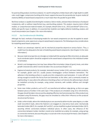
![Modelling Guide for Timber Structures
Structural component analysis - Chapter 4.2
3
4.2.3 Tension Components
Common tension (parallel to grain) components include webs and bottom chords of trusses (see Figure 1),
bottom flanges in wood I-joists, chord members in diaphragms, end studs of shear walls, and occasionally
bracingmembers. The bottom chordsof trusses are often loaded in axial tension combined with bending. This
section deals only with axially loaded members.
Figure 1. Timbertruss
4.2.3.1 Analytical Methods
Analysis of a component under axial tension is relatively straightforward. The tensile resistance, Tr, of the
componentcan be calculated using Equation 1:
𝑻𝑻𝒓𝒓 = 𝒇𝒇𝒕𝒕𝑨𝑨 [1]
where ft is the axial tensile strength of the component. This axial tensile strength must take into account the
load-duration effect,service condition effect, size effect,treatment effect,and system effectaccordingto the
testing results or design standards, such as CSA O86 (CSA Group, 2019). A is the cross-sectional area of the
component. More than one cross-section is typically assessed when the cross-sectional areaof components is
not uniform or when cross-sectionsare weakened by, for example, fasteners.
CSA O86 only takes into account the size effectof the cross-section for sawn lumber and not the length effect.
The design value of the gross section of glulam components has been decreased to compensate for the size
effect.The National Design Specification (NDS) (American Wood Council,2018) doestake the size effectof the
cross-section into accountfor sawn lumber,and both the size effectof the cross-section and the length effect,
called volume effect,for glulam. EN 1995-1-1 (CEN,2009) takesinto accountthe size effectof the cross-section
for sawn timber and for glulam, and both the size effectof the cross-section and the length effectfor LVL.
The deformation, Δ, of the component under axial tension force,F, can be calculated using Equation 2:
∆=
𝑭𝑭𝑭𝑭
𝑨𝑨𝑨𝑨
[2]](https://image.slidesharecdn.com/modellingguidefortimberstructures-240325073901-2a07d971/85/Modelling-Guide-for-Timber-Structures-FPInnovations-131-320.jpg)


![Modelling Guide for Timber Structures
Structural component analysis - Chapter 4.2
7
Table 2. Minimum design valuesofeffective-length factor,Ke,for compression members(CSA Group,2019)
Degree ofend restraint ofcompression member Ke Symbol
Effectively held in position and restrained against rotation at both ends 0.65
Effectively held in position at both ends and restrained against rotation at
one end
0.80
Effectively held in position at both ends but not restrained against rotation 1.00
Effectively held in position and restrained against rotation at one end, and
restrained against rotation but not held in position at the other end
1.20
Effectively held in position and restrained against rotation at one end, and
partially restrained against rotation but not held in position at the other end
1.50
Effectively held in position but not restrained against rotation at one end,
and restrained against rotation but not held in position at the other end
2.00
Effectively held in position and restrained against rotation at one end but
not held in position or restrained against rotation at the other end
2.00
Note: Effective length L = KeLo, where Lo is the distance between the centres of lateral supports of the
compression member in the plane in which buckling is beingassessed.
Traditionally, the analysis and design of columns is in three parts: a constant crushing capacity for short
columns; an empirical curve for intermediate lengths; and a Euler formula for long columns (Johns, 2011).
Nowadays, a single curve for the column stability (or slenderness) factor, aimed at reducingdesign strengths
due to buckling, is typically adopted for all slendernessratios.Take the CSA O86,for example: a formula based
on the cubic Rankine-Gordon curve (Figure 6) isused to obtain the resistance of axial compression components.
Figure 6. Tangent cubicRankine-Gordon and Eulerformulaversuscolumn data(Zahn,1989)
The resistance,Pr, of the compression componentcan be calculated using Equation 3:
𝑷𝑷𝒓𝒓 = 𝒇𝒇𝒄𝒄𝑨𝑨𝑲𝑲𝒁𝒁𝒁𝒁𝑲𝑲𝑪𝑪 [3]](https://image.slidesharecdn.com/modellingguidefortimberstructures-240325073901-2a07d971/85/Modelling-Guide-for-Timber-Structures-FPInnovations-135-320.jpg)


![Modelling Guide for Timber Structures
Chapter 4.2 - Structural component analysis
12
Figure 11. Lateral-torsionalbucklingofasimplysupported beam (CourtesyofAmerican Wood Council)
Unlike compression components, bendingcomponents sometimes have narrow cross-sectionsto resist shear
forces, as in the case of prefabricated wood I-joists with oriented strand board (OSB) webs. The bending
componentsthen have to take into account global buckling(lateral-torsional buckling) as well as local buckling
in the webs (see Figure 12). Analytical methods can usually take into account global buckling, but only rarely
local buckling,which typically has to be analysed using FE methods.
(a) (b)
Figure 12. Two typicalbucklingmodesofI-joists(Zhu et al.,2005): (a)global; and (b)localbuckling
Typically, the analysis and design of the bendingresistance of beams (e.g., using CSA O86) fall under one of the
three parts: a constant material strength; a curve for the inelastic buckling; or a curve for linear buckling
(Hooley & Madsen, 1964). NDS has adopted a similar approach. The bending moment resistance, Mr, of
bendingcomponents can be calculated using Equation 4:
𝑴𝑴𝒓𝒓 = 𝒇𝒇𝒃𝒃𝑺𝑺𝑲𝑲𝒁𝒁𝒁𝒁𝑲𝑲𝑳𝑳 [4]](https://image.slidesharecdn.com/modellingguidefortimberstructures-240325073901-2a07d971/85/Modelling-Guide-for-Timber-Structures-FPInnovations-140-320.jpg)
![Modelling Guide for Timber Structures
Structural component analysis - Chapter 4.2
13
where fb is the bending strength of the component. This bending strength must take into account the load-
duration effect,service condition effect,treatmenteffect,and system effectaccordingto the testing results or
design standards (e.g., CSA O86). S is the section modulus of the component. 𝐾𝐾𝑍𝑍𝑍𝑍 and 𝐾𝐾𝐿𝐿 are the size factor
and lateral stability factor, respectively, and are determined using different equations depending on the
product type and design standards. Note that the KL factor was developed for simply-supported single-span
beams with rectangular sections and an E/G ratio (MOE divided by the shear modulus) of 16, without taking
into account the lateral bracing provided by sheathing or decking, under transverse loads applied on the top
flange. When design conditionsare not aligned with these assumptions, FE modelling is more favourable.
Aside from the bending resistance, the shear resistance of beams also needs to be analysed or verified. The
shear resistance, Vr, of bending componentscan be calculated using Equation 5:
𝑽𝑽𝒓𝒓 = 𝒇𝒇𝒗𝒗
𝟐𝟐𝑨𝑨𝒏𝒏
𝟑𝟑
𝑲𝑲𝒁𝒁𝒁𝒁 [5]
where fv is the shear strength of the component. This shear strength must take into accountthe load-duration
effect, service condition effect, treatment effect, and system effect accordingto the testing results or design
standards (e.g., CSA O86). 𝐴𝐴𝑛𝑛 is the net cross-sectional area of the component. 𝐾𝐾𝑍𝑍𝑍𝑍 is the size factor and is
determined using differentequations dependingon the producttype and design standards.
The deflection of the bending components can be calculated using engineering principles, for example, the
moment theorem method, or the equations provided by some design handbooks, for example, Wood Design
Manual 2020 (Canadian Wood Council,2021).When analysingmostof the wood materials used in construction,
deformation caused by shear is not commonly computed to simplify the analytical models. Except in special
cases, the shear modulus for concrete and steel is high enough to assume that the shear deformation is too
small to be relevantor worth computing. For most common wood products, the E/G ratio is approximately 16,
far above the ratio of 2 to 3 observed in concrete and steel.For this reason, design standards such as CSA O86
and NDS (American Wood Council, 2018) provide an apparent MOE, which is historically reduced from the
measured MOE to include shear deformation effects. These standards also specify how to get a shear-free (or
true) MOE. This apparent MOE applies to simple-span beams with a span-to-depth ratio between 17:1 and
21:1 (See American Wood Council, NDS-2018 Appendix F.3). Proportion between shear deformation and
bending deformation varies depending on loading and support conditions, beam geometry, span, and the
effective shear stiffness. In some cases, such as a deep beam or a cantilever, it is better to compute shear
deformations separately as the shear deformations calculated based on the apparent MOE may not be
accurate.
Shear deformation of wood productssuch as CLT panels is higher than for other products, mainly because of
the rolling shear of the transverse layers.The same is true of other engineered wood productswith a low shear
modulus. Both CSA O86 (Clause 8.5.2) and NDS (Clause 10.4.1) specify to compute both shear and bending
deformation, but do not provide guidance or equationsto cover all design cases. In addition, most of the beam
deformation equations in the literature are for bending-only deformations; it is rare for these equations to
show the shear part of the deformation. For these engineered wood products, it is important either to design
with analytical modelsthat include shear deformation or to use a software program capable of analysing shear
deformation of materials. In all cases, when a software program with user-defined materials computes shear
deformation, it is important to provide a shear-free MOEas an entry parameter.](https://image.slidesharecdn.com/modellingguidefortimberstructures-240325073901-2a07d971/85/Modelling-Guide-for-Timber-Structures-FPInnovations-141-320.jpg)


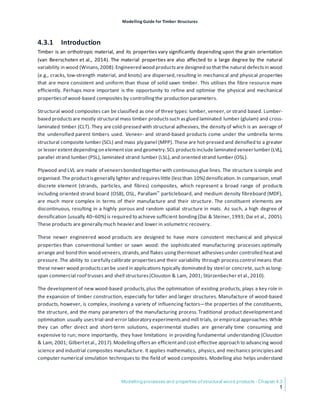

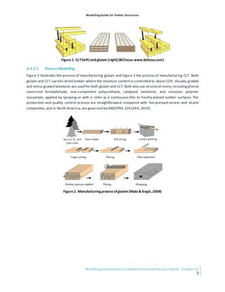


![Modelling Guide for Timber Structures
Chapter 4.3 - Modelling processes and properties of structural wood products
8
4.3.2.2.1.2 Advanced FE Models
Optical scanning devices can determine the orientation of fibre on the surface of lumber, as illustrated in
Figure 8. The information on fibre angle in combination with a micromechanical model for wood can be used
to generate longitudinal stiffness and strength profilesof each lamella. These property profilescan be used to
develop an advanced FE modelling method for predicting the mechanical performance of glulam. This
modellingapproach includesfour basic steps: (1) laser scanning; (2) reconstruction of 3D fibreand knotmodels;
(3) determination of stiffness and strength profiles; and (4) analysis.
Figure 8. Tracheid effectand itsexploitation in laser scanning(Kandler,Lukacevic,Zechmeister,et al.,2018):
(a) setup; (b)scanningthe woodensurface;(c)visualisation ofarecorded shape;(d)the wooden surface;(e)
fittingofthe ellipse; (f)estimatingtheout-of-planecomponent ofthefibre;and (g)resultantvector file offibre
angle measurements
The first step, laser scanning, describespropagation of light in wood, based on the tracheid effect.A simplified
setup comprisesalaser and a camera, as shown in Figure 8(a). Light travelsfurther in adirection parallel to the
fibre than perpendicular to the fibre in wood. Thus, projecting a laser dot onto a wooden surface and
decomposing the spread of the light reveals the major material axis (see Figures 8[d] and 8[e]). While the in-
plane fibre angle can be measured this way in principle only,Kandler,Füssl, Serrano & Eberhardsteiner (2015)
presented approaches to deduct the out-of-plane angle from the same dataset (see Figures 8[f] and 8[g]) by
using the ratio between the minor and major axes of the ellipse to estimate the out-of-plane component of
the fibre.
A weak-zone approach (Fink et al., 2013) is used to construct the laminae. Each lamina is modelled using
undisturbed,defect-free clearwood sections.These are interrupted by weak sectionsrepresentingknotgroups
and defects. To reconstruct knot morphology, the resulting fibre angle values are used to automatically
determine knot areas on all four surfaces of the board. The 3D knot geometry is reconstructed using an
automated algorithm where the knots are modelled asrotationally symmetric cones(illustrated in Figure 9[a]).](https://image.slidesharecdn.com/modellingguidefortimberstructures-240325073901-2a07d971/85/Modelling-Guide-for-Timber-Structures-FPInnovations-155-320.jpg)


![Modelling Guide for Timber Structures
Chapter 4.3 - Modelling processes and properties of structural wood products
22
Figure 27. Exampleofmodellingtheeffectoffeed rateon productionefficiencyusingVDry
4.3.3.1.5 Veneer Grading and ProductLayup
For structural plywood and LVL products,veneer stress-gradingiscritical to ensure productpropertiesconform
to industry standards APA PS-1 (2010) and ASTM D5456 (2021).The stress grade of veneer dependsmainly on
grain angle and wood density. These characteristics are available for download when using an industry
standard machine such as the Metriguard veneer scanner,which also measures veneer moisture content and
temperature.The VGrader model inputs the data collected by the Metriguard scanner for each sheet(density,
moisture content,temperature,ultrasonic propagation time [UPT]) to outputthe veneer MOEor E-grade based
on density and grain orientation, which is directly correlated to UPT(Wang & Dai, 2013).The VGrader software
also produces grade out-turn distributions based on input species, and E-grade or thresholds of UPT value
straight from the Metriguard data, as illustrated in Figure 28.](https://image.slidesharecdn.com/modellingguidefortimberstructures-240325073901-2a07d971/85/Modelling-Guide-for-Timber-Structures-FPInnovations-169-320.jpg)
![Modelling Guide for Timber Structures
Modelling processes and properties of structural wood products - Chapter 4.3
23
Figure 28. Schematicoflinkage betweenmilldatafrom Metriguard veneerscanningand VGradersimulation
software analyses: UPTstandsfor ultrasonicpropagation time,Temp for temperature,MOEfor modulusof
elasticity,MC for moisture content,Den for density,Ave for average,Min for minimum,and PLW forplywood
The VGrader simulator was designed to model the effects on average and variability (standard deviation, or
stdev) of veneer MOEby togglingbetween veneer visual grade or MOEgrade distributions(Figure 29[a]).Visual
grade isgenerally no indicator of the MOEof a veneer,which isbased on the UPTand density. Based on classical
lamination theory, the VGrader predictsthe product-bendingMOE and modulus of rupture (MOR) of plywood
or LVL by E-grade of veneer layersand their layup (Figure 29[b]).The standard practice isto locate the highest
(G1) veneers in the surface layers and the lowest (G3) veneers in the core to maximise the panel-bending
strength and usage of all veneer grades.](https://image.slidesharecdn.com/modellingguidefortimberstructures-240325073901-2a07d971/85/Modelling-Guide-for-Timber-Structures-FPInnovations-170-320.jpg)


![Modelling Guide for Timber Structures
Chapter 4.3 - Modelling processes and properties of structural wood products
36
Figure 40. Actualand idealised PSLmesostructure (Arwadeetal.,2010).Note: ϴ isgrain orientationangle
4.3.4.3.2 Integrated Model for Strand-based Products
Barnes (2000) developed a foundational semi-empirical model to predict the strength properties of oriented
strand and particleboardsusing input wood properties(density, MOE, MOR) and eight parameters related to
process: wood content; strand length; strand thickness; in-plane strand orientation; fines content; resin
content; gaps between disc orienteer vanes; and strand free-fall distance from former surface to mat surface.
Strand length and thicknessinteract strongly to affect the efficiency of the composite as it reachessolid parent
wood strength (Figure 41[a]), showing how a high slendernessratio is most effective,and the practical upper
range of strand length is 6″ (152 mm). The grain angle orientation in the mat is the other adjustable parameter
that significantly affectsthe ability of the composites to approach parent wood MOE (Figure 41[b]). The model
doesnot incorporate aVDP effect.
( a) ( b )
Figure 41. Examplesofkeyprocessparameter effectson OSBcompositeefficiency: (a)strand length and
thickness,and (b)in-plane orientation angle in mat (Barnes,2000)
Building on these process models, FPInnovations developed OSB-Pro, an integrated model for predicting the
mechanical properties of strand composites of OSB/LSL. Key steps and factors involving strand preparation,
strand orientation, mat forming, and mat consolidation in thismodel and the finished strand productare shown
in the flowchart in Figure 42. The model contains nine modules including the input and output modules. For
the model input, specific parameters related to raw materials and production processes are required:
dimensions, density, and moisture content of panels; dimensions, density, and MOE of strands; number of
layers; average angle of strands in each layer; VDP parameters; resin content; and fines content. Ultimately,
the model can calculate mean values of axial, flatwise, and edgewise (in the case of LSL) bending MOEs.](https://image.slidesharecdn.com/modellingguidefortimberstructures-240325073901-2a07d971/85/Modelling-Guide-for-Timber-Structures-FPInnovations-183-320.jpg)


![Modelling Guide for Timber Structures
Modelling processes and properties of structural wood products - Chapter 4.3
43
Future models should focuson accurately characterisingmaterial propertiesbased on the structural, physical,
and mechanical variations in raw materials, cutting-induced damage to wood constituents, and bonding and
failure mechanism of the final products. Better knowledge in these areas will lead to more accurate model
inputs and validations. Data-driven modelling, which we do not discuss in detail here, has great potential for
practical applications, particularly in processoptimisation.
4.3.6 Acknowledgements
The authors would like to acknowledge Dr. Kate Semple and Dr. Meiling Chen for their contributions to this
chapter.
4.3.7 References
Amini, A., Arwade, S. R., & Clouston, P. L. (2017). Modeling the effect of void shapes on the compressive
behavior of parallel-strand lumber. Journal of Materials in Civil Engineering, 29(9), 04017129.
https://doi.org/10.1061/(ASCE)MT.1943-5533.0001980
André,N., Cho, H. W., Baek, S. H., Jeong, M. K., & Young, T. M. (2008).Prediction of internal bond strength in
a medium density fiberboard process using multivariate statistical methods and variable selection.
Wood Science and Technology, 42(7),521-534.https://doi.org/10.1007/s00226-008-0204-7
APA. (2019). ANSI/APA PRG 320: Standard for performance-rated cross-laminated timber. The Engineered
Wood Association (APA).
Arwade, S. R., Clouston, P. L., & Winans, R. (2009). Measurement and stochastic computational modeling of
the elastic properties of parallel strand lumber. Journal of Engineering Mechanics, 135(9), 897-905.
https://doi.org/10.1061/(ASCE)EM.1943-7889.0000020
Arwade, S. R., Winans, R., & Clouston, P. L. (2010). Variability of the compressive strength of parallel strand
lumber. Journal of Engineering Mechanics, 136(4),405-412.https://doi.org/10.1061/(ASCE)EM.1943-
7889.0000079
APA.(2010).APA PS 1 Voluntary productstandard, Structural plywood. Engineered Wood Association (APA).
ASTM. (2018).ASTM D3737-18e1: Standard practice for establishing allowable properties for structural glued
laminated timber (glulam). ASTM International. https://doi.org/10.1520/D3737-18E01
ASTM. (2021). ASTM D5456-21e1: Standard specification for evaluation of structural composite lumber
products. ASTM International.
Barnes, D. (2000). An integrated model of the effect of processing parameters on the strength properties of
oriented strand wood products. Forest Products Journal, 50(11/12),33-42.
Bejo, L., & Lang, E. M. (2004). Simulation based modeling of the elastic properties of structural composite
lumber. Wood and Fiber Science, 36(3),395-410.
Bender, D. A., Woestee, F. E., Schaffera, L., Marx, N. (1985). Reliability formulation for the strength and fire
endurance of glued-laminated beams. Research paper FPL-460,U.S.D.A. Forest Products Laboratory.
Blass H. J., & Fellmoser, P. (2004, June 14–17). Design of solid wood panels with cross layers [Conference
presentation]. World Conference on Timber Engineering,Lahti, Finland.
Brandner, R., Flatscher, G., Ringhofer, A., Schickhofer, G., & Thiel, A. (2016). Cross laminated timber (CLT):
overviewand development.Holz als Roh- und Werkstoff, 74(3),331-351.
Brown, K. M., & Suddarth, S. K. (1977).A glued laminated beam analyzer for conventional or reliability based
engineering design. Purdue University Agricultural Experiment Station.
Burk, A. G. (1988). Reliability models for finger joint strength and stiffness properties in Douglas-fir visual
laminating grades. [Master’s thesis, Texas A&M University].](https://image.slidesharecdn.com/modellingguidefortimberstructures-240325073901-2a07d971/85/Modelling-Guide-for-Timber-Structures-FPInnovations-190-320.jpg)
![Modelling Guide for Timber Structures
Chapter 4.3 - Modelling processes and properties of structural wood products
44
Burk, A. G., & D. A.Bender.(1989).Simulating finger-joint performance based on localized constituent lumber
properties.Forest Products Journal, 39(3),45-50.
Carvalho, L. M. H., & Costa, C. A. V. (1998) Modeling and simulation of the hot-pressing process in the
production of medium density fibreboard (MDF).Chemical Engineering Communications,170(1),1-21.
https://doi.org/10.1080/00986449808912732
Cha, J. K., & Pearson,R. G. (1994).Stressanalysis and prediction in 3-layer laminated veneer lumber: Response
to crack and grain angle. Wood and Fiber Science, 26(1),97-106.
Chen,M., Troughton, G., & Dai, C. (2021).Optimumveneer peelingtemperaturesfor selected softwood species
usingbig roller bars.HolzalsRoh- und Werkstoff,79(1),151-159.https://doi.org/10.1007/s00107-020-
01619-5
Chen,Z., Ni, C., Dagenais, C., & Kuan,S. (2020).WoodST: A temperature-dependentplastic-damage constitutive
model used for numerical simulation of wood-based materials and connections. Journal of Structural
Engineering, 146(3),A04019225.https://doi.org/10.1061/(ASCE)ST.1943-541X.0002524
Clouston, P. (2007). Characterization and strength modeling of parallel-strand lumber. Wood Research and
technology, 61(4),394-399.https://doi.org/10.1515/HF.2007.052
Clouston, P. L., & Lam, F. (2001). Computational modeling of strand-based wood composites. Journal of
Engineering Mechanics, 127(8),844-851.https://doi.org/10.1061/(ASCE)0733-9399(2001)127:8(844)
Clouston, P. L., & Lam, F. (2002).A stochastic plasticity approach to strength modeling of strand-based wood
composites. Composites Science and Technology, 62(10-11), 1381-1395.
https://doi.org/10.1016/S0266-3538(02)00086-6
Colling, F. (1990). Biegefestigkeit von brettschichtholzträgern in abhängigkeit von den festigkeitsrelevanten
einflußgrößen [Bendingstrength of glulam beams. Development of a statistical model]. Holz als Roh-
und Werkstoff, 48, 269-273.https://doi.org/10.1007/BF02626515
Coumans, E. (2010).Bullet2.76 PhysicsSDK Manual. Bullet PhysicsLibrary.http://bulletphysics.org
Coumans, E. (2015, August 9–11). Bullet Physics Simulation: Introduction to rigid body dynamics and collision
detection [Conference presentation]. 42nd International Conference and Exhibition on Computer
Graphics and Interactive Techniques,Los Angeles,California, USA.
Dai, C. (1994).Modelling structure and processing characteristics of a randomly-formed wood-flakecomposite
mat. [Doctoral thesis, University of British Columbia].
Dai, C. (2001). Viscoelastic behavior of wood composite mats during consolidation. Wood and Fibre Science,
33(3),353-363.
Dai, C., Chen, S . and Sallahuddin, U. 1996. LOGCON 2.0: Dynamic software for log conditioning.
Forintek copyright.
Dai, C., & Steiner, P. R. (1993). Compression behavior of randomly formed wood flake mats. Wood and Fiber
Science, 25(4), 349-358.
Dai, C., & Steiner,P. R. (1994).Spatial structure of wood compositesin relation to processingand performance
characteristics.Wood Science and Technology, 28(3),229-239.https://doi.org/10.1007/BF00193331
Dai, C., & Steiner,P. R. (1997).On horizontal density variation in randomly-formed short-fibre wood composite
boards. Composites. Part A: Applied Science and Manufacturing, 28(1), 57-64.
https://doi.org/10.1016/S1359-835X(96)00094-2
Dai, C., & Yu, C. (2004).Heatand mass transfer in wood composite panelsduringhot-pressing: PartI.A physical-
mathematical model. Wood and Fiber Science, 36(4),585-597.](https://image.slidesharecdn.com/modellingguidefortimberstructures-240325073901-2a07d971/85/Modelling-Guide-for-Timber-Structures-FPInnovations-191-320.jpg)
![Modelling Guide for Timber Structures
Modelling processes and properties of structural wood products - Chapter 4.3
45
Dai, C., & Yu, C. (2008). Modeling concentrated static load (CSL) properties of OSB. FPInnovations-Forintek
report#4568.FPInnovations.
Dai, C., Semple, K., Chow, G., & Allison, B. (2017). Developing a veneer clip (VClip) simulator for clipping
optimization. Record #: FPIPRODUCT-173-1334.FPInnovations.
Dai, C., van den Doel,K., Semple,K., Groves,K., Greig,G., & Perraud,F.(2017).Development of strand orienting
simulator (SOS) for engineered wood products. Record #: FPIPRODUCT-173-1358.FPInnovations.
Dai, C., Yu, C., Groves, K., & Lohrasebi, H. (2007). Theoretical modeling of bonding characteristics and
performance of wood composites: Part 2. Resin distribution. Wood and Fiber Science, 39(1),56-70.
Dai, C., Yu, C.,& Hubert,P.(2000,December 10–13).Modeling vertical density profilein wood compositeboards
[Conference presentation].Pacific Rim Bio-based Composites Symposium, Canberra,Australia.
Dai, C., Yu, C., & Jin, Q. (2008). Theoretical modeling of bonding characteristics and performance of wood
composites: Part IV. Internal bond strength. Wood and Fiber Science, 40(2),146-160.
Dai, C., Yu, C., Wang,B., & Xu, H. (2004).Physical and mechanical modelsfor wood strand composites.Canadian
Forest Services.
Dai, C., Yu, C., Xu, C., & He, G. (2007).Heat and mass transfer in wood composite panels during hot pressing:
Part IV. Experimental investigation and model validation. Holzforschung, 61(1), 83-88.
https://doi.org/10.1515/HF.2007.013
Dai, C., Yu, C., & Zhou, C. (2007). Theoretical modeling of bonding characteristics and performance of wood
composites. Part I. Inter-elementcontact. Wood and Fiber Science, 39(1),48-55.
Dai, C., Yu, C., & Zhou, X. (2005).Heat and mass transfer in wood composite panels duringhot pressing. Part II.
Modeling void formation and mat permeability. Wood and Fiber Science, 37(2),242-257.
Dartois, S., Nadot-Martin, C., Halm, D., Dragon, A., Fanget, A., & Contesse, G. (2013). Micromechanical
modelling of damage evolution in highly filled particulate composites–Induced effects at different
scales. International Journal of Damage Mechanics, 22(7), 927-966.
https://doi.org/10.1177/1056789512468916
de Oliveira, S. J. C., Bolmin, O., Arrigoni, M., & Jochum, C. (2018). Plywood experimental investigation and
modeling approach for static and dynamic structural applications. In A.Öchsner & H. Altenbach (Eds.),
Improved performance of materials. Springer.
Defo, M., & Brunette,G. (2007).Application of a mathematical model to the analysis of the influence of length
and diameter on log dryingrate. Wood and Fiber Science, 39(1),16-27.
Dixon, P. G., Malek, S., Semple, K. E., Zhang, P. K., Smith, G. D., & Gibson, L. J. (2017).Multiscale modelling of
moso bamboo oriented strand board. BioResources, 12(2), 3166-3181.
https://doi.org/10.15376/biores.12.2.3166-3181
Dodson, C. T. J. (1971). Spatial variability and the theory of sampling in random fibrous networks. Journal of
the Royal Statistical Society: Series B. Methodological, 33(1), 88-94. https://doi.org/10.1111/j.2517-
6161.1971.tb00859.x
Drolet, F., & Dai, C. (2010).Three-dimensional modelingof the structure formation and consolidation of wood
composites. Holzforschung, 64(5), 619-626.https://doi.org/10.1515/hf.2010.080
Ehlbeck, J., Colling, F., & Görlacher, R. (1985). Einfluß keilgezinkter lamellen auf die biegefestigkeit von
brettschichtholzträgern [Influence of fingerjointed lamellae on the bendingstrength of glulambeams].
Holz als Roh-und Werkstoff, 43,333-337.https://doi.org/10.1007/BF02607817
Ek, J., & Norbäck, V. (2020).Modeling of laminated veneer lumber: A study of the material properties for thick
structural elements. [Master’s thesis, Chalmers University of Technology].](https://image.slidesharecdn.com/modellingguidefortimberstructures-240325073901-2a07d971/85/Modelling-Guide-for-Timber-Structures-FPInnovations-192-320.jpg)
![Modelling Guide for Timber Structures
Chapter 4.3 - Modelling processes and properties of structural wood products
46
El Moustaphaoui, A., Chouaf, A., Kimakh, K., & Chergui, M. H. (2020). Determination of the onset and
propagation criteria of delamination of Ceiba plywood by an experimental and numerical
analysis. Wood Material Science and Engineering, 16(5), 1-11.
https://doi.org/10.1080/17480272.2020.1737963
Fink,G., Frangi,A., & Kohler,J.(2013,August26–29).Modellingthe bendingstrength of glued laminated timber
- considering the natural growth characteristics of timber [Conference presentation]. W018 Meeting
on Timber Structures,Vancouver,Canada.
Folz, B., & Foschi, R. O. (1995). ULAG: Ultimate load analysis of Glulam – User’s manual, Version 1.0.
Department of Civil Engineering,The University of British Columbia.
Foschi, R.O. (1976).Log centeringerrorsand veneer yield.Forest Products Journal,26(2), 52-56.
Foschi,R. O., & Barrett,J. D. (1980).Glued-laminated beam strength: amodel. Journal of theStructural Division,
106(ST8),1735-1754.https://doi.org/10.1061/JSDEAG.0005496
Franzoni,L., Lebée,A.,Lyon,F.,& Forêt,G. (2017).Elastic behavior of crosslaminated timber and timber panels
with regular gaps: Thick-plate modeling and experimental validation. Engineering Structures, 141,402-
416.https://doi.org/10.1016/j.engstruct.2017.03.010
Freas, A. D., & Selbo, M. L. (1954). Fabrication and design of glued laminated wood structural members.
Technical Bulletin No. 1069.U.S.D.A. Forest Products Laboratory.
Geers,M. G., Kouznetsova, V. G., & Brekelmans, W. A. M. (2010).Multi-scale computational homogenization:
Trends and challenges. Journal of Computational and Applied Mathematics, 234(7), 2175-2182.
https://doi.org/10.1016/j.cam.2009.08.077
Gereke,T., Malekmohammadi, S., Nadot-Martin, C., Dai, C., Ellyin, F., & Vaziri, R. (2012).Multiscale stochastic
modeling of the elastic properties of strand-based wood composites. Journal of Engineering
Mechanics, 138(7),791-799.https://doi.org/10.1061/(ASCE)EM.1943-7889.0000381
Gibson, L. J., & Ashby M. F. (1988). Cellular solids: Structure and Properties. Pergamon Press.
https://doi.org/10.1002/adv.1989.060090207
Gilbert,B. P. (2018).Compressive strength prediction of veneer-based structural products.Journal of Materials
in Civil Engineering, 30(9),04018225.https://doi.org/10.1061/(ASCE)MT.1943-5533.0002417
Gilbert, B. P., Bailleres, H., Zhang, H., & McGavin, R. L. (2017).Strength modelling of laminated veneer lumber
(LVL) beams. Construction and Building Materials, 149, 763-777.
https://doi.org/10.1016/j.conbuildmat.2017.05.153
Govindarajoo, R. (1989). Simulation modeling and analyes of straight horizontally-laminated timber beams.
[Doctoral dissertation, Purdue University].
Harris, R. A., & Johnson, J. A. (1982). Characterization of flake orientation in flakeboard by the von Mises
probability distribution function. Wood and Fiber Science, 14(4),254-266.
Han, G., Wu, Q., & Lu, J. Z. (2007). The influence of fines content and panel density on properties of mixed
hardwood oriented strandboard. Wood and Fiber Science, 39(1),2-15.
He, G., Yu, C., & Dai, C. (2007). Theoretical modeling of bonding characteristics and performance of wood
composites. Part 3: Bonding strength between two wood elements. Wood and Fiber Science, 39(4),
566-577.
Hernandez, R., Bender, D. A., Richburg, B. A., & Kline, K. S. (1992). Probabilistic modeling of glued-laminated
timber beams. Wood and Fiber Science, 24(3), 294-306.](https://image.slidesharecdn.com/modellingguidefortimberstructures-240325073901-2a07d971/85/Modelling-Guide-for-Timber-Structures-FPInnovations-193-320.jpg)
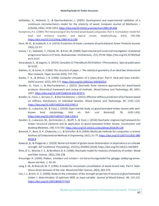
![Modelling Guide for Timber Structures
Chapter 4.3 - Modelling processes and properties of structural wood products
48
Li, M., Füssl, J., Lukacevic,M., Martin, C., & Eberhardsteiner,J. (2018). Bending strength predictionsof cross-
laminated timber plates subjected to concentrated loading using 3D finite-element-based limit
analysis approaches. Composite Structures, 220, 912-925.
https://doi.org/10.1016/j.compstruct.2019.02.101
Malek, S. (2014). Efficient multi-scale modelling of viscoelastic composites with different microstructures.
[Doctoral dissertation, University of British Columbia].
Malek, S., Gereke, T., Zobeiry, N., & Vaziri, R. (2018, January 31–February 2). Multi-scale modelling of time-
dependent response of composite structures made of orthotropic viscoelastic materials [Conference
presentation]. 13th International Conference on Steel, Space and Composite Structures, Perth,
Australia.
Malek, S., Nadot-Martin, C., Tressou, B., Dai, C., & Vaziri, R. (2019). Micromechanical modeling of effective
orthotropic elastic and viscoelastic properties of parallel strand lumber using the morphological
approach. Journal of Engineering Mechanics, 145(9), 04019066.
https://doi.org/10.1061/(ASCE)EM.1943-7889.0001631
Malek, S., Zobeiry, N., Dai, C., & Vaziri, R. (2019). Strain-softening response and failure prediction in notched
oriented strand board. Journal of Materials in Civil Engineering, 31(6), 04019094.
https://doi.org/10.1061/(ASCE)MT.1943-5533.0002737
Malek, S., Zobeiry, N., Gereke, T., Tressou, B., & Vaziri, R. (2015). A comprehensive multi-scale analytical
modelling framework for predicting the mechanical properties of strand-based composites. Wood
Science and Technology, 49(1),59-81.https://doi.org/10.1007/s00226-014-0682-8
Malekmohammadi, S., Tressou, B., Nadot-Martin, C., Ellyin, F., & Vaziri, R. (2014). Analytical micromechanics
equations for elastic and viscoelastic properties of strand-based composites. Journal of Composite
Materials, 48(15),1857-1874.https://doi.org/10.1177/0021998313490977
Malo, K.A. & Angst, V. (2008).Glued laminated timber. In Leonardo da Vinci Pilot Project,Handbook 1 - Timber
Structures, CZ/06/B/F/PP/168007.
Mäntylä, M. (1988).An introduction to solid modelling. In Principlesof computer science principles,Computer
Science Press.
Merhar, M. (2020). Determination of elastic properties of beech plywood by analytical, experimental and
numerical methods. Forests, 11(11),1221.https://doi.org/10.3390/f11111221
Nadot‐Martin, C., Touboul, M., Dragon, A., & Fanget, A. (2008).Directscale transition approach for highly‐filled
viscohyperelastic particulate composites: Computational study. In: Cazacu O (Ed.) Multiscale modeling
of heterogenous materials: From microstructure to macro-scale properties, London: ISTE/Wiley.
Nairn, J. A. (2003).Material point method calculations with explicitcracks. Computer Modeling in Engineering
and Sciences,4(6),649-664.
Noffsinger, J.R. (2004). Modeling the oriented strandboard manufacturing process and the oriented
strandboard continuous rotary drying system. [Doctoral thesis, West Virginia University].
https://doi.org/10.33915/etd.2104
Perret, O., Lebée, A., Douthe, C., & Sab, K. (2019). Equivalent stiffness of timber used in CLT: closed-form
estimates and numerical validation. Holz als Roh- und Werkstoff, 77, 367-379.
https://doi.org/10.1007/s00107-019-01395-x
Pineda,H., Hu,Y., Semple,K., Chen,M., & Dai, C. (2021).Computer simulation of the mat formation of bamboo
fibre composites. Composites Part A: Applied Science and Manufacturing, 149, 106542.
https://doi.org/10.1016/j.compositesa.2021.106542](https://image.slidesharecdn.com/modellingguidefortimberstructures-240325073901-2a07d971/85/Modelling-Guide-for-Timber-Structures-FPInnovations-195-320.jpg)
![Modelling Guide for Timber Structures
Modelling processes and properties of structural wood products - Chapter 4.3
49
Popovski, M., Gagnon, S., Mohammad, M., & Chen,Z. (2019).Chapter 3: Structural design of cross-laminated
timber elements. In E. Karacabeyli & S. Gagnon (Eds.), Canadian CLThandbook.FPInnovations.
Richburg, B. A. (1988.) Optimization of glued-laminated beam performance. [Undergraduate fellows thesis,
Texas A&M University].
Saavedra Flores, E., Dayyani, I., Ajaj, R. M., Castro-Triguero, R., DiazDelaO, F. A., Das, R., & González Soto, P.
(2015). Analysis of cross-laminated timber by computational homogenisation and experimental
validation. Composite Structures, 121, 386-394.https://doi.org/10.1016/j.compstruct.2014.11.042
Saavedra Flores, E., Saavedra, K., Hinojosa, J., Chandra, Y., & Das, R. (2016). Multi-scale modelling of rolling
shear failure in cross-laminated timber structures by homogenisation and cohesive zone models.
International Journal of Solids and Structures, 81, 219-232.
https://doi.org/10.1016/j.ijsolstr.2015.11.027
Semple,K., & Dai, C. (2016a).Log temperature conditioning simulationsforDouglasfir and sprucepeeler blocks.
FPInnovations.
Semple, K., & Dai, C. (2016b). LogConTM log conditioning time study for Lodgepole pine peeler logs.
FPInnovations.
Semple, K., & Dai, C. (2017). Moisture evaluation and veneer peeling of Douglas fir and spruce logs from
different mills and log yard age inventories. Record #: FPIPRODUCT-173-1271.FPInnovations.
Semple, K. & Dai, C. (2018a). Mill trial of log storage age effects on veneer productivity and using LogdryTM to
predict Douglasfir residual moisture levels. FPInnovations.
Semple,K., & Dai, C. (2018b).Analysesand comparison of historic mill production data from two plywood mills.
FPInnovations.
Semple, K., & Dai, C. (2018c). Log conditioning relating theoretical data to real time data from mills and
comparing conditioning systems between two mills by species and season. FPInnovations.
Semple, K. E., & Smith, G. D. (2017). Recovery modeling for OSB strand production from hollow bamboo
culms. BioResources, 12(4),7841-7858.
Semple, K. E., Zhang, P. K., & Smith, G. D. (2015). Hybrid oriented strand boards made from Moso bamboo
(Phyllostachys pubescens Mazel) and Aspen (Populus tremuloides Michx.): Species-separated three-
layer boards. Holz als Roh- und Werkstoff, 73(4),527-536.https://doi.org/10.1007/s00107-015-0914-
0
Semple, K. E., Zhang, P. K., Smola, M., & Smith, G. D. (2015).Hybrid oriented strand boards made from Moso
bamboo (Phyllostachys pubescens Mazel) and Aspen (Populus tremuloides Michx.): uniformly mixed
single layer uni-directional boards. Holz als Roh- und Werkstoff, 73(4), 515-525.
https://doi.org/10.1007/s00107-015-0913-1
Shaler, S. M., & Blankenhorn, P. R. (1990).Composite model prediction of elastic moduli for flakeboard. Wood
and Fiber Science, 22(3),246-261.
Šmídová E, & Kabele P. (2018).Constitutive model for timber fracture used for FE simulation of LVL arch. Acta
Polytechnica CTU Proceedings, 15, 109-13.https://doi.org/10.14311/APP.2018.15.0109
Smith, G. D. (2005).Directobservation of the tumbling of OSB strands in an industrial scale coil blender.Wood
and Fiber Science, 37(1),147-159.
Steinhagen, H. P., Lee, H. W. & Loehnertz, S.P. (1987). LOGHEAT: a computer program for determining log
heating times for frozen and nonfrozen logs. Forest Products Journal, 37(11/12),60-64.](https://image.slidesharecdn.com/modellingguidefortimberstructures-240325073901-2a07d971/85/Modelling-Guide-for-Timber-Structures-FPInnovations-196-320.jpg)
![Modelling Guide for Timber Structures
Chapter 4.3 - Modelling processes and properties of structural wood products
50
Stürzenbecher, R., Hofstetter, K., Schickhofer, G., & Eberhardsteiner, J. (2010). Development of high-
performance strand boards: multiscale modeling of anisotropic elasticity. Wood Science and
Technology, 44(2),205-223.https://doi.org/10.1007/s00226-009-0259-0
Suchsland, O. (1959).An analysis of the particle board process.Michigan Quarterly Bulletin, 42(2),350-372.
Susainathan, J., Eyma, F., De Luycker,E., Cantarel, A., & Castanie, B. (2020).Numerical modeling of impact on
wood-based sandwich structures. Mechanics of Advanced Materials and Structures, 27(18), 1583-
1598.https://doi.org/10.1080/15376494.2018.1519619
Taylor, S. E. (1988). Modeling spatially correlated localized lumber properties. [Doctoral dissertation, Texas
A&M University].
Thoemen, H., Humphrey, P. E. (2003). Modeling continuous pressing for wood-based composites. Wood and
Fiber Science, 35,456-468.
Triche, M. H., & Hunt, M. O. (1993). Modeling of parallel-aligned wood strand composites. Forest Products
Journal, 43(11/12),33-44.
Tsai, S. W., & Wu, E. M. (1971). A general theory of strength for anisotropic materials. Journal of Composite
Materials, 5(1), 58-80.https://doi.org/10.1177/002199837100500106
Tsai, Y-L., & Smith, G. (2014, June 4–7). The impact of different strand configurations on the surging for a
discrete element model of oriented strand board rotary drum blender [Conference presentation].
BIOCOMP 2014,Beijing, China.
van Beerschoten,W. A., Carradine,D. M., & Carr,A. (2014).Development of constitutive model for laminated
veneer lumber using digital image correlation technique. Wood Science and Technology, 48(4), 755-
772.https://doi.org/10.1007/s00226-014-0638-z
van den Doel, K., & Dai, C. (2014).SOS: Strand orientation simulator. FPInnovations.
Vratuša, S., Kariž, M., Ayrilmis, N., & Kuzman, M. K. (2017). Finite element simulations of the loading and
deformation of plywood seat shells. Holz als Roh- und Werkstoff, 75(5), 729-738.
https://doi.org/10.1007/s00107-017-1160-4
Wang, B., & Dai, C. (2013). Development of structural laminated veneer lumber from stress graded short-
rotation hem-fir veneer. Construction and Building Material, 47, 902-909.
https://doi.org/10.1016/j.conbuildmat.2013.05.096
Wang, B., & Dai, C. (2014). Optimum log conditioning temperature pertaining to veneer peeling for four
softwood species.Research report.W-3123 Record #: FPIPRODUCT-1-7015.FPInnovations.
Wang, B. J., Ellis, S., & Dai, C. (2006).Veneer surface roughnessand compressibility pertainingto plywood/LVL
manufacturing. Part II. Optimum panel densification. Wood and Fiber Science, 38(4),727-735.
Wang, J. B., Wei, P., Gao, Z., & Dai, C. (2018). The evaluation of panel bond quality and durability of hem-fir
cross-laminated timber (CLT). Holz als Roh- und Werkstoff, 76(3),833-841.
Wang, Y-T., & Lam, F. (1998). Computational modeling of material failure for parallel-aligned strand based
wood composites. Computational Materials Science, 11(3),157-165.
Wiesner,F.,Bisby,L. A.,Bartlett, A.I., Hidalgo, J.P., Santamaria, S., Deeny,S.,& Hadden,R.M. (2019).Structural
capacity in fire of laminated timber elements in compartments with exposed timber surfaces.
Engineering Structures, 179, 284-295.https://doi.org/10.1016/j.engstruct.2018.10.084
Williamson, T., & Yeh, B. (2007, August 27–30). Standard practice for the derivation of design properties of
structural glued laminated timber in the United States [Conference presentation]. International
Council for Research and Innovation in Building and Construction, Bled,Slovenia.](https://image.slidesharecdn.com/modellingguidefortimberstructures-240325073901-2a07d971/85/Modelling-Guide-for-Timber-Structures-FPInnovations-197-320.jpg)
![Modelling Guide for Timber Structures
Modelling processes and properties of structural wood products - Chapter 4.3
51
Wilson, T. R. C., & W. S. Cottingham. (1947). Tests of glued-laminated wood beams and columns and
developmentof principle of design. Report No. R1687,U.S.D.A. Forest Products Laboratory.
Winans, R.S. (2008).Measurement and computational modeling of themechanical properties of parallel strand
lumber. [Master’s theses, University of Massachusetts Amherst].
Yeh, B. J. (1996, October 28–31). Using computer models to predict the performance of structural glued
laminated timber [Conference presentation]. International Wood Engineering Conference, New
Orleans,Louisiana, USA.
Yu, C., Dai, C., & Wang, B. (2007).Heat and mass transfer in wood composite panels duringhot pressing: Part
III. Predicted variations and interactions of the pressing variables. Holzforschung, 61, 74-82.
https://doi.org/10.1515/HF.2007.012
Zerbst, D., Liebold,C., Gereke,T., Haufe, A., Clauß, S., & Cherif,C. (2020).Modelling inhomogeneity of veneer
laminates with a finite element mapping method based on arbitrary grayscale images. Materials,
13(13),2993.https://doi.org/10.3390/ma13132993
Zhou, C., Dai, C., & Smith, G. D. (2008). A generalized mat consolidation model for wood composites.
Holzforschung, 62(2),201-208.https://doi.org/10.1515/HF.2008.053
Zhou, C., Smith, G., & Dai, C. (2010). Characterizing hydro-thermal compression behavior of aspen wood
strands. Holzforschung, 63(5),609-617.
Zombori, B. G., Kamke, F. A., & Watson, L. T. (2003). Simulation of the internal conditions during the hot-
pressingprocess.Wood and Fiber Science, 35(1), 2-23.](https://image.slidesharecdn.com/modellingguidefortimberstructures-240325073901-2a07d971/85/Modelling-Guide-for-Timber-Structures-FPInnovations-198-320.jpg)


![Modelling Guide for Timber Structures
Chapter 5 - Connections
4
The resistance of a dowel type connection is governed by either the brittle resistance of the wood fibres
engaged in resisting the load (in longitudinal shear, transverse or longitudinal tension, or a combination of
the two) or the ductile resistance which is associated with bending of the fasteners and localised crushing of
the wood fibres at the fasteners. As Figure 5 shows, the former results in a brittle failure, while the latter
results in a ductile behaviour prior to failure. However, following the onset of crushing of the fibres and
bending of the fasteners, there is always a possibility that a brittle failure occurs after large deformation. The
occurrence of this secondary failure (the brittle failure following the ductile failure) governs the amount of
ductility that the connection can provide to the structure and can also govern the maximum load that a
connection can be designed for.
(a) (b) (c)
Figure 5. Load deformation curvesfor brittle([a]and [b])and ductile (c)connection failure. The amountof
ductilityin a connection isgovernedbythe onset ofthesecondarybrittle failure
With the development of advanced seismic engineering concepts and analysis, a designer must identify the
hierarchy of structural elements that would provide the ductility in a structure. The seismic fuses or energy-
dissipative elements must be designed to provide the targeted ductility in the system. The energy-dissipation
capacity of connections can be compromised by the inherent variability in the performance of wood
elements resulting from variations in material characteristics (i.e., the 5th percentile resistance is used in the
design) and variations in construction tolerances (stronger dissipative elements are used during construction
instead of the ones specified). This is because the targeted seismic fuse behaviour may be triggered at a
much higher load and may change the behaviour of the entire system. To prevent the failure of non-
dissipative structural elements, all structural elements and connections that are not part of the hierarchy of
the identified seismic fuses must be capacity-protected. Capacity-protected elements must be designed to
accommodate the full deformation of the dissipative elements; this is commonly achieved by ensuring their
design resistance is higher than the ultimate resistance of the seismic fuse by multiplying by an overstrength
factor. The value of the overstrength factor depends on the variability of the load that triggers the seismic
fuse. It should be noted that within a dissipating fuse, it is also important to capacity-protect brittle failure
modes.](https://image.slidesharecdn.com/modellingguidefortimberstructures-240325073901-2a07d971/85/Modelling-Guide-for-Timber-Structures-FPInnovations-204-320.jpg)


![Modelling Guide for Timber Structures
Chapter 5 - Connections
12
fire performance of the assembly (Figure 13[a]). These types of connectors are generally proprietary and
their design and behaviour should be provided by the supplier or confirmed through testing.
(a) (b)
Figure 14. (a)HBV used in atimber-concretecompositefloor (TiComTecGmbH,2011),and (b)HSKused asa
hold-down in ashear wall(Zhanget al.,2018)
Figure 15. Hangerconnection system(SherpaConnectionSystems,2019)
Note that not all connections in a structure require ductility. Energy-dissipative connections require ductility,
but other connections need to meet only the strength, stiffness, and drift requirements to accommodate the
response induced by gravity and lateral loads.
Because the height of timber structures is constantly increasing with innovation, it is necessary to adapt to
the higher seismic demands in earthquake-prone zones and decrease the earthquake loadings by increasing
ductility, energy dissipation, or both, through adopting different systems. As these systems are beyond the
standard design solutions covered by timber design codes, they are defined as alternative solutions and
require special attention. Examples of such innovative systems are buckling-restrained braces and resilient
(or not) friction dampers. These systems are used to increase the timber structure’s resilience and decrease
the earthquake load demand. Figure 16 shows examples of these systems with their associated load-
deformation responses.](https://image.slidesharecdn.com/modellingguidefortimberstructures-240325073901-2a07d971/85/Modelling-Guide-for-Timber-Structures-FPInnovations-212-320.jpg)


![Modelling Guide for Timber Structures
Chapter 5 - Connections
26
Figure 30. Averageconnection maximumload and coefficient ofvariation versusnumber ofnumericalanalyses
In a connection with multiple fasteners, the variability of the wood density surrounding each fastener and the
tolerance between the fastener and the hole (e.g., for a bolted connection) influences the overall connection
load deformation. There is an element of randomness in the load transfer between the fasteners and the
timber, and only a numerical analysis in which the randomness of the parameters is taken into account could
reveal the possible average load-deformation response of a group of fasteners. Bickerdike (2006) conducted
such an analysis and assessed the sensitivity of the connection response to differentvariables.
In cases where the load-deformation response of the fasteners in a connection is highly variable as a result of
the connection configuration (e.g., the moment connection shown in Figure 2[b]), each dowel has a distinct
load-deformation relationship. The ends of the dowels are loading the column, and the middle is loading the
rafter. The column and rafter being at more or less 90 degrees to each other, and each dowel loading the
column and rafter at a specific angle to the grain, make the numerical analysis somewhat elaborated. Chui
and Li (2005) studied a similar connection geometry assuming a purely ductile behaviour with some success
but without considering the potential for any brittle wood failure (splitting or shear) to occur. Ultimately, one
would need to either consider the potential failure of the wood in the column or the rafter to be the result of
tension perpendicular to the grain stress or plainly prevent this by reinforcing the column and rafter
members to preventsplitting.
5.3.2 Screwand Glued-in-RodConnections underWithdrawal
Self-tapping screws and glued-in-rods loaded in withdrawal are types of fasteners with a significant axial
resistance. In this section, screws that resist lateral shear are not covered as these connections would be
modelled in the same manner as steel dowels, discussed in Section 5.3.1. This section covers the axial
resistance of the fasteners. The considerations discussed in this section and Section 5.3.1 should be applied
to screws which are loaded laterally and axially.
There are three types of screws used in wood construction in general: wood screws, lag screws, and
proprietary self-tapping screws (Figure 31). The design rules for wood screws and lag screws are included in
the current Canadian wood design standard (CSA O86:19). Proprietary self-tapping screws are not covered in
the current standard, but provisions are currently in development for potential inclusion in the 2024 edition.](https://image.slidesharecdn.com/modellingguidefortimberstructures-240325073901-2a07d971/85/Modelling-Guide-for-Timber-Structures-FPInnovations-226-320.jpg)
![Modelling Guide for Timber Structures
Connections - Chapter 5
27
Before the new provisions are adopted, it has been recommended that self-tapping screws be designed
based on the lag screw provisions, with some adjustments to account for the characteristics of the self-
tapping screws.
(a) (b) (c)
Figure 31. Different typesofscrews: (a)wood screw,(b)lagscrew,and (c)self-tappingscrew
Screws are often implemented in either shear (Figure 32[a]) or withdrawal (Figure 32[b]). Although using lag
screws or wood screws in pure withdrawal is uncommon, using self-tapping screws in withdrawal
configurations is common and reliable. This application results in a brittle failure mode, either in withdrawal
for shorter threaded embedment lengths, or screw steel failure in tension for longer threaded embedment
lengths. One common approach is to use inclined self-tapping screws to provide a stronger and stiffer shear
connection than a typical shear connection. Fully threaded self-tapping screws can be used to reinforce wood
in areas of high stress perpendicular to the grain as well, although no provisions for this are currently
provided in Canadian standards.
(a) (b) (c)
Figure 32. (a)Self-tappingwood screw,(b)screwin withdrawal,and (c)inclined screw in withdrawal
Glued-in rods (Serrano, 2001) are used for primarily two purposes in timber engineering: to join structural
elements (Figure 33) or to reinforce wood in areas of high tensile stress perpendicular to the grain, similar to
fully threaded self-tapping screws. Glued-in rods have been used for many years, especially for glulam — in
Europe, mainly in Nordic countries, Germany, and Russia. A glued-in-rod connection makes it possible to
obtain strong and stiff joints with excellent performance in load transfer without the need for large metal
plates (i.e., often used for other dowel type fasteners). Architects prefer concealed connection hardware for
aesthetic reasonsand for enhancingthe fire resistance of the assembly.](https://image.slidesharecdn.com/modellingguidefortimberstructures-240325073901-2a07d971/85/Modelling-Guide-for-Timber-Structures-FPInnovations-227-320.jpg)

![Modelling Guide for Timber Structures
Connections - Chapter 5
29
5.4 SUMMARY
Connections are essential elements for timber structures. This chapter discusses the structural behaviour,
failure mechanism, and design considerations of timber connections. Modelling methods and key
considerations are introduced for generic and innovative timber connections in structures that resist gravity
and lateral loads. Efficient analytical and advanced FE modelling methods are discussed for analysing
deflection, resistance, and failure modes of dowel type connections under shear, and screw and glued-in-rod
connections under withdrawal. The information presented in this chapter is intended to help practising
engineersand researchersbecome more acquainted with the analysis of timber connections.
5.5 REFERENCES
Bickerdike, M. (2006). Predicting the row shear failure mode and strength of bolted timber connections
loaded parallel-to-grain [Unpublished master’s thesis]. Royal Military College of Canada.
Chen, Z., & Popovski, M. (2020). Connection and system ductility relationship for braced timber frames.
Journal of Structural Engineering, 146(12), 4020257. https://doi.org/10.1061/(ASCE)ST.1943-
541X.0002839
Chen, Z., Ni, C., Dagenais, C., & Kuan, S. (2020). WoodST: A temperature-dependent plastic-damage
constitutive model used for numerical simulation of wood-based materials and connections. Journal
of Structural Engineering, 146(3),04019225.https://doi.org/10.1061/(ASCE)ST.1943-541X.0002524
Chen, Z., Zhu, E., & Pan, J. (2011). Numerical simulation of wood mechanical properties under complex state
of stress. Chinese Journal of Computational Mechanics, 28(4),629-634,640.
Chui, Y. H., & Li, Y. (2005). Modeling timber moment connection under reversed cyclic loading, Journal of
Structural Engineering, 131(11).https://doi.org/10.1061/(ASCE)0733-9445(2005)131:11(1757)
Computers and Structures, Inc. (2021). Material nonlinearity. Retrieved from
https://wiki.csiamerica.com/display/kb/Material+nonlinearity
CSA Group.(2019).Engineering design in wood (CSA O86:19).
Danielsson, H., & Gustafsson, P. J. (2013). A three dimensional plasticity model for perpendicular to grain
cohesive fracture in wood. Engineering Fracture Mechanics, 98, 137-152.
https://doi.org/10.1016/j.engfracmech.2012.12.008
Erki, M.-A. (1991). Modelling the load-slip behaviour of timber joints with mechanical fasteners. Canadian
Journal of Civil Engineering, 18(4).https://doi.org/10.1139/l91-074
European Committee for Standardization. (2004). Eurocode 5: Design of timber structures - Part 1-1: General -
Common rules and rules for buildings (EN 1995-1-1:2004).
Fragiacomo, M., Batchelar, M. L., Wallington, C., & Buchanan, A. (2010, June 20–24). Moment joints in timber
frames using glued-in steel rods: experimental investigation of long-term performance [Conference
presentation]. World Conference on Timber Engineering,Riva del Garda, Italy.
Franke, B., & Quenneville, P. (2011). Numerical modeling of the failure behavior of dowel connections in
wood. Journal of Engineering Mechanics, 137(3), 186-195. https://doi.org/10.1061/(ASCE)EM.1943-
7889.0000217
González Fueyo, J. L, Dominguez, M., Cabezas, J. A., & Rubio, M. P. (2009). Design of connections with metal
dowel-type fasteners in double shear. Materials and Structures, 42, 385-397.
https://doi.org/10.1617/s11527-008-9389-3](https://image.slidesharecdn.com/modellingguidefortimberstructures-240325073901-2a07d971/85/Modelling-Guide-for-Timber-Structures-FPInnovations-229-320.jpg)
![Modelling Guide for Timber Structures
Chapter 5 - Connections
30
Hashemi, A., Bagheri, H., Yousef-Beik, S. M. M., Mohammadi Darani, F., Valadbeigi, A., Zarnani, P., &
Quenneville, P. (2020). Enhanced seismic performance of timber structures using resilient
connections: Full-scale testing and design procedure. Journal of Structural Engineering, 146(9).
https://doi.org/10.1061/(ASCE)ST.1943-541X.0002749
Karacabeyli,E., & Gagnon, S. (Eds.) (2019).Canadian CLThandbook (2nd ed.).FPInnovations.
Khelifa, M., Khennane, A., El Ganaoui, M., & Celzard, A. (2016). Numerical damage prediction in dowel
connections of wooden structures. Materials and Structures, 49(5), 1829-1840.
https://doi.org/10.1617/s11527-015-0615-5
Khennane, A., Khelifa, M., Bleron, L., & Viguier, J. (2014). Numerical modelling of ductile damage evolution in
tensile and bending tests of timber structures. Mechanics of Materials, 68, 228-236.
https://doi.org/10.1016/j.mechmat.2013.09.004
Li, M., Foschi, R. O., & Lam, F. (2012). Modeling hysteretic behavior of wood shear walls with a protocol-
independent nail connection algorithm. Journal of Structural Engineering, 138(1), 99-108.
https://doi.org/10.1061/(ASCE)ST.1943-541X.0000438
National Research Council of Canada. (2020).National Building Codeof Canada.
Sandhaas, G., Van de Kuilen, J.-W., & Blass, H. J. (2012, July 15–19). Constitutive model for wood based on
continuum damage mechanics [Conference presentation]. World Conference on Timber Engineering,
Auckland,New Zealand. http://resolver.tudelft.nl/uuid:55c1c5e5-9902-43ad-a724-62bb063c3c80
Scheibmair, F., & Quenneville, P. (2014). Moment connection for quick assembly of timber portal frame
buildings: Theory and validation. Journal of Structural Engineering, 140(1).
https://doi.org/10.1061/(ASCE)ST.1943-541X.0000728
Serrano, E. (2001). Glued-in rods for timber structures — A 3D model and finite element parameter studies.
International Journal of Adhesion and Adhesives, 21(2), 115-127. https://doi.org/10.1016/S0143-
7496(00)00043-9
Sherpa Connection Systems. (2019). Design Guide. Retrieved from https://www.sherpa-
connector.com/data/082019_Bemessungsguide_EN_web.pdf
TiComTec GmbH. (2011). Load bearing constructions using wood-concrete-composite technique with glued-in
HBV-shear connectors (Technical Dossier).
Zhang, X., Popovski, M., & Tannert, T. (2018). High-capacity hold-down for mass-timber buildings. Construction
and Building Materials,164,688-703.https://doi.org/10.1016/j.conbuildmat.2018.01.019](https://image.slidesharecdn.com/modellingguidefortimberstructures-240325073901-2a07d971/85/Modelling-Guide-for-Timber-Structures-FPInnovations-230-320.jpg)


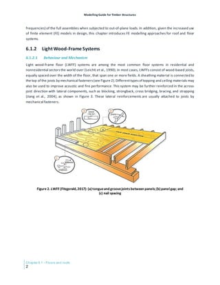
![Modelling Guide for Timber Structures
Floors and roofs- Chapter 6.1
3
Figure 3. Typicallateralreinforcements(Jianget al.,2004):(a)blocking; (b)strongback; (c)crossbridging;
(d)diagonal bracing; and (e)strapping
The main function of joists in LWFFsis to resistout-of-plane loading such as gravity load. Dependingmainly on
the loads and spans, floor joists can be installed with or without lateral bracingmembers. In braced floors,the
joists are braced against each other to increase their lateral stability and assist in load sharing. Joists are either
sawn lumber or engineered wood products, for example, laminated strand lumber (LSL), laminated veneer
lumber (LVL), wood I-joists (wooden flanges with structural panel web), or parallel chord trusses (wooden
chords with diagonal lumber or light-gauge steel elements). The selection of floor joists depends on the
strength and stiffness, with stiffness being the more dominant property in most cases due to the fact that
serviceability criteriaoften dictate the allowable floor span. Differentfloor layoutsare considered for efficiency
and cost-effectiveness.For example, 2 × 10 lumber joists are twice as stiff as 2 × 8 lumber joists and use 25%
more lumber for the same span and spacing. Conversely,2 × 10 lumber joists at 610 mm (24″) spacing are 38%
stiffer and use 16% less lumber than 2 × 8 lumber joists at 406 mm (16″) spacing (Jones & Spies, 1978).
Sheathing transfers and spreads out-of-plane loading to more floor joists. Common sheathing materials are
oriented strand board (OSB) and plywood, but diagonally arranged lumber boards can also be used. The
connections between sheathing and joists ensure loads are transferred between the different components
through composite actions and without excessive deformation. Spacing of fasteners (e.g., nails) is one of the
key factors affecting the strength, stiffness, and dynamic characteristicsof LWFFs.
Under out-of-plane loading, floors must be designed to withstand bendingand shear stresses, strain, and out-
of-plane deformation. In addition, dynamic out-of-plane loading leadsto vibrational excitation, which must be
limited. Design criteria are relatively straightforward for floor systems with regular and homogeneous cross-
sections.As mentioned above,LWFF systems commonly consist of equally spaced joists and sheathingmaterial
connected to the joists by some type of connections. In most cases, sheathing material is placed on top of the
joists (Figure 4[a]), but box-type assemblies (Figure 4[b]), where sheathingmaterial is positioned under and on
top of the joists, are not uncommon. The assembly of different materials leads to a composite cross-section
with flexible,semi-rigid, or rigid connectionsbetween the individual components. The stiffness and strengths
of the different components and the connections have to be considered as they influence the stress
distribution and stiffness of the composite cross-section.](https://image.slidesharecdn.com/modellingguidefortimberstructures-240325073901-2a07d971/85/Modelling-Guide-for-Timber-Structures-FPInnovations-237-320.jpg)
![Modelling Guide for Timber Structures
Chapter 6.1 - Floors and roofs
4
Figure 4. LWFF systems: (a)T-beam;(b)I-beam;and (c)ribbed plate
These flooring systems are most often designed to be beam-like one-way systems where loadsare transferred
to supports along the main direction of the joists. LWFF systems can also be designed as two-way systems, for
example,ribbed-plate systems (Figure 4[c]),but these are lesscommon. Besidesthe joist-and-sheathing-based
LWFFs, wooden crossover jointed laminated systems, that is, raised wood accessfloors (Bocquetet al., 2007),
can be used to form LWFFs.
The following sectionsaddress the analysis of joist-and-sheathing-based LWFFsin out-of-plane loading. Typical
types of such joist-and-sheathing-based LWFFs, shown in Figure 4, are:
• Joists with a sheathing layer installed on top of the joists, treated as a seriesof T-beams;
• Joists with sheathinglayersinstalled on top of and beneath the joists,treated asa seriesof I-beams; and
• Joists with sheathing layer installed on top of joists with lateral bracing elements running
perpendicular to the joists, treated as a ribbed plate.
Analytical methods are described in Section 6.1.2.2 and numerical modelling (FE modelling approaches) in
Section 6.1.2.3. Using either of these methods will provide more accurate and detailed results, especially for
composite systems, like the sandwich panels, when there is a composite action with flanges and web.
Alternatively,a simple and conservative design can be obtained by ignoringthe composite action.
6.1.2.2 Analytical Methods
The following sections describe 1D composite beam models and 2D ribbed-plate models.
6.1.2.2.1 Beam Models
6.1.2.2.1.1 Overview of Beam Models
There are two main categories of beam models in composite systems: continuous bond models and discrete
bond models. The continuousbond models, where the connectionsare modelled asevenly distributed,include
the Gamma method (Möhler, 1956) and the Shear Analogy method (Kreuzinger, 1999), among others. The
discrete bond models, where the connectionsare modelled as individual members, include beam models with
rigid-perfectly plastic connections(Frangi & Fontana, 2003) or elastic-perfectly plastic connections(also called
progressive yielding model [Zhang & Gauvreau, 2015], release-and-restore method [Zhang, Zhang & Chui,
2021],etc.). Continuous bond models are more suited for composite systems with continuous connectionsor
uniformly distributed connectionsthatare closely spaced,for example, LWFFs,while the discrete bond models
are more suited for discontinuous connections. Because of their complexity and efficiency, discrete bond
models are usually applied to composite systems with nonuniformly and widely spaced distributed](https://image.slidesharecdn.com/modellingguidefortimberstructures-240325073901-2a07d971/85/Modelling-Guide-for-Timber-Structures-FPInnovations-238-320.jpg)

![Modelling Guide for Timber Structures
Chapter 6.1 - Floors and roofs
6
Figure 6. Cross-sectionsand bendingstressdistributionsofaT-beam (left)and an I-beam (right)
(European Committee for Standardization,2004)
(1) Effective Bending Stiffness, (𝐸𝐸𝐸𝐸)𝑒𝑒𝑒𝑒𝑒𝑒
The load-slip behaviour of the connectorsbetween the components influencesthe effective bendingstiffness
of the cross-section.This is addressed by the gamma factor (𝛾𝛾). The effective bendingstiffness, (𝐸𝐸𝐸𝐸)𝑒𝑒𝑒𝑒𝑒𝑒 , of the
cross-sectionsshown in Figure 6 can be calculated using Equation 1:
(𝑬𝑬𝑬𝑬)𝒆𝒆𝒆𝒆𝒆𝒆 = ∑ (𝑬𝑬𝒊𝒊𝑰𝑰𝒊𝒊 + 𝜸𝜸𝒊𝒊𝑬𝑬𝒊𝒊𝑨𝑨𝒊𝒊𝒂𝒂𝒊𝒊
𝟐𝟐)
𝟑𝟑
𝒊𝒊=𝟏𝟏 [1]
where
(𝐸𝐸𝐸𝐸)𝑒𝑒𝑒𝑒𝑒𝑒 = Effective bending stiffness of T-beam or I-beam with width equal to the joist spacing
𝐸𝐸𝑖𝑖 = Modulus of elasticity of layer 𝑖𝑖
For T-sections 𝐸𝐸3 = 0
𝐼𝐼𝑖𝑖 = Second moment of inertia of layer 𝑖𝑖
=
𝑏𝑏𝑖𝑖ℎ𝑖𝑖
3
12
with
𝑏𝑏𝑖𝑖 = Width of layer 𝑖𝑖
𝑏𝑏1 is the joist spacing
ℎ𝑖𝑖 = Height of layer 𝑖𝑖
For T-sections 𝐼𝐼3 = 0
𝛾𝛾𝑖𝑖 = Gamma factor
= 1 for 𝑖𝑖 = 2
= �1 +
𝜋𝜋2𝐸𝐸𝑖𝑖 𝐴𝐴𝑖𝑖𝑠𝑠𝑖𝑖
𝐾𝐾𝑖𝑖𝐿𝐿2
�
−1
for 𝑖𝑖 = 1 and 3
with
𝑠𝑠𝑖𝑖 = Connector spacing of connection 𝑖𝑖
For unequally spaced connectors
𝑠𝑠𝑖𝑖,𝑒𝑒𝑒𝑒𝑒𝑒 = 0.75𝑠𝑠𝑚𝑚𝑚𝑚𝑚𝑚 + 0.25𝑠𝑠𝑚𝑚𝑚𝑚𝑚𝑚
𝐾𝐾𝑖𝑖 = Slip modulus of connection 𝑖𝑖 (𝐾𝐾𝑖𝑖 can depend on serviceability or ultimate limit state)
𝐿𝐿 = Span of joists
For T-sections 𝛾𝛾3 = 0](https://image.slidesharecdn.com/modellingguidefortimberstructures-240325073901-2a07d971/85/Modelling-Guide-for-Timber-Structures-FPInnovations-240-320.jpg)
![Modelling Guide for Timber Structures
Floors and roofs- Chapter 6.1
7
𝐴𝐴𝑖𝑖 = Cross-sectional area of layer 𝑖𝑖
= 𝑏𝑏𝑖𝑖ℎ𝑖𝑖
For T-sections 𝐴𝐴3 = 0
𝑎𝑎𝑖𝑖 = Distance of the centroid of layer 𝑖𝑖 to the neutral axis
The distance of the centroid of layer 2 to the neutral axis can be calculated based on
=
𝛾𝛾1 𝐸𝐸1𝐴𝐴1
(ℎ1+ℎ2
)−𝛾𝛾3𝐸𝐸3𝐴𝐴3
(ℎ2+ℎ3
)
2 ∑ 𝛾𝛾𝑖𝑖𝐸𝐸𝑖𝑖𝐴𝐴𝑖𝑖
3
𝑖𝑖=1
(0 ≤ 𝑎𝑎2 ≤ ℎ2 2
⁄ )
The distances of layer 1 (and 3) to the neutral axis can be determined based on the
geometry of the floor shown in Figure 6.
Appendix A shows an example of this calculation.
If differentslip moduli (𝐾𝐾𝑖𝑖) are used for serviceability limit state and ultimate limit state designs, two different
gamma factors and, thereby,two differenteffective bendingstiffness values are determined and used for the
respective designs.
(2) Maximum Stresses and Connection Forces
This section shows equations for determining the maximum stress levels within the cross-sections and the
forces on the connectors from the applied loads. These applied forces and bending moments need to be
checked against the cross-sectional strength and the connector resistance; these are provided in material
design standards such as CSA O86:19 (CSA Group, 2019).The following equations are based on ones that can
be found in the German timber design standard DIN 1052 (DeutschesInstitut für Normung e. V., 2008).
The maximum normal stresses within the cross-sections,𝜎𝜎𝑖𝑖, are at the outer fibres of the individual layers.
Because of the flexibility of the connections,the maximum normal stresseswithin the layerscannot simply be
determined based on stress equations for composite sections with rigid connections.Note that the maximum
bending stress within each individual layer is due to the combined stresses of the bending moment and the
axial forces. In Figure 6, 𝜎𝜎𝑀𝑀,𝑖𝑖 and 𝜎𝜎𝑀𝑀,𝑖𝑖 are the stresses due to bending moments and normal (axial) forces,
respectively.The gamma factors address the influence of the connections,which affect the magnitude of the
stresses due to normal loading component within the layers. The maximum normal stress of the individual
layers can be determined using Equation 2 where the following sign nomenclature is assumed: (a) a positive
bendingmoment inducestension in the bottom layer, and (b) a tension inducespositive stress.
𝝈𝝈𝒊𝒊 = ±
𝟎𝟎.𝟓𝟓𝑬𝑬𝒊𝒊𝒉𝒉𝒊𝒊𝑴𝑴
(𝑬𝑬𝑬𝑬)𝒆𝒆𝒆𝒆𝒆𝒆
±
𝜸𝜸𝒊𝒊𝑬𝑬𝒊𝒊𝒂𝒂𝒊𝒊𝑴𝑴
(𝑬𝑬𝑬𝑬)𝒆𝒆𝒆𝒆𝒆𝒆
[2]
where
𝜎𝜎𝑖𝑖 = Normal stress within layer 𝑖𝑖
𝑀𝑀 = Overall bendingmoment acting on the cross-section](https://image.slidesharecdn.com/modellingguidefortimberstructures-240325073901-2a07d971/85/Modelling-Guide-for-Timber-Structures-FPInnovations-241-320.jpg)
![Modelling Guide for Timber Structures
Chapter 6.1 - Floors and roofs
8
Alternatively,the bendingmoment can be assigned to the joist member (layer 2) only. This approach issimpler
but producesmore conservative results. The maximum shear stress in the joist (layer 2) of the LWFF (𝜏𝜏2,𝑚𝑚𝑚𝑚𝑚𝑚 )
caused by a shear force acting in a cross-section,V, can be calculated using Equation 3:
𝝉𝝉𝟐𝟐,𝒎𝒎𝒎𝒎𝒎𝒎 =
�𝜸𝜸𝟑𝟑 𝑬𝑬𝟑𝟑𝑨𝑨𝟑𝟑𝒂𝒂𝟑𝟑+𝟎𝟎.𝟓𝟓𝑬𝑬𝟐𝟐𝒃𝒃𝟐𝟐 𝒉𝒉𝟐𝟐�
(𝑬𝑬𝑬𝑬)𝒆𝒆𝒆𝒆𝒆𝒆𝒃𝒃𝟐𝟐
𝑽𝑽 [3]
where
𝜏𝜏2,𝑚𝑚𝑚𝑚𝑚𝑚 = Maximum shear stress in the joist
𝑉𝑉 = Shear force acting on the cross-section
ℎ = Height of the neutral axis in the joist,
ℎ2
2
+ 𝑎𝑎2 (see Figure 6)
The shear load resisted by a connector in layer i, 𝑃𝑃𝑖𝑖 , can be determined using Equation 4:
𝑷𝑷𝒊𝒊 = �
𝛾𝛾𝑖𝑖𝐸𝐸𝑖𝑖 𝐴𝐴𝑖𝑖𝑎𝑎𝑖𝑖𝑠𝑠𝑖𝑖
(𝐸𝐸𝐸𝐸)𝑒𝑒𝑒𝑒𝑒𝑒
𝑉𝑉 𝑖𝑖 = 1 and 3
0 𝑖𝑖 = 2
[4]
In Equation 4, 𝑉𝑉 is the shear force in the plane of the connectors.
(3) Deflection
The effective bending stiffness, (𝐸𝐸𝐸𝐸)𝑒𝑒𝑒𝑒𝑒𝑒 , is input into standard beam equations to calculate short-term
deflectionsof an LWFF that reflectthe loading applied onto the LWFF and its supportconditions. For example,
the mid-span deflection of a composite beam under a uniformly distributed load, 𝑤𝑤, can be calculated using
∆ =
𝟓𝟓𝟓𝟓𝑳𝑳𝟒𝟒
𝟑𝟑𝟑𝟑𝟑𝟑 (𝑬𝑬𝑬𝑬)𝒆𝒆𝒆𝒆𝒆𝒆
[5]
The long-term effects and behaviour of the LWFF systems is influenced by creep deformation, which can be
considered to be a reduction in the material properties and the connection stiffness. Eurocode 5 provides
guidance on the reduction of the material and connection properties via the long-term loading deformation
factor, which depends on the material as well as the service conditions, and via load combination factors
(European Committee for Standardization, 2004).The reduced modulus of elasticity and connection stiffness
influence the gamma factor and hence the overall effective bendingstiffness. Because the service conditions,
load combination factors, and materials referenced in Eurocode 5 are based on European classifications, a
direct transfer of the creep coefficients to North American standards and products is not possible.
Nevertheless,an adoption of the procedure in Eurocode 5 seems reasonable if designerschoose appropriate
creep coefficients.
Philpot et al. (1995) used various analytical models to investigate the reliability of wood joist floor systems in
terms of serviceability and strength as well as the effectsof creep.While creep doesnotaffectthe strength of
the components, it affects the load-carrying capacity of a floor system because of redistribution of loading,
increasing the probability of failure by over 50%. Fridley et al. (1997) studied the time-dependent deflection
and time-dependent load distribution behaviour of wood floor systems in tests. While the components
themselves experienced asignificant increase in deformation due to creep (lumber,10–60%; sheathing, 18%;
no significant increase in nail connections),deformation in the assembled floors was less time-dependent(9–
21%). The researchers concluded that system effects reduced the creep effects as well as the variability. The](https://image.slidesharecdn.com/modellingguidefortimberstructures-240325073901-2a07d971/85/Modelling-Guide-for-Timber-Structures-FPInnovations-242-320.jpg)
![Modelling Guide for Timber Structures
Floors and roofs- Chapter 6.1
9
associated time-dependent load distribution changed by 7–12%compared to the initial elastically distributed
load (Fridley et al., 1997). Wisniewski and Manbeck (2003) conducted a long-term test of a full-scale floor
system made from composite wood I-joists and OSB sheathing under a uniformly distributed load. They
recorded deflections of the individual joists and the environmental conditions for 508 days. The authors
reported that the creep deflection stabilised after 168 days regardless of environmental condition changes.
They reported afinal creep deflection to initial deflection ratio of 1.66,which was higher than those considered
in most design standards.
(4) Floor Vibration
The fundamental natural frequency, in Hz, of a simply supported composite beam can be determined using
Equation 6:
𝒇𝒇 =
𝟗𝟗 .𝟖𝟖𝟖𝟖
𝟐𝟐𝟐𝟐 𝑳𝑳𝟐𝟐 �
(𝑬𝑬𝑬𝑬)𝒆𝒆𝒆𝒆𝒆𝒆
𝒎𝒎𝒂𝒂
[6]
where
𝐿𝐿 = Span of floor in m
𝑚𝑚𝑎𝑎 = Mass per metre length of LWFF with the width taken to be the joist spacing (includingself-
weight) in kg/m
The natural frequenciesof LWFF systemsshould be controlled to preventtroublesome vibrationsundernormal
service conditions. If the natural frequenciesof an LWFF are too close to the excitation frequency induced by
the occupants,the vibration of the floor can be amplified, leadingto discomfort for the occupants.At least the
first natural frequency of an LWFF should be above 4–8 Hz, the range of human perception. Other higher
vibration modes may also lead to LWFF problemsas human comfortand tolerability is related to accelerations
and velocities of motions as well as frequency (Ohlsson, 1988). Furthermore, it is important that the natural
frequencies of the LWFF system do not match the excitation frequencies of external impacts (e.g., heavy
machinery) as this would cause resonance and potential damage to the structure.
Design criteria involve limiting the static deflection under a 1 kN concentrated load at the centre of the floor
to either a deflection of 1 mm (Foschi & Gupta, 1987) or a ratio of the deflection to the floor span (Onysko,
1988).Ohlsson (1991) proposed a three-stipulation approach, with a static deflection limit of 1.5 mm/kN for a
concentrated load at mid-span, a minimum natural frequency of 8 Hz, and a peak velocity that is dependent
on the damping of the floor.After testinghuman perception of floor behaviours,and evaluatingand correlating
the results, Hu and Chui (2006) proposed a design criterion based on the natural frequency of the floor and its
static deflection under a1 kN concentrated load at mid-span, as shown in Equation 7:
𝒇𝒇
𝒅𝒅𝟏𝟏𝟏𝟏𝟏𝟏
𝟎𝟎.𝟒𝟒𝟒𝟒 > 𝟏𝟏𝟏𝟏.𝟕𝟕 [7]
where
𝑑𝑑1𝑘𝑘𝑘𝑘 = Calculated static deflection under a1 kN concentrated load at mid-span.
It is worth noting that the frequency and deflection were calculated using a ribbed-plate mode (presented in
Section 6.1.2.2.2). This design criterion was revised by using the calculated frequency and deflection from
simple beam models that accountfor the stiffness contribution from lateral stiffness of the floor components,](https://image.slidesharecdn.com/modellingguidefortimberstructures-240325073901-2a07d971/85/Modelling-Guide-for-Timber-Structures-FPInnovations-243-320.jpg)

![Modelling Guide for Timber Structures
Floors and roofs- Chapter 6.1
11
Khokhar and Chui (2019) applied the ribbed-plate model to evaluate the effectiveness of lateral bracing
members such as crossbridging and lumber blocking. The assumptions made in the derivation of the ribbed-
plate models presented in this section are summarised below:
• All four sides of the floor are simply supported.
• The sheathing is thin relative to the depth of the joists.
• The sheathing is semi-rigidly connected to the joists.
• The rotational stiffness of the bracing elements,such as blocking, is taken into account.
Figure 7. Ribbed-platemodelofatypicalwood-based floor systemshowingjoists,floor deckingcomposed of
toppingand subfloor,and lateralbracing
(1) Deflection, ∆
For the LWFF shown in Figure 7, the static deflection,∆, at floor centre under apoint load 𝑃𝑃 can be calculated
using the series-type solution shown in Equation 8. It can be implemented in a Microsoft Excel spreadsheetor
a simple computer program.
∆=
𝟒𝟒𝟒𝟒
𝑳𝑳𝑳𝑳𝝅𝝅𝟒𝟒
∑ ∑ �
𝟏𝟏
𝑫𝑫𝒙𝒙�
𝒎𝒎
𝑳𝑳
�
𝟒𝟒
+𝟒𝟒𝟒𝟒𝒙𝒙𝒙𝒙�
𝒎𝒎𝒎𝒎
𝑳𝑳𝑳𝑳
�
𝟐𝟐
+𝑫𝑫𝒚𝒚�
𝒏𝒏
𝒃𝒃
�
𝟒𝟒�
𝒏𝒏=𝟏𝟏,𝟑𝟑,𝟓𝟓..
𝒎𝒎=𝟏𝟏,𝟑𝟑,𝟓𝟓.. [8]
where
∆ = Deflection of the floor at the centre in m
𝑃𝑃 = Point load at the centre of the floor in N
𝐿𝐿 = Span of the floor in m
𝑏𝑏 = Width of the floor in m
(for the floor design application, assume an aspect ratio of approximately one, i.e., 𝑏𝑏 is equal
to a multiple of joist spacing and with a value close to 𝐿𝐿).
𝑚𝑚 = Convergence term; itis recommended that 3 terms be used for 𝑚𝑚 = 1, 3, and 5
𝑛𝑛 = Convergence term; itis recommended that 17 terms be used for 𝑛𝑛 = 1,3,5,⋯, and 33](https://image.slidesharecdn.com/modellingguidefortimberstructures-240325073901-2a07d971/85/Modelling-Guide-for-Timber-Structures-FPInnovations-245-320.jpg)
![Modelling Guide for Timber Structures
Chapter 6.1 - Floors and roofs
12
𝐷𝐷𝑥𝑥 = Bending stiffness of the system in the 𝑥𝑥 (span) direction of the floor in N∙m
=
(𝐸𝐸𝐸𝐸)𝐶𝐶𝐶𝐶
𝑏𝑏𝐽𝐽
with
(𝐸𝐸𝐸𝐸)𝐶𝐶𝐶𝐶 = Composite bendingstiffness of the joists in N∙m2, can be calculated using the
Gamma method or the procedure in CSA O86:19 (CSA Group,2019)
𝑏𝑏𝐽𝐽 = Spacing of the joists in m
𝐷𝐷𝑦𝑦 = Bending stiffness of the system in the 𝑦𝑦 (width) direction of the floor in N∙m
=
∑ (𝐸𝐸𝐸𝐸)𝑏𝑏,𝑖𝑖
𝑗𝑗
𝑖𝑖
𝐿𝐿
+
(𝐸𝐸𝐸𝐸)𝑝𝑝𝑏𝑏𝐽𝐽
𝑏𝑏𝐽𝐽−𝑡𝑡+(ℎ𝑑𝑑 𝐻𝐻
⁄ )3𝑡𝑡
with
(𝐸𝐸𝐸𝐸)𝑏𝑏,𝑖𝑖 = Bendingstiffness of i-th lateral bracingmember in N∙m2
𝑗𝑗 = Total number of rows of lateral bracingelements
(𝐸𝐸𝐸𝐸)𝑝𝑝 = Bendingstiffness of multilayered floor deck in N∙m2
𝑡𝑡 = Width of the joists in m
ℎ𝑑𝑑 = Thicknessof multilayer floor deck in m
𝐻𝐻 = Height of floor system (joist depth + floor deck thickness) in m
𝐷𝐷𝑥𝑥𝑥𝑥 = Shear and torsional stiffness of the system in N∙m
=
𝐺𝐺𝑝𝑝 ℎ𝑑𝑑
3
12
+
𝐶𝐶
2𝑏𝑏𝐽𝐽
with
𝐺𝐺𝑝𝑝 = Shear modulus of multilayered floor deck in N/m2
𝐶𝐶 = Joist torsional constant in N∙m2
(2) Fundamental Natural Frequency, f
The fundamental natural frequency of an LWFF system (𝑓𝑓), in Hz, can be calculated using Equation 9:
𝒇𝒇 =
𝝅𝝅
𝟐𝟐�𝒎𝒎𝒇𝒇
�𝑫𝑫𝒙𝒙 �
𝟏𝟏
𝑳𝑳
�
𝟒𝟒
+ 𝟒𝟒𝟒𝟒𝒙𝒙𝒙𝒙 �
𝟏𝟏
𝑳𝑳𝑳𝑳
�
𝟐𝟐
+ 𝑫𝑫𝒚𝒚 �
𝟏𝟏
𝒃𝒃
�
𝟒𝟒
[9]
where
𝑚𝑚𝑓𝑓 = Mass per square metre of the LWFF
=
𝑚𝑚𝐽𝐽
𝑏𝑏𝐽𝐽
+ 𝜌𝜌𝑠𝑠 𝑡𝑡𝑠𝑠 + 𝜌𝜌𝑐𝑐 𝑡𝑡𝑐𝑐
with
𝑚𝑚𝐽𝐽 = Mass per unit length of joists in kg/m
𝑏𝑏𝐽𝐽 = Spacing of the joists in m
𝜌𝜌𝑠𝑠 = Density of subfloor in kg/m3
𝑡𝑡𝑠𝑠 = Thicknessof subfloor in m (see Figure 8)
𝜌𝜌𝑐𝑐 = Density of topping in kg/m3
𝑡𝑡𝑐𝑐 = Thicknessof topping in m](https://image.slidesharecdn.com/modellingguidefortimberstructures-240325073901-2a07d971/85/Modelling-Guide-for-Timber-Structures-FPInnovations-246-320.jpg)
![Modelling Guide for Timber Structures
Floors and roofs- Chapter 6.1
13
Figure 8. NomenclatureofaT-beam section
(3) Bending Stiffness of Lateral Bracing Member, (𝐸𝐸𝐸𝐸)𝑏𝑏
Using the ribbed-plate theory, a row of lateral bracing members can be treated as a beam running
perpendicular to the joists. There are two types of bracing members: discrete bracing members, for example,
cross bridging and blocking; and continuous bracing elements, for example, strapping and strongback. Both
types of bracing member are fastened to the joists using mechanical fasteners. The derivation of bracing
member bending stiffness is shown below.
Discrete Bracing Systems
For a discrete-element type bracing member, one row of the elements can be treated as a rib and the
equivalentbending stiffness, (𝐸𝐸𝐸𝐸)𝑏𝑏 can be determined using Equation 10:
(𝑬𝑬𝑬𝑬)𝒃𝒃,𝒊𝒊 = 𝑲𝑲𝒓𝒓𝒃𝒃𝑱𝑱 [10]
where
(𝐸𝐸𝐸𝐸)𝑏𝑏,𝑖𝑖 = Equivalent bendingstiffness of i-th lateral bracingmember in N∙m2
𝐾𝐾𝑟𝑟 = Rotational stiffness of single bracingelement, defined as the bendingmoment required to
rotate a single elementby a unit angle relative to the joist
Figure 9 illustrates a test method developed by Khokhar (2004) to measure the rotational stiffness of a bracing
element. By applying a load at the centre of the test specimen, the rotational stiffness, 𝐾𝐾𝑟𝑟, can be calculated
from the measured deflection,rotation, and applied load, as shown in Equation 11 (Khokhar & Chui, 2019):
𝑲𝑲𝒓𝒓 = 𝑷𝑷 �
∆
𝜃𝜃
� [11]
where
𝑃𝑃 = Applied point load in N
∆ = Deflection at the centre of the test specimen at load 𝑃𝑃 in m
𝜃𝜃 = Rotation of the bracingelementat load 𝑃𝑃](https://image.slidesharecdn.com/modellingguidefortimberstructures-240325073901-2a07d971/85/Modelling-Guide-for-Timber-Structures-FPInnovations-247-320.jpg)
![Modelling Guide for Timber Structures
Chapter 6.1 - Floors and roofs
14
Figure 9. Test set-up to measure rotationalstiffness,𝑲𝑲𝒓𝒓 (top: unloadedjoist; bottom:loaded joist)
Note that the rotational stiffness measured in this manner is applicable to the specific connection details, joist,
and joist depth. The 𝐾𝐾𝑟𝑟 and (𝐸𝐸𝐸𝐸)𝑏𝑏 values for some common lateral bracing elements are shown in Table 1.
These are based on the work by Khokhar and Chui (2019).
Table 1. Rotationalstiffness𝑲𝑲𝒓𝒓 and equivalent bendingstiffness(𝑬𝑬𝑬𝑬)𝒃𝒃 ofselected crossbridgingand solid
blocking
Type ofelement
Joist spacing
(mm)
Joist depth
(mm)
Construction details
Kr
(kN∙m)
(EI)b
(kN∙m2)
Cross bridging 610 241
38 mm × 51 mm lumber toenailed to joist using
two 4.19 mm × 63 mm nails at each end
73.8 45
Solid blocking 610 241
38 mm × 241 mm lumber toenailed to joist
using two 4.19 mm × 63 mm nails at each end
93.4 57
Continuousbracing system
Strongback is effective when the joists are open-web trusses that allow a continuous lumber member to pass
through the open web. With this type of construction, bendingstiffness of the transverse rib can be taken as
the bendingstiffness of the lumber strongback member.
Equation 12,derived from Smith (1980),can be used to estimate bendingstiffness of thin lumber strapping of
sectional size (𝑏𝑏𝑠𝑠 × 𝑡𝑡𝑐𝑐𝑐𝑐) semi-rigidly connected to the bottom of the joists, taking into consideration the load-
slip modulus of the nailed connection:
(𝑬𝑬𝑬𝑬)𝒃𝒃 =
𝑬𝑬𝒔𝒔𝒔𝒔𝒔𝒔𝒔𝒔𝒔𝒔𝑰𝑰𝒔𝒔
𝟏𝟏−
𝒁𝒁𝟐𝟐
�𝜷𝜷+
𝝅𝝅𝟐𝟐
𝑲𝑲𝒄𝒄𝒍𝒍𝒔𝒔𝒔𝒔𝒔𝒔𝒔𝒔𝒔𝒔
𝟐𝟐
�𝑬𝑬𝒔𝒔𝒔𝒔𝒔𝒔𝒔𝒔𝒔𝒔𝑰𝑰𝒔𝒔
[12]](https://image.slidesharecdn.com/modellingguidefortimberstructures-240325073901-2a07d971/85/Modelling-Guide-for-Timber-Structures-FPInnovations-248-320.jpg)
![Modelling Guide for Timber Structures
Floors and roofs- Chapter 6.1
15
where
(𝐸𝐸𝐸𝐸)𝑏𝑏 = Equivalent bendingstiffness of strapping in N∙m2
𝐸𝐸𝑠𝑠𝑠𝑠𝑠𝑠𝑠𝑠𝑠𝑠 = Modulus of elasticity of the strapping material in N/m2
𝐼𝐼𝑠𝑠 = Second moment of inertia of section 𝑖𝑖 in m4
=
𝑏𝑏𝑠𝑠𝑡𝑡𝑐𝑐𝑐𝑐
3
12
with
𝑏𝑏𝑠𝑠 = Width of strapping in m
𝑡𝑡𝑐𝑐𝑐𝑐 = Height of strapping in m
𝑍𝑍 = (𝑑𝑑 + 𝑡𝑡𝑐𝑐𝑐𝑐
) 2
⁄
with
𝑑𝑑 = Joist depth in m
𝛽𝛽 =
1
𝐸𝐸𝑠𝑠𝑠𝑠𝑠𝑠𝑠𝑠𝑠𝑠𝑏𝑏𝑠𝑠𝑡𝑡𝑐𝑐𝑐𝑐
+
𝑍𝑍2
𝐸𝐸𝑠𝑠𝑠𝑠𝑠𝑠𝑠𝑠𝑠𝑠𝐼𝐼𝑠𝑠
𝐾𝐾𝑐𝑐 = Load-slip modulus of strapping-to-joist connection in N/m/m
𝑙𝑙𝑠𝑠𝑠𝑠𝑠𝑠𝑠𝑠𝑠𝑠 = Length of the shortest strapping in m
In research on lateral bracing elements from more than 20 laboratory floors, Hu (2002) reported mechanical
data on strongback, lumber strapping, and varioustypes of bridging.
(4) Bending Stiffness and Shear Rigidity of Multilayered Floor Deck
Assuming there is no composite action between subfloor and topping, they can be treated as separate.
Equation 13 gives the bending stiffness of the multilayer deck,(𝐸𝐸𝐸𝐸)𝑝𝑝:
(𝑬𝑬𝑬𝑬)𝒑𝒑 =
𝑬𝑬𝒄𝒄𝒕𝒕𝒄𝒄
𝟑𝟑
𝟏𝟏𝟏𝟏
+ (𝑬𝑬𝑬𝑬)𝒔𝒔‖ [13]
where
(𝐸𝐸𝐸𝐸)𝑝𝑝 = Bending stiffness of multilayered floor deck bendingstiffness in N∙m
𝐸𝐸𝑐𝑐 = Modulus of elasticity of the topping material in N/m2
𝑡𝑡𝑐𝑐 = Thicknessof the topping in m
(𝐸𝐸𝐸𝐸)𝑠𝑠‖ = Unit bendingstiffness of subfloor across joists, i.e., parallel to major panel axis, in N∙m
The shear rigidity of the multilayer deck,(𝐺𝐺𝑝𝑝ℎ𝑑𝑑
3
12
⁄ ), can be obtained by summing the individual contribution
from subfloor and topping, as shown in Equation 14:
𝑮𝑮𝒑𝒑𝒉𝒉𝒅𝒅
𝟑𝟑
𝟏𝟏𝟏𝟏
=
𝑮𝑮𝒄𝒄𝒕𝒕𝒄𝒄
𝟑𝟑
𝟏𝟏𝟏𝟏
+
𝑮𝑮𝒔𝒔𝒕𝒕𝒔𝒔
𝟑𝟑
𝟏𝟏𝟏𝟏
[14]
where
𝐺𝐺𝑐𝑐 = Shear modulus of topping material in N/m2
𝐺𝐺𝑝𝑝 = Shear modulus of multilayered floor deck in N∙m
𝐺𝐺𝑠𝑠 = Shear modulus of subfloor material in N/m2
𝑡𝑡𝑐𝑐 = Thicknessof the topping in m
𝑡𝑡𝑠𝑠 = Thicknessof the subfloor in m](https://image.slidesharecdn.com/modellingguidefortimberstructures-240325073901-2a07d971/85/Modelling-Guide-for-Timber-Structures-FPInnovations-249-320.jpg)
![Modelling Guide for Timber Structures
Chapter 6.1 - Floors and roofs
16
(5) Torsional rigidity of joist, 𝐶𝐶
The torsional rigidity of the joist, 𝐶𝐶, can be calculated using Equation 15:
𝑪𝑪 = 𝑮𝑮𝒇𝒇𝑱𝑱𝒑𝒑 [15]
where
𝐺𝐺𝑓𝑓 = Shear modulus of the joist material in N/m2
≈ 𝐸𝐸𝑓𝑓 16
⁄
with
𝐸𝐸𝑓𝑓 = modulus of elasticity of the joist (flange of I-joist) material in N/m2
𝐽𝐽𝑝𝑝 = Torsional constant in m4
For a rectangular cross-section,the following approximate equation can be used:
𝐽𝐽𝑝𝑝 =
𝑑𝑑𝑏𝑏3
3
with
𝑑𝑑 = Depth in m
𝑏𝑏 = Width in m
For joist productsconsisting of two flanges (see Figure 10) such as wood I-joists or
parallel chord trusses,Jp can be estimated using the following equation:
𝐽𝐽𝑝𝑝 =
2𝑏𝑏𝑓𝑓𝑐𝑐𝑓𝑓
3
3
with
𝑏𝑏𝑓𝑓 = Flange width in m
𝑐𝑐𝑓𝑓 = Flange thicknessin m
Figure 10. Nomenclaturefor cross-sectionaldimensionsofflanges
6.1.2.3 Numerical Methods
6.1.2.3.1 Computer-based Models
Before commercial FE programs had become widely available, a number of computer-based modelling
programshad been developed.Thompson etal.(1977) developed an FEprogramcalled FEAFLO (Finite Element
Analysis of FLOors).FEAFLO is based on the analysis of a crossbeam with T-beam elementsconnected to each
other by a sheathing strip. The model takes into account the variability of individual beams as well as the load-
sharingand two-way action due to the sheathing panelsthat connectthe beamselements.The sheathing beam
can include gaps and can consist of one or two layers depending on the floor configurations. The approach](https://image.slidesharecdn.com/modellingguidefortimberstructures-240325073901-2a07d971/85/Modelling-Guide-for-Timber-Structures-FPInnovations-250-320.jpg)


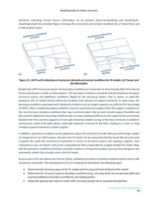


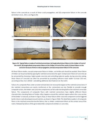

![Modelling Guide for Timber Structures
Floors and roofs- Chapter 6.1
31
primary geometric and material parameters are defined as follows: ℎ, depth; 𝐴𝐴, cross-sectional area; 𝐼𝐼,
moment of inertia; 𝐸𝐸, modulus of elasticity; 𝐿𝐿, span; and 𝑏𝑏, width of the cross-section of the concrete slab,
insulation, and timber with the subscript 𝑐𝑐, 𝑖𝑖𝑖𝑖, and 𝑡𝑡, respectively.
(a)
(b) (c)
Figure 26. TCC systemwith dowel-typemechanicalfasteners:(a)longitudinalsection; (b)cross-sectionwith
timber beam; and (c)cross-sectionwithMTP/SCL
(a) Effective Width, 𝑏𝑏𝑐𝑐
In the case of TCC with MTP at the bottom, the effective width, 𝑏𝑏𝑐𝑐, of the concrete slab equals the width of the
MTP and needs to be designed to a standard unit width. In the case of TCC with timber beams, the effective
width of the concrete slab may be based on the Canadian steel design standard CSA S16-14 (CSA Group,2014a).
This is considered to be conservative because of the lower composite action in TCC compared to steel-concrete
composite. The effective width of the concrete slab is calculated, based on Cuerrier-Auclair (2020), using
Equations 16 and 17 as follows:
𝒃𝒃𝒄𝒄,𝒆𝒆 = 𝐦𝐦𝐦𝐦𝐦𝐦(𝟎𝟎. 𝟏𝟏𝑳𝑳; 𝟏𝟏𝟏𝟏𝒉𝒉𝒄𝒄 ; 𝒃𝒃𝐞𝐞) [16]
𝒃𝒃𝒄𝒄,𝒊𝒊 = 𝐦𝐦𝐦𝐦𝐦𝐦(𝟎𝟎. 𝟐𝟐𝟐𝟐𝑳𝑳; 𝟐𝟐𝟐𝟐𝒉𝒉𝒄𝒄 ; 𝒃𝒃𝐦𝐦) [17]
where
𝑏𝑏𝑐𝑐,𝑒𝑒 = Effective width of an edge beam in mm
𝑏𝑏𝑐𝑐,𝑖𝑖 = Effective width of an internal beam in mm
𝐿𝐿 = Span of system in mm
ℎ𝑐𝑐 = Thicknessof the concrete slab in mm
𝑏𝑏𝑒𝑒 = The sum of the spacing between edge beam and internal beam, and half width of the edge
beam in mm
𝑏𝑏𝑚𝑚 = Actual spacing of the middle beams in mm](https://image.slidesharecdn.com/modellingguidefortimberstructures-240325073901-2a07d971/85/Modelling-Guide-for-Timber-Structures-FPInnovations-265-320.jpg)
![Modelling Guide for Timber Structures
Chapter 6.1 - Floors and roofs
32
The effective widths of concrete slabsin TCC with timber beams is illustrated in Figure 27.
Figure 27. Effectivewidth ofconcrete slab in TCC with timberbeams
(b) Effective Connector Spacing, 𝒔𝒔𝒆𝒆𝒆𝒆𝒆𝒆
For uniformly distributed connectors, the effective spacing is considered to be the actual spacing. For
nonuniformly distributed connectors, typical for a single-span TCC floor, the spacing is smaller at the end
quarters of the single-span beam and larger in the middle. The effective spacing, 𝑠𝑠𝑒𝑒𝑒𝑒𝑒𝑒 , of nonuniformly
distributed connectorscan be calculated as
𝒔𝒔𝒆𝒆𝒆𝒆𝒆𝒆 = 𝟎𝟎. 𝟕𝟕𝟕𝟕𝒔𝒔𝒎𝒎𝒎𝒎𝒎𝒎 + 𝟎𝟎. 𝟐𝟐𝟐𝟐𝒔𝒔𝒎𝒎𝒎𝒎𝒎𝒎 [18]
where
𝑠𝑠𝑚𝑚𝑚𝑚𝑚𝑚 = Minimum connector spacing,e.g., at the ends, in mm
𝑠𝑠𝑚𝑚𝑚𝑚𝑚𝑚 = Maximum connector spacing,e.g., in the middle of the beam, in mm
(c) Modulus of Elasticity of Concrete,𝑬𝑬𝒄𝒄
The modulus of elasticity of concrete,𝐸𝐸𝑐𝑐 , is an input parameter for the Gamma method. It can be determined
according to tests or standards. The following is an example for determining 𝐸𝐸𝑐𝑐 in accordance with the
Canadian concrete design standard, CSA-A23.3-14 (CSA Group, 2014b). The modulus of elasticity of normal
density concrete with compressive strength (𝑓𝑓
𝑐𝑐
′
) between 20 and 40 MPa can be calculated as
𝑬𝑬𝒄𝒄 = 𝟒𝟒𝟒𝟒𝟒𝟒𝟒𝟒�𝒇𝒇𝒄𝒄
′ [19]
For concrete density (𝜌𝜌𝑐𝑐 ) between 1500 and 2500 kg/m3, the modulus of elasticity accordingto CSA-A23.3-14
(CSA Group,2014b) can be calculated as
𝑬𝑬𝒄𝒄 = (𝟑𝟑𝟑𝟑𝟑𝟑𝟑𝟑�𝒇𝒇𝒄𝒄
′ + 𝟔𝟔𝟔𝟔𝟔𝟔𝟔𝟔)�
𝝆𝝆𝒄𝒄
𝟐𝟐𝟐𝟐𝟐𝟐𝟐𝟐
�
𝟏𝟏.𝟓𝟓
[20]
(d) Concrete Cracking
Concrete cracks that develop during curing as a result of shrinkage are usually controlled with the minimum
reinforcementspecified in codes.In the case of CSA-A23.3-14 (CSA Group, 2014b),for example, the minimum
reinforcementis 0.2% of the gross area of concrete. Cracks can also appear after the load is applied, with the
concrete starting to crack and the neutral axis moving towards the geometric centroid of the remaining cross-
section, where the cracked portion is neglected,resultingin a decrease in the bending stiffness of the system](https://image.slidesharecdn.com/modellingguidefortimberstructures-240325073901-2a07d971/85/Modelling-Guide-for-Timber-Structures-FPInnovations-266-320.jpg)
![Modelling Guide for Timber Structures
Floors and roofs- Chapter 6.1
33
and an increase in deflection (Mirdad, 2020).Cracking of concrete in the TCC system is important and should
be considered in the design. Cuerrier-Auclair et al. (2016b) present a moment-curvature method to account
for the influence of concrete cracking on the load-carrying capacity of a TCC beam. This method is based on a
1D FE analysis of the composite beam where the stiffness parametersof the concrete are updated ateach load
increment using a secant method by assuming a material law, that is, the stress-strain relationship, for the
concrete and the steel reinforcement.
More practical methods to account for the influence of concrete cracking are given in material design
standards, for example, CSA A23.3-14 (CSA Group, 2014b) and CSA S16-14 (CSA Group, 2014a). CSA A23.3-14
provides a simple empirical procedure to consider concrete cracking without reducing the concrete area by
excluding concrete in tension. For normal weight concrete, the steel standard CSA S16-14 neglects the
contribution of the tensile resistance of concrete when calculating the strength and stiffness of steel-concrete
composite beams. A similar approach can be used in TCC beam design. Accordingto CSA A23.3-14,the gross
moment of inertia (𝐼𝐼𝑔𝑔) of concrete is permitted in elastic analysis to check ultimate limit state designs. To
accountfor reduced capacity after concrete cracking,areduction factor of 0.35 isapplied to the gross moment
of inertia, as shown in Equation 21,
𝑰𝑰𝒄𝒄 = 𝟎𝟎. 𝟑𝟑𝟑𝟑𝑰𝑰𝒈𝒈 [21]
where
𝐼𝐼𝑐𝑐 = Reduced second moment of inertia of cracked concrete
𝐼𝐼𝑔𝑔 = Gross second moment of inertia of concrete
This factor was conservatively enforced by various standards to account for capacity loss due to concrete
cracking.A similar approach to accountfor concrete crackingcan be adopted for TCC systems.
(2) Maximum Stressesand Connection Forces
The maximum normal stressesin a TCC system can be calculated using Equation 2. Figure 28 shows the stress
distribution in a TCC system with beams. The shear stress in the wood-based panel or beams can be estimated
using Equation 3. The stress limit needsto be checked for timber and concrete resistance.
Figure 28. Stressdistributions of TCC system based on Gamma method](https://image.slidesharecdn.com/modellingguidefortimberstructures-240325073901-2a07d971/85/Modelling-Guide-for-Timber-Structures-FPInnovations-267-320.jpg)
![Modelling Guide for Timber Structures
Chapter 6.1 - Floors and roofs
34
Taking the Canadian concrete standard CSA A23.3-14 (CSA Group,2014b) asan example,the top extreme fibre
stress of concrete in compression must not be greater than its factored compressive strength, as follows:
𝝈𝝈𝒄𝒄,𝒄𝒄 ≤ 𝟎𝟎. 𝟗𝟗𝝓𝝓𝒄𝒄 𝒇𝒇𝒄𝒄
′
[22]
where
𝜎𝜎𝑐𝑐,𝑐𝑐 = Concrete compressive stressat the top in N/mm2
𝜙𝜙𝑐𝑐 = Resistance factor for concrete
𝑓𝑓
𝑐𝑐
′ = Specified compressive strength of concrete in N/mm2
No specific verification needsto be made for the concrete in tension because its contributions are neglected.
If the designer wants to minimise the concrete crackingin tension,the bottom extreme fibre stressof concrete
in tension can be limited to its factored modulus of rupture,as follows:
𝝈𝝈𝒄𝒄,𝒕𝒕 ≤ 𝝓𝝓𝒄𝒄 (𝟎𝟎.𝟔𝟔𝟔𝟔�𝒇𝒇𝒄𝒄
′ ) [23]
where
𝜎𝜎𝑐𝑐,𝑡𝑡 = Concrete tensile stress at bottom in N/mm2
𝜆𝜆 = Modification factor for concrete density accordingto CSA A23.3-14 (CSA Group,2014b)
Based on CSA A23.3-14, the resistance of the concrete needs to be checked to determine whether there is a
small tensile stress or full compressive stress in the concrete (CSA Group, 2014b). For the design load, it is
necessary to ensure that the concrete has sufficient compressive strength to avoid failure before the
connectorsfail, that is, that the compressive resistance of the concrete exceedsthe sum of shear forcesin all
the connectorsbetween the zero and the maximum bending moment locations.
The concrete resistance for each possible case is shown in Figure 29 and can be calculated as follows:
Case 1: The neutral axis is in the cross-section,𝑦𝑦𝑐𝑐 ≤ ℎ𝑐𝑐 , that is, a tensile stressis induced in the bottom portion:
𝑿𝑿𝒔𝒔𝒔𝒔𝒔𝒔 ≤ 𝜶𝜶𝟏𝟏𝜷𝜷𝟏𝟏𝒃𝒃𝒄𝒄 𝒚𝒚𝒄𝒄 𝒇𝒇𝒄𝒄
′
[24]
Case 2: The neutral axis is beyond the cross-section,𝑦𝑦𝑐𝑐 > ℎ𝑐𝑐 , that is, full compressive stress is induced in the
cross-section:
𝑿𝑿𝒔𝒔𝒔𝒔𝒔𝒔 ≤ 𝜶𝜶𝟏𝟏𝜷𝜷𝟏𝟏𝒃𝒃𝒄𝒄𝒉𝒉𝒄𝒄𝒇𝒇𝒄𝒄
′
[25]
where
ℎ𝑐𝑐 = Concrete thicknessin mm
𝑦𝑦𝑐𝑐 = Distance of the neutral axis of concrete to the compression edge in mm
=
ℎ𝑐𝑐 (𝜎𝜎𝑐𝑐,𝑁𝑁 + 𝜎𝜎𝑐𝑐,𝐵𝐵)
2𝜎𝜎𝑐𝑐,𝐵𝐵
with
𝜎𝜎𝑐𝑐,𝑁𝑁 = compressive stress in concrete induced by axial force in N/mm2
𝜎𝜎𝑐𝑐,𝐵𝐵 = tensile stress of concrete atbottom in N/mm2
𝛼𝛼1 = 0.85 − 0.0015𝑓𝑓
𝑐𝑐
′
𝛽𝛽1 = 0.97 − 0.0025𝑓𝑓
𝑐𝑐
′](https://image.slidesharecdn.com/modellingguidefortimberstructures-240325073901-2a07d971/85/Modelling-Guide-for-Timber-Structures-FPInnovations-268-320.jpg)
![Modelling Guide for Timber Structures
Floors and roofs- Chapter 6.1
35
𝑏𝑏𝑐𝑐 = Width of concrete in mm
𝑓𝑓𝑐𝑐
′
= Compressive strength of concrete in N/mm2
𝑋𝑋𝑠𝑠𝑠𝑠𝑠𝑠 = Sum of shear forcesin all the connectorsbetween the zero and the maximum bending
moment locations, in N
Figure 29. Stressdistributions in concrete
The shear load on a connector can be determined usingEquation 4. It should be smaller than the yield
capacity of the connector.
(3) Deflection
For mid- to large-span TCC systems, the short- and long-term deflections related to serviceability limit state
are usually the most critical principles.The short-term deflection of the TCC system can be estimated using the
standard beam equations, for example, Equation 5, with the effective bending stiffness calculated using
Equation 1 as input. In the extended service period of the system, long-term behaviour such as creep,
mechanosorptive creep,and shrinkage may occur; these will influence the internal forcesand stresses on the
components.
Shrinkage in concrete inducestensile stress in the concrete slab, which is usually balanced by compression in
the timber element. This tensile stress can propagate cracksin concrete,which reducesthe deflection due to
shrinkage. In the long term, the stress due to shrinkage can be relaxed due to the creep phenomena, which
also reducesthe deflection due to shrinkage. Accountingfor all these phenomena is complex and, to promote
this system with a more realistic implication, conservative creep adjustment factors can be applied for the
effective long-term modulus of each component by neglecting shrinkage. The long-term deflection due to
shrinkage of concrete can be reduced by shoring the TCC system before casting the concrete in the
prefabrication or on-site application (Fragiacomo & Lukaszewska, 2015).Accordingto Cuerrier-Auclair (2020),
the specified modulusof elasticity of the concrete,𝐸𝐸𝑐𝑐,𝐿𝐿𝐿𝐿 , modulus of elasticity of timber, 𝐸𝐸𝑡𝑡,𝐿𝐿𝐿𝐿 , and stiffness of
the shear connectors,𝑘𝑘𝐿𝐿𝐿𝐿 , may be multiplied by the creep adjustment factor for long-term load duration for
both serviceability and ultimate limit states, as follows:
𝑬𝑬𝒄𝒄,𝑳𝑳𝑳𝑳 = 𝟎𝟎. 𝟑𝟑𝟑𝟑𝑬𝑬𝒄𝒄 [26]
𝑬𝑬𝒕𝒕,𝑳𝑳𝑳𝑳 = 𝟎𝟎. 𝟓𝟓𝑬𝑬𝒕𝒕 [27]
𝒌𝒌𝑳𝑳𝑳𝑳 = 𝟎𝟎. 𝟐𝟐𝟐𝟐𝟐𝟐 [28]](https://image.slidesharecdn.com/modellingguidefortimberstructures-240325073901-2a07d971/85/Modelling-Guide-for-Timber-Structures-FPInnovations-269-320.jpg)
![Modelling Guide for Timber Structures
Chapter 6.1 - Floors and roofs
36
In the case of a soft insulation and thin timber planks, the bending stiffness, 𝐸𝐸𝑖𝑖𝑖𝑖 𝐼𝐼𝑖𝑖𝑖𝑖, is small compared with
those of concrete and timber and can be ignored in the design.
(4) Vibration
TCC floorsshould be evaluated to preventobjectionable vibrations.Accordingto Hu etal. (2016),the vibration-
controlled span of a TCC floor can be directly calculated using Equation 29:
𝑳𝑳 ≤ 𝟎𝟎.𝟑𝟑𝟑𝟑𝟑𝟑
((𝑬𝑬𝑬𝑬)𝒆𝒆𝒆𝒆𝒆𝒆
𝟏𝟏𝟏𝟏)𝟎𝟎.𝟐𝟐𝟐𝟐𝟐𝟐
�𝒎𝒎𝒂𝒂
𝟏𝟏𝟏𝟏�
𝟎𝟎.𝟐𝟐𝟐𝟐𝟐𝟐 [29]
where
(𝐸𝐸𝐸𝐸)𝑒𝑒𝑒𝑒𝑒𝑒
1𝑚𝑚 = Effective bending stiffness of a 1 m wide strip composite beam in N∙m2
𝑚𝑚𝑎𝑎
1𝑚𝑚 = Mass per unit length of a 1 m wide strip of TCC beam in kg/m
(5) Limitations of Gamma method for TCC systems
This simplified method is particularly accurate for predicting the structural performance of the composite
beams in which all materials remain linear-elastic (Yeoh, Fragiacomo, De Franceschi, & Heng Boon, 2011).
However,there are some limitations in the application:
• The shear forcesbetween timber and concrete are assumed to be uniformly transferred,which isvalid
for continuous connections such as adhesives, continuous HBV plates, and closely spaced STSs. The
connections must be uniformly stiff and equally spaced so that the connection stiffness can be
smeared along the beam axis. For widely spaced connections, this assumption could lead to
unacceptable errors.
• This method assumes a simply supported beam subjected to a sinusoidal distributed load with a
deflection also in a sinusoidal shape. For other supportingconditionsand load forms, this method may
yield predictionsthat are nonconservative.
• This method is based on the theory of linear elasticity; cracking of concrete and plasticity of
connectionsare therefore notconsidered.Van der Linden (1999) modified the Gamma method to the
frozen shear force model by considering,in part, the ductility of the connection.Once the applied load
approaches the elastic limit load, the connectors closest to the support yield first. At this point, the
model assumes the entire system has yielded. This approach significantly underestimates the load-
carryingcapacity of composite systems.
To overcome these limitations, discrete bond models (discussed in Section 6.1.3.2.2) can be suitable
alternatives.
6.1.3.2.2 Discrete Bond Models
6.1.3.2.2.1 Overview of Discrete Bond Models
For a composite floor with widely spaced connections, the components are only connected at discrete
locations. Using a continuous bond model may lead to unacceptable errors,and discrete bond models should](https://image.slidesharecdn.com/modellingguidefortimberstructures-240325073901-2a07d971/85/Modelling-Guide-for-Timber-Structures-FPInnovations-270-320.jpg)


![Modelling Guide for Timber Structures
Floors and roofs- Chapter 6.1
39
Under the external applied load, the connectorsnear the support will reach their yield strength first because
of the higher shear forces, given that all connectors are of the same type. Once the connectors near the
supports yield,the load will be redistributed to the remainingelastic connectorsuntil they also yield. A yielded
connector does not contribute to resisting a load greater than its yield load, which is the basis for an
incremental method to calculate the shear force in the concrete-timber connection.Asa result, the nonlinear
calculation for the connector force can be performed by combining the linear calculation with incremental
loading. The incremental loading and deflection can be calculated because of the load redistributions in the
system after each connector hasyielded.
(1) Effective Bending Stiffness, (EI)𝒆𝒆𝒆𝒆𝒆𝒆
The effective bending stiffness, (𝐸𝐸𝐸𝐸)𝑒𝑒𝑒𝑒𝑒𝑒 , of the TCC system can be directly calculated from the closed-form
solution shown in Equation 30.
(EI)𝒆𝒆𝒆𝒆𝒆𝒆 =
𝑳𝑳𝟒𝟒(𝑬𝑬𝒄𝒄𝑰𝑰𝒄𝒄+𝑬𝑬𝒕𝒕𝑰𝑰𝒕𝒕
)𝟐𝟐��
(𝑬𝑬𝒄𝒄𝑨𝑨𝒄𝒄+𝑬𝑬𝒕𝒕𝑨𝑨𝒕𝒕)
𝟐𝟐𝑬𝑬𝒄𝒄𝑨𝑨𝒄𝒄𝑬𝑬𝒕𝒕𝑨𝑨𝒕𝒕
+
𝑯𝑯𝟐𝟐−𝒉𝒉𝒊𝒊
𝟐𝟐
𝟖𝟖(𝑬𝑬𝒄𝒄𝑰𝑰𝒄𝒄+𝑬𝑬𝒕𝒕𝑰𝑰𝒕𝒕)
� ∑ 𝒏𝒏𝒊𝒊
𝒓𝒓
𝒊𝒊=𝟏𝟏 +𝟏𝟏
𝒌𝒌
� �
𝑳𝑳𝟒𝟒(𝑬𝑬𝒄𝒄𝑰𝑰𝒄𝒄+𝑬𝑬𝒕𝒕𝑰𝑰𝒕𝒕)��
(𝑬𝑬𝒄𝒄𝑨𝑨𝒄𝒄+𝑬𝑬𝒕𝒕𝑨𝑨𝒕𝒕)
𝟐𝟐𝑬𝑬𝒄𝒄𝑨𝑨𝒄𝒄𝑬𝑬𝒕𝒕𝑨𝑨𝒕𝒕
+
𝑯𝑯𝟐𝟐−𝒉𝒉𝒊𝒊𝒊𝒊
𝟐𝟐
𝟖𝟖(𝑬𝑬𝒄𝒄𝑰𝑰𝒄𝒄+𝑬𝑬𝒕𝒕𝑰𝑰𝒕𝒕)
� ∑ 𝒏𝒏𝒊𝒊
𝒓𝒓
𝒊𝒊=𝟏𝟏 +𝟏𝟏
𝒌𝒌
� �−𝟎𝟎.𝟎𝟎𝟎𝟎𝟎𝟎𝟎𝟎𝟎𝟎(𝑯𝑯+𝒉𝒉𝒊𝒊𝒊𝒊)(𝟐𝟐𝟐𝟐𝟐𝟐𝟏𝟏 −𝒏𝒏𝟏𝟏
𝟐𝟐
)�𝟑𝟑𝟑𝟑𝟐𝟐𝒏𝒏𝟏𝟏−𝒏𝒏𝟏𝟏
𝟑𝟑�
[30]
where
𝐸𝐸𝑐𝑐 = Modulus of elasticity of concrete in N/mm2
𝐸𝐸𝑡𝑡 = Modulus of elasticity of timber in N/mm2
𝐼𝐼𝑐𝑐 = Moment of inertia of concrete in mm4
𝐼𝐼𝑡𝑡 = Moment of inertia of timber in mm4
𝐴𝐴𝑐𝑐 = Cross-sectional area of concrete in mm2
𝐴𝐴𝑡𝑡 = Cross-sectional area of timber in mm2
𝐻𝐻 = Height of TCC section includingtimber, concrete,and insulation gap, in mm
ℎ𝑖𝑖𝑖𝑖 = Thicknessof insulation gap in mm
𝑛𝑛𝑖𝑖 = Distance of the connector frommid-span in mm
𝑛𝑛1 = Distance of the first connector frommid-span in mm
𝑟𝑟 = Number of connector rowsfrom mid-span to the support
𝑘𝑘 = Stiffness of the connector obtained from testing or from the analytical model, in N/mm
For timber-concrete joints with inclined mechanical connectors, for example, STSs, the analytical models
developed by Mirdad and Chui (2020a; 2020b) can be used to estimate the stiffness and strength. If the slip
modulus (ku) for ultimate limit states calculation is required,it can be assumed as two-thirds of the initial slip
modulus (European Committee for Standardization, 2004).
(2) Connector Forces
The effective force of the first outermost connector,𝐹𝐹𝑦𝑦,𝑒𝑒𝑒𝑒𝑒𝑒 , can be calculated as follows:
𝑭𝑭𝒚𝒚,𝒆𝒆𝒆𝒆𝒆𝒆 = 𝑿𝑿𝟏𝟏 =
𝒘𝒘𝒘𝒘�𝟑𝟑𝟑𝟑𝟐𝟐 𝒏𝒏𝟏𝟏−𝒏𝒏𝟏𝟏
𝟑𝟑�
𝟕𝟕𝟕𝟕.𝟖𝟖(𝑬𝑬𝒄𝒄𝑰𝑰𝒄𝒄+𝑬𝑬𝒕𝒕𝑰𝑰𝒕𝒕)��
(𝑬𝑬𝒄𝒄𝑨𝑨𝒄𝒄+𝑬𝑬𝒕𝒕𝑨𝑨𝒕𝒕)
𝟐𝟐𝑬𝑬𝒄𝒄𝑨𝑨𝒄𝒄𝑬𝑬𝒕𝒕𝑨𝑨𝒕𝒕
+
𝑯𝑯𝟐𝟐−𝒉𝒉𝒊𝒊𝒊𝒊
𝟐𝟐
𝟖𝟖(𝑬𝑬𝒄𝒄𝑰𝑰𝒄𝒄+𝑬𝑬𝒕𝒕𝑰𝑰𝒕𝒕)
� ∑ 𝒏𝒏𝒊𝒊
𝒓𝒓
𝒊𝒊=𝟏𝟏 +𝟏𝟏
𝒌𝒌
� �
[31]](https://image.slidesharecdn.com/modellingguidefortimberstructures-240325073901-2a07d971/85/Modelling-Guide-for-Timber-Structures-FPInnovations-273-320.jpg)
![Modelling Guide for Timber Structures
Chapter 6.1 - Floors and roofs
40
The sum of shear forces in all the connectors between the mid-span and a support, 𝑋𝑋𝑠𝑠𝑠𝑠𝑠𝑠 , is equal to the
resultant normal force at a given cross-section under applied load 𝑤𝑤. 𝑋𝑋𝑠𝑠𝑠𝑠𝑠𝑠 for a given load can be calculated
using the closed-formformula shown in Equation 32:
𝑿𝑿𝒔𝒔𝒔𝒔𝒔𝒔 = ∑ 𝑿𝑿𝒊𝒊
𝒓𝒓
𝒊𝒊=𝟏𝟏 =
𝒓𝒓𝒓𝒓𝒓𝒓�𝟑𝟑𝟑𝟑𝟐𝟐 𝒏𝒏𝟏𝟏−𝒏𝒏𝟏𝟏
𝟑𝟑�
𝟏𝟏𝟏𝟏𝟏𝟏(𝑬𝑬𝒄𝒄𝑰𝑰𝒄𝒄+𝑬𝑬𝒕𝒕𝑰𝑰𝒕𝒕)��
(𝑬𝑬𝒄𝒄𝑨𝑨𝒄𝒄+𝑬𝑬𝒕𝒕𝑨𝑨𝒕𝒕)
𝟐𝟐𝑬𝑬𝒄𝒄𝑨𝑨𝒄𝒄𝑬𝑬𝒕𝒕𝑨𝑨𝒕𝒕
+
𝑯𝑯𝟐𝟐−𝒉𝒉𝒊𝒊𝒊𝒊
𝟐𝟐
𝟖𝟖(𝑬𝑬𝒄𝒄𝑰𝑰𝒄𝒄+𝑬𝑬𝒕𝒕𝑰𝑰𝒕𝒕)
� ∑ 𝒏𝒏𝒊𝒊
𝒓𝒓
𝒊𝒊=𝟏𝟏 +𝟏𝟏
𝒌𝒌
� �
[32]
This sum of the shear forces, 𝑋𝑋𝑠𝑠𝑠𝑠𝑠𝑠 , is required to calculate the stresses in the TCC components and the
deflection under load, w.
(3) Maximum Stressesin Timber and Concrete
The stressesin concrete and timber under the applied load (e.g.,concrete compression,timber tension,and/or
shear) should be checked to determine if either fails before the yieldingof the first outermost connectors.As
illustrated in Figures31 and 32,the total stress at each position in a cross-section can be calculated by summing
the axial stress fromsubsystem 1 due to bendingand the axial stressfromsubsystem 2 due to the normal force
and bending.
Figure 31. Stressdistributionsin TCC systemswith masstimberbeamand concrete slab
Figure 32. Stressdistributionsin TCC systemswith MTP or SCL and concrete slabs](https://image.slidesharecdn.com/modellingguidefortimberstructures-240325073901-2a07d971/85/Modelling-Guide-for-Timber-Structures-FPInnovations-274-320.jpg)
![Modelling Guide for Timber Structures
Floors and roofs- Chapter 6.1
41
Accordingto the equilibriumcondition,the resultantnormal force applied in the timber and concrete atagiven
cross-section is equal to the sum of shear forces, 𝑋𝑋𝑠𝑠𝑠𝑠𝑠𝑠 , in all the connectors between the mid-span and
support. Therefore,the axial stress in the members is
𝝈𝝈𝒕𝒕,𝑵𝑵 =
𝑿𝑿𝒔𝒔𝒔𝒔𝒔𝒔
𝑨𝑨𝒕𝒕
[33]
𝝈𝝈𝒄𝒄,𝑵𝑵 =
𝑿𝑿𝒔𝒔𝒔𝒔𝒔𝒔
𝑨𝑨𝒄𝒄
[34]
where
𝜎𝜎𝑡𝑡,𝑁𝑁 = Tensile stress in timber induced by axial forces in N/mm2
The resultant axial stress due to bending at a position in the cross-section is the sum of the bending stresses
obtained from the two subsystems, as shown below:
𝝈𝝈𝒕𝒕,𝑩𝑩 = 𝝈𝝈𝟏𝟏,𝒕𝒕 + 𝝈𝝈𝟐𝟐,𝒕𝒕 [35]
𝝈𝝈𝒄𝒄,𝑩𝑩 = 𝝈𝝈𝟏𝟏,𝒄𝒄 + 𝝈𝝈𝟐𝟐,𝒄𝒄 [36]
where
𝜎𝜎𝑡𝑡,𝐵𝐵 = Normal stress in timber induced by bendingmoment in timber
𝜎𝜎𝑐𝑐,𝐵𝐵 = Normal stress in concrete induced by bendingmoment in concrete
𝜎𝜎𝑖𝑖,𝑡𝑡 = Bending stressin timber in subsystem i in N/mm2
𝜎𝜎𝑖𝑖,𝑐𝑐 = Bending stressin concrete in subsystem i in N/mm2
In subsystem 1, the normal stress in the member is caused by the bendingmoment assuming the concrete and
timber are unconnected,while in subsystem 2, the normal stress iscaused by the bendingmoment induced by
the eccentric normal force.The stresses can be written as follows,
𝝈𝝈𝟏𝟏,𝒕𝒕 =
𝟑𝟑𝟑𝟑∙𝑬𝑬𝒕𝒕𝑰𝑰𝒕𝒕�𝑳𝑳𝟐𝟐−𝒏𝒏𝒊𝒊
𝟐𝟐�
𝟒𝟒𝒃𝒃𝒕𝒕𝒉𝒉𝒕𝒕
𝟐𝟐(𝑬𝑬𝒄𝒄𝑰𝑰𝒄𝒄+𝑬𝑬𝒕𝒕𝑰𝑰𝒕𝒕)
[37]
𝝈𝝈𝟏𝟏,𝒄𝒄 =
𝟑𝟑𝟑𝟑∙𝑬𝑬𝒄𝒄𝑰𝑰𝒄𝒄�𝑳𝑳𝟐𝟐−𝒏𝒏𝒊𝒊
𝟐𝟐�
𝟒𝟒𝒃𝒃𝒄𝒄𝒉𝒉𝒄𝒄
𝟐𝟐(𝑬𝑬𝒄𝒄𝑰𝑰𝒄𝒄+𝑬𝑬𝒕𝒕𝑰𝑰𝒕𝒕)
[38]
𝝈𝝈𝟐𝟐,𝒕𝒕 =
𝟑𝟑𝟑𝟑𝒔𝒔𝒔𝒔𝒔𝒔𝑬𝑬𝒕𝒕𝑰𝑰𝒕𝒕(𝑯𝑯+𝒉𝒉𝒊𝒊𝒊𝒊)
𝒃𝒃𝒕𝒕𝒉𝒉𝒕𝒕
𝟐𝟐
(𝑬𝑬𝒄𝒄𝑰𝑰𝒄𝒄+𝑬𝑬𝒕𝒕𝑰𝑰𝒕𝒕)
[39]
𝝈𝝈𝟐𝟐,𝒄𝒄 =
𝟑𝟑𝟑𝟑𝒔𝒔𝒔𝒔𝒔𝒔𝑬𝑬𝒄𝒄𝑰𝑰𝒄𝒄(𝑯𝑯+𝒉𝒉𝒊𝒊𝒊𝒊)
𝒃𝒃𝒄𝒄𝒉𝒉𝒄𝒄
𝟐𝟐(𝑬𝑬𝒄𝒄𝑰𝑰𝒄𝒄+𝑬𝑬𝒕𝒕𝑰𝑰𝒕𝒕)
[40]
The total axial stress for the member is the sum of the stressesin the subsystems and can be written as
𝝈𝝈𝒕𝒕,𝒛𝒛 = 𝝈𝝈𝒕𝒕,𝑵𝑵 + 𝝈𝝈𝒕𝒕,𝑩𝑩 [41]
𝝈𝝈𝒄𝒄,𝒛𝒛 = 𝝈𝝈𝒄𝒄,𝑵𝑵 + 𝝈𝝈𝒄𝒄,𝑩𝑩 [42]
where
𝜎𝜎𝑡𝑡,𝑧𝑧 = Total tensile stress 𝜎𝜎𝑡𝑡,𝑡𝑡 or total compressive stress𝜎𝜎𝑡𝑡,𝑐𝑐 of timber in N/mm2
𝜎𝜎𝑐𝑐,𝑧𝑧 = Total tensile stress 𝜎𝜎𝑐𝑐,𝑡𝑡 or total compressive stress𝜎𝜎𝑐𝑐,𝑐𝑐 of concrete in N/mm2](https://image.slidesharecdn.com/modellingguidefortimberstructures-240325073901-2a07d971/85/Modelling-Guide-for-Timber-Structures-FPInnovations-275-320.jpg)
![Modelling Guide for Timber Structures
Chapter 6.1 - Floors and roofs
42
The shear stress is most critical in the timber member, and the maximum stress happensat the neutral axis of
the timber member where flexural stress is zero. The shear stress of timber, 𝜏𝜏𝑡𝑡, can be calculated using the
neutral axis of timber, as shown in Equation 43:
𝝉𝝉𝒕𝒕 =
𝒉𝒉𝒕𝒕
𝟐𝟐
(𝝈𝝈𝒕𝒕,𝑵𝑵+𝝈𝝈𝒕𝒕,𝑩𝑩)𝟐𝟐𝑬𝑬𝒕𝒕𝑽𝑽
𝟖𝟖𝝈𝝈𝒕𝒕,𝑩𝑩
𝟐𝟐
(𝑬𝑬𝑬𝑬)𝒆𝒆𝒆𝒆𝒆𝒆
[43]
where
ℎ𝑡𝑡 = Height of timber in mm
𝑉𝑉 = Shear force in the composite cross-section of interestin N
Note that the neutral axes move further apart from each other and towards the centroid of each member as
the degree of composite action decreases.
The superposition method can also be applied to mass timber floors. The stress distribution of a ribbed-plate
system is shown in Figure 33.In the case of a ribbed-plate system with timber beams and MTP, the stressesin
the MTP as well as the timber beams need to be checked separately.
Figure 33. Stressdistributionsin compositesystemswith masstimber beamsand MTP or SCL
(4) Deflection,∆
The vertical deflection of the TCC system under a uniformly distributed load, 𝑤𝑤, can be calculated using
Equation 44:
∆=
𝟓𝟓𝟓𝟓𝑳𝑳𝟒𝟒−𝟏𝟏𝟏𝟏.𝟐𝟐𝑿𝑿𝒔𝒔𝒔𝒔𝒔𝒔𝒏𝒏𝟏𝟏(𝟐𝟐𝟐𝟐−𝒏𝒏𝒓𝒓)(𝑯𝑯+𝒉𝒉𝒊𝒊𝒊𝒊)
𝟑𝟑𝟑𝟑𝟑𝟑(𝑬𝑬𝒄𝒄𝑰𝑰𝒄𝒄+𝑬𝑬𝒕𝒕𝑰𝑰𝒕𝒕)
[44]
To calculate the long-term deflection,the modulus of elasticity of the concrete (𝐸𝐸𝑐𝑐 ,𝐿𝐿𝐿𝐿 ),modulus of elasticity of
timber (𝐸𝐸𝑡𝑡,𝐿𝐿𝐿𝐿 ), and stiffness of the shear connectors (𝑘𝑘𝐿𝐿𝐿𝐿 ) may be multiplied by the creep adjustment factors
for long-term load duration for both serviceability and ultimate limit states, as given in Equations 26 to 28.
(5) Vibration
TCC floors should be evaluated to preventobjectionable vibrations, as shown in Equation 29. An example of a
TCC floor system with an MTP is shown in Appendix B.](https://image.slidesharecdn.com/modellingguidefortimberstructures-240325073901-2a07d971/85/Modelling-Guide-for-Timber-Structures-FPInnovations-276-320.jpg)


![Modelling Guide for Timber Structures
Floors and roofs- Chapter 6.1
45
This release-and-restore method was conducted using the matrix method. Presented beloware the governing
equations and solution for a TCC beam with simple supports, as illustrated in Figure 34. For supportconditions
other than the simple support, see Zhang, Zhang and Chui (2021).
The unknown slip vectorsare
{𝑺𝑺𝟏𝟏
} = [𝒔𝒔𝟏𝟏𝟏𝟏, 𝒔𝒔𝟐𝟐𝟐𝟐, 𝒔𝒔𝟑𝟑𝟑𝟑, … , 𝒔𝒔𝒏𝒏𝒏𝒏
]𝑻𝑻
[45]
{𝑺𝑺𝟐𝟐
} = [𝒔𝒔𝟏𝟏𝟏𝟏, 𝒔𝒔𝟐𝟐𝟐𝟐, 𝒔𝒔𝟑𝟑𝟑𝟑, … , 𝒔𝒔𝒏𝒏𝒏𝒏
]𝑻𝑻
[46]
{𝑫𝑫} = [𝒅𝒅𝟏𝟏, 𝒅𝒅𝟐𝟐 , 𝒅𝒅𝟑𝟑, … , 𝒅𝒅𝒏𝒏
]𝑻𝑻
[47]
Under the simple support conditions, the slip vector {S1} can be solved and expressed as
{𝑺𝑺𝟏𝟏
} = [(𝑾𝑾𝟐𝟐 − 𝑾𝑾𝟏𝟏
) + (𝑾𝑾𝟏𝟏 + 𝑾𝑾𝟐𝟐
)(𝟐𝟐𝟐𝟐 + 𝜣𝜣𝜣𝜣)−𝟏𝟏
𝜣𝜣𝜣𝜣]−𝟏𝟏
𝑾𝑾𝟐𝟐
{𝜦𝜦} [48]
where 𝐼𝐼 is the identity matrix
𝑰𝑰 =
⎣
⎢
⎢
⎢
⎡
𝟏𝟏
𝟏𝟏
𝟏𝟏
⋱
𝟏𝟏 ⎦
⎥
⎥
⎥
⎤
𝒏𝒏×𝒏𝒏
[49]
Vector {𝛬𝛬} is
{𝜦𝜦} = [𝝀𝝀𝟏𝟏, 𝝀𝝀𝟐𝟐, 𝝀𝝀𝟑𝟑 , … , 𝝀𝝀𝒏𝒏
]𝑻𝑻
[50]
in which 𝜆𝜆𝑖𝑖, the difference of length change between the bottom of the concrete and the top of timber in the
released segment,
𝝀𝝀𝒊𝒊 =
(𝒉𝒉𝒄𝒄+𝒉𝒉𝒕𝒕)
𝟐𝟐(𝑬𝑬𝒄𝒄𝑰𝑰𝒄𝒄+𝑬𝑬𝒕𝒕𝑰𝑰𝒕𝒕)
𝒍𝒍𝒊𝒊𝑴𝑴
�𝒊𝒊 [51]
and 𝑀𝑀
�𝑖𝑖 is the average external bendingmoment in segment 𝑖𝑖
𝑴𝑴
�𝒊𝒊 =
𝟏𝟏
𝒍𝒍𝒊𝒊
∫ 𝑴𝑴(𝒙𝒙)𝒅𝒅𝒅𝒅
𝒙𝒙𝒊𝒊+𝒍𝒍𝒊𝒊
𝒙𝒙𝒊𝒊
[52]
Matrix 𝛩𝛩 is the parameter matrix
𝜣𝜣 =
⎣
⎢
⎢
⎢
⎡
𝜽𝜽𝟏𝟏
𝜽𝜽𝟐𝟐
𝜽𝜽𝟑𝟑
⋱
𝜽𝜽𝒏𝒏⎦
⎥
⎥
⎥
⎤
𝒏𝒏×𝒏𝒏
[53]
in which
𝜽𝜽𝒊𝒊 =
𝒍𝒍𝒊𝒊
𝑬𝑬𝒕𝒕
�
�
𝒉𝒉𝒕𝒕
𝟐𝟐
+𝒆𝒆�𝒉𝒉𝒕𝒕
𝟐𝟐𝑰𝑰𝒕𝒕
+
𝟏𝟏
𝑨𝑨𝒕𝒕
� +
𝒍𝒍𝒊𝒊
𝑬𝑬𝒄𝒄
�
�
𝒉𝒉𝒄𝒄
𝟐𝟐
+𝒆𝒆�𝒉𝒉𝒄𝒄
𝟐𝟐𝑰𝑰𝒄𝒄
+
𝟏𝟏
𝑨𝑨𝒄𝒄
� [54]](https://image.slidesharecdn.com/modellingguidefortimberstructures-240325073901-2a07d971/85/Modelling-Guide-for-Timber-Structures-FPInnovations-279-320.jpg)
![Modelling Guide for Timber Structures
Chapter 6.1 - Floors and roofs
46
and 𝑒𝑒 is the eccentricity of axial forcesin the restored segment
𝒆𝒆 =
𝑬𝑬𝒕𝒕𝑰𝑰𝒕𝒕𝒉𝒉𝒄𝒄−𝑬𝑬𝒄𝒄𝑰𝑰𝒄𝒄𝒉𝒉𝒕𝒕
𝟐𝟐(𝑬𝑬𝒄𝒄𝑰𝑰𝒄𝒄+𝑬𝑬𝒕𝒕𝑰𝑰𝒕𝒕)
[55]
The stiffness matrix 𝐾𝐾 can be expressed as
𝑲𝑲 =
⎣
⎢
⎢
⎢
⎡
𝒌𝒌𝟏𝟏
𝒌𝒌𝟏𝟏
𝒌𝒌𝟏𝟏
⋮
𝒌𝒌𝟏𝟏
𝒌𝒌𝟐𝟐
𝒌𝒌𝟐𝟐
⋮
𝒌𝒌𝟐𝟐
𝒌𝒌𝟑𝟑
⋮
𝒌𝒌𝟑𝟑
⋱
⋯ 𝒌𝒌𝒏𝒏⎦
⎥
⎥
⎥
⎤
𝒏𝒏×𝒏𝒏
[56]
Matrices 𝑊𝑊1 and 𝑊𝑊2 are expressed as
𝑾𝑾𝟏𝟏 =
⎣
⎢
⎢
⎢
⎡
𝟎𝟎
𝟎𝟎
⋮
𝟎𝟎
𝒌𝒌𝟏𝟏
𝟏𝟏
𝟎𝟎
⋮
𝟎𝟎
𝒌𝒌𝟐𝟐
𝟎𝟎
𝟏𝟏
⋮
𝟎𝟎
𝒌𝒌𝟑𝟑
⋯
⋯
⋱
⋯
⋯
𝟎𝟎
𝟎𝟎
⋮
𝟏𝟏
𝒌𝒌𝒏𝒏⎦
⎥
⎥
⎥
⎤
𝒏𝒏×𝒏𝒏
[57]
𝑾𝑾𝟐𝟐 =
⎣
⎢
⎢
⎢
⎡
𝟏𝟏
𝟏𝟏
⋱
𝟏𝟏
−𝒌𝒌𝒏𝒏−𝟏𝟏⎦
⎥
⎥
⎥
⎤
𝒏𝒏×𝒏𝒏
[58]
The slip vectors{𝑆𝑆2
} and {𝐷𝐷} can be determined from
{𝑺𝑺𝟐𝟐
} = {𝜦𝜦} − {𝑺𝑺𝟏𝟏
} [59]
{𝑫𝑫} = (𝟐𝟐𝟐𝟐 + 𝜣𝜣𝜣𝜣)−𝟏𝟏
𝜣𝜣𝜣𝜣{𝑺𝑺𝟏𝟏
} [60]
The axial forcesin each segment can be determined from
{𝑵𝑵} = [𝑵𝑵𝟏𝟏, 𝑵𝑵𝟐𝟐, 𝑵𝑵𝟑𝟑, … , 𝑵𝑵𝒏𝒏
]𝑻𝑻
= 𝟐𝟐𝜣𝜣−𝟏𝟏{𝑫𝑫} [61]
The bendingmoments in the timber and concrete in each segment are given as
𝑴𝑴𝒄𝒄
(𝒙𝒙) =
𝑬𝑬𝒄𝒄𝑰𝑰𝒄𝒄
𝑬𝑬𝒄𝒄𝑰𝑰𝒄𝒄+𝑬𝑬𝒕𝒕𝑰𝑰𝒕𝒕
𝑴𝑴(𝒙𝒙) − 𝑵𝑵𝒊𝒊 �
𝒉𝒉𝒄𝒄
𝟐𝟐
− 𝒆𝒆� [62]
𝑴𝑴𝒕𝒕
(𝒙𝒙) =
𝑬𝑬𝒕𝒕𝑰𝑰𝒕𝒕
𝑬𝑬𝒄𝒄𝑰𝑰𝒄𝒄+𝑬𝑬𝒕𝒕𝑰𝑰𝒕𝒕
𝑴𝑴(𝒙𝒙) − 𝑵𝑵𝒊𝒊 �
𝒉𝒉𝒕𝒕
𝟐𝟐
− 𝒆𝒆� [63]
The shear forcesin the timber and concrete can be stated as
𝑽𝑽𝒄𝒄
(𝒙𝒙) =
𝑬𝑬𝒄𝒄𝑰𝑰𝒄𝒄
𝑬𝑬𝒄𝒄𝑰𝑰𝒄𝒄+𝑬𝑬𝒕𝒕𝑰𝑰𝒕𝒕
𝑽𝑽(𝒙𝒙) [64]
𝑽𝑽𝒕𝒕
(𝒙𝒙) =
𝑬𝑬𝒕𝒕𝑰𝑰𝒕𝒕
𝑬𝑬𝒄𝒄𝑰𝑰𝒄𝒄+𝑬𝑬𝒕𝒕𝑰𝑰𝒕𝒕
𝑽𝑽(𝒙𝒙) [65]](https://image.slidesharecdn.com/modellingguidefortimberstructures-240325073901-2a07d971/85/Modelling-Guide-for-Timber-Structures-FPInnovations-280-320.jpg)
![Modelling Guide for Timber Structures
Floors and roofs- Chapter 6.1
47
Stressesat the top and bottom of the concrete are
𝜎𝜎𝑐𝑐,𝑐𝑐
(𝒙𝒙) = −
𝑬𝑬𝒄𝒄𝒉𝒉𝒄𝒄𝑴𝑴(𝒙𝒙)
𝟐𝟐(𝑬𝑬𝒄𝒄𝑰𝑰𝒄𝒄+𝑬𝑬𝒕𝒕𝑰𝑰𝒕𝒕)
+
𝑵𝑵𝒊𝒊�
𝒉𝒉𝒄𝒄
𝟐𝟐
−𝒆𝒆�𝒉𝒉𝒄𝒄
𝟐𝟐𝑰𝑰𝒄𝒄
−
𝑵𝑵𝒊𝒊
𝑨𝑨𝒄𝒄
[66]
𝜎𝜎𝑐𝑐,𝑡𝑡
(𝒙𝒙) =
𝑬𝑬𝒄𝒄𝒉𝒉𝒄𝒄𝑴𝑴(𝒙𝒙)
𝟐𝟐(𝑬𝑬𝒄𝒄𝑰𝑰𝒄𝒄+𝑬𝑬𝒕𝒕𝑰𝑰𝒕𝒕
)
−
𝑵𝑵𝒊𝒊�
𝒉𝒉𝒄𝒄
𝟐𝟐
−𝒆𝒆�𝒉𝒉𝒄𝒄
𝟐𝟐𝑰𝑰𝒄𝒄
−
𝑵𝑵𝒊𝒊
𝑨𝑨𝒄𝒄
[67]
Stressesat the top and bottom of the timber are
𝜎𝜎𝑡𝑡,𝑐𝑐
(𝒙𝒙) = −
𝑬𝑬𝒕𝒕𝒉𝒉𝒕𝒕𝑴𝑴(𝒙𝒙)
𝟐𝟐(𝑬𝑬𝒄𝒄𝑰𝑰𝒄𝒄+𝑬𝑬𝒕𝒕𝑰𝑰𝒕𝒕)
+
𝑵𝑵𝒊𝒊�
𝒉𝒉𝒕𝒕
𝟐𝟐
−𝒆𝒆�𝒉𝒉𝒕𝒕
𝟐𝟐𝑰𝑰𝒕𝒕
+
𝑵𝑵𝒊𝒊
𝑨𝑨𝒕𝒕
[68]
𝜎𝜎𝑡𝑡,𝑡𝑡
(𝒙𝒙) =
𝑬𝑬𝒕𝒕𝒉𝒉𝒕𝒕𝑴𝑴(𝒙𝒙)
𝟐𝟐(𝑬𝑬𝒄𝒄𝑰𝑰𝒄𝒄+𝑬𝑬𝒕𝒕𝑰𝑰𝒕𝒕)
−
𝑵𝑵𝒊𝒊�
𝒉𝒉𝒕𝒕
𝟐𝟐
−𝒆𝒆�𝒉𝒉𝒕𝒕
𝟐𝟐𝑰𝑰𝒕𝒕
+
𝑵𝑵𝒊𝒊
𝑨𝑨𝒕𝒕
[69]
The deflection of the beam can be determined using the Mohr integral method
∆(𝒕𝒕) = ∫
𝑴𝑴
�(𝒙𝒙,𝒕𝒕)𝑴𝑴𝒕𝒕𝒕𝒕𝒕𝒕(𝒙𝒙)
𝑬𝑬𝒄𝒄𝑰𝑰𝒄𝒄+𝑬𝑬𝒕𝒕𝑰𝑰𝒕𝒕
𝒅𝒅𝒅𝒅
𝑳𝑳
𝟎𝟎 [70]
where 𝑀𝑀
�(𝑥𝑥, 𝑡𝑡) is the moment distribution when a unit force is acting at the position of 𝑥𝑥 = 𝑡𝑡, and 𝑀𝑀𝑡𝑡𝑡𝑡𝑡𝑡(𝑥𝑥) is
the sum of moments in timber and concrete under the external load. The sum of moments in timber and
concrete is
𝑴𝑴𝒕𝒕𝒕𝒕𝒕𝒕(𝒙𝒙) = 𝑴𝑴(𝒙𝒙) −
(𝒉𝒉𝒄𝒄+𝒉𝒉𝒕𝒕)
𝟐𝟐
𝑵𝑵(𝒙𝒙) [71]
6.1.3.3 Numerical Methods
6.1.3.3.1 General Rules
While most TCC and mass timber floor systems can be analysed using the analytical methods described in
Section 6.1.3.2, advanced modellingmethods such as FE models can be used for casesbeyond the scope of the
analytical methods and the system development and optimisation. The modelling guidelines discussed in
Section 6.1.2.3, for light wood-frame systems, apply to the numerical modelling of TCC and mass timber floor
systems. In addition, the following additional guidelines are applicable:
• Adoptappropriate or equivalentmaterial propertiesfor concrete and timber based on experimentsor
appropriate literature, and accountfor concrete crackingin the material model.
• Consider the orthotropic nature of timber and the constitutive model to describe the nonlinear
behaviour.See, for example, WoodS (Chen et al., 2011) or WoodST (Chen et al., 2020).
• Model shear connectorsusingthe smeared or discrete contactelements,dependingon the connection
type and the layout of shear connectors.
• Adopt appropriate connection properties (load-slip response) based on experimental results or
modelling (for example, Mirdad & Chui, 2019).
Several researchershave conducted FEmodelling of TCC floor systems to evaluate their behaviour under out-
of-plane load (Fragiacomo, 2005; Fragiacomo & Ceccotti,2006; Fragiacomo etal., 2014; Gutkowski etal., 2010;
Khorsandnia etal., 2014; Liu,2016; Lopesetal., 2012; Lukaszewskaet al., 2010; Persaud & Symons, 2006; Van](https://image.slidesharecdn.com/modellingguidefortimberstructures-240325073901-2a07d971/85/Modelling-Guide-for-Timber-Structures-FPInnovations-281-320.jpg)

![Modelling Guide for Timber Structures
Floors and roofs- Chapter 6.1
49
Figure 36. Frameworkmodel
The shear connections are represented by hinged cantilevers that are rigidly connected to the timber and
concrete. The shear stiffness of the original connection is mimicked by adjusting the bending stiffness of the
cantilevers.As shown in Figure 37, the bending stiffness of cantileverscan be determined from:
(𝑬𝑬𝑬𝑬)𝒄𝒄𝒄𝒄𝒄𝒄𝒄𝒄𝒄𝒄𝒄𝒄𝒄𝒄𝒄𝒄𝒄𝒄𝒄𝒄 =
𝒌𝒌
𝟑𝟑
(𝒆𝒆𝟏𝟏
𝟑𝟑
+ 𝒆𝒆𝟐𝟐
𝟑𝟑) [72]
where
Figure 37. Shearconnection representedbyhinged cantileversin the frameworkmodel
Closely spaced shortstruts need to be builtin the framework model to connecttimber and concrete and ensure
the same vertical displacement of the two layers. The struts should be modelled as rigid bars that cannot
deformunder the vertical (axial) load.
6.1.3.3.3 Space-Exact Element Model
Nguyen et al. (2010; 2011) proposed an exact FE model for the linear static analysis of two-layer beams with
an interlayer slip. The layers are connected discontinuously and therefore the shear connections are modelled
using concentrated spring elements at each connector location (Figure 38[a]). It is assumed that no uplift can
occur at the top layer. Thus, both layers have the same transversal deflection but different rotations and
curvatures. The effect of friction at the interface is accounted for by assuming that the friction force is
proportional to the normal force at the interface. Based on these key assumptions, the governing equations
are established and an original closed-form solution is derived. From the analytical expressions for the
displacement and force fields, the space-exact stiffness matrix (Figure 38[b]) for a generic two-layer beam
element can be deduced and incorporated into any displacement-based FE code for the linear static analysis
(𝐸𝐸𝐸𝐸)𝑐𝑐𝑐𝑐𝑐𝑐𝑐𝑐𝑐𝑐𝑐𝑐𝑐𝑐𝑐𝑐𝑐𝑐𝑐𝑐 = Bending stiffness of the cantilever
𝑘𝑘 = Shear stiffness of the original connection
𝑒𝑒1 = Distance between the centroid of concrete to the joint
𝑒𝑒2 = Distance between the centroid of timber to the joint](https://image.slidesharecdn.com/modellingguidefortimberstructures-240325073901-2a07d971/85/Modelling-Guide-for-Timber-Structures-FPInnovations-283-320.jpg)


![Modelling Guide for Timber Structures
Floors and roofs- Chapter 6.1
57
6.1.7 References
Bedon,C., & Fragiacomo,M. (2017).Three-dimensional modellingof notched connectionsfor timber–concrete
composite beams. Structural Engineering International, 27(2), 184-196.
https://doi.org/10.2749/101686617X14881932435295
Berardinucci, B., Di Nino, S., Gregori, A., & Fragiacomo, M. (2017). Mechanical behavior of timber–concrete
connectionswith inclined screws. International Journal of Computational Methods and Experimental
Measurements, 5(6), 807-820.https://doi.org/10.2495/CMEM-V5-N6-807-820
Boccadoro, L., & Frangi, A. (2014). Experimental analysis of the structural behavior of timber-concrete
composite slabs made of beech-laminated veneer lumber. Journal of Performance of Constructed
Facilities, 28(6),A4014006.https://doi.org/10.1061/(ASCE)CF.1943-5509.0000552
Boccadoro, L., Zweidler, S., Steiger, R., & Frangi, A. (2017). Bending tests on timber-concrete composite
members made of beech laminated veneer lumber with notched connection.Engineering Structures,
132,14-28.https://doi.org/10.1016/j.engstruct.2016.11.029
Bocquet, J. F., Pizzi, A., & Resch,L. (2007).Full-scale industrial wood floor assembly and structuresby welded-
through dowels.HolzalsRoh- undWerkstoff,65(2),149-155.https://doi.org/10.1007/s00107-006-0170-4
Byfield,M. P. (2002).Analysisof composite beam with widely spaced shear connectors. Structural Engineering,
80(13):31-3.
CSA Group.(2014a). CSA S16-14: Design of steel structures. CSA Group.
CSA Group.(2014b).CSA-A23.3-14: Design of concrete structures. CSA Group.
CSA Group.(2019).CSA O86:19: Engineering design in wood. CSA Group.
Ceccotti, A. (2002). Composite concrete-timber structures. Progress in Structural Engineering and Materials,
2002(4),264-275.https://doi.org/10.1002/pse.126
Chen, Z., Zhu, E., & Pan, J. (2011). Numerical simulation of wood mechanical properties under complex state
of stress. Chinese Journal of Computational Mechanics, 28(04),629-634,640.
Chen,Z., Ni, C., Dagenais, C., & Kuan,S. (2020).WoodST: A temperature-dependentplastic-damage constitutive
model used for numerical simulation of wood-based materials and connections. Journal of Structural
Engineering, 146(3): A04019225.https://doi.org/10.1061/(ASCE)ST.1943-541X.0002524
Chui, Y. H. (2002). Application of ribbed-plate theory to predict vibrational serviceability of timber floor
systems. In Majid, W., M., W., A., Ahmad, Z., & Malik, A., R., A (Eds.), Proceedings of 7th World
Conference on Timber Engineering, WCTE 2002.
Cuerrier-Auclair, S. (2020). Design guide for timber-concrete composite floors in Canada. Special Publication
SP-540E.FPInnovations.
Cuerrier-Auclair, S., Sorelli, L., & Salenikovich, A. (2016a). A new composite connector for timber-concrete
composite structures. Construction and Building Materials, 112, 84-92.
https://doi.org/10.1016/j.conbuildmat.2016.02.025
Cuerrier-Auclair, S., Sorelli, L., & Salenikovich, A. (2016b). Simplified nonlinear model for timber-concrete
composite beams. International Journal of Mechanical Sciences, 117, 30-42.
https://doi.org/10.1016/j.ijmecsci.2016.07.019
Dassault Systèmes. (2019).Abaqus 2020.[Computer software].
Deam, B. L.,Fragiacomo,M., & Buchanan,A.H. (2008).Connectionsforcomposite concreteslab and LVL flooring
systems. Materials and Structures, 41(3),495-507.https://doi.org/10.1617/s11527-007-9261-x
DeutschesInstitut für Normung e. V. (2008).DIN 1052:2008-12: Design of timber structures - General rules and
rules for buildings.DIN DeutschesInstitut für Normung e. V.](https://image.slidesharecdn.com/modellingguidefortimberstructures-240325073901-2a07d971/85/Modelling-Guide-for-Timber-Structures-FPInnovations-291-320.jpg)

![Modelling Guide for Timber Structures
Floors and roofs- Chapter 6.1
59
Fridley, K. J., Rosowsky, D. V., & Hong, P. (1998). Time-dependent service-load behavior of wood floors:
Analytical model. Computers & Structures, 66(6), 847-860.https://doi.org/10.1016/S0045-
7949(97)00074-6
Gerber,A. R. (2016).Timber-concrete composite connectors in flat-plate engineered wood products. [Master’s
thesis, University of British Columbia]. https://doi.org/10.14288/1.0300229
Grosse, M., Hartnack, R., Lehmann, S., & Rautenstrauch, K. (2003). Modellierung von diskontinuierlich
verbundenen Holz-Beton-Verbundkonstruktionen / Teil 1: Kurzzeittragverhalten [Modelling of
discontinuously connected wood-concrete composite structures / Part 1: Short-term load-bearing
behavior].Bautechnik, 80(8),534-541.https://doi.org/10.1002/bate.200304120
Grosse, M., Hartnack, R., & Rautenstrauch, K. (2003). Modellierung von diskontinuierlich verbundenen Holz-
Beton-Verbunddecken / Teil 2: Langzeittragverhalten [Modellingof discontinuously connected wood-
concrete composite structures / Part 1: Long-term load-bearing behavior]. Bautechnik, 80(10), 693-
701.https://doi.org/10.1002/bate.200305110
Gutkowski, R. M., Balogh, J., & To, L. G. (2010). Finite-element modeling of short-term field response of
composite wood-concrete floors/decks. Journal of Structural Engineering, 136(6), 707-714.
https://doi.org/10.1061/(ASCE)ST.1943-541X.0000117
Gutkowski, R. M., Brown, K., Shigidi, A., & Natterer, J. (2008). Laboratory tests of composite wood–concrete
beams. Construction and Building Materials, 22(6), 1059-1066.
https://doi.org/10.1016/j.conbuildmat.2007.03.013
Hadigheh, S. A., McDougall, R., Wiseman, C., & Reid, L. (2021). Evaluation of composite action in cross
laminated timber-concrete composite beams with CFRP reinforcing bar and plate connectors using
Digital Image Correlation (DIC). Engineering Structures, 232: 111791.
https://doi.org/10.1016/j.engstruct.2020.111791
Hong, K. E. M. (2017). Structural performance of nail-laminated timber-concrete composite floors. [Master’s
thesis, University of British Columbia].
Hu, L.(2002).Implementation of a new serviceability design procedure for wood based floors.Canadian Forest
Service Report No. 9. Forintek Canada Corp.
Hu, L.J., & Chui, Y. H. (2006).Developmentof a design method to control vibrations induced by normal walking
action in wood-based floors.In Proceedings of the 8th World Conference on Timber Engineering (Vol. 2,
pp. 217-222).
Hu, L., Audair, S. C., Chui, Y. H., Ramzi, R., Gagnon, S., Mohammad, M., Ni, C., & Popovski, M. (2016). Design
method for controlling vibrations of wood-concrete composite floor systems. In Proceedings of World
Conference on Timber Engineering.
Jackson, R., Luthi, T., and Boyle, I. (2017). Mass timber: Knowing your options. STRUCTURE magazine: 22-25.
https://www.structuremag.org/?p=10916
Jiang, L., Hu, L., & Chui, Y. H. (2004).Finite-elementmodel for wood-based floors with lateral reinforcements.
Journal of Structural Engineering, 130(7), 1097-1107. https://doi.org/10.1061/(ASCE)0733-
9445(2004)130:7(1097)
Jiang, Y., & Crocetti, R. (2019).CLT-concrete composite floorswith notched shear connectors.Construction and
Building Materials, 195, 127-139.https://doi.org/10.1016/j.conbuildmat.2018.11.066
Jones, R. A., & Spies, H. R. (1978).Wood frame floor systems. Council Notes, 03(01),2-8.](https://image.slidesharecdn.com/modellingguidefortimberstructures-240325073901-2a07d971/85/Modelling-Guide-for-Timber-Structures-FPInnovations-293-320.jpg)
![Modelling Guide for Timber Structures
Chapter 6.1 - Floors and roofs
60
Jorge,L.F. C.,Lopes,S. M.R., & Cruz,H. M.P. (2011).Interlayer influence on timber-LWAC composite structures
with screw connections. Journal of Structural Engineering, 137(5), 618-624.
https://doi.org/10.1061/(ASCE)ST.1943-541X.0000299
Kavaliauskas, S., Kazimieras Kvedaras, A., & Valiunas, B. (2007). Mechanical behaviour of timber-to-concrete
connections with inclined screws. Journal of Civil Engineering and Management, 13(3), 193-199.
https://doi.org/10.3846/13923730.2007.9636437
Khorsandnia, N., Valipour, H., & Crews, K. (2014). Structural response of timber-concrete composite beams
predicted by finite element models and manual calculations. Advances in Structural Engineering,
17(11),1601-1621.https://doi.org/10.1260/1369-4332.17.11.1601
Khokhar, A. M. (2004). Influence of bracing stiffness on performance of wooden floors. [Master’s thesis,
University of New Brunswick].
Khokhar, A., & Chui, Y. H. (2019). Ribbed-plate approach to predict static and dynamic responses of timber
floor with between-joist bracing. In Proceedings of World Conference of Timber Engineering, WCTE
2016.
Kreuzinger, H. (1999). Platten, scheiben und schalen–ein berechnungsmodell für gängige statikprogramme.
Bauen mit Holz, 1, 34-39.
LeBorgne, M. R., & Gutkowski, R. M. (2010). Effects of various admixtures and shear keys in wood–concrete
composite beams. Construction and Building Materials, 24(9), 1730-1738.
https://doi.org/10.1016/j.conbuildmat.2010.02.016
Leichti, R. J., Falk, R. H., & Laufenberg, T. L. (1990). Prefabricated wood I-Joists: An industry overview. Forest
Products Journal, 40(3), 15-20.
Liu, C. (2016).Modelling of timber-concrete composite structures subjected to short-term monotonic loading.
[Master’s thesis, University of Toronto].
Lopes, S., Jorge, L., & Cruz, H. (2012). Evaluation of non-linear behavior of timber–concrete composite
structures using FE Model. Materials and Structures, 45(5), 653-662.
https://doi.org/10.1617/s11527-011-9787-9
Loulou,L. (2013).Durability of a mixed wood-concrete assembly bonded underwater loading.[Doctoral thesis,
Université Paris-Es].
Lukaszewska, E., Fragiacomo, M., & Johnsson, H. (2010). Laboratory tests and numerical analyses of
prefabricated timber-concrete composite floors. Journal of Structural Engineering, 136(1), 46-55.
https://doi.org/10.1061/(ASCE)ST.1943-541X.0000080
Marchi, L., Scotta, R., & Pozza, L. (2017). Experimental and theoretical evaluation of TCC connections with
inclined self-tapping screws. Materials and Structures, 50(3):180.
https://doi.org/10.1617/s11527-017-1047-1
McCutcheon, W. J. (1984). Defections of uniformly loaded floors: A beam-spring analog. Research Paper
FPL449,U.S.D.A. ForestProductLaboratory.
Mirdad, M. A. H. (2020).Structural performance of mass timber panel-concrete (MTPC) composite floor system
with inclined self-tapping screws and an insulation layer. [Doctoral thesis, University of Alberta].
Mirdad, M. A.H., & Chui, Y. H. (2019).Load-slip performance of mass timber panel-concrete (MTPC) composite
connection with self-tapping screws and insulation layer. Construction and Building Materials, 213,
696-708.https://doi.org/10.1016/j.conbuildmat.2019.04.117](https://image.slidesharecdn.com/modellingguidefortimberstructures-240325073901-2a07d971/85/Modelling-Guide-for-Timber-Structures-FPInnovations-294-320.jpg)
![Modelling Guide for Timber Structures
Floors and roofs- Chapter 6.1
61
Mirdad, M. A. H., & Chui, Y. H. (2020a). Strength prediction of mass-timber panel-concrete composite
connection with inclined screws and a gap. Journal of Structural Engineering, 146(8), 04020140.
https://doi.org/10.1061/(ASCE)ST.1943-541X.0002678
Mirdad, M. A. H., & Chui, Y. H. (2020b).stiffness prediction of mass timber panel-concrete (MTPC) composite
connection with inclined screws and a gap. Engineering Structures, 207, 110215
https://doi.org/10.1016/j.engstruct.2020.110215
Mirdad,M. A. H., Chui,Y. H. & Tomlinson, D.(2021).Capacity and failure mode prediction of masstimber panel-
concrete composite floor system with mechanical connectors. Journal of Structural Engineering,
147(2),04020338.https://doi.org/10.1061/(ASCE)ST.1943-541X.0002909
Mirdad, M. A.H., Chui, Y. H., Tomlinson, D., & Chen, Y. (2021). Bending stiffness and load-deflection response
prediction of mass timber panel-concrete composite floor system with mechanical connectors.
Journal of Performance of Constructed Facilities, 35, 04021052.
https://doi.org/10.1061/(ASCE)CF.1943-5509.0001620
Möhler, K. (1956). Über das Tragverhalten von Biegeträgern und Druckstäben mit zusammengesetzten
Querschnitten und nachgiebigen Verbindungsmitteln. Technical University of Karlsruhe.
Monteiro, S. R. S., Dias, A. M. P. G., & Negrão, J. H. J. O. (2013). Assessment of timber-concrete connections
made with glued notches: test set-up and numerical modeling. Experimental Techniques, 37(2),50-65.
https://doi.org/10.1111/j.1747-1567.2011.00804.x
Müller, K., & Frangi, A. (2018).4-Point bending tests of timber-concrete composite slabs with micro-notches.
In Proceedings of World Conference on Timber Engineering, WCTE 2018.
Negrão, J.H. J., Leitão de Oliveira,C.A., Maia de Oliveira,F.M., & Cachim, P.B. (2010).Glued composite timber-
concrete beams. I: Interlayer connection specimen tests. Journal of Structural Engineering, 136(10),
1236-1245.https://doi.org/10.1061/(ASCE)ST.1943-541X.0000228
Newmark, N. M., Siess, C. P., & Viest, I. M. (1951). Test and analysis of composite beams with incomplete
interaction. Proceedings of the Society for Experimental Stress Analysis, 9(1),75-92.
Nguyen, Q. H., Hjiaj, M., & Aribert, J. M. (2010). A space-exact beam element for time-dependent analysis of
composite memberswith discrete shear connection. Journal of Constructional Steel Research, 66(11),
1330-1338.https://doi.org/10.1016/j.jcsr.2010.04.007
Nguyen, Q. H., Hjiaj, M., & Guezouli, S. (2011). Exact finite element model for shear-deformable two-layer
beams with discrete shear connection. Finite Elements in Analysis and Design, 47(7), 718-727.
https://doi.org/10.1016/j.finel.2011.02.003
Ohlsson, S.V. (1988). Springiness and human induced floor vibration: A design guide: Document no. D-12.
Swedish Council for Building Research.
Ohlsson, S. V. (1991).Serviceability criteria– Especially floor vibration criteria. In J. Marcroft (Ed.), Proceedings
of the 1991 International Timber Engineering Conference, Volume I. TRADA Technology Ltd.
Onysko, D. M. (1988). Performance and acceptability of wood floors – Forintek Studies. National Research
Council of Canada.Publication 28822,Forintek Canada Corp.
Persaud, R., & Symons, D. (2006). Design and testing of a composite timber and concrete floor system. The
Structural Engineer, 21, 22-30.
Pham, H. S. (2007). Optimization and fatigue behavior of the wood-UHPFRC connection for new composite
bridges, s.l. [Doctoral thesis, École nationale desponts et chaussées].](https://image.slidesharecdn.com/modellingguidefortimberstructures-240325073901-2a07d971/85/Modelling-Guide-for-Timber-Structures-FPInnovations-295-320.jpg)
![Modelling Guide for Timber Structures
Chapter 6.1 - Floors and roofs
62
Philpot, T. A., Rosowsky, D. V., & Fridley,K. J. (1995).Reliability of wood joist floor systems with creep.Journal
of Structural Engineering, 121(6), 946-954. https://doi.org/10.1061/(ASCE)0733-
9445(1995)121:6(946)
Rothoblaas. (2021). Silent floor-resilient underscreed foil made of bitumen and polyester felt. Rothoblaas.
https://www.rothoblaas.com/products/soundproofing/soundproofing-layers/silent-floor
Setragian, Z. B. & Kusuma, C. C. (2018). Moisture safety evaluation of CLT-concrete composite slab. [Master's
thesis, Chalmers University of Technology].
Schönborn, F., Flach, M., & Feix, J. (2011). Bemessungsregeln und ausführungshinweise für schubkerven im
holz-beton-verbundbau [Design rules and details for construction of grooves in timber-concrete-
composite constructions]. Beton- und Stahlbetonbau, 106(6), 385-393.
https://doi.org/10.1002/best.201100013
Smith, I. (1980). Series type solutions for built-up beams with semi-rigid connections. In Proceedings of
Institution of Civil Engineers. Part 2, 69(3):707-719.https://doi.org/10.1680/iicep.1980.2372
Thompson,E. G., Vanderbilt,M.D., & Goodman, J. R. (1977).FEAFLO:A programfor the analysisof layered wood
systems. Computers& Structures, 7(2),237-248.https://doi.org/10.1016/0045-7949(77)90042-6
Timoshenko, S., & Woinowsky-Krieger,S. (1959).Theory of plates and shells. McGraw Hill.
Van der Linden,M., L.,R. (1999).Timber-concrete composite floor systems. [Doctoral thesis, DelftUniversity of
Technology]. http://resolver.tudelft.nl/uuid:6b2807c2-258b-45b0-bb83-31c7c3d8b6cd
Weckendorf,J.,Hafeez,G., Doudak,G., & Smith, I. (2014).Floor vibration serviceability problemsin wood light-
frame buildings. Journal of Performance of Constructed Facilities, 28(6), A4014003.
https://doi.org/10.1061/(ASCE)CF.1943-5509.0000538
Wisniewski, B., & Manbeck, H. B. (2003). Residential floor systems: Wood I-Joist creep behavior. Journal of
Architectural Engineering, 9(1), 41-45.https://doi.org/10.1061/(ASCE)1076-0431(2003)9:1(41)
Yeoh, D., Fragiacomo, M., & Deam, B. (2011).Experimental behaviour of LVL–concrete composite floor beams
at strength limit state. Engineering Structures, 33(9), 2697-2707.
https://doi.org/10.1016/j.engstruct.2011.05.021
Yeoh,D., Fragiacomo,M., De Franceschi,M.,& Buchanan, A.H. (2011).Experimental tests of notched and plate
connectors for LVL-concrete composite beams. Journal of Structural Engineering, 137(2), 261-269.
https://doi.org/10.1061/(ASCE)ST.1943-541X.0000288
Yeoh, D., Fragiacomo, M., De Franceschi, M., & Heng Boon, K. (2011). State of the art on timber-concrete
composite structures: Literature review. Journal of Structural Engineering, 137(10), 1085-1095.
https://doi.org/10.1061/(ASCE)ST.1943-541X.0000353
Zhang, C., & Gauvreau, P. (2015). Timber-concrete composite system with ductile connections. Journal of
Structural Engineering, 141(7),04014179.https://doi.org/10.1061/(ASCE)ST.1943-541X.0001144
Zhang, L., Chui, Y. H., & Tomlinson, D. (2020). Experimental investigation on the shear properties of notched
connections in mass timber panel-concrete composite floors. Construction and Building Materials,
234,117375.https://doi.org/10.1016/j.conbuildmat.2019.117375
Zhang, L., Zhang, S., & Chui, Y. H. (2021). Analytical evaluation to the timber-concrete composite beam
connected with notched connections. Engineering Structures, 227, 111466.
https://doi.org/10.1016/j.engstruct.2020.111466](https://image.slidesharecdn.com/modellingguidefortimberstructures-240325073901-2a07d971/85/Modelling-Guide-for-Timber-Structures-FPInnovations-296-320.jpg)


![Modelling Guide for Timber Structures
Floors and roofs- Chapter 6.1
67
𝑀𝑀7 =
1
𝑙𝑙7
� 𝑀𝑀(𝑥𝑥)𝑑𝑑𝑑𝑑 = 2.32 × 10⁶
N/mm
𝑙𝑙7
𝑙𝑙6
The eccentricity of axial forcesis
𝑒𝑒 =
𝐸𝐸𝑡𝑡𝐼𝐼𝑡𝑡ℎ𝑐𝑐 − 𝐸𝐸𝑐𝑐 𝐼𝐼𝑐𝑐 ℎ𝑡𝑡
2(𝐸𝐸𝑐𝑐 𝐼𝐼𝑐𝑐 + 𝐸𝐸𝑡𝑡 𝐼𝐼𝑡𝑡
)
= −4.42 mm
The parameter matrix 𝛩𝛩 can be determined as
𝛩𝛩 =
⎣
⎢
⎢
⎢
⎢
⎢
⎡
3.71
4.73
4.73
14.18
4.73
4.73
3.71⎦
⎥
⎥
⎥
⎥
⎥
⎤
× 10−6
mm
N
The vector {𝛬𝛬} can be determined as
{𝛬𝛬} = [0.059 0.220 0.338 1.250 0.338 0.220 0.059]𝑇𝑇
mm
The matrices 𝑊𝑊1 and 𝑊𝑊2 can be expressed as
𝑊𝑊1 =
⎣
⎢
⎢
⎢
⎢
⎢
⎡
0
0
0
0
0
0
0
1
0
0
0
0
0
6 × 10⁵
0
1
0
0
0
0
6 × 10⁵
0
0
1
0
0
0
6 × 10⁵
0
0
0
1
0
0
6 × 10⁵
0
0
0
0
1
0
6 × 10⁵
0
0
0
0
0
1
6 × 10⁵⎦
⎥
⎥
⎥
⎥
⎥
⎤
𝑊𝑊2 =
⎣
⎢
⎢
⎢
⎢
⎢
⎡
1
1
1
1
1
1
−6 × 10⁵⎦
⎥
⎥
⎥
⎥
⎥
⎤
The stiffness matrix 𝐾𝐾 is
𝐾𝐾 =
⎣
⎢
⎢
⎢
⎢
⎢
⎡
0
0
0
0
0
0
0
1
1
1
1
1
1
1
1
1
1
1
1
1
1
1
1
1
1
1
1 1 ⎦
⎥
⎥
⎥
⎥
⎥
⎤
× 6 × 10⁵
N mm
⁄
Accordingto Equations 48, 59,and 60, the slip vectorsS1,S2, and D can be solved as
{𝑆𝑆1
} = [0.1275 0.1663 0.2047 0.6249 0.1330 0.0532 − 0.0688]𝑇𝑇
mm](https://image.slidesharecdn.com/modellingguidefortimberstructures-240325073901-2a07d971/85/Modelling-Guide-for-Timber-Structures-FPInnovations-301-320.jpg)
![Modelling Guide for Timber Structures
Chapter 6.1 - Floors and roofs
68
{𝑆𝑆2
} = [−0.0688 0.0532 0.1330 0.6249 0.2047 0.1663 0.1275]𝑇𝑇
mm
{𝐷𝐷} = [0 0.0975 0.1604 0.5975 0.1604 0.0975 0]𝑇𝑇
mm
The axial forcesin each segment can be determined using Equation 61 as
{𝑁𝑁} = [0 41274 67873 84285 67873 41274 0]𝑇𝑇
N
Once the axial forces in the segments have been determined, the sum of bending moments in timber and
concrete 𝑀𝑀𝑡𝑡𝑡𝑡𝑡𝑡 (𝑥𝑥) can be determined using Equation 71. The deflection of the floor can then be determined
using Equation 70 where the moment distribution of the floor under a unitforce acting at the location of 𝑥𝑥 = 𝑡𝑡
is expressed as
𝑀𝑀
�(𝑥𝑥, 𝑡𝑡) = �
(𝐿𝐿 − 𝑡𝑡)𝑥𝑥 𝐿𝐿,
⁄ 0 ≤ 𝑥𝑥 ≤ 𝑡𝑡
(𝐿𝐿 − 𝑥𝑥)𝑡𝑡 𝐿𝐿,
⁄ 𝑡𝑡 ≤ 𝑥𝑥 ≤ 𝐿𝐿
The mid-span deflection of the floor is
∆(𝐿𝐿 2
⁄ ) = �
𝑀𝑀
�(𝑥𝑥, 𝐿𝐿 2
⁄ )𝑀𝑀𝑡𝑡𝑡𝑡𝑡𝑡 (𝑥𝑥)
𝐸𝐸𝑐𝑐 𝐼𝐼𝑐𝑐 + 𝐸𝐸𝑡𝑡𝐼𝐼𝑡𝑡
𝑑𝑑𝑑𝑑
𝐿𝐿
0
= 6.4 mm
The relative slip between two layersat the left end of the floor is
𝛿𝛿(0) = 𝑆𝑆11 − 𝐷𝐷1 = 0.128 mm
The relative slip between timber and concrete at any location along the floor is
𝛿𝛿(𝑡𝑡) = 𝛿𝛿(0) −
ℎ𝑐𝑐 + ℎ𝑡𝑡
2(𝐸𝐸𝑐𝑐 𝐼𝐼𝑐𝑐 + 𝐸𝐸𝑡𝑡𝐼𝐼𝑡𝑡
)
� 𝑀𝑀(𝑥𝑥)𝑑𝑑𝑑𝑑 + �
1
𝐸𝐸𝑐𝑐 𝐴𝐴𝑐𝑐
+
1
𝐸𝐸𝑡𝑡𝐴𝐴𝑡𝑡
+
�
ℎ𝑐𝑐
2
− 𝑒𝑒� ℎ𝑐𝑐
2𝐸𝐸𝑐𝑐 𝐼𝐼𝑐𝑐
+
�
ℎ𝑡𝑡
2
− 𝑒𝑒� ℎ𝑡𝑡
2𝐸𝐸𝑡𝑡 𝐼𝐼𝑡𝑡
�� 𝑁𝑁
𝑡𝑡
0
𝑡𝑡
0
(𝑥𝑥)𝑑𝑑𝑑𝑑
The moment distributions in timber and concrete can be determined usingEquations 62 and 63,and the stress
distributions in timber and concrete can be determined using Equations 66,67, 68,and 69.](https://image.slidesharecdn.com/modellingguidefortimberstructures-240325073901-2a07d971/85/Modelling-Guide-for-Timber-Structures-FPInnovations-302-320.jpg)


![Modelling Guide for Timber Structures
Chapter 6.2 - Diaphragms
6
Table 2. Sourcesofloadson diaphragmswith correspondingidealised load type on diaphragm
Load type
Concentrated loads
[force]
Uniformlydistributedline load 1)
[force per length]
Uniformlydistributedareaload
[force per area]
Seismic action √ √
Transfer/Compatibility √ 2)
Wind √ √
Soil/water pressure √ √
Buckling restrain √ 2)
Sloping columns √ 2)
1)
Uniformly distributed line loads applied on the compression and/or tension edge of the diaphragm. Some standards, like ASCE 7-16
(American Society of Civil Engineers, 2016), specifically require windloads to beappliedat both thetensionandcompressionedges.
2)
If the force is introducedviaa collector beam, thenit can be idealisedas auniformly distributedlineload along theendsof thediaphragm.
A comparative study by Moroder (2016) shows that in wood frame diaphragms, the type of load application
doesnot influence the load path as longas forcesare introduced and distributed viathe framing members(see
Section 6.2.2.3). In mass timber diaphragms, force introductions along the diaphragm edges generate
longitudinal stresses in the diaphragm panelsand create force componentsperpendicular to the panel edges,
to be resisted by the connections.Also, longitudinal stresses must be transferred along the panels to activate
diaphragm portions away from the point of force introduction.
6.2.2.3 Complexities in the Wind Design of Diaphragms
Loadsapplied to a diaphragm edge,from acombination of wind suction and internal pressure,for example,do
not necessarily activate the whole diaphragm. The load paths between framing elementsmust be guaranteed,
as otherwise the force components perpendicular to the panel edges can pull the diaphragm elements apart.
Establishing load paths fromthe diaphragm edgesinto the diaphragm body can be done in one of the following
ways, as illustrated in Figure 8:
(a) (b)
Figure 8. Force transferofwind loadsin the diaphragmvia(a)chord beam and (b) panels](https://image.slidesharecdn.com/modellingguidefortimberstructures-240325073901-2a07d971/85/Modelling-Guide-for-Timber-Structures-FPInnovations-310-320.jpg)
![Modelling Guide for Timber Structures
Diaphragms - Chapter 6.2
7
Force transfer via chord beam (wood frame diaphragms only) (see Figure 8[a]):
The chord beam resists the forces in bending (in the diaphragm in-plane direction) and transfers these
forces into the framing members parallel to the load direction. Since this force can act in both tension and
compression, there must also be a tension connection between the chord beam and the framing members.
The framing elements continuously transfer the axial load into the sheathing panels. Splices in the joists
or blocking elements are designed to account for the demand from both the tension and compression
forces.
Force transfer via sheathing panels (wood frame and mass timber diaphragms) (see Figure 8[b]):
Force is introduced from the chord beam directly into the sheathing panels, requiring the fasteners to resist
forces perpendicular to the panel edges. Since the fasteners already need to resist the unit shear force (blue
arrows) fromthe diaphragm action, it isnecessary to check if they can also resistthe additional load component
(red arrows) from the direct load introduction. The additional force component normally also requires an
increased edge distance among the fasteners. This mechanism also createsnormal panel stresses, which need
to be accounted for in design.
A simple approach to account for the resultant force, which covers both the unit shear force and the
additional transfer force component, is to reduce the diagram depth and therefore increase the unit shear
force in the panel fasteners. The National Appendix to Eurocode 5 (Deutsches Institut für Normung, 2010)
adopts this approach, which requiresthe reduction of the effective diaphragm depth to half the actual depth
for force introductions along one edge or to a quarter of the actual depth for force introduction along both
edges.
6.2.2.4 Complexities in the Seismic Design of Diaphragms
Table 3 summarises the three key aspects of the seismic design of timber diaphragms according to loading
codesand timber design standards for differentjurisdictions.](https://image.slidesharecdn.com/modellingguidefortimberstructures-240325073901-2a07d971/85/Modelling-Guide-for-Timber-Structures-FPInnovations-311-320.jpg)


![Modelling Guide for Timber Structures
Chapter 6.2 - Diaphragms
12
Table 4. Requirements,allowed irregularities,and deformation estimation ofdifferentanalysismethods
Analysis
method
Continuouschord
beams
Unsupportededges
Concentrated
loads
Openings/re-
entrant corners
Deformations
Deep
beam/girder
analogy
Required
Typically not allowed (certain
standards provide specific
guidance or tabulated reduced
capacities)
Allowed Not allowed
Calculated through
equation for uniformly
distributed loads
Shear field
analogy
Required
Allowed under certain
circumstances
Not allowed Allowed Not determined
Truss analogy Required
Allowed under certain
circumstances
Allowed Allowed Determined
FE analysis
Not required (panel
elements can transfer
chord forces)
Allowed Allowed Allowed Determined
Simplified diaphragm analysis according to the deep beam or girder analogy
Both timber and concrete diaphragms are normally analysed according to the deep beam or girder analogy
(shown schematically in Figure 12 and discussed further in Sections 6.2.3.2.1 and 6.2.5.2.1 for timber and
concrete diaphragms, respectively). Such simplified analysis methods provide satisfactory results, as long as
the floor is rectangular and does not contain substantial irregularities, such as floor openings, re-entrant
corners, and concentrated forces. These influence the load path, leading to stress concentrations, and
therefore require more specific designs. Although it is well known to engineers that steel and timber beams
with openings, cut outs, concentrated forces,etc.(see Figure 12[b] and [c]),need local reinforcementbecause
of stress concentrations, such effects in the design of irregular diaphragms are often neglected by designers.
Like irregular beams, diaphragms need collector and strut beams to redistribute stresses to other parts of the
diaphragms, as shown in Figure 12(d).In addition, such diaphragms are weakened and therefore more flexible,
another effectoften neglected in design.
(a) (b)
(c) (d)
Figure 12. Beamanalogy(modifiedand adapted fromScarry[2015]):(a)steelbeam; (b)reinforced timberbeam
and (c) reinforced steelwith notches,openings,and concentrated forces; and (d)timberdiaphragmwithre-
entrant corners,openings,and concentratedforces,aswellasrespectivedrag/strutbeams](https://image.slidesharecdn.com/modellingguidefortimberstructures-240325073901-2a07d971/85/Modelling-Guide-for-Timber-Structures-FPInnovations-316-320.jpg)


![Modelling Guide for Timber Structures
Diaphragms - Chapter 6.2
15
6.2.3.2 Analytical Methods
6.2.3.2.1 Girder Analogy
The deep beam or girder analogy commonly servesto analyse timber diaphragms with regular geometries. In
this approach,the chord beams runningalong the diaphragm edges perpendicular to the load direction resist
flexural tension and compression forces,while the diaphragm panelsresist shear forces,asshown in Figure 13.
Figure 13. Girder analogy
The number, nature, and size of diaphragm irregularities, which would make this simplified method
nonconservative, are seldom defined or quantified. In general, the diaphragm must be free of re-entrant
corners, concentrated loads, big openings, or other irregularities causing stress concentrations for the girder
analogy to fully apply. In spite of this, the girder analogy is commonly applied to irregular diaphragms, leading
to local or global diaphragm damage due to stress concentrationsand excessive diaphragm deformations.
The following equation determinesthe tension and compression forcesin the chord beams:
𝑻𝑻 = 𝑪𝑪 =
𝑴𝑴
𝑯𝑯
=
𝒘𝒘𝑳𝑳𝟐𝟐
𝟖𝟖𝟖𝟖
[1]
where Tisthe tension force in the chord beam; C isthe compression force in the chord beam; wisthe uniformly
distributed load; L is the diaphragm span; H is the diaphragm depth; and M is the moment from the uniformly
distributed load.
The unit shear force,defined as the shear force per unit length (or shear flow), can be calculated as
𝒗𝒗 =
𝑽𝑽
𝑯𝑯
=
𝒘𝒘𝒘𝒘
𝟐𝟐𝟐𝟐
[2]
where v is the unit shear force; and V is the shear force at diaphragm supports.
supports (LLRS)](https://image.slidesharecdn.com/modellingguidefortimberstructures-240325073901-2a07d971/85/Modelling-Guide-for-Timber-Structures-FPInnovations-319-320.jpg)

![Modelling Guide for Timber Structures
Diaphragms - Chapter 6.2
17
Figure 14. Derivationofthe shear fieldanalogyasa superpositionoftrussmodels(modified fromKesseland
Schönhoff[2001])
The requirementsand basic assumptions of the shear field analogy can be summarised as follows:
• The diaphragm must consist of sheathing panels fixed using metallic fasteners to framing elements
along all edges(blocked wood frame diaphragm);
• Loads can only be introduced alongthe framing elements parallel to the load direction;
• The fastener stiffness must be smaller than the shear stiffness of the sheathing panels and the axial
stiffness of the framing elements;
• The capacity of the diaphragms is dictated by the (ductile) failure of the connections.
Limitations of the shear field theory
The shear field analogy provides a reasonably easy method to analyse wood frame diaphragms with
irregularities like openings or re-entrant corners. As the number of irregularities increases, however, this
method, based on hand calculations, soon becomestoo complex. The assumptions of the shear field analogy
are very often violated in real structures.Loads not applied via the framing elements in their axial direction,as
well as displacement incompatibilities, cause inconsistenciesin the method. Such incongruencies include the
following:
• The actual axial and shear stiffness of the framing elements and sheathing panels are not considered;
• Because of floor irregularitiesand load applications perpendicular to the framing elements, fasteners
are activated perpendicular to the panel edge. Because fasteners normally provide strength and
stiffness in this direction,framing elements activated in bending and sheathing panels need to resist
axial stresses;](https://image.slidesharecdn.com/modellingguidefortimberstructures-240325073901-2a07d971/85/Modelling-Guide-for-Timber-Structures-FPInnovations-321-320.jpg)
![Modelling Guide for Timber Structures
Chapter 6.2 - Diaphragms
18
• Framing elements, especially chord beams, are continuous over several panels and are activated in
bendingbecause of the displacementrelative to adjacent panels;
• Connectionsbetween framing elementsare activated under the deformation of the panels, providing
additional stiffness;
• Framing elements are not continuous over the whole diaphragm because of limited commercially
available lengths or because they are interrupted by orthogonal elements. The analogy does not
consider the stiffness of splices;
• Under larger deformations, panel edges can touch each other,thus providinga wedging effectwhich
makes the diaphragm notably stiffer.
Construction economy often dictates that not all panel edges are connected to each other (unblocked
diaphragm), and therefore that they cannottransfer the shear forces.This createsan additional force demand
in the remaining fastenersand generatesforce componentsperpendicular to the framing elements, as shown
in Figure 15 (blue arrows). Meyer (2006) showed that concentrated fastenerscan partially solve this problem.
However,the fastener spacing must increase accordingly and the torsional shear of the framing elementneeds
to be taken into account. Because of the high loads, the fastenersat the unsupported edge might yield,leading
to large deflections. Unblocked diaphragms should thus only be used for limited span and reduced loads. The
German National Appendix to Eurocode 5 (Deutsches Institut für Normung, 2010) allows for unblocked
diaphragms under certain geometric conditionsand load limitations by reducingits nominal strength by 33%.
Blocked
diaphragm
Unblocked
diaphragm
Diaphragm layout
Fastener demand on sheathing
panels
Fastener demand on framing
elements
Figure 15. Blocked (top)and unblocked (bottom)diaphragms,and fastener demandson sheathingpanelsand
framingelements(modified fromKesseland Schönhoff[2001])
There is a very similar method for concrete diaphragms, known as the stringer-panel method (Blaauwendraad
& Hoogenboom, 1996). The method is not well known, has therefore found little application, and is not
discussed herein.
6.2.3.2.3 Equivalent Truss Method
The former German Timber Standard DIN1052:1988 (Deutsches Institut für Normung, 1988) allowed for the
design of wood frame walls and diaphragms by using equivalent tension diagonals. In this initial form of an
equivalent truss, the sheathing panel was verified by only consideringa relatively narrow strip of it, as shown
in Figure 16. The tension force was assumed to be connected to the surroundingframing elements along the](https://image.slidesharecdn.com/modellingguidefortimberstructures-240325073901-2a07d971/85/Modelling-Guide-for-Timber-Structures-FPInnovations-322-320.jpg)
![Modelling Guide for Timber Structures
Diaphragms - Chapter 6.2
19
full length of the panel edges.The fastener capacity was verified by consideringthe force componentsparallel
to the framing members. Not only was the fastener check not compatible with the statical model chosen, but
the principlesof the ‘tension-field theory’ were notadmissible for wood frame diaphragms (Colling, 2011).This
theory, introduced by Wagner (1929), only applies to thin webbed members after buckling occurs, which
generally does not happen in designs with standard panel thicknesses and spacing of framing elements.
Furthermore,the force demand in a panel joint, as shown in Figure 16(b), is very difficult to design. The shear
field analogy discussed previously could show that such force transfer does not occur in wood frame
diaphragms.
(a) (b)
Figure 16. Basictrussmodelfor walls,accordingto DIN 1052:1988(DeutschesInstitutfür Normung,1988)
(modified from Kesseland Schönhoff[2001])
By using the same basic assumptions as in the shear field analogy, Kamiya (1990) derived the stiffness of an
equivalent diagonal to reproduce the membrane effectof wood frame walls. Kessel & Schönhoff (2001) later
fully elaborated upon and explained this idea. In this analogy, the stiffness of the equivalent diagonal
representsboth the sheathing panel stiffness and the fastener stiffness and can therefore serve as the actual
stiffness of the diaphragm. Kamiya and Itani (1998) compared the deflections of a tested wood frame
diaphragm and the truss analysis, observingan error of 28%.
Limitations of the truss analogy
The truss analogy can be seen as a compromise between a simple approach like the girder analogy and a
sophisticated FE analysis. It allows for irregular geometriesand providesaclear force path through all involved
members. Complex geometries might need a refined mesh, resulting in a number of different diagonals.
Because the forces are introduced as concentrated loads in the nodes, some calculated results (like the axial
force in framing members) require post-processingto accountfor the real force distribution alongthe member
length.
For timber diaphragms, the diagonal stiffness dependson fastener stiffness and spacing. These values need to
be iterated on an initial assumption. To obtain shear stresses and axial forces in framing members, some
additional calculations are necessary.](https://image.slidesharecdn.com/modellingguidefortimberstructures-240325073901-2a07d971/85/Modelling-Guide-for-Timber-Structures-FPInnovations-323-320.jpg)
![Modelling Guide for Timber Structures
Chapter 6.2 - Diaphragms
20
6.2.3.2.4 Modified Equivalent Truss Method
For blocked light wood framing and mass timber diaphragms, the equivalent truss method is recommended.
The truss analogy allows the analysis of statically indeterminate diaphragms in the presence of irregularities
and concentrated forces.If the deflected shape of the LLRSsis imposed on the diaphragm, it is also possible to
evaluate transfer forces.
(a) (b) (c)
Figure 17. Trussmodelsolutionsfor ashear panelwithmultiple sheathingpanels: a)shear panelwith multiple
sheathingpanelsconnected on blockingelements; b)trussmodelwithone diagonalfor thewholeshear panel
(implicitlyconsidersthe internalconnection stiffness);and c)trussmodelwith one diagonalfor each sheathing
panel
With the equivalenttruss method, the horizontal diaphragm is modelled by a grillage of elementsrepresenting
framing elements and beams, as well as the axial stiffness of each panel, which in turn includes the fastener
stiffness perpendicular to the panel edges. For each panel, the shear stiffness and fastener flexibility are
modelled by equivalentdiagonals, characterised by the following properties:
(𝑮𝑮𝑮𝑮)𝒆𝒆𝒆𝒆 =
𝟏𝟏
𝟏𝟏
𝑮𝑮𝑮𝑮
+
𝟐𝟐𝟐𝟐
𝑲𝑲𝒔𝒔𝒔𝒔𝒔𝒔 ||
�
𝟏𝟏
𝒃𝒃
+
𝟏𝟏
𝒉𝒉
�
[3]
𝑬𝑬𝒆𝒆𝒆𝒆 =
(𝑮𝑮𝑮𝑮)𝒆𝒆𝒆𝒆 𝒍𝒍𝟐𝟐
𝒉𝒉𝒉𝒉
[4]
𝑨𝑨𝒆𝒆𝒆𝒆 = 𝒍𝒍 = �𝒉𝒉𝟐𝟐 + 𝒃𝒃𝟐𝟐 [5]
where (Gd)ef is the equivalent shear through thickness rigidity of the panel; G is the shear modulus of the
sheathing panel; d is the sheathing panel thickness; Eef is the equivalent modulus of elasticity of the diagonal;
Aef is the equivalent cross-sectional area of the diagonal; Kser || is the slip modulus of the fastener parallel to
the panel edge; sisthe fastener spacing; b isthe panel width; h isthe panel height; and 𝑙𝑙 is the diagonal length.](https://image.slidesharecdn.com/modellingguidefortimberstructures-240325073901-2a07d971/85/Modelling-Guide-for-Timber-Structures-FPInnovations-324-320.jpg)
![Modelling Guide for Timber Structures
Diaphragms - Chapter 6.2
21
Figure 18. Shearpanelwithfastenerstiffnessand equivalenttrussdiagonal
By mathematically setting the equivalent diagonal cross-sectional area Aef equal to the diagonal length l (this
step does not have any physical meaning, but somewhat simplifies the method), it is possible to calculate the
unit shear force tin the panel (that is, the shear force per length) as the normal stress in the diagonal:
𝒗𝒗 = 𝝈𝝈 =
𝑭𝑭𝒅𝒅𝒅𝒅𝒅𝒅𝒅𝒅𝒅𝒅𝒅𝒅𝒅𝒅𝒅𝒅
𝑨𝑨𝒆𝒆𝒆𝒆
=
𝑭𝑭𝒅𝒅𝒅𝒅𝒅𝒅𝒅𝒅𝒅𝒅𝒅𝒅𝒅𝒅𝒅𝒅
𝒍𝒍
[6]
where v is the unit shear force in the panel; σ is the axial stress in the diagonal; Fdiagonal is the force in the
diagonal; and Aef is the diagonal area, which equals to the diagonal length l.
To obtain the tension/compression forcesin the chord and collectorbeams,add the integration of the unitshear
forcesalongthe elementlength (i.e.,the resultof multiplyingthe unitshear forceby the length alongthe framing
element) to the axial forcesfromthe trusselements.Thisisbecause the diagonal introducesthe equivalentpanel
force in the nodes,even though,in reality,it is introduced gradually through the fastenersalongthe panel edge.
Although typically not required in wood frame diaphragms due to the limited size of the sheathing panels, the
equivalent trusses can also be subdivided into sub-diagonals with the procedure and equations used in Section
6.2.4.2.
For the transverse truss element (along the panel width b) not correspondingto beams or framing elements,
the stiffness of the tributary panel strip is summed (in series) with the fastener stiffness perpendicular to the
panel edge (Kser ⊥). Considering a common subdivision of two diagonals along the panel width, the equivalent
stiffness (in force per length) of the transverse member for a wood frame diaphragm is
𝑲𝑲𝒆𝒆𝒆𝒆,𝒕𝒕𝒕𝒕𝒕𝒕𝒕𝒕𝒕𝒕𝒕𝒕𝒕𝒕𝒕𝒕𝒕𝒕𝒕𝒕 𝒕𝒕𝒕𝒕𝒕𝒕𝒕𝒕𝒕𝒕 =
𝟏𝟏
𝟏𝟏
𝑬𝑬𝟗𝟗𝟗𝟗𝑨𝑨′
𝒃𝒃′
+
𝟏𝟏
𝒏𝒏′ 𝑲𝑲𝒔𝒔𝒔𝒔𝒔𝒔 ⊥
[7]
where E90 is the panel stiffness perpendicular to the panel direction; A′ is the tributary cross section of the
transverse truss element = h′d; d is the panel thickness; b′ is the tributary width of the longitudinal truss
element = (bi + bi+1)/2; h′ is the tributary width of the transverse truss element = (hi + hi+1)/2; n′ is the number](https://image.slidesharecdn.com/modellingguidefortimberstructures-240325073901-2a07d971/85/Modelling-Guide-for-Timber-Structures-FPInnovations-325-320.jpg)


![Modelling Guide for Timber Structures
Chapter 6.2 - Diaphragms
28
für Normung, 2008) required chord splicesto be designed as stiff as possible by increasingthe chord demand
by 1.5.
For regular diaphragms spanning two supports, the mid-span deflection Δ is
𝜟𝜟 = 𝜟𝜟𝒃𝒃𝒃𝒃𝒃𝒃𝒃𝒃𝒃𝒃𝒃𝒃𝒃𝒃 + 𝜟𝜟𝒔𝒔𝒔𝒔𝒔𝒔𝒔𝒔𝒔𝒔 + 𝜟𝜟𝒇𝒇𝒇𝒇𝒇𝒇𝒇𝒇𝒇𝒇𝒇𝒇𝒇𝒇𝒇𝒇 𝒔𝒔𝒍𝒍𝒍𝒍𝒍𝒍 + 𝜟𝜟𝒔𝒔𝒔𝒔𝒔𝒔𝒔𝒔𝒔𝒔𝒔𝒔 [8]
where Δbending isthe flexural deflection of the diaphragm, consideringthe chords acting as a moment-resisting
couple; Δshear is the deflection of the diaphragm resulting from the shear deformation of the sheathing panel;
Δfastener slip isthe deflection of the diaphragm due to fastener slip; and Δsplice is the deflection of the diaphragm
due to chord connection slip.
𝜟𝜟𝒃𝒃𝒃𝒃𝒃𝒃𝒃𝒃𝒃𝒃𝒃𝒃𝒃𝒃 =
𝟓𝟓𝟓𝟓𝑳𝑳𝟑𝟑
𝟏𝟏𝟏𝟏𝟏𝟏𝟏𝟏𝟏𝟏𝑯𝑯𝟐𝟐
[9]
𝜟𝜟𝒔𝒔𝒔𝒔𝒔𝒔𝒔𝒔𝒔𝒔 =
𝑾𝑾𝑾𝑾
𝟖𝟖𝟖𝟖𝟖𝟖𝟖𝟖
[10]
𝜟𝜟𝒇𝒇𝒇𝒇𝒇𝒇𝒇𝒇𝒇𝒇𝒇𝒇𝒇𝒇𝒇𝒇 𝒔𝒔𝒔𝒔𝒔𝒔𝒔𝒔 =
𝟏𝟏
𝟐𝟐
𝜹𝜹(𝟏𝟏 + 𝜶𝜶)𝒎𝒎 [11]
𝜟𝜟𝒔𝒔𝒔𝒔𝒔𝒔𝒔𝒔𝒔𝒔𝒔𝒔 =
∑ 𝜹𝜹𝒔𝒔𝒙𝒙
𝟐𝟐𝟐𝟐
[12]
where W is the lateral uniformly distributed load applied to the diaphragm; L is the span of the diaphragm; E
is the modulus of elasticity of the chord members; A is the cross-sectional areaof one chord; H is the
distance between chord members (diaphragm height); d is the sheathing panel thickness; G is the shear
modulus of the sheathing; m is the number of sheathing panelsalong the length of the chord member; αis the
sheathing panel aspect ratio, α = b/h (where b is the length in chord direction); δ is the fastener slip of the
panel-to-panel connection at the diaphragm support, from code provisions or experimental data; x is the
distance of the splice from the origin; and δs is the splice slip in the chord.
Equations 9 and 10 are identical in the timber design standards used in New Zealand (Standards New Zealand,
1993),Canada (Standards Council of Canada, 2014),and the US (American Wood Council,2008). Equation 11
is specific to the New Zealand timber design standard NZS3603 (Standards New Zealand (1993), with other
international standards having a more simplified term. This fastener slip term in the New Zealand standard
providesthe most general equation, as it is possible to choose the panel dimension arbitrarily. It is dependent
on the slip of the single fastener en, and also on the panel aspect ratio α = b/h (where b = panel length along
the chord beam). This accounts for the fastener slip on both the vertical and horizontal joints of the single
panels. Using standard plywood sizes of 1.2x2.5m (i.e., 4 x 8 feet) allows the derivation of the equation in the
Canadian standard:
𝜟𝜟𝒇𝒇𝒇𝒇𝒇𝒇𝒇𝒇𝒇𝒇𝒇𝒇𝒇𝒇𝒇𝒇 𝒔𝒔𝒔𝒔𝒔𝒔𝒔𝒔 = 𝟎𝟎. 𝟎𝟎𝟎𝟎𝟎𝟎𝟎𝟎𝟎𝟎𝟎𝟎 𝑳𝑳 𝒆𝒆𝒏𝒏 [13]
Similarly, the term in the Special Design Provisionsfor Wind and Seismic SDPWS 2008 is
𝜟𝜟𝒇𝒇𝒇𝒇𝒇𝒇𝒇𝒇𝒇𝒇𝒇𝒇𝒇𝒇𝒇𝒇 𝒔𝒔𝒔𝒔𝒔𝒔𝒔𝒔 = 𝟎𝟎. 𝟏𝟏𝟏𝟏𝟏𝟏 𝑳𝑳 𝒆𝒆𝒏𝒏 [14]](https://image.slidesharecdn.com/modellingguidefortimberstructures-240325073901-2a07d971/85/Modelling-Guide-for-Timber-Structures-FPInnovations-332-320.jpg)
![Modelling Guide for Timber Structures
Diaphragms - Chapter 6.2
29
which is equivalent to the Canadian standard, except for use of the imperial units. Converted to SI units, the
fastener slip constant 0.188 from Equation 14 becomes 1/1,627, which is the value, 0.000614, used in
Equation 18. Although the New Zealand timber design standard provides the fastener slip en as a force-
displacementrelationship for nails, the North American codesprovide empirical formulasfor differentfastener
types, sizes, and sheathing materials.
The contribution of the chord splice term [12] appears only in the Canadian and US standards, but at the time
of writing is about to be introduced in the forthcoming update to the New Zealand timber design standard,
currently available as the draft standard DZ 1720.1 (Standards New Zealand, 2020).
6.2.3.5.1 Parameters Influencingthe Diaphragm Deflection
Consideringthe three fundamental deflection contributions of bending, shear, and fastener slip in their most
general form, as in Equation 8, leads to the following inverse linear relationships:
• the bendingstiffness is in proportion to the elastic modulus and the cross-sectional areaof the chord
material;
• the shear stiffness is in proportion to the shear modulus and the thickness of the sheathing panel
material; and
• the fastener slip is in proportion to the slip modulus and the spacing of the fasteners.
𝒖𝒖𝒅𝒅𝒅𝒅𝒅𝒅𝒅𝒅𝒅𝒅𝒅𝒅𝒅𝒅𝒅𝒅𝒅𝒅 =
𝟓𝟓
𝟏𝟏𝟏𝟏𝟏𝟏
𝑾𝑾
𝑬𝑬𝑬𝑬
𝑳𝑳𝟑𝟑
𝑯𝑯𝟐𝟐
+
𝟏𝟏
𝟖𝟖
𝑾𝑾
𝑮𝑮𝑮𝑮
𝑳𝑳
𝑯𝑯
+
𝟏𝟏
𝟒𝟒
𝑾𝑾𝑾𝑾
𝑲𝑲𝒔𝒔𝒔𝒔𝒔𝒔
�𝟏𝟏 +
𝒃𝒃
𝒉𝒉
�
𝟏𝟏
𝒃𝒃
𝑳𝑳
𝑯𝑯
[15]
Aside fromthese linear dependencies,the length-to-width ratio L/Hmost influencesthe diaphragmdeflection.
The ratio dependslinearly on the shear and fastener slip terms, but is nonlinearly proportional to the bending
term.
The graph shown in Figure 22 considers a typical blocked wood frame diaphragm with plywood sheathing
panels of 1.2 x 2.4 m and 2.8 mm diameter nails to evaluate the deflection contributions, with the additional
assumptions that the diaphragm is loaded with a uniformly distributed load and all fasteners are equally
spaced.
Figure 22 shows these values for a range of L/H values, consideringa diaphragm depth of 5 m.](https://image.slidesharecdn.com/modellingguidefortimberstructures-240325073901-2a07d971/85/Modelling-Guide-for-Timber-Structures-FPInnovations-333-320.jpg)
![Modelling Guide for Timber Structures
Chapter 6.2 - Diaphragms
30
Figure 22. Diaphragmpaneldeflection due topanelshear deformation,verticalconnector slip,and horizontal
connection
Although the shear deflection has a limited influence for all ratios, the bendingterm becomesmore dominant
for longer-span diaphragms. This is to be expected,since such diaphragms’behaviour movesaway from typical
deep beam behaviour.The figure also explains why diaphragm ratios are limited to an upper value of 5, where
diaphragm behaviour no longer adheresto the assumptions of a deep beamand excessive diaphragmflexibility
would be achieved.
The equivalenttruss method, outlined above, can directly determine the deflection of timber diaphragms.
6.2.3.5.2 Deflection of Unblocked Diaphragms
According to Kessel & Schönhoff (2001) and Schulze and Schönhoff (1989), unblocked diaphragms have a
displacement 4 times larger than an equivalentblocked diaphragm. The stiffness should therefore be taken as
25%of that of a blocked diaphragm. Research by the American Plywood Association similarly suggests that the
overall diaphragm deflection should be multiplied by 2.5 or 3, depending on the spacing of the framing
elements (APA – The Engineered Wood Association, 2007).Because of the high loads, the connectorsclose to
the unsupported edge might undergo extensive yielding,leading to large deformations. Eventually, the forces
are transferred by contact between the panels which are wedged together. This mechanism does not lead to
immediate brittle failure, but does lead to very large displacements.
6.2.4 Mass TimberDiaphragms
6.2.4.1 Behaviour
Wallner-Novak et al. (2013) discussthe design of diaphragms made from CLT panelsand refer also to the deep
beam analogy, as shown in Figure 23(a) and (b). The panels and panel connectionswhich resist the shear and
tension/compression forcesalong the edgesare resisted by chord beams or by appropriate panel connectors.
For loading perpendicular to the panel length (Figure 23[c]), one can assume the diaphragm works as a series
of beams in parallel.An FE analysis by Ashtari (2009) also confirmed the shear force distribution in Figure 23(a),
but it did not evaluate the tension and compression forcesin Figure 23(b) because the panels were connected
with rigid links perpendicular to the panel edges.Both documentsstudied regular diaphragms with one row of
panels.
0%
20%
40%
60%
80%
100%
0 1 2 3 4 5
Deformation
contribution
L/H
Total
Bending
Fastener slip
Shear](https://image.slidesharecdn.com/modellingguidefortimberstructures-240325073901-2a07d971/85/Modelling-Guide-for-Timber-Structures-FPInnovations-334-320.jpg)

![Modelling Guide for Timber Structures
Chapter 6.2 - Diaphragms
32
(a) (b)
Figure 24. Simplysupported diaphragms(a)with and (b)without chordbeams
Despite the assumption that, in the presence of chord beams, the diaphragm panels do not resist any tension
and compression forces,asshown in Figure 25(a),connectionsmuststill carry nominal tension forces,as shown
in Figure 25(b).The analysis found a connection load componentperpendicular to the panel edge of about30%
of the unit shear force component.This effectcan also be seen in the chord forces,which are reduced by 15%
when compared to the value obtained by the girder analogy.
(a) (b)
Figure 25. Forcedistribution in diaphragmpanelconnectionswith masstimber panels:(a)idealised force
distribution,and (b)realforce distribution
Mass timber diaphragms can be analysed with the girder or shear field analogy, as long as the loads are
appropriately transferred into the diaphragm. This is always guaranteed for area loads, but panel connections
must be specifically designed for these longitudinal loads. Mass timber diaphragms without chord beams are
relatively flexible and require connectionsand panelsto be carefully designed,since high axial forcesarise from
the required bendingstrength.
6.2.4.2 Analytical Methods
6.2.4.2.1 Girder Analogy
As discussed above, the girder analogy can be used to analyse mass timber diaphragms, as their behaviour is
similar to that of wood frame diaphragms (Section 6.2.3.2.1).
[kN/m]
umax = 4.5 mm
0.8 kN, 0.3 mm
10.8 m
Unit
force
n
x
umax = 11.4 mm
Unit
shear
n
xy
6.5 kN, 2.2 mm](https://image.slidesharecdn.com/modellingguidefortimberstructures-240325073901-2a07d971/85/Modelling-Guide-for-Timber-Structures-FPInnovations-336-320.jpg)
![Modelling Guide for Timber Structures
Diaphragms - Chapter 6.2
33
6.2.4.2.2 Equivalent Truss Model for Mass Timber Diaphragms
As with the analysis of wood frame diaphragms, the truss analogy can be used for mass timber diaphragms.
Even though not all assumptions of the shear field analogy strictly apply to this kind of diaphragm, the same
procedure can be used to determine the effective shear through thickness rigidity. Dependingon the types of
connection between the individual panels and between the panels and beams, the equivalent shear through
thicknessrigidity (Gd)ef for mass timber diaphragms becomes
(𝑮𝑮𝑮𝑮)𝒆𝒆𝒆𝒆 =
𝟏𝟏
𝟏𝟏
𝑮𝑮𝑮𝑮
+
𝒔𝒔
𝑲𝑲𝒔𝒔𝒔𝒔𝒔𝒔
�
𝒄𝒄𝟏𝟏
𝒃𝒃
+
𝒄𝒄𝟐𝟐
𝒉𝒉
�
[16]
where (Gd)ef is the equivalentshear through thicknessrigidity of the panel; G is the shear modulus of the mass
timber panel; d is the mass timber panel thickness; Kser is the slip modulus of the fastener parallel to the panel
edge; ci isthe number of connectionsrowsalongthe sheathingpanel edge; c1 isthe number of linesof fasteners
between adjacentpanelsalong the sheathingpanel height h; and c2 is the number of linesof fastenersbetween
adjacent panels along the sheathing panel length b.
For mass timber panels, no framing elementsare necessary along the longitudinal panel edge; c1 is therefore
typically 1 (or, if a connection with a splice plate is used, 2). The heads of the panels sit normally on a beam,
requiringtwo lines of fastenersto transfer the forces; therefore c2 = 2.
- Mass timber diaphragm with lap joint and screws, c = 1
- Mass timber diaphragm with single spline joint and
screws/nails, c = 2
To derive the effective areaAef and modulusof elasticity Eef of the equivalentdiagonal, use the same equations
as for wood frame diaphragms, outlined in Section 6.2.3.2.4.
According to the shear field analogy for wood frame diaphragms, sheathing panels must connect to framing
elementswith flexible metallic fasteners. For mass timber panels, framing elementsare partly missing and the
high axial stiffness and thickness of the panel elements activates longitudinal stresses. Moroder (2016) and
Wallner-Novak etal.(2013) showthat the girder analogy still providesan adequate method to predictdemand
in mass timber diaphragms. To use the truss analogy for mass timber diaphragms, apply the assumptions and
modifications to the analogy shown in the nextparagraph.
Mass timber panels normally span two or more gravity beams and connect to them to guarantee diaphragm
action. These beams are the truss elementsrunning along the short length of the panels. An equivalent truss
element needs to be placed along the panel-to-panel edge. The stiffness of this element is the same as the
panel stiffness in this direction,and the cross-sectional areais the sum of half of the cross-section areasof each
of the two panels. In this way, the equivalent truss model can capture the longitudinal forces in the panel
direction.](https://image.slidesharecdn.com/modellingguidefortimberstructures-240325073901-2a07d971/85/Modelling-Guide-for-Timber-Structures-FPInnovations-337-320.jpg)

![Modelling Guide for Timber Structures
Diaphragms - Chapter 6.2
35
(a) (b)
Figure 27. Shearpanelwithfastenerstiffnessand equivalenttrussdiagonal
All beams (collector,chord, strut) and framing elements, as well as other reinforcingelements, are modelled
with their real axial stiffness. The remaining longitudinal truss elements (along the panel height h) are to be
modelled with axial panel stiffness corresponding to the tributary width b′ of the truss element, as shown in
Figure 26.
For the transverse truss element (along the panel width b) not correspondingto beams or framing elements,
the stiffness of the tributary panel strip is summed (in series) with the fastener stiffness perpendicular to the
panel edge (Kser ⊥). For a mass timber diaphragm, the axial stiffness of the transverse truss element is much
greater than that of the fasteners and can normally be ignored. For a common subdivision of two diagonals
along the panel width, the equivalent stiffness of the transverse member in a mass timber panel can be
calculated as
𝑲𝑲𝒆𝒆𝒆𝒆,𝒕𝒕𝒕𝒕𝒕𝒕𝒕𝒕𝒕𝒕𝒕𝒕𝒕𝒕𝒕𝒕𝒕𝒕𝒕𝒕 𝒕𝒕𝒕𝒕𝒕𝒕𝒕𝒕𝒕𝒕,𝒎𝒎𝒎𝒎𝒎𝒎𝒎𝒎 =
𝟏𝟏
𝟏𝟏
𝑬𝑬𝟗𝟗𝟗𝟗𝑨𝑨′
𝒃𝒃′
+
𝟏𝟏
(𝟑𝟑−𝒄𝒄) 𝒏𝒏′ 𝑲𝑲𝒔𝒔𝒔𝒔𝒔𝒔 ⊥
≅ (𝟑𝟑 − 𝒄𝒄) 𝒏𝒏′
𝑲𝑲𝒔𝒔𝒔𝒔𝒔𝒔 ⊥ [17]
where c is the number of fastener lines that transfer the unit shear force fromone panel to the other.
6.2.4.3 FE Methods
FE analysis of mass timber diaphragms is very similar to the analysis of wood frame diaphragms. Three types
of models discussed by Breneman et al. (2016) can apply: homogenous models (Figure 28[a]), discrete panel
and lumped connection models (Figure 28[b], [c]), and discrete panel and distributed connection models
(Figure 28[d]).](https://image.slidesharecdn.com/modellingguidefortimberstructures-240325073901-2a07d971/85/Modelling-Guide-for-Timber-Structures-FPInnovations-339-320.jpg)
![Modelling Guide for Timber Structures
Chapter 6.2 - Diaphragms
36
(a) (b)
(c) (d)
Figure 28. Modelsfor diaphragms(Breneman etal.,2016):(a)homogenousmodel; (b)discretepanelmodelwith
2Dconnection zones; (c)discrete panelmodelwith cornerconnections;and (d)discretepanelmodelwith
spaced connections
For a simplified diaphragm analysis (Figure 28[a]), refer to the considerationsin Section 6.2.3.3.2, but with the
effective shear stiffness from Equation 16. For CLT diaphragms, one must also consider the reduced shear
stiffness of the crosswise glued laminates. The reduced shear modulus is typically provided by the supplier or
is calculable based on the geometry and panel layup (ProHolz, 2014). For the purposes of the simplified
diaphragm analysis, the following approximation can be used:
𝑮𝑮𝑪𝑪𝑪𝑪𝑪𝑪 = 𝟎𝟎. 𝟕𝟕𝟕𝟕 𝑮𝑮𝒎𝒎𝒎𝒎𝒎𝒎𝒎𝒎 [18]
GCLT can be used in Equation 16 to determine the effective shear stiffness. Note that when using GCLT, one can
use the gross area (or full depth) of the CLT when modelling diaphragms, as the reduction factor already
considersthe orthogonal orientation of laminates.
For more ‘complex’ FE analysis (Figure 28[b] to [d]), the same considerationsapply as in Section 6.2.3.3.3.For
mass timber diaphragms, the orthotropic material propertiescan have amore noticeable impacton diaphragm
behaviour than for wooden sheathing. This is because mass timber panels made of glulam or LVL have quite
substantial differences in stiffness in the two principal directions. This behaviour is less pronounced in CLT
panels, due to the crosswise orientation of the laminates; however, this affects the shear stiffness as noted
above. Some software packages, like Dlubal RFEM (Dlubal, 2016), have specific modules which determine the
orthotropic material propertiesof CLT based on the panel layup and laminate material properties.Line hinges
or discrete fasteners can serve to model panel splicesor connectionsto beam elements.](https://image.slidesharecdn.com/modellingguidefortimberstructures-240325073901-2a07d971/85/Modelling-Guide-for-Timber-Structures-FPInnovations-340-320.jpg)
![Modelling Guide for Timber Structures
Diaphragms - Chapter 6.2
37
Due to the significantly higher axial stiffness of mass timber panels, the respective fasteners between panels
will likely attract forces perpendicular to the panel edges. If these forces are to be transferred via the panel
fasteners, one also needs to consider the increased edge distance to the loaded edge. In addition, for large
force introductions into the panels around diaphragm irregularities, one must consider the low-tension
perpendicular to grain capacity for glulam or LVL panels.
6.2.4.4 Component Capacity
Mass timber diaphragms require the same design verification aswood frame diaphragms, with some additional
considerations. Spickler et al. (2015) provided a practical design method to determine the strength of a CLT
horizontal diaphragm due to lateral wind or seismic loads. Panel shear buckling can normally be ignored
because of the increased panel thickness. Due to the missing framing elements, only the mass timber panels
and their connections carry longitudinal forces.It is therefore important to check axial buckling. Panel splices
are typically executed as half lap joints or with wooden splines recessed into the tops of the panels. Typically,
screwed connections are preferable for mass timber diaphragms. For a more exhaustive list of mass timber
connection details, see the CLT Handbook (Karacabeyli & Gagnon, 2019).
Because there are both shear and axial forces,mass timber panels should be verified for this combined load.
This can involve a suitable constitutive model, e.g., WoodS (Chen et al., 2011) and WoodST (Chen et al., 2020),
or a simple strength criterion,e.g.,the Norriscriterion,which allows for the verification of ageneric stressstate
in a timber element (Thelandersson & Larsen, 2003). Stress levels are normally relatively small, making such
verification redundant. Brittle failures in tension perpendicular to the grain must be avoided independently
from the approach taken. Connectors must account for the forces parallel and perpendicular to the panel
edges, and increased minimum distances to the loaded edge must be respected.
6.2.4.5 Diaphragm Deflection
Assuming the same design assumptions apply to mass timber diaphragms as to wood frame diaphragms, it is
possible to assess their deflection based on the same first principles.Spickler etal. (2015) provided apractical
design method to determine the deflection of a CLT horizontal diaphragm due to lateral wind or seismic loads.
Aside fromthe thicknessof the panelsinvolved,the main difference between the two diaphragm typesare the
missing frame elements to connectthe individual sheathing panelstogether. For mass timber diaphragms, the
panel elements are most commonly directly connected to each other with screws.The deflection equation for
mass timber diaphragms is
𝒖𝒖 =
𝟓𝟓𝟓𝟓𝑳𝑳𝟑𝟑
𝟏𝟏𝟏𝟏𝟏𝟏𝟏𝟏𝟏𝟏𝑯𝑯𝟐𝟐 +
𝑾𝑾𝑾𝑾
𝟖𝟖𝟖𝟖𝟖𝟖𝟖𝟖
+
𝟏𝟏
𝟒𝟒
𝒆𝒆𝒏𝒏(𝒄𝒄𝟏𝟏 + 𝒄𝒄𝟐𝟐𝜶𝜶)𝒎𝒎 [19]
where the fastener slip term differs from Equation 11 to account for the fact that the unit shear force is
normally transferred fromone panel directly to the adjacentone. Thus, only the connection slip along one line
of fasteners needs to be considered; c1 is therefore typically 1. If, however, the mass timber panels are
connected by a strip of plywood, placed in a recess,and nailed to both panels, then the same equation can be
used as for wood frame diaphragms (c1 = 2).Mass timber diaphragms are normally supported by gravity beams
at their ends; the same beams also serve to transfer the shear force between adjacentpanels, resulting in c2 =
2. One can therefore account for the connection slip along the panel heads in the same manner as for wood
frame diaphragms. The fastener slip en is calculated for the maximum unit shear force at the support.](https://image.slidesharecdn.com/modellingguidefortimberstructures-240325073901-2a07d971/85/Modelling-Guide-for-Timber-Structures-FPInnovations-341-320.jpg)
![Modelling Guide for Timber Structures
Chapter 6.2 - Diaphragms
38
Add the deflection component Δsplice of the diaphragm due to chord connection, as used in Equation 12, if
appropriate.
6.2.5 Timber-Concrete Composite Diaphragms
6.2.5.1 Behaviour
For regular reinforced concrete floors, concrete diaphragms act as horizontal beams, spanning the load-
resisting walls. The resulting moment demand is resisted by the tension and compression couple. The forces
from the moment demand are resisted by the chord members, which consist of the steel reinforcing and
concrete. For timber-concrete composite floors, where the concrete is structurally connected to the timber,
the supporting timber members can transfer tension and compression forcesand therefore actas collector or
chord beams. The horizontal load is transferred to the LLRS via a uniformly distributed shear force along the
endsof the diaphragm.
Although this simplified model follows the deep beam or girder analogy, as described below, irregularities in
the floor plan will result in disturbed areas, requiring a more rigorous analysis. Strut-and-tie models can be
applied around this disturbed area, allowing an analysis of the load path in the diaphragm with tension and
compression struts.
6.2.5.2 Analytical Methods
6.2.5.2.1 Deep Beam Analogy
The design of timber-concrete composite diaphragms follows either classical beam theory, where plane
sections remain plane, or deep beam theory (Figure 29). In either case, chord beams, which consist of either
gravity beams or specially reinforced stripsin the slab itself, are designed usingEquation 1 to resist tension and
compression forces. The shear stress is considered constant along the end of the diaphragm and calculated
accordingto Equation 2.
(a) (b) (c) (d)
Figure 29. Deep beamanalogyfor atypicaltimber-concretecompositediaphragmwith aframe structure
(modified from Parketal. [1997]):(a)forces,(b)moments,(c)shear forces,and (d)internalforces
For usual diaphragm sizes, the concrete can resist most of the shear force,and the reinforcementrequired to
resist gravity loads or for crack control additionally contributesto the shear strength. For tension chords, one
must guarantee that the axial force can be resisted by the reinforcementprovided; this requiresappropriate
curtailment in case of splices.](https://image.slidesharecdn.com/modellingguidefortimberstructures-240325073901-2a07d971/85/Modelling-Guide-for-Timber-Structures-FPInnovations-342-320.jpg)


![Modelling Guide for Timber Structures
Chapter 6.2 - Diaphragms
42
Orthogonal compression & tension width
a = ¾ grid spacing
Diagonal compression width
b = 0.4 grid spacing
Diagonal tension width
b = 0
Figure 31. Width oftrusselementsin concretediaphragms(modified fromBulland Henry[2014],based on
Hrennikoff[1940])
6.2.5.3 FE Methods
For simplified analyses, aconcrete floor can be modelled asalinear elastic and isotropic shell element, meshed
with smaller elements to guarantee accurate details. It is possible to obtain principal stresses and verify
maximum compression stressesagainst code values.Reinforcementisnecessary to accountfor tension forces.
Since floor diaphragms should remain elastic, this approach often provides satisfactory results for simple
designs. Note that this simple approach cannot account for displacement incompatibilities due to the ductile
behaviour of the LLRS or load redistribution because of crackingaround floor openings. Some limited research
has shown that elastic FE models provide a conservative comparison to an inelastic FE model in estimating
tension demands. Compression demand, however,isgenerally underestimated,asthe crackingof the concrete
changesthe strut angles. Yet, this istypically notof major concern,asthe compression strength of the concrete
struts typically exceedsthe demand (Gardiner,2011).The effectof crackingcan be considered by reducingthe
stiffness of the cracked concrete,asistypical for concrete beams.Nakaki (2000) suggests a stiffness reduction
of 0.15 to 0.5 to the in-plane gross section when analysing a building under ultimate limit state seismic events.
For a more comprehensive approach, one must model both concrete and reinforcingsteel with their relative
constitutive laws, to account for concrete cracking, tension stiffening, the nonlinear response of concrete in
compression, and the nonlinear behaviour of the reinforcement,includingstrain hardening. This can result in
a complex nonlinear model if predefined reinforced concrete elements are not provided in the analysis
software. It may require relatively small meshing, also necessitating a sensitive analysis to define the most
appropriate meshing size until convergence is achieved. This approach can be very time-consuming and
requiresan in-deep knowledge of the software package beingused.
FE analysis allows the modelling of the continuousnature of concrete diaphragms, in contrast to strut-and-tie
models which consider discrete tension and compression elements. FE methods also allow the study of the
(localised) stress concentrations around re-entrant corners and openings. The modelling approach and
considerations for the timber components and the connections between two components, discussed in
Sections6.2.3.3 and 6.2.4.3, also apply to composite diaphragms.](https://image.slidesharecdn.com/modellingguidefortimberstructures-240325073901-2a07d971/85/Modelling-Guide-for-Timber-Structures-FPInnovations-346-320.jpg)

![Modelling Guide for Timber Structures
Chapter 6.2 - Diaphragms
44
Direct connection between timber panels
(a) Half-lapped joint (b) Single surface spline (wooden strip in recess
between panels) with screws or nails
Connection between panels on joists/framing members
(c) Inclined fully threaded screws, or regular screws at
90° between joists
(d) Panel nailed/screwed to the next joist
Connection between structural insulated panels or mass timber panels
(e) Connection with double inclined, fully threaded
screws
(f) Internal spline with double inclined, fully threaded
screws
Figure 32. Connection detailsbetween floor elements
It is best not to glue diaphragm panels, as this would result in very brittle failure modes. If panels are glued to
the framing elements/joists, then the connection between the joints,at least, should be designed with metallic
fasteners (see Figure 32[c]). In general, use connections with yielding failure mechanisms to prevent brittle
diaphragm failure in cases of higher than predicted seismic loading, even if the diaphragms are not otherwise
designed to be energy dissipative.
Because of the possible displacement incompatibilities, as discussed in Section 6.2.6.3, special detailing for
floor panel connectionsclose to the beam-column joints of structural frames may be necessary.
6.2.6.1.2 Chord Beams
Chord beams must resist diaphragm bendingin the form of tension and compression forces.Any splicesin the
chord beams absolutely must be designed correctly for both tension and compression forces due to load
reversals.Chord splicesalso influence the diaphragm stiffnessand should be designed to be as stiff as possible.
For re-entrant corners or diaphragm setbacks, the forces in the chords need to be transferred via the panel
elements to the next chord or strut beam, as shown in Figure 33, to provide force continuity. Stress](https://image.slidesharecdn.com/modellingguidefortimberstructures-240325073901-2a07d971/85/Modelling-Guide-for-Timber-Structures-FPInnovations-348-320.jpg)
![Modelling Guide for Timber Structures
Diaphragms - Chapter 6.2
45
concentrationsin the panelsand the forcesin the beams can be determined with the equivalenttruss method.
Alternatively, it is possible to ignore the discontinuous chord and consider the nextcontinuous internal beam
acting as the chord. The internal chord beam needs to carry higher forces because of the smaller lever arm.
With this approach, one must consider higher displacements and therefore potential damage at the
discontinuities.
Figure 33. Chord discontinuities
6.2.6.1.3 Collector and Strut Beams
Collector beams collect the unit shear forces along the ends of the diaphragm and transfer them to the next
lateral load-resisting element. The collector beams therefore need to work in tension and compression.
Because of openings and other floor irregularities, additional strut/drag beams may be necessary to transfer
the forces from the disturbed areas to the remaining diaphragm. The forces in these members need to be
determined with rational analysis, like the equivalenttruss method.
The biggest challenge in designing these collector and strut beams is any potential intersection with other
members. Since it is of paramount importance to transfer the axial forces correctly, connections need to be
designed accordingly. Figure 34[a] shows a connection for smaller axial forces for two orthogonally running
beams. Tension forcesare transferred by the boltand the steel angles,and compression forcesby compression.
For mass timber panels, it is sometimes possible to avoid dedicated strut beams by transferringtension forces
trough a nailed steel strip to the adjacent panel or panels, as in Figure 34[b].For such cases, one must consider
possible tension forcesperpendicular to grain. Figure 35 shows two examplesof chord/strutbeam splices.
(a) (b)
Figure 34. Forcetransferin timber diaphragmsdueto irregularities: (a)connection for collectoror strut beams
with smallaxial forces,and (b)connection on masstimberpanelswith smallaxialforces](https://image.slidesharecdn.com/modellingguidefortimberstructures-240325073901-2a07d971/85/Modelling-Guide-for-Timber-Structures-FPInnovations-349-320.jpg)


![Modelling Guide for Timber Structures
Diaphragms - Chapter 6.2
53
• For diaphragms with sheathing panels and slender joists, connect only the lower part of the joist, so
that it can bend up itsheightbut still guarantee shear transfer (see Figure 47[a]).Design the connection
between the sheathing panel and joist with sufficient capacity and appropriate minimum distances to
allow for the joist bending (i.e., the additional forces perpendicular to the joist edges need to be
considered in addition to the shear forcesacting parallel to the panel edges).
• For diaphragms with stiff joists, one can use special steel elements. These should allow the panels to
move apart from each other but still transfer shear forces (an example is shown in Figure 47[b]).
Provide seismic gaps in the floor finishing and wall linings to allow these deformations to occur.
• For adiaphragm with mass timber panelsrunningperpendicular to the frame direction,the connection
of the panelsto the transverse beamisthe main source of flexibility to accommodate the displacement
demand. This can involve a connection with inclined screws between the panel and the beam, as
shown in Figure 46. If a gap opens, the screws will deform elastically in dowel action but keep
transferringshear when the seismic action runsperpendicular to the frame direction.
(a) (b) (c)
Figure 47. Detailsfor aconcentrated floorgap: (a)lower joist connection,(b)connection with thin steelplate,
and (c) upper joist connection
Solution 2: Spread floor gaps and panel elongation (see Figure 48):
Figure 48. Sampledesign for aspread floorgap
An alternative to a concentrated gap at each column location is detailing for spread gaps. A number of small
panel gap openingsand the elongation of the sheetingpanel itself will accommodate the required deformation.
Two to three floor elements on each side of the beam-column joint should connectto each other via metallic
connectorslike nails or screws (for example, an upper joist connection,shown in Figure 47[c] or a connection
connection of all panel
elements with metallic
fasteners
diaphragm to beam
connection
small gaps and panel
elongation](https://image.slidesharecdn.com/modellingguidefortimberstructures-240325073901-2a07d971/85/Modelling-Guide-for-Timber-Structures-FPInnovations-357-320.jpg)
![Modelling Guide for Timber Structures
Chapter 6.2 - Diaphragms
54
with a nailed spline, as in Figure 47[b]). The connection needs to guarantee full shear transfer between the
elementsbut should be flexible enough to allow for a small displacement. Small gaps will hence open in several
panel joints, and the sheetingpanels will elongate. The panels close to the beam-column joint(s) should not be
connected to the beam to transfer diaphragm forces, as this would prevent floor gap openings and panel
elongations further away from the areaof interest.
Regardlessof the type of panel connection,there should be a tolerance gap in the panels around all the frame
columns to further preventinteraction and potential damage to the columns and/or floor elements. One can
estimate the size of the gap from the calculated gap openingat the beam column joint.
Another solution to avoid frame elongation on a multi-bay frame is to connectthe diaphragm only to one bay
and let it slide over the remaining beams. However, this might result in high shear forces at the connection
between the diaphragm and the beam and would require specific detailingto allow the diaphragm to slide in
respectto all other elements.
6.2.6.4 Connections with Timber-Concrete Composite Diaphragms
This section givesguidance for the design of timber-concrete composite diaphragms.In some cases,these may
be reinforced concrete toppingon plywood on wood frame floors or mass timber floors.
6.2.6.4.1 Connectionswithin Timber-Concrete Composite Diaphragms
Except for precast concrete panelswith discrete connectors,cast-in-situ concrete diaphragms do not require
any specific connections inside them. When using the deep beam analogy, diaphragm forces are transferred
via the shear capacity of the concrete,with the aid of the diaphragm reinforcementif required.Tension forces
in the chords and collector beams are transferred via the steel reinforcing, and compression forces via the
concrete.
With a strut-and-tie analysis, tension and compression struts are well defined and the corresponding forces
are resisted by the reinforcing steel and concrete, respectively. Many international concrete standards, like
Eurocode Eurocode 2 (European Committee for Standardization, 2005), NZS 3101 (Standards New Zealand,
2006),or ACI318 (American Concrete Institute,2014),provide specific provisionsfor the design of nodal zones.
6.2.6.4.2 Connection of Timber-Concrete Composite Diaphragms to Timber Walls
In general, do not to connect a concrete slab directly to the timber walls; instead, transfer horizontal forces
first along a timber collector beam. The force transfer thus occursbetween the wall and the collector beams
and the connections can be designed following the recommendationsdiscussed above.
The connection between aconcrete slab and a collector beamcan follow Figure 49.The diaphragm shear force
is introduced to the beam via notched connectionsused for the timber-concrete composite floor design (see
Gerber et al., 2012).If the concrete topping connectsto the beam directly,the beams have to be designed as
a composite section.](https://image.slidesharecdn.com/modellingguidefortimberstructures-240325073901-2a07d971/85/Modelling-Guide-for-Timber-Structures-FPInnovations-358-320.jpg)


![Modelling Guide for Timber Structures
Diaphragms - Chapter 6.2
57
Figure 52. Sheartransfer betweentheconcrete toppingand beams
Take care if a floor gap opens along a collector or tie beam, as the cracking of the concrete can compromise
the force transfer.Ideally, place the pre-crack away from any connection to the beams.
For the design of all concrete diaphragms, consider the design recommendations given in Bull and Henry
(2014).
6.2.7 Summary
This chapter introducesthe types and componentsof diaphragms, along with their structural role. It highlights
and discusses the complexities in the design of diaphragms for wind and seismic loads. It summarises and
compares typical analysis methods for diaphragms, i.e., deep beam/girder analogy, shear field analogy, truss
analogy, and FE methods. For three types of diaphragms, i.e., light-wood frame, mass timber, and timber-
concrete composite diaphragms, it discussesfirst their behaviour and then the analytical and FE methods that
can help model them. It also introducesthe calculation of component capacity and diaphragm deflection and
discussesthe design and modelling of connectionswithin diaphragms and connectionsto lateral load-resisting
systems. The information presented in this chapter aims to help practisingengineersand researchersbecome
better acquainted with the modelling and analysis of timber diaphragms subject to in-plane loads.
6.2.8 References
American Concrete Institute. (2019). Building code requirements for structural concrete and commentary
(ACI CODE-318-19).
American Forest & Paper Association - American Wood Council (2021).Special design provisions for wind and
seismic with commentary (ANSI/AF&PA SDPWS-2021).
American Society of Civil Engineers(2016).Minimumdesign loadsforbuildingsand otherstructures (ASCE7-16).
American Wood Council. (2008). ASD/LRFD: Wind & seismic: special design provisions for wind and seismic
(ANSI/AF&PA SDPWS-2008).
APA – The Engineered Wood Association. (2007).Diaphragms and shear walls.
Applied Technology Council. (1981).Guidelines for the design of horizontal wood diaphragms (ATC 7).
Ashtari, S. (2009). In-plane stiffness of cross-laminated timber floors [Master’s Thesis, University of British
Columbia]. UBC Theses and Dissertations.
https://open.library.ubc.ca/soa/cIRcle/collections/ubctheses/ 24/items/1.0073342
disturbed area around
beam-column-joint
the whole shear force should
be transferred in a portion
away from disturbed areas
external column
and beam
frame beam](https://image.slidesharecdn.com/modellingguidefortimberstructures-240325073901-2a07d971/85/Modelling-Guide-for-Timber-Structures-FPInnovations-361-320.jpg)
![Modelling Guide for Timber Structures
Chapter 6.2 - Diaphragms
58
Blaauwendraad, J., & Hoogenboom, P. C. J. (1996). Stringer panel model for structural concrete design.
Structural Journal, 93(3),295–305.https://doi.org/10.14359/9689
Blaß, H. J., Ehlbeck, J., Kreuzinger, G., & Steck, G. (2004). Erläuterungen zur DIN 1052:2004-08. Entwurf,
Berechnung und Bemessung von Holzbauwerken [Commentary on the DIN 1052:2004-08. Design of
timber structures]. DGfH Innovations- und Service GmbH.
Breneman, S., McDonnell, E., & Zimmerman, R. (2016). An approach to CLT diaphragm modelling for seismic
design with application to a US high-rise project. In Eberhardsteiner, J., Winter, W., Fadai, A., & Pöll,
M. (Eds.). WCTE 2016 e-book : containing all full papers submitted to the World Conference on Timber
Engineering (WCTE 2016), August 22–25, 2016, Vienna, Austria. TU Verlag Wien.
https://resolver.obvsg.at/urn:nbn:at:at-ubtuw:3-2204
Brown, A., Lester,J., Pampanin, S., & Pietra, D. (2012).Pres-Lam in practice: A damage-limiting rebuild project
[Conference presentation].SESOC Conference 2012,Auckland,NewZealand.
Bull, D. (2004).Understanding the complexitiesof designing diaphragms in buildings for earthquakes. Bulletin
of the New Zealand Society for Earthquake Engineering, 37(2), 70–88.
https://doi.org/10.5459/bnzsee.37.2.70-88
Bull, D. & Henry,R. (2014).Strut & tie: Seminar notes (TR57). The New Zealand Concrete Society.
Carr, A. (2006).Ruaumoko 3D. Christchurch,New Zealand.
Chen,Z., Chui, Y., Ni, C., Doudak, G., & Mohammad, M. (2013).Influence of diaphragm flexibility on lateral load
distribution between shear walls in light wood frame buildings. In C. Brebbia & S. Hernández (Eds.),
Earthquake Resistant Engineering Structures IX (pp. 157–166).WITPress.
Chen, Z., Chui, Y. H., Mohammad, M., Doudak, G., & Ni, C. (2014). Load distribution in lateral load resisting
elements of timber structures [Conference presentation]. World Conference on Timber Engineering,
Québec City, Québec,Canada.
Chen, Z., Chui, Y. H., & Ni, C. (2013). Seismic performance of mid-rise hybrid light wood frame buildings and
influence of diaphragm flexibility. Structures Congress 2013, 1229-1241. https://doi.org/10.1061/
9780784412848.109
Chen, Z., Chui, Y. H., Ni, C., Doudak, G., & Mohammad, M. (2014). Load distribution in timber structures
consisting of multiple lateral load resisting elementswith differentstiffnesses. Journal of Performance
of Constructed Facilities, 28(6),A4014011.https://doi.org/10.1061/(ASCE)CF.1943-5509.0000587
Chen,Z., Ni, C., Dagenais, C., & Kuan,S. (2020).WoodST: A temperature-dependentplastic-damage constitutive
model used for numerical simulation of wood-based materials and connections. Journal of Structural
Engineering, 146(3),04019225.https://doi.org/10.1061/(ASCE)ST.1943-541X.0002524
Chen, Z., Zhu, E., & Pan, J. (2011). Numerical simulation of wood mechanical properties under complex state
of stress. Chinese Journal of Computational Mechanics, 28(4),629-634,640.
Colling, F. (2011). Building bracing for buildings in timber panel construction. Fundamentals, stresses,
verifications according to DIN and EUROCODE. Karlsruhe Ingenieurbüro Holzbau.
Consiglio Superiore dei Lavori Pubblici (2008).Norme tecnicheper le costruzioni ("Design code for structures"),
Rome, Italy.
Consiglio Superiore dei Lavori Pubblici (2018).Update of the "Technical standards for construction.Ordinary
supplement to the "Official Gazette" No. 42 of February 20,2018 - General Series.Ministero Delle
Infrastrutture E Dei Trasporti, Italy.
CSI. (2004).SAP2000: Static and Dynamic Finite Analysis of Structures.USA.
Dassault Systèmes HQ. (2011).AbaqusFEA. France.](https://image.slidesharecdn.com/modellingguidefortimberstructures-240325073901-2a07d971/85/Modelling-Guide-for-Timber-Structures-FPInnovations-362-320.jpg)
![Modelling Guide for Timber Structures
Diaphragms - Chapter 6.2
59
Dean, J.A. (1982).Sheathed Construction. Timber EngineeringSeminar.
Dean, J. A., Moss, P. J., & Stewart, W. (1984). A design procedure for rectangular openings in shearwalls and
diaphragms [Conference presentation]. Pacific Timber Engineering Conference, Auckland,
New Zealand.
DeutschesInstitutfür Normung(1988).Structural use of timber; design and construction (DIN 1052-1:1988-04).
DeutschesInstitut für Normung. (2008).Design of timber structures - general rules and rules for buildings (DIN
1052:2008-10).
Deutsches Institut für Normung. (2010). National Annex - Nationally determined parameters - Eurocode 5:
Design of timber structures. Part 1-1: General - Common rules and rules for buildings (DIN EN 1995-1-
1:NA:2010).
Diekmann, E. F. (1982).Design of wood diaphragms. Fourth Clark C. Heritage Memorial Workshop,University
of Madison.
Diekmann,E.F.(1995).Diaphragmsand Shear Walls.In K.F.Faherty and T.G. Williamson (Eds.),Wood Engineering
and ConstructionHandbook (8.1–8.68),McGraw-Hill.
Dlubal. (2016).RFEM Structural Analysis Software. Dlubal Software GmbH, Germany.
Elliott, J. R. (1979).Wood diaphragmtesting - past, present, planned.Paper presented atthe Proceedingson a
Workshop on Design of Horizontal wood diaphragms, Berkeley,California.
Eurocode 2 (2005).EN1992:2004.Design of concrete structures- Part1-1: General rulesand rulesforbuildings.
European Committee for Standardization.
Eurocode 8 (2004). EN 1998-1:2004/AC:2009. Design of structures for earthquake resistance. Part 1: General
rules,seismic actions and rules for buildings. European Committee for Standardization.
Eurocode National Annex - Nationally determined parameters - Eurocode 5: Design of timber structures. Part
1-1: General - Common rulesand rulesfor buildings, DIN EN 1995-1-1:NA:2010 C.F.R.(2010).
European Committee for Standardization. (2005).Eurocode 2: Design of concrete structures - Part 1-1: General
rules and rules for buildings (Eurocode Standard EN 1992:2004 C.F.R.).
European Committee for Standardization. (2008).Eurocode 5: Design of timber structures. Part 1-1: General -
Common rules and rules for buildings (Eurocode Standard EN 1995-1-1:2004/A1:2008).
European Committee for Standardization. (2004). Eurocode 8: Design of structures for earthquake resistance.
Part 1: General rules, seismic actions and rules for buildings (Eurocode Standard EN 1998-
1:2004/AC:2009).
Falk, R. H., & Itani, R. Y. (1989).Finite-elementmodelingof wood diaphragms. Journal of Structural Engineering-
ASCE, 115(3),543-559.https://doi.org/10.1061/(ASCE)0733-9445(1989)115:3(543)
Fanella, D. A., & Mota, M. (2018, April). Design of reinforced concrete diaphragms for wind. Structure.
www.structuremag.org/?p=12970.
Fenwick, R.C. and Fong, A. (1979).The Behaviour of Reinforced Concrete Beamsunder Cyclic Loading. Bulletin
of the New Zealand Society for Earthquake Engineering, 12(1): 158–167.
Fenwick, R., Bull, D.K. and Gardiner, D. (2010). Assessment of hollow-core floors for seismic performance.
Research Report,Civil and Natural ResourcesEngineering,University of Canterbury.
Fleischman, R.B. and Farrow,K.T. (2001).Dynamic behavior of perimeter lateral-system structureswith flexible
diaphragms. Earthquake Engineering & Structural Dynamics, 30(5): 745–763.
Folz, B., & Filiatrault, A. (2000a).CASHEW: A Computer Program for Cyclic Analysis of Wood Shear Walls. USA
Folz, B., & Filiatrault, A.(2000b).SAWS: A Computer Programfor Seismic Analysisof Woodframe Structures.USA](https://image.slidesharecdn.com/modellingguidefortimberstructures-240325073901-2a07d971/85/Modelling-Guide-for-Timber-Structures-FPInnovations-363-320.jpg)
![Modelling Guide for Timber Structures
Chapter 6.2 - Diaphragms
60
Foschi, R. O. (1977). Analysis of wood diaphragms and trusses. Part I: Diaphragms. Canadian Journal of Civil
Engineering, 4(3), 345–352.https://doi.org/10.1139/l77-043
Foschi, R. O. (1999).DAP3D shear wall/diaphragm analysis program. University of British Columbia. Canada
Foschi, R. O. (2000). Modeling the hysteretic response of mechanical connections for wood structures
[Conference presentation]. World Conference on Timber Engineering, Whistler, British Columbia,
Canada.
Gardiner,D. (2011). Design recommendations and methods for reinforced concrete floor diaphragms subjected
to seismic forces [Doctoral dissertation, University of Canterbury]. UC Research Repository.
http://hdl.handle.net/10092/6993
Gerber, C., Crews, K., & Shrestha, S. (2012). Design guide Australia and New Zealand: Timber concrete
composite floor systems. Structural Timber Innovation Company.
Ghosh, S. K., Cleland, N. M., & Naito, C. J. (2017). Seismic design of precast concrete diaphragms: A guide for
practicing engineers (GCR 17-917-47).National Institute of Standards and Technology,US Department
of Commerce.
He, M., Lam, F., & Foschi, R. O. (2001). Modeling three-dimensional timber light-frame buildings. Journal of
Structural Engineering-ASCE, 127(8), 901–913. https://doi.org/10.1061/(ASCE)0733-
9445(2001)127:8 (901)
Hrennikoff, A. P. (1940). Plane stress and bending of plates by method of articulated framework [Doctoral
dissertation, Massachusetts Institute of Technology]. DSpace.http://hdl.handle.net/1721.1/64833
Hrennikoff, A. P. (1941). Solution of problems of elasticity by the framework method. Journal of Applied
Mechanics, 8(4), A169–175.https://doi.org/10.1115/1.4009129
Ilgadi, O. B. (2013). Advanced three-dimensional analysis of concrete structures using nonlinear truss models
[Doctoral dissertation, Colorado School of Mines]. Mountain Scholar.
http://hdl.handle.net/11124/80357
International Code Council (2021).2021 International Building Code (IBC).
International Federation for Structural Concrete.(2003).Seismic design of precast concrete building structures:
state-of-art report (fib bulletin no. 27).
International Federation for Structural Concrete. (2011). Design examples for strut-and-tie models: technical
report (fib bulletin no. 61.).
Jephcott, D. K., & Dewdney, H. S. (1979).Analysis methods for horizontal wood diaphragms. Paper presented
at the Proceedingson a Workshop on Design of Horizontal wood diaphragms, Berkeley,California.
Jockwer R., & Jorissen A. (2018). Stiffness and deformation of connections with dowel-type fasteners. In C.
Sandhaas, J. Munch-Andersen,& P. Dietsch (Eds.), Design of connections in timber structures: A state-
of-the-art report by COST Action FP1402 / WG3 (pp. 95–126).Shaker Verlag.
Judd, J., & Fonseca, F. (2005).Analytical model for sheathing-to-framing connectionsin wood shear walls and
diaphragms. Journal of Structural Engineering, 131(2),345–352.https://doi.org/10.1061/(ASCE)0733-
9445(2005)131:2(345)
Kærn, J. C. (1979).The stringer method applied to discs with holes. Final Report,IABSE Colloquium, Plasticity in
Reinforced Concrete,Copenhagen,Denmark.
Kamiya, F. (1990). Horizontal plywood sheathed diaphragms with openings: static loading tests and analysis.
Proceedings of the 1990 International Timber Engineering Conference, Tokyo, Japan 2, 502–509.
Kamiya, F., & Itani, R. Y. (1998).Design of wood diaphragms with openings. Journal of Structural Engineering,
124(7),839–848.https://doi.org/10.1061/(ASCE)0733-9445(1998)124:7(839)](https://image.slidesharecdn.com/modellingguidefortimberstructures-240325073901-2a07d971/85/Modelling-Guide-for-Timber-Structures-FPInnovations-364-320.jpg)
![Modelling Guide for Timber Structures
Diaphragms - Chapter 6.2
61
Karacabeyli,E., & Gagnon, S. (Eds.). (2019).CLT handbook,2019 edition (Vols. 1–2).FPInnovations.
Karacabeyli, E., & Lum, C. (Eds.). (2022).Technical guidefor the design and construction of tall wood buildings
in Canada (2nd ed.). FPInnovations.
Kessel, M. H., & Schönhoff, T. (2001). Entwicklung eines Nachweisverfahrens für Scheiben auf der Grundlage
von Eurocode 5 und DIN 1052 neu [Development of a design methodology for diaphragms based on
Eurocode 5 and DIN 1052],TU Braunschweig, Institut für Baukonstruktion und Holzbau.
Li, M., Foschi, R. O., & Lam, F. (2012). Modeling hysteretic behavior of wood shear walls with a protocol-
independent nail connection algorithm. Journal of Structural Engineering, 138(1), 99–108.
https://doi.org/10.1061/(ASCE)ST.1943-541X.0000438
Li, M., & Foschi, R. O. (2004).FLOOR2D User's Manual. University of British Columbia. Vancouver, Canada
Malone, R.T. & Rice, R.W. (2012). The analysis of irregular shaped structures: Diaphragms and shear walls.
McGraw Hill.
Matthews, J.G., Bull, D.K. and Mander,J.B. (2003).Preliminary resultsfrom the testing of a precasthollowcore
floor slab building. Proceedings, 2003 Pacific Conference on Earthquake Engineering, Christchurch,
New Zealand.
McKenna, F., Fenves, G. L., Scott, M. H., & Jeremic, B. (2000). Open System for Earthquake Engineering
Simulation (OpenSees).Berkeley,USA.
Meyer, M. (2006). Deckentafeln mit freien Plattenrändern [Diaphragms with unsupported edges]. Paper
presented at the Forschungskolloqium,Holzbau Forschungund Praxis, Stuttgart, Germany.
Moehle, J.P., Hooper, J.D., Kelly, D.J. and Meyer, T.R. (2010). Seismic design of cast-in-place concrete
diaphragms, chords, and collectors: a guide for practicing engineers. NEHRP Seismic Design Technical
Brief No. 3. National Institute of Standards and Technology, US Department of Commerce.
Moroder, D. (2016). Floor diaphragms in multi-storey timber buildings [Doctoral dissertation, University of
Canterbury].UC Research Repository.http://hdl.handle.net/10092/11893
Moroder, D., Smith, T., Simonetti, M., Ponzo, F.C., Cesare, A.D., Nigro, D., Pampanin, S. and Buchanan, A.H.
(2014). Experimental behaviour of diaphragms in post-tensioned timber frame buildings. European
Conference on Earthquake Engineeringand Seismology, Istanbul, Turkey.
Mörsch, E. (1912). Der Eisenbetonbau, seine Theorie und Anwendung [Reinforced concrete, theory and
application]. Verlag Konrad Wittwer.
Nakaki, S.D. (2000).Design guidelines for precast and cast-in-place concrete diaphragms. NEHRP Professional
Fellowship Report. Earthquake EngineeringResearch Institute.
Pang, W.,& Hassanzadeh, M. (2010).Nextgeneration numerical model fornon-linearin-planeanalysisof wood-
frame shear walls [Conference presentation]. World Conference on Timber Engineering, Riva del
Garda, Italy.
Park, R., Bull, D. K., & Paulay, T. (1997). Seismic design of reinforced concrete structures (Technical reportno.
21). New Zealand Concrete Society.
Pathak, R. (2008).Theeffects of diaphragmflexibility on the seismic performance of light frame wood structures
[Doctoral dissertation, Virginia Polytechnic Institute and State University]. VTechWorks.
Paulay, T. (1996). Seismic design of concrete structures: the present needs of societies (Paper No 2001)
[Conference presentation].World Conference on Earthquake Engineering,Acapulco,Mexico.
Prion, H. G. L., & Lam, F. (2003).Shear walls and diaphragms. In S. Thelandersson & H. J. Larsen (Eds.), Timber
engineering (pp. 383–408).Wiley.](https://image.slidesharecdn.com/modellingguidefortimberstructures-240325073901-2a07d971/85/Modelling-Guide-for-Timber-Structures-FPInnovations-365-320.jpg)
![Modelling Guide for Timber Structures
Chapter 6.2 - Diaphragms
62
Quenneville, P., Franke, S., & Swager, T. (2011). Design guide New Zealand: Timber portal frames. Structural
Timber Innovation Company.
Ritter, W. (1899, February 18). Die Bauweise Hennebique [The Hennebique System]. Schweizerische
Bauzeitung, XXXIII(7), 59–61.
Rodriguez, M.E., Restrepo, J.I. and Carr, A.J. (2002). Earthquake-induced floor horizontal accelerations in
buildings. Earthquake Engineering & Structural Dynamics, 31(3): 693–718.
Sadashiva, V.K., MacRae, G.A., Deam, B.L. and Spooner, M.S. (2012). Quantifying the seismic response of
structureswith flexible diaphragms.EarthquakeEngineering & Structural Dynamics,41(10):1365–1389.
Scarry, J. M. (2014). Floor diaphragms – Seismic bulwark or Achilles’ heel [Conference presentation]. New
Zealand Society for Earthquake EngineeringConference 2014,Wellington,NewZealand.
Scarry,J.M. (2015).Floor Diaphragms and a TrussMethod for their Analysis.Bulletin of theNew Zealand Society
for Earthquake Engineering, 48(1): 41–62.
Schlaich,J., Schafer,K.,& Jennewein,M. (1987).Toward a consistent design of structural concrete. Prestressed
Concrete Institute Journal,32(3), 74–150.
Schulze, H., & Schönhoff, T. (1989). Bemessungsvorschläge für Deckenscheiben in Holzbauart mit dreiseitiger
Lagerung [Design recommendations for timber diaphragmswith three-sided support]. IRB-Verlag.
Smith, P. C., Dowrick, D. J., & Dean, J. A. (1986). Horizontal timber diaphragms for wind and earthquake
resistance. Bulletin of the New Zealand Society for Earthquake Engineering, 19(2), 135–142.
https://doi.org/10.5459/bnzsee.19.2.135-142
Spickler, K., Closen, M., Line, P., and Pohll, M. (2015). Cross laminated timber: Horizontal diaphragm design
example [White paper]. Structurlam. https://www.structurlam.com/wp-
content/uploads/2016/10/Structurlam-CrossLam-CLT-White-Paper-on-Diaphragms-SLP-Oct-2015.pdf
Standards Australia (2009).Concrete Structures (AS 3600).
Standards Council of Canada (2014).O86-14.Engineeringdesign in wood, Ottawa, Canada.
Standards New Zealand. (1993).Timber structures standard (NZS 3603).
Standards New Zealand. (2004a). Structural design actions part 5: Earthquake actions - New Zealand
(NZS 1170.5).
Standards New Zealand. (2004b). Supp structural design actions part 5: Earthquake actions - New Zealand –
commentary (NZS 1170.5).
Standards New Zealand. (2006).Concrete structures standard: The design of concrete structures (NZS 3101).
Standards New Zealand (2015). Structural Design Actions – Part 5: Earthquake actions – New Zealand
Commentary (DZ 1170.5 Commentary A1 - Public Comment Draft NZS 1170.5 Supp1:2004).
Standards New Zealand. (2020). Timber structures - Part 1: Design methods. Public consultation draft - New
Zealand (DZ NZS AS 1720.1/V6.0.).
Steel Deck Institute. (2016).Diaphragmdesign manual - No. DDM04 (4th ed.).
STIC (2013). Design Guide Australia and New Zealand - Post-Tensioned Timber Buildings. Structural Timber
Innovation Company, Christchurch,New Zealand.
Swiss Society of Engineersand Architects.(2003a).Actions on structures (SIA 261:2003).
Swiss Society of Engineersand Architects.(2003b).Timber structures (SIA 265:2003).
Thelandersson,S., & Larsen,H. J. (Eds.) (2003).Timber engineering. Wiley.
Tissell, J.R. & Elliott, J.R. (2004). Plywood diaphragms (Research Report 138). APA - The Engineered Wood
Association.
van de Lindt, J. and Pei, S. (2010).SAPWood.https://nees.org/resources/sapwood.](https://image.slidesharecdn.com/modellingguidefortimberstructures-240325073901-2a07d971/85/Modelling-Guide-for-Timber-Structures-FPInnovations-366-320.jpg)
![Modelling Guide for Timber Structures
Diaphragms - Chapter 6.2
63
Wagner, H. (1929). Ebene Blechwandträger mit dünnem Stegblech [Flat sheet metal girders with very thin
metal webs] (4 parts). Zeitschrift für Flugtechnik und Motorluftschiffahrt, 20(8-12). NASA Technical
Reports Server,ReportsNACA-TM 604,605 and 606,1931.
Wallner-Novak, M., Koppelhuber,J., & Pock, K. (2013).Brettsperrholz Bemessung - Grundlagen für Statik und
Konstruktion nach Eurocode [Cross laminated timber design - Construction and design according to
Eurocode]. proHolz Austria.
Winkel, M. H. (2006). Behaviour of light-frame walls subject to combined in-plane and out of plane loads
[Master’s Thesis, The University of New Brunswick].](https://image.slidesharecdn.com/modellingguidefortimberstructures-240325073901-2a07d971/85/Modelling-Guide-for-Timber-Structures-FPInnovations-367-320.jpg)


![Modelling Guide for Timber Structures
Chapter 7.1 - Light wood-frame structures
12
Figure 14. Stressdistributionon asheathingpaneland framingmembersin afullyanchored shear wall,in
accordance with linear elastictheory(Girhammar &Källsner,2008)
The horizontal shear capacity of a wall unit, 𝐻𝐻, is calculated as follows:
𝑯𝑯 =
𝑭𝑭𝒗𝒗
𝒉𝒉��
𝒙𝒙
�𝒄𝒄𝒄𝒄𝒄𝒄𝒄𝒄𝒄𝒄𝒄𝒄
∑ 𝒙𝒙
�
𝒊𝒊
𝟐𝟐
𝒏𝒏
𝒊𝒊=𝟏𝟏
�
𝟐𝟐
+�
𝒚𝒚
�𝒄𝒄𝒄𝒄𝒄𝒄𝒄𝒄𝒄𝒄𝒄𝒄
∑ 𝒚𝒚
�
𝒊𝒊
𝟐𝟐
𝒏𝒏
𝒊𝒊=𝟏𝟏
�
𝟐𝟐
, [1]
where 𝐹𝐹
𝑣𝑣 is the shear capacity of a single nailed connection; h is the height of the wall unit; 𝑥𝑥
�𝑖𝑖 and 𝑦𝑦
�𝑖𝑖 are the
coordinatesof each nail in the coordinate axesrelative to the centresof the fasteners; and 𝑥𝑥
�𝑐𝑐𝑐𝑐𝑐𝑐𝑐𝑐𝑐𝑐𝑐𝑐 and 𝑦𝑦
�𝑐𝑐𝑐𝑐𝑐𝑐𝑐𝑐𝑐𝑐𝑐𝑐
are half of the width and height of the wall unit, respectively. The load-carrying capacity of a shear wall
consisting of several wall units (wall segments) is the sum of the load-carryingcapacity of the individual parts.
For shear walls with sheathingof the same type and thicknesson both sides, assume the load-carryingcapacity
is the sum of the calculated contributions.](https://image.slidesharecdn.com/modellingguidefortimberstructures-240325073901-2a07d971/85/Modelling-Guide-for-Timber-Structures-FPInnovations-383-320.jpg)
![Modelling Guide for Timber Structures
Light wood-frame structures - Chapter 7.1
13
The horizontal displacementof the top plate of a wall unit, 𝑢𝑢𝑓𝑓𝑓𝑓𝑓𝑓𝑓𝑓𝑓𝑓 , is calculated as follows:
𝒖𝒖𝒇𝒇𝒇𝒇𝒇𝒇𝒇𝒇𝒇𝒇 =
𝑯𝑯𝒉𝒉𝟐𝟐
𝒌𝒌
�
𝟏𝟏
∑ 𝒙𝒙
�𝒊𝒊
𝟐𝟐
𝒏𝒏
𝒊𝒊=𝟏𝟏
+
𝟏𝟏
∑ 𝒚𝒚
�𝒊𝒊
𝟐𝟐
𝒏𝒏
𝒊𝒊=𝟏𝟏
� [2]
where 𝑘𝑘 is the stiffness of one nailed connection.
A common observation in the full-scale testing of shear walls is the sinusoidal bending of the vertical framing
members (studs) (Chen et al., 2016).This is especially true when the spacing between the fasteners is small or
when the sheathing is nailed to both sides of a shear wall. The rigid member assumption leads to an
overprediction of shear wall stiffness in the elastic model. Assuming rigid sheathing in the elastic model is a
good approximation in the ultimate limit state. However, to more accurately predict deformations for
serviceability limit states requiresshear deformationsof the sheathing.
Since framing joints should act as hinges, significant shear forcesmust be transmitted in the framing joints of
the vertical studs where two sheets meet. These forces become significant in shear walls with sheathing on
both faces. All studs subjected to tensile forcesshould be fully anchored to the floor or foundation. Hinges in
the model preventhorizontal and vertical displacement, meaning that the elastic model predictshigh stiffness.
Since the true behaviour of the sheathing-to-framing connections is nonlinear, one can improve model
predictionsof displacementsusing the secant slip modulus of the connections.
7.1.3.2 Plastic Models
Tests of nailed connectionsshow that load-slip curvesare characterised by plastic deformations. Methods for
determiningthe upper and lower boundsof the plastic load-carryingcapacity of shear walls appear in Källsner
and Girhammar (2009b),Källsner et al. (2001),and Källsner and Lam (1995).
The upper bound method is based on the kinematic theorem and gives load-carrying capacities higher than or
equal to the exact plastic load-carrying capacity. The lower bound method is based on the static theorem and
gives capacities lower than or equal to the exact value (Neal, 1978). Both models assume that the load-
displacement relationships of the sheathing-to-framing connections are completely plastic. Most of the
assumptionsof the elastic model (Section 7.1.3.1) also apply to the plastic methods,with the followingexception:
• Sheathing-to-framing connectionsare completely plastic,with identical propertiesfor all connections:
they are independentof the force direction and of the orientation of the sheathing panels relative to
the framing members.
Upper Bound Method – Kinematic Theorem
The kinematic theoremfor determiningan upper bound to plastic load-carryingcapacity isbased on choosinga
geometrically possible pattern of deformations.The principle of virtual work servesto make the internal work of
all the fasteners equal to the work of the external forces. In the formulation of the internal work, each timber
member can be regarded asarigid body rotatingaround itsown centre of rotation (CR) relativeto the sheathing.
For a wall unit, as shown in Figure 12(a), and for the same wall segment in a deformed state, as illustrated in
Figure 12(b),it is possible to develop the force distribution.This isdemonstrated in Figure 15,which shows the](https://image.slidesharecdn.com/modellingguidefortimberstructures-240325073901-2a07d971/85/Modelling-Guide-for-Timber-Structures-FPInnovations-384-320.jpg)
![Modelling Guide for Timber Structures
Chapter 7.1 - Light wood-frame structures
14
assumed positions of the CR and the matching fastener forces,with the following subscripts: r representsthe
horizontal top and bottom plates (rails), ps represents the perimeter studs, and is represents the vertical
intermediate studs. All connectionswith shear capacity, Fv, are assumed to have reached the plastic capacity,
Fv = Fp. The true plastic load-carrying capacity of the shear wall is obtained when the internal work of all the
fastenersreachesits minimum value.
Figure 15. Forcedistribution on thesheathingpanelaccordingto theplasticupperboundtheory(Källsner &
Girhammar,2009b)
The horizontal load-carryingcapacity of a wall unit, 𝐻𝐻, is
𝑯𝑯 =
𝟐𝟐𝑭𝑭𝒑𝒑 ∑ 𝒓𝒓𝒓𝒓,𝒊𝒊
𝒓𝒓 +𝑭𝑭𝒑𝒑
𝟐𝟐𝒓𝒓𝒓𝒓,𝟎𝟎
𝒉𝒉
�𝟐𝟐∑ 𝒓𝒓𝒑𝒑𝒑𝒑,𝒊𝒊
𝒑𝒑𝒑𝒑 +∑ 𝒓𝒓𝒊𝒊𝒊𝒊,𝒊𝒊
𝒊𝒊𝒊𝒊 �
𝒉𝒉�𝟏𝟏+
𝟐𝟐𝒓𝒓𝒓𝒓,𝟎𝟎
𝒉𝒉
�
[3]
where 𝑟𝑟𝑖𝑖 is the distance fromeach fastener to its CR along the differentframingmembers, Σr is the summation
of the fastener distancesin the horizontal top and bottom plates, Σps isthe summation of the fastener distances
in the vertical perimeter studs, and Σis is the summation of the fastener distances in the vertical intermediate
studs. The unknown quantity 𝑟𝑟𝑟𝑟,0 ℎ
⁄ must be estimated before calculating the capacity H. For a reasonable
estimate of 𝑟𝑟𝑟𝑟,0 ℎ
⁄ , determine the centresof rotation for elastic conditions, that is use the 𝛾𝛾 𝜃𝜃
⁄ -value from the
elastic model accordingto Källsner and Girhammar (2009a) and then calculate 𝑟𝑟𝑟𝑟,0 ℎ
⁄ using
𝜸𝜸
𝜽𝜽
= 𝟏𝟏 +
𝟐𝟐𝒓𝒓𝒓𝒓,𝟎𝟎
𝒉𝒉
[4]
The positions of the other CRs can be determined graphically, as shown in Figure 15. Given all the CRs, it
becomespossible to calculate the force H.
The horizontal displacementof the top plate of a wall unit, 𝑢𝑢𝑓𝑓𝑓𝑓𝑓𝑓𝑓𝑓𝑓𝑓 , can be calculated as](https://image.slidesharecdn.com/modellingguidefortimberstructures-240325073901-2a07d971/85/Modelling-Guide-for-Timber-Structures-FPInnovations-385-320.jpg)
![Modelling Guide for Timber Structures
Light wood-frame structures - Chapter 7.1
15
𝒖𝒖𝒇𝒇𝒇𝒇𝒇𝒇𝒇𝒇𝒇𝒇 = 𝟐𝟐𝒖𝒖𝒄𝒄𝒄𝒄𝒄𝒄𝒄𝒄𝒄𝒄𝒄𝒄 + 𝟐𝟐
𝒉𝒉
𝒃𝒃
𝒗𝒗𝒄𝒄𝒄𝒄𝒄𝒄𝒄𝒄𝒄𝒄𝒄𝒄 [5]
where 𝑢𝑢corner and 𝑣𝑣corner are the displacements of the corner fasteners in the horizontal and vertical
directions, respectively.
Lower Bound Method – Static Theorem
To obtain the lower bound of the plastic load-carryingcapacity of ashear wall, assume a force distribution that
fulfils the conditions of force and moment equilibriumand where the force on each fastener is at most equal
to the plastic capacity of the fastener. At the same time, the constituent materials in the structure (wood
members, sheathing, and connections) must be able to transfer the internal and external forces without
exceedingthe strength and deformation limits of the materials.
The lower bound model assumes the framing members are completely flexible. This implies that the force
distribution along the perimeter fastenerswill be parallel to the framing members,as shown in Figure 16.Each
edge fastener, except those in the corners, may be assumed to carry the same plastic load fp parallel to the
edge.The model assumes each corner fastener carriesaload Fp/2 (Fp = fp × Sr) parallel to each of the associated
sides of the sheathing, and that the nails in the centre stud(s) do not carry any load. For the chosen force
distribution, there are no force components perpendicular to the length or grain direction of the wood
members. Consequently, there is no demand on any of the framing joints between the wood members to
transfer the sheathing forcestransferred by the sheathing-to-framing connections.
(a) (b)
Figure 16. (a)Force distribution on thesheathingpaneland (b)stressdistribution on thesheathingand the
framingmembersin afullyanchored shear wallaccordingto the plasticlowerbound theory,assumingpure
shear flow (fp)(Källsner &Girhammar,2009b)](https://image.slidesharecdn.com/modellingguidefortimberstructures-240325073901-2a07d971/85/Modelling-Guide-for-Timber-Structures-FPInnovations-386-320.jpg)
![Modelling Guide for Timber Structures
Chapter 7.1 - Light wood-frame structures
16
With the chosen force distribution, which correspondsto a pure shear flow along the edges of the sheathing,
fp, the horizontal load-carryingcapacity, H, is
𝑯𝑯 = 𝒇𝒇𝒑𝒑𝒃𝒃 [6]
It is evidentthat the elastic capacity is almost the same as the plastic capacity that uses a lower bound method
(Källsner & Girhammar, 2009b).The load-carryingcapacity of a shear wall consistingof several wall units is the
sum of the load-carryingcapacity of the individual parts. For shear walls with the same sheathingon both sides,
one can assume the load-carrying capacity is the sum of the calculated contributions. Design standards, for
example CSA O86:2019 (CSA,2019),use the plastic capacity calculated accordingto the lower bound method.
The horizontal displacementof the top plate of a wall unit, 𝑢𝑢𝑓𝑓𝑓𝑓𝑓𝑓𝑓𝑓𝑓𝑓 , can be calculated as
𝒖𝒖𝒇𝒇𝒇𝒇𝒇𝒇𝒇𝒇𝒇𝒇 = 𝟐𝟐 �𝟏𝟏 +
𝒉𝒉
𝒃𝒃
�
𝒔𝒔𝒓𝒓
𝒃𝒃
𝑯𝑯
𝒌𝒌
[7]
where sr is the nail spacing in the top and bottom plates.
Summary
All assumptions for the elastic and plastic models are the same, exceptfor the propertiesof the sheathing-to-
framing connections. Elastic models assume that all connections have the same stiffness properties and that
this stiffness is independentof the load direction and of the orientation between the sheathing relative to the
framing members. In addition to the comments at the end of Section 7.1.3.1.for elastic models, plastic models
require the sheathing-to-framing connectionsto be modelled as plastic. Also, calculating the displacements of
the shear wall requires the secant modulus of the sheathing-to-framing connections for both the elastic and
plastic models. Note that the force distribution in the plastic lower bound model resultsin there beingno force
component perpendicular to the length or grain direction of the wood members; therefore, there are no
shearingforcesto be transferred by the framing joints between the wood members.
Many design standards, for example CSA O86 (CSA, 2019), Eurocode 5 (European Committee for
Standardization <CEN>, 2004), and NZS 3603 (Standards New Zealand, 1993), use the lower bound method
with an added requirementto consider the bucklingof the sheathing.
7.1.3.3 Sheathing Buckling
A possible failure mode in shear walls under lateral load is for the sheathing panels to buckle before the nailed
connections along the panel edges reach their capacities. For an orthotropic, homogeneous, and elastic
sheathing material like plywood, the critical shear stress for a sheet with simply supported boundaries along
all edges subjected to uniformin-plane shear stress along the panel edgesis
𝝉𝝉𝒄𝒄𝒄𝒄 = 𝒌𝒌𝝉𝝉,𝒐𝒐𝒐𝒐𝒐𝒐
𝝅𝝅𝟐𝟐
𝟑𝟑
�𝑬𝑬𝒙𝒙𝑬𝑬𝒚𝒚
𝟑𝟑
𝟒𝟒
�
𝒕𝒕
𝒃𝒃 𝟐𝟐
⁄
�
𝟐𝟐
, [8]
where t and b are the thickness and width of the sheet, respectively; Ex and Ey are the axial stiffness of the
panel in the x and y directions, respectively; and 𝑘𝑘𝜏𝜏,𝑜𝑜𝑜𝑜𝑜𝑜 is the panel buckling factor, which depends on the
length-to-width ratio of the panel and boundary conditions. For shear walls, in practice, the boundary
conditionsof the sheathingare somewhere between simply supported and clamped alongall four edges.𝑘𝑘𝜏𝜏,𝑜𝑜𝑜𝑜𝑜𝑜](https://image.slidesharecdn.com/modellingguidefortimberstructures-240325073901-2a07d971/85/Modelling-Guide-for-Timber-Structures-FPInnovations-387-320.jpg)
![Modelling Guide for Timber Structures
Light wood-frame structures - Chapter 7.1
17
appears in, for example, von Halász and Cziesielski (1966),Larsson and Wästlund (1953),Dekker et al. (1978).
This method ignoresthe contribution of the intermediate stud support and is therefore conservative.Various
standards use it, e.g., CSA O86 (CSA, 2019) and Eurocode 5 (CEN, 2018).
7.1.3.4 Deflection
The above-mentioned elastic models (Section 7.1.3.1) and plastic models (Section 7.1.3.2) can calculate the
lateral deflection of single-storey shear walls. However,three- (AWC,2018) or four-termformulas (APA – The
Engineered Wood Association,2001; AppliedTechnology Council,1981;Carradine,2019; CSA,2019;International
Code Council, 2021; Newfield et al., 2013a, 2013c) are more common to estimate deflections in design
standards. The three- and four-term formulas consider the four deformation components described briefly in
Section 7.1.2.2: connections, hold-downs, wood-frame bending, and the shear of the sheathing, though the
three-termformula combines the sheathing shear deformation and the slip of connectionsinto one term. As
noted in Section 7.1.2.2, deformations for most shear walls occur due to connection slip and anchorage
deformation.
In CSA O86 (CSA,2019),for example,the static deflection atthe top of a blocked shear wall segmentwith WSPs
and gypsum, ∆sw, is calculated with four terms, respectively representing chord bending deformation, shear
deformation, connection slip, and anchorage deformation, as follows:
∆𝒔𝒔𝒔𝒔=
𝟐𝟐𝟐𝟐𝑯𝑯𝒔𝒔
𝟑𝟑
𝟑𝟑𝟑𝟑𝟑𝟑𝑳𝑳𝒔𝒔
+
𝒗𝒗𝑯𝑯𝒔𝒔
𝑩𝑩𝒗𝒗
+ 𝟎𝟎. 𝟎𝟎𝟎𝟎𝟎𝟎𝟎𝟎𝑯𝑯𝒔𝒔𝒆𝒆𝒏𝒏 +
𝑯𝑯𝒔𝒔
𝑳𝑳𝒔𝒔
𝒅𝒅𝒂𝒂 [9]
where 𝑣𝑣 is maximum shear due to the specified loads at the top of the wall; 𝐻𝐻𝑠𝑠 is the height of the shear wall
segment; E is the modulus of elasticity of the vertical boundary framing members; A is the cross-sectional area
of the chord member; Ls is the horizontal length of the shear wall segment; Bv is the shear-through-thickness
rigidity of the sheathing; en is the sheathing-to-framing connection deformation; and da is the total vertical
elongation of the system for wall overturning restraint (including fastener slip, hold-down device elongation,
and anchor or rod elongation).
To derive the deflection of an unblocked shear wall segment with WSPs, scale the deflection calculated by the
above equation using an adjustment factor (CSA, 2019).
For multi-storey shear walls, models must consider the multi-storey effects on shear wall deflection. One
methodology is based on engineeringmechanics,with the assumption that the shear wall is cantilevered from
its base and stacked for the full height of the building (Newfield et al., 2013c).Deflection due to bending and
wall anchorage system elongation, which represent flexural behaviour, will result in a rotation at the top of
each wall segment. This in turn causes an increase in lateral drifts and deflections for each storey above, as
shown in Figure 17. For more information, see Newfield et al. (2013c) and CSA O86 (CSA,2019).](https://image.slidesharecdn.com/modellingguidefortimberstructures-240325073901-2a07d971/85/Modelling-Guide-for-Timber-Structures-FPInnovations-388-320.jpg)


![Modelling Guide for Timber Structures
Chapter 7.1 - Light wood-frame structures
28
The hysteresis of the steel nail shank should obey a simple elastoplastic constitutive relation that considers
strain hardening. When the nail deforms laterally, it compresses but cannot pull the wood medium. As shown
in Figure 29(a), thisbehaviour ismodelled by a bed of continuous,compression-only nonlinear springssmeared
along the nail shank. Equation 10 representsthe relationship between the applied pressure p(w) and the wood
deformation w, corresponding to a monotonic increase in w. This assumes that the compressive behaviour
shows a peak Pmax, (Equation 11),followed by a softening trend. The pressure p(w) is thus represented by two
exponential curves connected at the peak load, as shown in Figure 29(b). K0 is the initial stiffness of the
embedment relationship; Q0 and Q1 are, respectively, the intercept and the slope of the asymptote that the
deformation w approachesasit nearsinfinity. However,w isconstrained to not exceed Dmax,the value atwhich
the pressure p(w) reaches the maximum Pmax. Q2 gives the fraction of Dmax at which the pressure drops to
80%Pmax during the softening phase. Q3 can be calculated using Equation 12.
𝒑𝒑(𝒘𝒘) = �
(𝑸𝑸𝟎𝟎 + 𝑸𝑸𝟏𝟏𝒘𝒘)�𝟏𝟏 − 𝒆𝒆−𝑲𝑲𝟎𝟎𝒘𝒘 𝑸𝑸𝟎𝟎
⁄ � 𝒊𝒊𝒊𝒊 𝒘𝒘 ≤ 𝑫𝑫𝒎𝒎𝒎𝒎𝒎𝒎
𝑷𝑷𝒎𝒎𝒎𝒎𝒎𝒎𝒆𝒆𝑸𝑸𝟑𝟑(𝒘𝒘−𝑫𝑫𝒎𝒎𝒎𝒎𝒎𝒎)𝟐𝟐
𝒊𝒊𝒊𝒊 𝒘𝒘 > 𝑫𝑫𝒎𝒎𝒎𝒎𝒎𝒎
[10]
𝑷𝑷𝒎𝒎𝒎𝒎𝒎𝒎 = (𝑸𝑸𝟎𝟎 + 𝑸𝑸𝟏𝟏𝑫𝑫𝒎𝒎𝒂𝒂𝒙𝒙)�𝟏𝟏 − 𝒆𝒆−𝑲𝑲𝟎𝟎𝑫𝑫𝒎𝒎𝒎𝒎𝒎𝒎 𝑸𝑸𝟎𝟎
⁄ � [11]
𝑸𝑸𝟑𝟑 =
𝒍𝒍𝒍𝒍𝒍𝒍(𝟎𝟎.𝟖𝟖)
[(𝑸𝑸𝟐𝟐−𝟏𝟏.𝟎𝟎)𝑫𝑫𝒎𝒎𝒎𝒎𝒎𝒎]𝟐𝟐
[12]
Figure 29(b) also shows how to implement loading and reloading in the HYST algorithm. If the wood medium
isunloaded at A,the pressure decreasesfollowingline AB,with aconstant unloadingstiffness which is assumed
as equal to the initial K0.Further unloading, or a further decrease in the displacementw, proceedsfromBto O
at zero pressure.That is, the nail shank releasesfromthe wood surface and travels through a gap of magnitude
D0. This gap remains, and duringthe reloading, the shank will travel through it until it touchesthe wood again
at Point B. A further increase in w will require a further increase in pressure. The pressure should increase
linearly,with the same stiffness K0,until it reachesPointA. Further increasesin w correspond to the pressures
along the softening path from point A.The HYST algorithm has been included in a shear wall model (Figure 30)
by Dolan (1989) and a 3D building model, LightFrame3D, by He (2002).
Figure 30. Dolan model(Dolan,1989)](https://image.slidesharecdn.com/modellingguidefortimberstructures-240325073901-2a07d971/85/Modelling-Guide-for-Timber-Structures-FPInnovations-399-320.jpg)

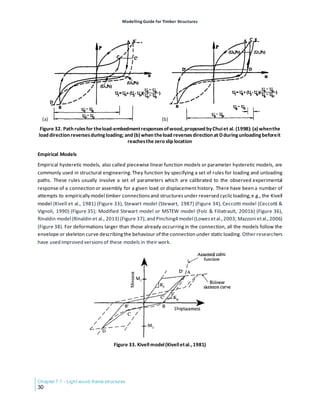

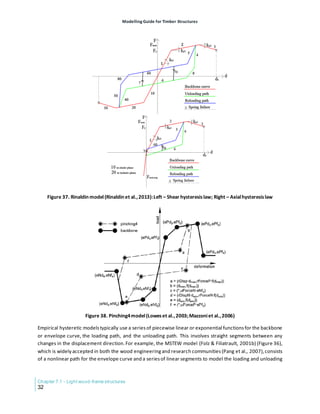
![Modelling Guide for Timber Structures
Light wood-frame structures - Chapter 7.1
33
paths off the envelope curve.Itrequiresatotal of 10 parameters(Table 1) to capture the nonlinear hysteretic
responsesof timber structures.
Table 1. Definition of hysteretic parameters of MSTEW model
Parameter Definition
K0 Initial stiffness
F0 Force intercept of the asymptotic stiffness at ultimate strength
FI Zero-displacement load intercept
Δu Displacement at ultimate load
r1 Asymptotic stiffness ratio under monotonic load
r2 Post-capping strength stiffness ratio under monotonic load
r3 Unloading stiffness ratio
r4 Reloading pinched stiffness ratio
α Hysteretic parameter for stiffness degradation
b Hysteretic parameter for stiffness and strength degradation
F0 Initial stiffness
The modelling of the monotonic pushover response of the shear wall combines an exponential and a linear
function. These two functions (Equation 13) define the ascending and descending envelopes for the lateral
load-displacement relation of the shear wall (Figure 36).
𝑭𝑭(∆) = �
sgn(∆)(𝑭𝑭𝟎𝟎 + 𝒓𝒓𝟏𝟏𝑲𝑲𝟎𝟎|∆|)�𝟏𝟏− 𝒆𝒆−𝑲𝑲𝟎𝟎|∆| 𝑭𝑭𝟎𝟎
⁄ � 𝒊𝒊𝒊𝒊 |∆| ≤ |∆𝒖𝒖|
sgn(∆)𝑭𝑭𝒖𝒖 + 𝒓𝒓𝟐𝟐𝑲𝑲𝟎𝟎[∆− sgn(∆)∆𝒖𝒖] 𝒊𝒊𝒊𝒊 |∆| > |∆𝒖𝒖|
[13]
The envelope curve is defined by five physically identifiable static parameters: 𝐾𝐾0 , 𝐹𝐹
0 , 𝑟𝑟1 , 𝑟𝑟2 , and ∆𝑢𝑢 ; see
Table 1. Phenomenologically,Equation 13 capturesthe crushingof the framing members and sheathing, along
with the yielding of the connectors. Beyond the displacement∆𝑢𝑢, which is associated with the ultimate load
𝐹𝐹
𝑢𝑢, the load-carryingcapacity decreases.
For a shear wall under cyclic loading, as illustrated in Figure 39,the load-displacementPaths OA and CD follow
the monotonic envelope curve,Equation 13.All other paths are assumed to exhibita linear load-displacement
relationship. Unloading off the envelope curve followsapath such as ABwith a stiffnessof 𝑟𝑟3 𝐾𝐾0. Here,the wall
unloads elastically. Under continued unloading,the response movesonto Path BC, which has reduced stiffness
𝑟𝑟
4 𝐾𝐾0. The low stiffness along this path exemplifiesthe pinched hysteretic response displayed by wood-frame
shear walls under cyclic loading. This occursbecause of the previously induced crushing of the wood material
of the framing members in the sheathing-to-framing nailed connections (Path BC). Loading in the opposite
direction for the firsttime forcesthe response onto the Envelope Curve CD.Unloadingoff this curve isassumed
to be elastic along Path DE, followed by a pinched response along Path EF which passes through the zero-
displacementintercept𝐹𝐹𝐼𝐼 with slope 𝑟𝑟
4 𝐾𝐾0. Continued reloadingfollowsPath FG with degrading stiffness 𝐾𝐾𝑝𝑝, as
given by
𝑲𝑲𝒑𝒑 = 𝑲𝑲𝟎𝟎 �
∆𝟎𝟎
∆𝒎𝒎𝒎𝒎𝒎𝒎
�
𝜶𝜶
[14]](https://image.slidesharecdn.com/modellingguidefortimberstructures-240325073901-2a07d971/85/Modelling-Guide-for-Timber-Structures-FPInnovations-404-320.jpg)
![Modelling Guide for Timber Structures
Chapter 7.1 - Light wood-frame structures
34
with ∆0= 𝐹𝐹
0 𝐾𝐾0
⁄ . Note (fromEquation 14) that 𝐾𝐾𝑝𝑝 is a function of the previousloading history through the last
unloading displacement ∆𝑢𝑢𝑢𝑢 off the envelope curve (correspondingto PointA in Figure 39).Thus,
∆𝒎𝒎𝒎𝒎𝒎𝒎= 𝜷𝜷∆𝒖𝒖𝒖𝒖 [15]
Figure 39. Force-displacement response ofashear wallunder cyclicloading(Folz&Filiatrault,2001b,2002a)
If the shear wall is displaced to ∆𝑢𝑢𝑢𝑢 during another cycle, then the corresponding force will be less than 𝐹𝐹
𝑢𝑢𝑢𝑢,
the value that was previously achieved. This strength degradation is shown in Figure 39 by comparing the
respective force levels reached at points A and G. In this model, under continued cycling to the same
displacement level, the force and energy dissipated per cycle is assumed to stabilise. To obtain the 10
parameters (Table 1), fit the model to a connection or to the shear wall test data by using trial-and-error
methods or specific tools, e.g., the CASHEW (Cyclic Analysis of wood SHEar Walls) program (Folz & Filiatrault,
2000).
The empirical hysteretic models with static parameters discussed above cannot capture the damage process
in timber structures. Richard et al. (2002) proposed a strength reduction based on a cumulative factor
calculated in one direction with respect to the previously achieved strength in the opposite direction. Collins
et al. (2005) defined a similar damage calculation process. Although most of these constitutive laws use
exponential functionsfor the pre-peak backbone curve and hysteresisloops,thatof Ayoub (2007) usestrilinear
functions. This model describes the damage process in detail, dividing it into four degradation phenomena:
strength reduction,decrease in unloading stiffness, decrease in accelerated stiffness, and cap degradation.
The Pang et al. (2007) evolutionary parameter hysteretic model (EPHM, Figure 40) is only defined by
exponential functions (pre and post-peak backbone; unloading and loading hysteretic loops); damage is not
cumulative. The Humbert (2010) model (Figure 41) can be considered an improvement of the Richard et al.
(2002) and Yasumura et al. (2006) models and is capable of modelling asymmetric behaviour (Humbert et al.,
2014).](https://image.slidesharecdn.com/modellingguidefortimberstructures-240325073901-2a07d971/85/Modelling-Guide-for-Timber-Structures-FPInnovations-405-320.jpg)

![Modelling Guide for Timber Structures
Chapter 7.1 - Light wood-frame structures
36
Mathematical Models
Mathematical models are also called semi-physical or phenomenological models (Ismail et al., 2009; Ma et al.,
2004). In general, they do not involve a detailed analysis of the physical behavior of a system through its
hysteresisloops; instead, they combine some physical understandingof the hysteretic system with some form
of black-box modelling(Ismail etal., 2009).The past fewdecadeshave seen proposalsfor variousmathematical
models of hysteresis. One of the most widely accepted is a differential model originally proposed by Bouc
(1967) and subsequently generalised by Wen (1976) and other researchers.This model is known as the Bouc–
Wen model and has seen extensive use to mathematically describe the hysteretic behavior of componentsand
devices in civil and mechanical engineering. It connects the restoring force and deformation through a first-
order nonlinear differential equation with unspecified parameters. By choosing suitable parameters, it is
possible to generate a large variety of different shapes for the hysteresis loops to account for strength
degradation, stiffness degradation, and even the pinching characteristics of an inelastic structure. Foliente
(1995) modified the Bouc–Wen–Baber–Noori (BWBN) model to characterise the general features of the
hysteretic behaviour of wood joints and structural systems.
Figure 42. Schematicdiagramofan inelasticsystem (Foliente,1993; Maet al.,2004)
The basis of the modified BWBN model (Figure 42) is the mass-normalised equation of motion for a single
degree of freedomsystem consisting of a mass connected in parallel to a nonlinear hysteretic spring, a linear
spring, and a viscous damper (see Equation 16):
𝒖𝒖̈ (𝒕𝒕) + 𝟐𝟐 ∙ 𝝃𝝃𝟎𝟎 ∙ 𝝎𝝎 ∙ 𝒖𝒖̇ (𝒕𝒕) + 𝜶𝜶 ∙ 𝝎𝝎𝟐𝟐 ∙ 𝒖𝒖(𝒕𝒕) + (𝟏𝟏 − 𝜶𝜶) ∙ 𝝎𝝎𝟐𝟐 ∙ 𝒛𝒛(𝒕𝒕) = 𝒇𝒇(𝒕𝒕) [16]
where 𝑢𝑢 is relative displacement of the mass to the base; 𝜉𝜉0 is the linear viscous damping ratio, which equals
𝑐𝑐𝑐𝑐𝑐𝑐 2
⁄ , where 𝑐𝑐 is linear viscous damping coefficient,𝑚𝑚 is mass, 𝜔𝜔 is the pseudo-natural frequency of the
nonlinear system, and 𝜔𝜔2
is mass-normalised stiffness; 𝛼𝛼 is arigidity ratio that determinesthe ratio of the final
asymptote tangent stiffness to the initial stiffness; 𝑓𝑓(𝑡𝑡) = 𝐹𝐹(𝑡𝑡)/𝑚𝑚, where 𝐹𝐹(𝑡𝑡) is the force applied to the
mass; and 𝑧𝑧(𝑡𝑡) is hysteretic displacement,expressed with the differential equation shown in Equation 17:
𝒛𝒛̇(𝒕𝒕) =
𝒖𝒖̇ (𝒕𝒕)−𝒗𝒗�𝜷𝜷∙|𝒖𝒖̇ (𝒕𝒕)|∙|𝒛𝒛(𝒕𝒕)|𝒏𝒏−𝟏𝟏∙𝒛𝒛(𝒕𝒕)+𝜸𝜸∙𝒖𝒖̇ (𝒕𝒕)∙|𝒛𝒛(𝒕𝒕)|𝒏𝒏�
𝜼𝜼
𝒉𝒉(𝒛𝒛) [17]](https://image.slidesharecdn.com/modellingguidefortimberstructures-240325073901-2a07d971/85/Modelling-Guide-for-Timber-Structures-FPInnovations-407-320.jpg)
![Modelling Guide for Timber Structures
Light wood-frame structures - Chapter 7.1
37
where 𝛽𝛽 and 𝛾𝛾 act as a couple and determine whether the curve is hardening or softening; n is a parameter
which determinesthe sharpnessof the transition from the initial slope to the slope of the asymptote; 𝜂𝜂 and 𝑣𝑣
are the linearly energy-based stiffness and strength degradation parameters, respectively; and ℎ(𝑧𝑧) is the
pinchingfunction given in Equation 18:
𝒉𝒉(𝒛𝒛) = 𝟏𝟏 − 𝝃𝝃𝟏𝟏 ∙ 𝒆𝒆
�−�𝒛𝒛∙𝒔𝒔𝒔𝒔𝒔𝒔�𝒖𝒖̇ (𝒕𝒕)�−𝒒𝒒∙𝒛𝒛𝒖𝒖�
𝟐𝟐
𝝃𝝃𝟐𝟐
𝟐𝟐
� �
[18]
where 𝑠𝑠𝑠𝑠𝑠𝑠 is the signum function; 𝜉𝜉1 and 𝜉𝜉2 control the pinching stiffness and pinching range, respectively;
and 𝑞𝑞 controlsthe residual force.This model can therefore representawide variety of hardeningor softening
hysteresis loops with a considerable range of cyclic energy dissipation. It includes the system degradation
(stiffness and/or strength) as a function of the hysteretic energy dissipation and pinching.
This modified BWBN model of the hysteretic behaviour of timber connectionsand structuresisgoverned by 13
differentidentifiable parametersin Eqs.(16) to (18) (Chen etal., 2014; Xu and Dolan, 2009a,b).It calibratesthe
BWBN parameters by using the response to a particular cyclic displacement history, and then evaluates the
responses for other histories or seismic excitations. Identifying the Bouc–Wen model parameters involves
proposingasignal input(or several) and an identification algorithmthat usesthe measured outputof the model
along with this input to determine the unknown model parameters. This question has stirred a lot of research
due to itsdifficulty as a nonlinear and nondifferentiable problem.Some proposed identification methodsinvolve
a rigorous analysis of the convergence of the parameters to their true values, while others rely on numerical
simulations and experimentation. Available options (Ismail et al., 2009) include (a) Least-squares identification;
(b) Kalman filter identification; (c) Geneticalgorithmidentification;(d) Gauss-Newton iterative Identification; (e)
Bootstrap filter identification; (f) Identification using periodic signals; (f) Simplex method identification; (g)
Supportvector regression identification;and (h) Constrained nonlinear optimization identification.
To simulate the highly asymmetric hysteresis of specific timber connections, e.g., hold-downs, Aloisio et al.
(2020) developed an extended energy-dependentgeneralised Bouc–Wen model (Song& Kiureghian, 2006) by
adding two energy-based parameters.Structural analysissoftware like SAP2000 and OpenSees implementsthe
Bouc–Wen,Baber–Noori–Wen,and BWBN models, in a simplified form, to predictthe nonlinear responsesof
springelements (Mazzoni et al., 2006).They have also been incorporated into the general-purpose FEsoftware
ABAQUS through subroutines (Xu & Dolan, 2009a,2009b),and also into MATLAB(Aloisio et al., 2021).
Model Comparison
Although each has its own features, most models of the same type share similar advantages and limitations.
Table 2comparesthe three major types of hysteretic modelsfor timber structures,discussed in the preceding
pages of this section and summarised below.](https://image.slidesharecdn.com/modellingguidefortimberstructures-240325073901-2a07d971/85/Modelling-Guide-for-Timber-Structures-FPInnovations-408-320.jpg)


![Modelling Guide for Timber Structures
Chapter 7.1 - Light wood-frame structures
42
American Society of Civil Engineers(ASCE). (2016).Minimum design loads and associated criteria for buildings
and other structures.
American Society of Civil Engineers (ASCE). (2017). Seismic evaluation and retrofit of existing buildings
(ASCE/SEI, 41-17).
American Wood Council (AWC).(2018).National design specification for wood construction.
APA – The Engineered Wood Association.(2001).Wood structural panel shear wall and diaphragm - Allowable
stress design manual for engineered wood construction.
Applied Technology Council (ATC). (1981).Guidelines for the design of horizontal wood diaphragms (ATC-07).
Ayoub, A. (2007). Seismic analysis of wood building structures. Engineering Structures, 29(2), 213–223.
https://doi.org/10.1016/j.engstruct.2006.04.011
Bouc, R. (1967).Force vibration of mechanical systems with hysteresis [Conference presentation].4th Conf. on
Nonlinear Oscillation, Prague,Czechoslovakia.
Building Seismic Safety Council (BSSC). (2006). Homebuilders’ guide to earthquake resistance design and
construction – FEMA P-232. Reportprepared for the Federal Emergency ManagementAgency (FEMA)
of the United States Department of Homeland Security. National Institute of Building Sciences,
Washington, D.C.
Burgess, H. J. (1976).Derivation of the wall racking formulae in TRADA's design guide for timber frame housing
(Research ReportE/RR/36). Timber Research and DevelopmentAssociation (TRADA).
Carradine, D. M. (2019). Multi-storey light timber-framed buildings in New Zealand - Engineering design.
Building Research Association of New Zealand (BRANZ).
Ceccotti, A., & Vignoli, A.(1990).Engineered timber structures: An evaluation of their seismic behaviour. In H.
Sugiyama (ed)., Proceedings of the International Timber Engineering Conference, Tokyo, Japan (pp.
946–953).
Chen, Z., Chui, Y.-H., Doudak, G., & Nott, A. (2016). Contribution of type-X gypsum wall board to the racking
performance of light-frame wood shear walls. Journal of Structural Engineering, 142(5), 04016008.
https://doi.org/10.1061/(ASCE)ST.1943-541X.0001468
Chen, Z., Chui, Y. H., Mohammad, M., Doudak, G., & Ni, C. (2014). Load distribution in lateral load resisting
elements of timber structures [Conference presentation]. World Conference on Timber Engineering,
Québec City, Québec,Canada.
Chen, Z., Chui, Y. H., Ni, C., Doudak, G., & Mohammad, M. (2014a). Load distribution in timber structures
consisting of multiple lateral load resisting elementswith differentstiffnesses. Journal of Performance
of Constructed Facilities, 28(6),A4014011.https://doi.org/10.1061/(ASCE)CF.1943-5509.0000587
Chen,Z., Chui, Y. H., Ni, C., Doudak, G., & Mohammad, M. (2014b).Simulation of the lateral driftof multi-storey
light wood frame buildings based on a modified macro-elementmodel. In A. Salenikovich (Ed.), World
Conference on Timber Engineering (WCTE 2014).
Chen, Z., Chui, Y. H., Ni, C., & Xu, J. (2014).Seismic response of midrise wood light-frame buildings with portal
frames. Journal of Structural Engineering, 140(8),A4013003.https://doi.org/10.1061/(ASCE)ST.1943-
541X.0000882
Chen, Z., & Ni, C. (2017).Seismic response of mid-rise wood-frame buildingson podium. FPInnovations.
Chen, Z., & Ni, C. (2020). Criterion for applying two-step analysis procedure to seismic design of wood-frame
buildings on concrete podium. Journal of Structural Engineering, 146(1), 04019178.
https://doi.org/10.1061/(ASCE)ST.1943-541X.0002405](https://image.slidesharecdn.com/modellingguidefortimberstructures-240325073901-2a07d971/85/Modelling-Guide-for-Timber-Structures-FPInnovations-413-320.jpg)
![Modelling Guide for Timber Structures
Light wood-frame structures - Chapter 7.1
43
Chen, Z., & Ni, C. (2021).Seismic force-modification factorsfor mid-rise wood-frame buildings with shearwalls
using wood screws. Bulletin of Earthquake Engineering, 19, 1337–1364.
https://doi.org/10.1007/s10518-020-01031-7
Chen, Z., Ni, C., Karacabeyli, E., Yeh, B., & Line, P. (2020). Expanding wood use towards 2025: Seismic
performance of midply shear walls. FPInnovations.
Christovasilis, I., & Filiatrault, A. (2010). A two-dimensional numerical model for the seismic collapse
assessment of light-frame wood structures. In S. Senapathi, K. Casey, & M. Hoit (eds.), Structures
Congress 2010 (pp. 832–843).
Chui, Y. H., Ni, C., & Jiang, L. (1998). Finite-element model for nailed wood joints under reversed cyclic load.
Journal of Structural Engineering, 124(1), 96–103. https://doi.org/10.1061/(ASCE)0733-
9445(1998)124:1(96)
Collins, M., Kasal, B., Paevere, P., & Foliente, G. C. (2005). Three-dimensional model of light frame wood
buildings. I: Model description. Journal of Structural Engineering, 131(4), 676–683.
https://doi.org/10.1061/(ASCE)0733-9445(2005)131:4(676)
Canadian Standards Association (CSA). (2019).Engineering Design in Wood.(CSA O86:19).
Dassault Systèmes. (2016).Abaqusanalysis user’s manual.
Deierlein,G., & Kanvinde, A. (2003).Woodframe project report W-23: Seismic performance of gypsum walls -
Analytical investigation. Consortium of Universitiesfor Research in Earthquake Engineering(CUREE).
Dekker,J., Kuipers,J., & Ploos van Amstel, H. (1978).Buckling strength of plywood, resultsof tests and design
recommendations. HERON, 23(4),5–59.
Di Gangi, G., Demartino, C., Quaranta, G., Vailati, M., & Liotta, M. A. (2018). Timber shear walls: Numerical
assessment of the equivalent viscous damping. In G. R. Liu & P. Trovalusci (Ed.), Proceedings of the
International Conference on Computation Methods, vol.5, 2018 (pp. 929–938).
Dolan, J. D. (1989). The dynamic response of timber shear walls. [Doctoral dissertation, University of British
Columbia]. UBC Theses and Dissertations. https://dx.doi.org/10.14288/1.0062552
Easley, J. T., Foomani, M., & Dodds, R. H. (1982). Formulas for wood shear walls. Journal of the Structural
Division, 108(11),2460–2478.https://doi.org/10.1061/JSDEAG.0006075
European Committee for Standardization (CEN). (2004). Eurocode 5: Design of timber structures – Part 1-2:
General rules – structural fire design. (Eurocode Standard EN 1995-1-2).
European Committee for Standardization (CEN). (2018). Eurocode 5: Design of timber structures - Part 1-1:
General - Common rules and rules for buildings.(Eurocode Standard EN 1995-1-1)
Federal Emergency Management Agency (FEMA). (2006).Homebuilders' guideto earthquake-resistant design
and construction. FEMA 232.https://nehrpsearch.nist.gov/static/files/FEMA/PB2007111287.pdf
Federal Emergency Management Agency (FEMA). (2012). Seismic evaluation and retrofit of multi-unit wood-
frame buildings with weak first stories. FEMA P-807.
https://store.atcouncil.org/index.php?dispatch=products.view&product_id=241
Federal Emergency Management Agency (FEMA) (2020). Short-period building collapse performance and
recommendations forimproving seismic design: Volume2 - Study of one-to-fourstory wood light-frame
buildings.FEMA P-2139-2.https://atcouncil.org/docman/fema/293-fema-p-2139-2-wood/file
Filiatrault, A.,Isoda, H., & Folz, B. (2003).Hysteretic dampingof wood framed buildings. Engineering Structures,
25(4),461–471.https://doi.org/10.1016/S0141-0296(02)00187-6](https://image.slidesharecdn.com/modellingguidefortimberstructures-240325073901-2a07d971/85/Modelling-Guide-for-Timber-Structures-FPInnovations-414-320.jpg)
![Modelling Guide for Timber Structures
Chapter 7.1 - Light wood-frame structures
44
Fischer, D., Filiatrault, A., Folz, B., Uang, C.-M., & Seible, F. (2001). CUREE woodframe project report W-06:
Shake table tests of a two-story woodframe house. Consortium of Universities for Research in
Earthquake Engineering(CUREE).
Foliente, G. C. (1993).Stochastic dynamic response of wood structural systems [Doctoral dissertation, Virginia
Polytechnic Institute and State University]. VTechWorks. http://hdl.handle.net/10919/27532
Foliente, G. C. (1995). Hysteresis modeling of wood joints and structural systems. Journal of Structural
Engineering, 121(6),1013–1022.https://doi.org/10.1061/(ASCE)0733-9445(1995)121:6(1013)
Folz, B., & Filiatrault, A. (2000). CASHEW - Version 1.0: A computer program for cyclic analysis of wood shear
walls. University of California, San Diego.
Folz, B., & Filiatrault, A. (2001a).Cyclic analysis of wood shear walls. Journal of Structural Engineering, 127(4),
433–441.https://doi.org/10.1061/(ASCE)0733-9445(2001)127:4(433)
Folz, B., & Filiatrault, A.(2001b).SAWS - Version 1.0: A computer program forthe seismic analysisof woodframe
structures. University of California, San Diego.
Folz, B., & Filiatrault, A.(2002a).A computer programfor seismic analysisof woodframe structures. Consortium
of Universitiesfor Research in Earthquake Engineering. (CUREE)
Folz, B., & Filiatrault, A. (2002b). CASHEW: A computer program for the cyclic analysis of wood shear walls.
Consortium of Universities for Research in Earthquake Engineering(CUREE).
Foschi, R. (2000). Modeling the hysteretic response of mechanical connections for wood structures. In WCTE
2000: World Conference on Timber Engineering, Whistler Resort, British Columbia, Canada, July 31–
August3, 2000.
Franco,L.,Pozza, L., Saetta, A., Savoia, M., & Talledo, D. (2019).Strategiesfor structural modellingof CLTpanels
under cyclic loading conditions. Engineering Structures, 198(1), 109476.
https://doi.org/10.1016/j.engstruct.2019.109476
Gatto, K., & Uang, C.-M. (2002). Woodframe project report W-13: Cyclic response of woodframe shearwalls:
Loading protocol and rate of loading effects. Consortium of Universities for Research in Earthquake
Engineering(CUREE).
Girhammar, U. A., & Källsner, B. (2008). Analysis of influence of imperfections on stiffness of fully anchored
light-frame timber shear walls—elastic model. Materials and Structures, 42(3), 321.
https://doi.org/10.1617/s11527-008-9458-7
He, M. (2002). Numerical modeling of three-dimensional light wood-framed buildings [Doctoral dissertation,
University of British Columbia]. UBC Theses and Dissertations. http://hdl.handle.net/2429/13092
Henrici,D. (1984).Zur Bemessung Windaussteifender Hölzerner Wandscheibe [On the design of wind-bracing
wooden wall slabs]. Bauen mit holz, 86(12),873–877.
Humbert, J. (2010). Characterization of the behavior of timber structures with metal fasteners undergoing
seismic loadings[Doctoral dissertation, Grenoble University].
Humbert,J., Boudaud, C., Baroth,J., Hameury,S., & Daudeville,L.(2014).Jointsand wood shear walls modelling
I: Constitutive law, experimental testsand FE model under quasi-static loading. Engineering Structures,
65, 52–61.https://doi.org/10.1016/j.engstruct.2014.01.047
International Code Council (ICC). (2021).The International Building Code (IBC).
Ismail, M., Ikhouane, F., & Rodellar, J. (2009). The hysteresis Bouc–Wen model, a survey. Archives of
Computational Methods in Engineering, 16(2),161–188.https://doi.org/10.1007/s11831-009-9031-8
Källsner,B. (1984).Skivor som vindstabiliserandeelement vid träregelväggar [Panelsas wind-bracingelements
in timber-framed walls]. TräteknikRapport no. 56.TräteknikCentrum.](https://image.slidesharecdn.com/modellingguidefortimberstructures-240325073901-2a07d971/85/Modelling-Guide-for-Timber-Structures-FPInnovations-415-320.jpg)
![Modelling Guide for Timber Structures
Light wood-frame structures - Chapter 7.1
45
Källsner, B., & Girhammar, U. A. (2009a). Analysis of fully anchored light-frame timber shear walls—Elastic
model. Materials and Structures, 42(3),301–320.https://doi.org/10.1617/s11527-008-9463-x
Källsner,B., & Girhammar, U. A. (2009b).Plastic models for analysis of fully anchored light-frame timber shear
walls. Engineering Structures, 31(9),2171–2181.https://doi.org/10.1016/j.engstruct.2009.03.023
Källsner,B., Girhammar, U. A., & Wu,L.(2001).A simplified plastic model for design of partially anchored wood-
framed shear walls. In CIB-W18, Meeting Thirty-Four, Venice, Italy, August2001.
Källsner, B., & Lam, F. (1995). Diaphragms and shear walls. Holzbauwerke nach Eurocode 5 - STEP 3.
ArbeitsgemeinschaftHolz.
Kivell, B. T., Moss, P. J., & Carr, A. J. (1981). Hysteretic modelling of moment-resisting nailed timber joints.
Bulletin of the New Zealand National Society for Earthquake Engineering, 14(4), 233–245.
https://doi.org/10.5459/bnzsee.14.4.233-243
Koliou, M., van de Lindt, J. W., & Hamburger, R. O. (2018). Nonlinear modeling of wood-frame shear wall
systems for performance-based earthquake engineering: Recommendationsfor the ASCE41 standard.
Journal of Structural Engineering, 144(8), 04018095. https://doi.org/10.1061/(ASCE)ST.1943-
541X.0002083
Krawinkler, H., Parisi, F., Ibarra, L., Ayoub, A., & Medina, R. (2000). Woodframe project report W-02:
Development of a testing protocol for woodframe structures. Consortium of Universities for Research
in Earthquake Engineering(CUREE).
Larsson, G., & Wästlund, G. (1953). Plywood som konstruktionsmaterial [Plywood as a structural material].
Statens kommitté för byggnadsforskning, Bulletin 21. Petterson.
Li, M., Foschi, R. O., & Lam, F. (2012). Modeling hysteretic behavior of wood shear walls with a protocol-
independent nail connection algorithm. Journal of Structural Engineering, 138(1), 99–108.
https://doi.org/10.1061/(ASCE)ST.1943-541X.0000438
Lowes, L. N., Mitra, N., & Altoontash, A. (2003). A beam-column joint model for simulating the earthquake
response of reinforced concrete frames (PEER Report2003/10).Pacific Earthquake EngineeringCenter
(PEER), University of California, Berkeley.
Ma, F., Zhang , H., Bockstedte, A., Foliente , G. C., & Paevere,P. (2004). Parameter analysis of the differential
model of hysteresis. Journal of Applied Mechanics, 71(3), 342–349.
https://doi.org/10.1115/1.1668082
Mazzoni, S., McKenna, F., Scott, M. H., & Fenves, G. L. (2006). The open system for earthquake engineering
simulation (OpenSEES) usercommand-languagemanual.Pacific Earthquake EngineeringCenter (PEER),
University of California, Berkeley.
McCutcheon,W.J. (1985).Rackingdeformationsin wood shear walls. Journal of Structural Engineering, 111(2),
257–269.https://doi.org/10.1061/(ASCE)0733-9445(1985)111:2(257)
McMullin, K. & Merrick, D. (2002). Woodframe project report W-15: Seismic performance of gypsum walls:
Experimental test program. Consortium of Universities for Research in Earthquake Engineering
(CUREE).
Mosalam, K.M., Machado, C., Gliniorz,K.-U., Naito, C., Kunzel,E., & Mahin,S. (2003).Woodframeproject report
W-19: Seismic evaluation of an asymmetric three-story woodframe building. Consortium of
Universities for Research in Earthquake Engineering(CUREE).
Neal, B. G. (Ed.) (1978).Plastic methods of structural analysis (3rd ed.). Chapman and Hall.
Newfield,G., Ni, C., & Wang, J.(2013a).Design example: Design of stacked multi-storey wood-based shear walls
using a mechanics-based approach.FPInnovations and Canadian Wood Council.](https://image.slidesharecdn.com/modellingguidefortimberstructures-240325073901-2a07d971/85/Modelling-Guide-for-Timber-Structures-FPInnovations-416-320.jpg)

![Modelling Guide for Timber Structures
Light wood-frame structures - Chapter 7.1
47
Salenikovich, A. J. (2000). The racking performance of light-frame shear walls [Doctoral dissertation, Virginia
Polytechnic and State University]. VTechWorks. http://hdl.handle.net/10919/28963
Serrette,R.L.,Encalada, J., Juadines,M., & Nguyen, H. (1997).Static rackingbehavior of plywood,OSB,gypsum,
and FiberBond walls with metal framing. Journal of Structural Engineering, 123(8), 1079–1086.
https://doi.org/10.1061/(ASCE)0733-9445(1997)123:8(1079)
Song, J., & Der Kiureghian,A. (2006).Generalized Bouc–Wen model for highly asymmetric hysteresis. Journal
of Engineering Mechanics, 132(6), 610–618. https://doi.org/10.1061/(ASCE)0733-
9399(2006)132:6(610)
Standards New Zealand. (1993).Timber Structures Standard (NZS 3603).
Steinmetz, D. (1988). Die Aussteifung von Holzhäusern am Beispiel des Holzrahmenbaus [The bracing of
wooden housesusing the example of timber frame construction].Bauen mit holz, 90(12),842–851.
Stewart, W. (1987). The seismic design of plywood sheathed shear walls [Doctoral dissertation, University of
Canterbury].UC Research Repository.http://hdl.handle.net/10092/2458
Tuomi, R. L., & McCutcheon,W. J. (1978).Racking strength of light-frame nailed walls. Journal of the Structural
Division, 104(7),1131–1140.https://doi.org/10.1061/JSDEAG.0004955
van de Lindt, J. W., Bahmani, P., Mochizuki,G., Pryor,S. E., Gershfeld,M., Tian, J., Symans, M.D., & Rammer, D.
(2016). Experimental seismic behavior of a full-scale four-story soft-story wood-frame building with
retrofits. II: Shake table test results. Journal of Structural Engineering, 142(4), E4014004.
https://doi.org/10.1061/(ASCE)ST.1943-541X.0001206
Varoglu, E., Karacabeyli, E., Stiemer, S., & Ni, C. (2006). Midply wood shear wall system: Concept and
performance in static and cyclic testing. Journal of Structural Engineering, 132(9), 1417–1425.
https://doi.org/10.1061/(ASCE)0733-9445(2006)132:9(1417)
Varoglu, E., Karacabeyli,E., Stiemer,S., Ni, C., Buitelaar, M., & Lungu,D.(2007).Midply wood shear wall system:
Performance in dynamic testing. Journal of Structural Engineering, 133(7), 1035–1042.
https://doi.org/10.1061/(ASCE)0733-9445(2007)133:7(1035)
von Halász, R., & Cziesielski, E. (1966). Berechnung und Konstruktion geleimter Träger mit Stegen aus
Furnierplatten [Calculation and design of glued beams with webs of veneer panels]. Berichte aus der
Bauforschung, 47.
Wagemann Herrera,M.A.(2021).Effectof diaphragmflexibility and strut axial stiffnesson the load distribution
in the lateral force resisting system [Master’s thesis, Universidad de Concepción]. Repositorio
Bibliotecas UdeC. http://repositorio.udec.cl/jspui/handle/11594/6534
Wen, Y.-K. (1976). Method for random vibration of hysteretic systems. Journal of the Engineering Mechanics
Division 102(2),249–263.https://doi.org/10.1061/JMCEA3.0002106
Xu, J., & Dolan, J. D. (2009a).Developmentof a wood-frame shear wall model in ABAQUS. Journal of Structural
Engineering, 135(8),977–984.https://doi.org/10.1061/(ASCE)ST.1943-541X.0000031
Xu, J., & Dolan, J. D. (2009b). Development of nailed wood joint element in ABAQUS. Journal of Structural
Engineering, 135(8),968–976.https://doi.org/10.1061/(ASCE)ST.1943-541X.0000030
Yasumura, M., Kamada, T., Imura, Y., Uesugi, M., & Daudeville,L.(2006).Pseudodynamic tests and earthquake
response analysis of timber structures II: Two-level conventional wooden structures with plywood
sheathed shear walls. Journal of Wood Science, 52(1), 69–74. https://doi.org/10.1007/s10086-005-
0729-4
Zhu, E., Chen, Z., Chen, Y., & Yan, X. (2010).Testing and FE modelling of lateral resistance of shearwalls in light
wood frame structures.Journal of Harbin Institute of Technology, 42(10),1548–1554.](https://image.slidesharecdn.com/modellingguidefortimberstructures-240325073901-2a07d971/85/Modelling-Guide-for-Timber-Structures-FPInnovations-418-320.jpg)


![Modelling Guide for Timber Structures
Mass timber structures - Chapter 7.2
7
better wind-induced response on the part of the MT shear wall system (Chen & Chui, 2017; Chen etal., 2015).
Note that without specific solutionsto efficiently transfer gravity loadsbetween wall panelsin adjacentstoreys,
MT floor panelswould reduce the lateral deformation of the storeys due to compression perpendicular-to-grain.
(a) (b) (c)
(d) (e)
Figure 8. Deflection componentsofplatform-typeCLTwalls(Gavricet al.,2015): (a)rocking; (b)sliding; (c)shear;
(d)bending; and (e)slip
For coupled-panel CLT shear walls, there are three possible types of kinematic behaviour: (a) coupled-wall
behaviour,when each wall panel (segment) rocksabout its lower corner asan independent,individual panel;
(b) single-coupled wall behaviour, when the wall panels behave as partly fixed panels with semirigid
connections between them; and (c) single wall behaviour, when the wall panels behave as a single wall with
rigid connections between them. In the first case, the vertical joint between wall panels is less stiff than the
anchoring connections, thus allowing the necessary slip between individual wall panels. When loaded with
lateral forces, connected panels behave like individual panels, rocking about each individual lower corner
(Figure 9[a]).The second possibility is an intermediate or combined behaviour: asvertical connectionsbetween
coupled-wall panelsare semirigid,small deformations(slip) of the vertical connection are possible (Figure 9[b]).
Conversely, if the vertical connection between coupled-wall panels is very stiff, the coupled walls behave
virtually the same as a single, monolithic wall panel (Figure 9[c]).
a) b) c)
Figure 9. Typesofbehaviour for adjacentwallpanels(Gavricet al.,2015): (a)coupled-panelbehaviour;
(b)combined single–coupledpanelbehaviour;and (c)single-panelbehaviour](https://image.slidesharecdn.com/modellingguidefortimberstructures-240325073901-2a07d971/85/Modelling-Guide-for-Timber-Structures-FPInnovations-427-320.jpg)

![Modelling Guide for Timber Structures
Mass timber structures - Chapter 7.2
9
block’ (Tomasi, 2014; Wallner-Novak et al., 2013),or a triangular compression zone (Schickhofer etal., 2010).
In rectangular-pattern uplift-force models, hold-downs and shear connectors within the ‘tensile zone’
(Figure 12[a]) or outside the compression zone (Figure 12[b]) can resist uplift forces equal to the tensile
strength of the hold-down. Triangular-pattern uplift-deformation models consider a triangular distribution of
the connector displacement, based on the displacement when the hold-down reaches its strength. Analyses
can either consider (Reynolds et al., 2017; Tamagnone et al., 2018) or ignore (Gavric et al., 2015; Gavric &
Popovski, 2014; Masroor etal., 2020; Pei et al., 2013) the compression zone.
(a) (b) (c)
(d) (e)
Figure 11. Tension-compressioncouple models:(a)Casagrande etal. (2016);(b)Tomasi(2014);(c)Wallner-
Novaket al. (2013);(d)GSchickhofer et al. (2010),modelI; and (e)GSchickhofer et al.,modelII(2010)
(a) (b)
Figure 12. Rectangular-pattern uplift-force models(a)with and (b)withouttensilezone (Reynoldsetal.,2017)](https://image.slidesharecdn.com/modellingguidefortimberstructures-240325073901-2a07d971/85/Modelling-Guide-for-Timber-Structures-FPInnovations-429-320.jpg)
![Modelling Guide for Timber Structures
Chapter 7.2 - Mass timber structures
10
(a) (b) (c)
Figure 13. Triangular-pattern uplift-deformationmodels: (a) Peiet al. (2013);(b)Reynoldsetal. (2017);and (c)
Gavric and Popovski(2014)
Typically, the load-carrying capacity of single-panel walls is that arising either from the pure rotation or from
the pure translation of the wall, whichever is less. The tension-compression couple models consider only the
hold-downs as resisting rotation (uplift) and design shear connectors as exclusively resisting sliding. The
rectangular-pattern uplift-force models and triangular-pattern uplift-deformation models, in addition to an
internal lever arm, also consider the vertical capacity of the shear connectors.Few models consider the shear-
uplift interaction of the forces specifically in the shear connectors (Gavric & Popovski, 2014), friction as an
addition to the shear capacity (Gavric et al., 2015; Reynolds et al., 2017; Wallner-Novak et al., 2013), or a
nonrigid base (Ringhofer,2010; Gerhard Schickhofer & Ringhofer,2012),e.g.,adeformable CLT flooringunder
the wall. For coupled- (Figure 14) or multipanel (Figure 15) CLT shear walls, the load-carrying capacity must
also account for the shear resistance of the vertical joints. Models developed by Casagrande et al. (2018),
Flatscher and Schickhofer (2016), Gavric et al. (2015), Masroor et al. (2020), and Nolet et al. (2019) can help
evaluate load-carrying capacity. Note that different models define single-panel behaviour slightly differently.
For example, Gavric et al. (2015) defined single-panel behaviour as what occurswhen there is no or almost no
slip in the vertical joints connectingtwo panels (Figure 9[c]), while Masroor et al. (2020) define it as only one
panel touchingthe foundation at the corner (Figure 15[b]).](https://image.slidesharecdn.com/modellingguidefortimberstructures-240325073901-2a07d971/85/Modelling-Guide-for-Timber-Structures-FPInnovations-430-320.jpg)


![Modelling Guide for Timber Structures
Chapter 7.2 - Mass timber structures
14
The models shown in Figure 17 are called macro, super element,or phenomenological models. Their aim is to
faithfully reproduce the global response of the shear walls (Chen & Popovski,2021c).Consequently,usersmust
calibrate the spring of the model to test results for a shear wall or to simulation results for a detailed wall
model. Different analyses require different input properties: an equivalent stiffness for linear analyses,
parametersdescribingabackbone curve for static pushover analyses, and those describinghysteresisloopsfor
nonlinear dynamic analyses. Chapter 7.1 discusses backbone curve models or hysteretic models that can be
used in the springs. A macro model with a transitional spring (Figure 17[a]) issuitable for shear walls with a low
aspect ratio or limited storeys without a prominent wall rotational effect, while one with a rotational spring
(Figure 17[b]) can consider the wall rotational effect.The advantages of such macro models are simplicity and
efficiency. The main drawback is that the representativeness of the model is limited to the specific wall
configuration used to calibrate the model.
The model shown in Figure 18 is called a micro or component-based model. Since it incorporates all
components, such a model can reproduce the global response of the shear walls based on individual
component response. These models must calibrate the constitutive law for each component based on the
resultsfrom experimental testsor on proper analytical assessments. As illustrated in Figure 18,it simulates CLT
panelsusing multi-layer or homogenousequivalentshell elements; shear connectors,hold-downs,and vertical
joints using spring elements; and the connections between the wall and the upper floor using rigid or elastic
springs. The modelling input relies on many factors, such as modelling objectives and types of analysis.
Generally, CLT panels are assigned orthotropic elastic properties (Popovski et al., 2019) because they are
designed to be capacity protected, while the connections require input on stiffness and strength.
FPInnovations’ CLT Handbook providesCLT material properties(Karacabeyli & Gagnon, 2019), which are also
available in some design software programs, e.g., Dlubal (Dlubal Software, 2021).The stiffness and strength of
a connection can be obtained by either calibrating the test resultsor using the equations provided by material
standards, e.g., CSA O86 (CSA, 2019b) and Eurocode 5 (CEN, 2018). Nonlinear time-history analysis of timber
connections requires a hysteretic model (see Chapter 7.1) capable of predicting the stiffness and strength
degradation, as well as the pinching effect.These types of models generally require an accurate calibration of
the elements that reproduce the structural behaviour of the connections. After calibration, it is possible to
simulate the structural behaviour of any structure assembled with the calibrated connections, regardless of
the geometrical configuration of the wall and the arrangement of the connections.The main drawback is the
need for numerous input parametersthat may not be available.
Other existing models are more or less similar to the component-based model, albeit with various
simplifications. For example, one can model panels as an isotropic material, with an equivalent modulus of
elasticity (Polastri et al., 2016; Pozza & Scotta, 2015) derived from the weighted mean values of the moduli
both parallel to and perpendicular to the grain, correspondingto the glued crosswise-alternated timber of the
panel; the panels are modelled using one or two springs or truss elements within a hinged frame (Mestar et
al., 2020; Pozza et al., 2015), as shown in Figure 19. The literature has proposed three main ways to simplify
the connections. As shown in Figure 19, a set of springs can simulate multiple shear connectors or vertical
joints. Figure 20 shows how all connections can be simulated using vertical and horizontal truss elements
(Follesa et al., 2013), while in Figure 21, connection zones with shell elements simulate the connections in
specific zones (Christovasilis et al., 2020; Rinaldi, Casagrande, Cimini, Follesa, & Fragiacomo, 2021). The
connection zone models can assign orthotopic material properties to these zones. With the zone for bottom
connections,for example,the equivalent shear modulus considersthe sliding deformation of the connections](https://image.slidesharecdn.com/modellingguidefortimberstructures-240325073901-2a07d971/85/Modelling-Guide-for-Timber-Structures-FPInnovations-434-320.jpg)


![Modelling Guide for Timber Structures
Mass timber structures - Chapter 7.2
17
The friction between the walls and the floor panels (or the foundation) should be ignored in most cases, as
earthquakes usually have vertical components that can reduce this effect.If this is impossible, the developed
modelsshould include these friction effectsin the stiffnessof either the shear connectionsor the vertical joints.
For multistorey buildings, wall models should also consider the influence of the floor panels between two
vertical walls, e.g., using elastoplastic springs or other equivalent methods, in order to account for the
compression deformation in the floor panels.Not doing so may lead to an overestimate of the lateral deflection
of the multistorey walls, resulting in an uneconomical design.
7.2.3.2 Balloon-Type Shear Walls
7.2.3.2.1 Structural Behaviour and Mechanisms
Besides the platform-type method discussed in the previous section (Figure 5 and Figure 22[a]), another
common approach to constructing MT buildings is the balloon-type method (Figure 22[b]) (Chen & Popovski,
2020c).Here,walls are continuousover multiple storeysand floor panels are attached to the sides of the walls
at each storey. This alleviates the accumulation of compression perpendicular-to-grain on the floor panels. It
also takes advantage of MT panels,which are manufactured at up to 20 m in length.Figure 23 shows a balloon-
type CLT buildingunder construction.
(a) (b)
Figure 22. Simplified schematicsof(a)platform-type and (b)balloon-typeCLTwalls](https://image.slidesharecdn.com/modellingguidefortimberstructures-240325073901-2a07d971/85/Modelling-Guide-for-Timber-Structures-FPInnovations-437-320.jpg)


![Modelling Guide for Timber Structures
Mass timber structures - Chapter 7.2
25
(a) (b) (c) (d) (d)
Figure 31. TypicalBRBF configurationswith BRBs: (a)Diagonalbracing(one way); (b)Diagonalbracing(zig-zag);
(c) MultistoreyX-bracing; (d)Inverted V-bracing(chevron);and (e)V-bracing
(a) (b) (c) (d) (e)
Figure 32. Eccentricallybraced frameconfigurations:thelinkisdesignated byalength,e.
Concentrically Braced Frames
CBFs (Figure 30) resist lateral loads through a vertical concentric truss system where the longitudinal axes of
the membersalign concentrically atthe joints. CBFs provide high stiffness in the linear range of their response,
thus reducingdeformations for serviceability limit state design. This is why they were originally developed to
resist wind loads. Single diagonal braced frames (Figure 30[a] and [b]) and X-braced frames (Figure 30[c] to
[e]), with energy dissipative connectionsat both endsof the braces, can usually take seismic loads, while the
configurations in Figure 30(f) to (j) are usually not recommended for seismic regions because they exhibit
relatively poor cyclic inelastic response or induce undesirable demandsin beamor column elements.From the
perspective of seismic design, the diagonal bracesin V or inverted-V(chevron) frame configurations, as well as
those in K or double K configurations, impose large,concentrated loads on the beams or columns that need to
be capacity protected. For X-braces, the capacity loads imposed on the beams from the brace tensile and
compressive resistance imbalance are usually minimal and can thus be ignored.This is especially true when the
cross-sectionsof the bracesare uniform for every two storeys or more.
All members of CBFs should be triangularly connected, with the diagonal braces within 30° to 60° of the
horizontal beam. Where possible, diagonal braces should be inclined at approximately 45°. This provides an
efficient system with lower member forces than other arrangements. Narrow braced frames with steeply
inclined braces are less stiff and are more sensitive to bending-type deformations of the entire frame. Wider
braced frames on the other hand are more stable structuresbut have more shear-type response under lateral
loads.
FPInnovations has conducted aseriesof monotonic and cyclic testsof braceswith end connections,mechanics
analysis of connection and system ductility, and seismic response analysis of BMTFs with various design](https://image.slidesharecdn.com/modellingguidefortimberstructures-240325073901-2a07d971/85/Modelling-Guide-for-Timber-Structures-FPInnovations-445-320.jpg)

![Modelling Guide for Timber Structures
Mass timber structures - Chapter 7.2
27
Eccentrically Braced Frames
EBFs (Figure 32) in steel structurescombine the advantages of high elastic stiffness and ductility at large storey
drifts(Fujimoto et al., 1972; Tanabashi etal., 1974).An EBF is aframing system in which the axial forcesinduced
in the bracesare transferred eitherto acolumn or another brace through shear and bendingin asmall segment
of the beam. This type of framing system dissipates seismic energy by controlled shear or flexural yielding in
those same small segments of the beams, called ‘links’. Architecturally, EBFs also provide more freedom for
door opening than CBFs and BRBRs. Figure 32(e) shows an EBF without links on every floor. The links in
Figure 32(d) are oriented vertically; therefore,unlike in other configurations,they are not integral parts of the
beams.
EBFs are best avoided in pure timber BTFs because the wood componentscannot act as links to dissipate the
seismic energy.However,they can be considered for hybrid BTFsin which the linksor the beams with links are
steel elements. The links in Figure 32(b) and (c) connectto the columns. Bruneau etal. (2011) have shown that
beam-to-column moment connectionsare vulnerable to brittle fracture.Meanwhile, link-to-column moment
connections are subject to both high moments and shear forces, making them even more vulnerable to the
same failure mode. It is thus highly desirable to avoid these two configurations.
In a CBF, either the diagonal bracesthemselvesor their end connectionsare designed and detailed to dissipate
energy.For an EBF, however,linksmust be properly designed and detailed for adequate strength and ductility.
All other structural components (beams outside the links, braces, columns, and connections) follow capacity
design principles(capacity protected) to remain essentially elastic during seismic response.
This chapter addresses the modelling of BTFs in typical building applications. While the emphasis here is on
CBFs and BRBRs, which will be discussed below, some aspects also apply to other types of BTFs.
7.2.3.3.2 Analytical Methods
There are no specific analytical models for braced timber frames, especially when considering the bending
stiffness of columns. However,the matrix method can analyse the forcesand deflection of the braced frames
(Chen & Popovski, 2021a),e.g., in MATLAB(Chandrasekaran, 2019). Given the availability of various software,
includinggeneral-purpose finite element(FE) software and design-oriented structural analysissoftware, the FE
methods discussed below(Section 7.2.3.3.3) are recommended for the analysisof braced timber frames. If one
needs to develop analytical models for such frames, e.g., when there is a need to analyse the repetitive
modellingof numerousconfigurations,some considerationsdiscussed in Section 7.2.3.3.3,e.g.,howto account
for the stiffness of connections,can also apply to the developmentof analytical models.
7.2.3.3.3 FE Methods
Chen et al. (2019) proposed two types of FE models for braced timber frames (Figure 34),a continuouscolumn
model and a pinned connection model.The continuous column model (Figure 34[a]) assumes the columns are
continuouselementsfrom the top to the bottom. It modelsthe columnsand horizontal beams using beam and
truss elements, respectively,both with linear elastic propertiesbecause they are typically capacity protected.
For the brace assemblies, each including a diagonal brace and two end connections, the model uses springs
with equivalent mechanical properties determined using springs in series theory. The horizontal beams are
pinned to the columns. Meanwhile, the pinned connection model (Figure 34[b]) useselastic truss elementsfor
both columns and horizontal beams, while modelling the brace assemblies with equivalent springs.](https://image.slidesharecdn.com/modellingguidefortimberstructures-240325073901-2a07d971/85/Modelling-Guide-for-Timber-Structures-FPInnovations-447-320.jpg)
![Modelling Guide for Timber Structures
Chapter 7.2 - Mass timber structures
28
Intersections among all members are modelled as pins. The columns in both models connect to the ground
using pin connections.The analysis results (Chen & Popovski,2020a; Chen etal., 2019) showed that the pinned
connection model underestimated the stiffness and fundamental frequency of the braced frames due to the
structural characteristics of the model itself, and that it concentrated the failure in a single storey/tier, thus
underestimating the strength and ductility of the BTFs. Similar findings occur in the analyses of braced steel
frames by Bruneau et al. (2011),MacRae et al. (2004),MacRae (2010),and Wada et al. (2009).Consequently,
one should use models with continuous columns (Figure 34[a]) to analyse and design BTFs. These models can
estimate the potential drift concentration in framesof differentheights, which in turn can estimate the column
stiffness required to achieve the desired performance. For preliminary analyses or an initial sizing of the
components, the pinned connection model can still be an efficientsolution.
(a) (b)
Figure 34. Schematicsofthe FEmodelsfor multistoreyBTFs: (a)continuouscolumn modeland
(b)pinned connection model
The brace assemblies play a key role in the structural performance of braced timber frames. Linear analyses,
which ignore the displacement in the energy dissipators, would provide relatively conservative results, e.g.,
lower period, higher seismic loads, and higher component forces/stresses. Nonlinear analyses, which do
consider the displacement in the energy dissipators, would provide more reliable and accurate results,
including the interstorey drift and the P-Delta effects. A conventional modelling approach for nonlinear
analyses models the brace using a linear elastic truss element, with a nonlinear spring for the connection at
each end.The material propertiesand geometric parameters of the brace serve asinput for the truss element,
and the full backbone curves or hysteresis loops of the connections provide input for the nonlinear springs.
The two end connections are usually assumed to behave identically, e.g., to yield at the same time. The test
results for a brace with riveted connections (4 × 5 rivets of 65 mm length) at two ends (Popovski, 2004),
Figure 35, however, have shown that the top and bottom connections of the brace experience significantly
differentdeformation levelsdue to a number of factors, includingvariability in wood strength properties.Once
nonlinear deformations started to develop in one of the connections, its reduced stiffness increased the
deformation demand on it, leading to a failure of that particular connection,usually referred to as ‘the weak
connection’.Neither failure nor any large deformation occurred in the other brace connection,often referred
to as the ‘strong connection’,or in the brace member itself. Figure 36 shows the hysteresis loops of the weak
connection, the strong connection, and the brace member of a typical glulam brace with two riveted
connections.To more accurately model the behaviour of the three components,one should use an equivalent](https://image.slidesharecdn.com/modellingguidefortimberstructures-240325073901-2a07d971/85/Modelling-Guide-for-Timber-Structures-FPInnovations-448-320.jpg)


![Modelling Guide for Timber Structures
Mass timber structures - Chapter 7.2
31
In general, moment-resisting frames have more deformation capacity and less stiffness than other structural
systems, such as shear walls and braced frames. In some cases, therefore, the deformation requirements,
rather than the strength requirements, can govern the design, especially in multistorey frames. Since they
allow for larger movements during an earthquake, inflexible elements attached to the frame, such as the
cladding, must accommodate this additional movement to avoid damage.
The analysis and design of moment-resisting connections in timber is usually complex, and such connections
may be expensive to construct. Consequently, the design process must carefully account for the connection
strength, stiffness,and rotational ductility. Common connectionsfor momentframesare dowel-type fasteners,
e.g., dowels(Figure 37 and Figure 38); nails (Figure 39[a]); rivets(Figure 39[b] and [c]); steel tubes (Figure 40),
with or without insert or gusset plate(s); and glued-in rod connections(Figure 41). Some special connections,
like steel nail plates (Figure 42), quick-connect moment connections (Figure 43), and self-tapping screws
(Figure 44),can also help reduce the time and resourcesrequired for assembly.There are also hybrid solutions
(Figure 45 to Figure 47) where timber elementsconnectto each other through a steel part with higher stiffness
and ductility. This chapter,however,will focuson moment-resisting connectionswith dowel-type fasteners.
(a) (b)
Figure 38. Beam-to-column momentconnectionswith (a)dowelsand (b)steelside plates(Gohlich,2015)
(a) (b) (c)
Figure 39. Portalframeconnectionswith (a)nailsand plywood gusset platesand (b)rivetsand steelgusset
platesfor the knee connection; and (c)the apex connection. (CourtesyofDr. Minghao Li)](https://image.slidesharecdn.com/modellingguidefortimberstructures-240325073901-2a07d971/85/Modelling-Guide-for-Timber-Structures-FPInnovations-451-320.jpg)


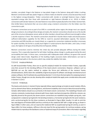

![Modelling Guide for Timber Structures
Mass timber structures - Chapter 7.2
37
7.2.4.2 Structural Non-SFRS elements
It is critical to consider structural components that resist gravity loads, such as mass timber panels, glulam
beams, glulam columns, and all their associated connections, when designing an SFRS. Review gravity
components for interstorey drift compatibility, so that the members themselves, and more specifically their
connections,can handle imparted rotations due to the overall buildinginterstorey driftwhile maintaining their
gravity load-carrying capacity under any relevant load case. This requirement is clearly laid out in the 2020
NBCC (NRC, 2022),Clause 4.1.8.3.5: ‘all structural framing elementsnot considered to be partof the SFRS must
be investigated and shown to behave elastically or to have sufficientnonlinear capacity to support their gravity
loads while undergoingearthquake induced deformations’.
In addition to maintaining their gravity load-carrying capacity, in some cases, beam-to-column connections
which should be pinned can have significant rotational capacity—something the designers may need to
consider.For instance, if a beam-to-column connection with some nominal rotational capacity is modelled as
a spring, it can engage some modest moment frame behaviour, particularly in longer frames. This moment
frame behaviour can in turn reduce the modal periodsof the global structure,and perhapseven the demands
within the primary SFRS components. This phenomenon can impact the—quite important—accuracy of the
design force within the ‘fuse’ component,and the 2020 NBCC (NRC, 2022),Clause 4.1.8.3.7,clearly laysout the
requirementto reviewit:
stiffness imparted to the structure from elements not part of the SFRS, other than those described in
sentence (6) [Walls], shall not be used to resist earthquake deflections, but shall be accounted for… a) in
calculating the period … b) in determiningthe irregularity of the structure … and c), in designingthe SFRS if
inclusion of the elementsnot part of the SFRS in the analysis has an adverse effecton the SFRS.
In practice,designersoften ignore this phenomenon of secondary stiffness added by the gravity load-resisting
frame or fail to give it the proper attention. It is certainly important to consider when heavy beam-end
connectionshave moment capacity and, in turn, can alter the lateral demand in the primary SFRS. While this
may seem onerous to consider, there is certainly precedent for such a check in standard Canadian and US
structural engineering practice. For example, there are similar provisions in the concrete material standard,
CSA A23.3-19 (CSA,2019a),under Clause 21.11,which outlinesthe requirementsfor ‘MembersNotConsidered
Part of the Seismic-Force-Resting-System Rd=1.5, 2.0, 2.5, 3.5, or 4.0)’. Clause 21.11.3 outlines requirements
for gravity load-resisting frames, and Clause 21.11.3.4 outlines requirementsfor slab-to-column connections.
Some primary requirementsare related to the aspectratiosof members,ensuringthey do notattract too much
load from the primary SFRS components,and to the ductility requirementsin detailing, to avoid brittle failures
in these gravity load-resisting components. There is very little commentary on this issue in the currentversion
of CSA O86-19 (CSA, 2019b). Clarity must be added in CSA O86, to bring it in line with the NBCC provisionson
how to explicitly consider this issue in the modelling and design of timber components and connections.
7.2.4.3 Diaphragm Stiffness Effects
For more detailed information on the modelling of various diaphragm effects, see Chapter 6.2. The structural
engineeringcommunity has long discussed the complex issue of the stiffness of mass timber diaphragms. The
assumptions underlying the modelling of the diaphragm can drastically impact the vertical SFRS components,
as they directly affectthe distribution of forces.For modelling/analysis purposes,the options are essentially as
follows:](https://image.slidesharecdn.com/modellingguidefortimberstructures-240325073901-2a07d971/85/Modelling-Guide-for-Timber-Structures-FPInnovations-457-320.jpg)

![Modelling Guide for Timber Structures
Mass timber structures - Chapter 7.2
39
Figure 50. Diaphragmsurface modelwith paneldelineationand line-typesprings
When linear line-type springs represent the stiffness of CLT spline, CLT-to-steel drag, or CLT-to-chord
connections,itis important to specifically revieweach connection.One method for determiningthe stiffnesses
of these connections is to use the slip information for screwed connections in Eurocode 5 (EN 1995-1-
1:2004+A1),asdescribed in clause 7 (CEN, 2004),which determinesthe stiffness of the connection Kser based
on the density of the timber material ρm and the diameter of the fastener d, as shown in Equation 1:
𝐾𝐾𝑠𝑠𝑠𝑠𝑠𝑠 = ρ𝑚𝑚
1.5
d/23 [1]
One should define the line springs relative to the panel’s local axes, in the same locations where the flexural
hinge or release will be defined.Figure 51 shows an example RFEM dialog box.
Figure 51. RFEMline springelementinput
Finally, note that there has been much debate on this topic, particularly for the design of CLT diaphragms.
New, simplified guidance on the issue appears in the updated 2021 Special Provisions for the Design of Wind
and Seismic (SPDWS) with Commentary (AWC, 2021). Section 4.5 of the SPDWS offers a simplified approach
with a nominal shear capacity (kN/m or kip/ft) for the diaphragm that considers dowel-type fastener
connections between the CLT panels. These fasteners require ductile failure behaviour. The SPDWS also
states that wood elements, steel drags, and chord members are to be designed for 2.0 times the forces
induced from design loads for capacity protection. These provisions however do not clarify how to model](https://image.slidesharecdn.com/modellingguidefortimberstructures-240325073901-2a07d971/85/Modelling-Guide-for-Timber-Structures-FPInnovations-459-320.jpg)

![Modelling Guide for Timber Structures
Mass timber structures - Chapter 7.2
41
7.2.6 References
Abrahamsen, R. (2018).Mjøstårnet – 18 storey timber building completed. Internationales Holzbau-Forum IHF
2018.https://www.forum-holzbau.com/pdf/32_IHF2018_Abrahamsen.pdf
American Institute of Steel Construction (AISC). (2016). Seismic provisions for structural steel buildings
(ANSI/AISC 341-16).
American Society of Civil Engineers(ASCE). (2016).Minimum design loads and associated criteria for buildings
and other structures (ASCE/SEI 7-16).
American Wood Council (AWC). (2021). Special design provisions for wind and seismic with commentary
(ANSI/AWC SDPWS-2021).
ANSI & APA. (2019).Standard for performance-rated cross-laminated timber (ANSI/APA PRG 320-2019).
Blass, H. J., & Fellmoser, P. (2004).Design of solid wood panels with cross layers.
Blass, H., & Schädle, P. (2011). Ductility aspects of reinforced and non-reinforced timber joints. Engineering
Structures, 33(11),3018–3026.
Blomgren, H.-E., Koppitz, J.-P., Valdés, A., & Ko, E. (2016).The heavy timber buckling-restrained braced frame
as a solution for commercial buildingsin regions of high seismicity [Conference presentation].World
Conference on Timber Engineering,Vienna, Austria.
Branco,J. M., & Neves,L. A.C. (2011).Robustnessof timber structuresin seismic areas. Engineering Structures,
33(11),3099–3105.
Breneman, S., McDonnell, E., & Zimmerman, R. (2016). An approach to CLT diaphragm modelling for seismic
design with application to a US high-rise project.In J. Eberhardsteiner,W.Winter, A. Fadai, & M. Pöll.
(Eds.), WCTE 2016 e-book: containing all full papers submitted to the World Conference on Timber
Engineering (WCTE 2016), August 22–25, 2016, Vienna, Austria. TU Verlag Wien.
https://resolver.obvsg.at/urn:nbn:at:at-ubtuw:3-2204
Bruneau,M., Uang, C.-M., & Sabelli, R. (2011).Ductile design of steel structures (2nd ed.). McGraw-Hill.
Buchanan, A. H. & Fairweather R. H. (1993). Seismic design of glulam structures, Bulletin of the New Zealand
National Society for Earthquake Engineering, 26(4), 415–436.
http://dx.doi.org/10.5459/bnzsee.26.4.415-436
Canadian Standards Association (CSA). (2016).Structural glued-laminated timber (CAN/CSA-O122-16).
Canadian Standards Association (CSA). (2019a).Design of concrete structures (CSA A23.3:19).
Canadian Standards Association (CSA). (2019b).Engineering design in wood (CSA O86:19).
Canadian Wood Council (CWC). (2020).WoodWorksSizer (Version 2020,v. 11).
Casagrande, D., Doudak, G., Mauro, L., & Polastri, A. (2018). Analytical approach to establishing the elastic
behavior of multipanel CLT shear walls subjected to lateral loads. Journal of Structural Engineering,
144(2),Article 04017193.https://doi.org/10.1061/(ASCE)ST.1943-541X.0001948
Casagrande, D., Rossi, S., Sartori, T., & Tomasi, R. (2016).Proposal of an analytical procedure and a simplified
numerical model for elastic response of single-storey timber shear-walls. Construction and Building
Materials, 102(2),1101–1112.https://doi.org/10.1016/j.conbuildmat.2014.12.114
Chandrasekaran, S. (2019).Advanced structural analysiswith MATLAB. CRC Press.
Chen, Z., & Chui, Y.-H. (2017). Lateral load-resisting system using mass timber panel for high-rise buildings.
Frontiers in Built Environment, 3(40). https://doi.org/10.3389/fbuil.2017.00040
Chen, Z., Chui, Y.-H., Doudak, G., & Nott, A. (](https://image.slidesharecdn.com/modellingguidefortimberstructures-240325073901-2a07d971/85/Modelling-Guide-for-Timber-Structures-FPInnovations-461-320.jpg)


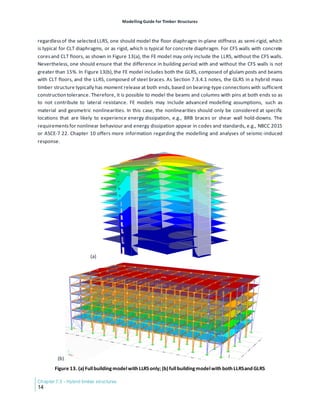
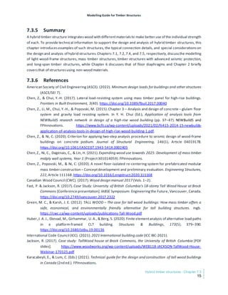


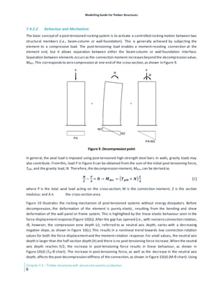


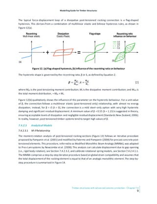


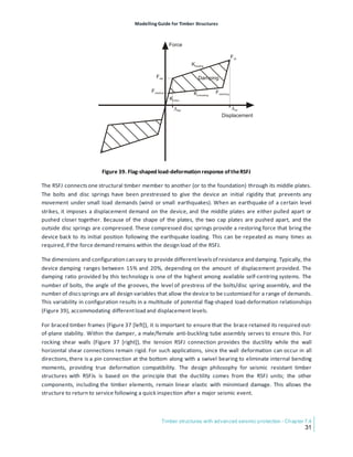

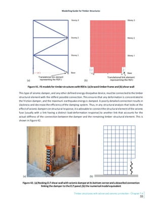


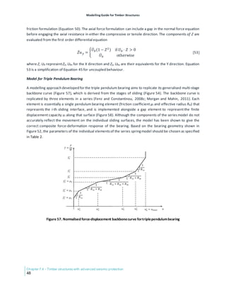


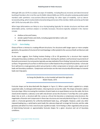


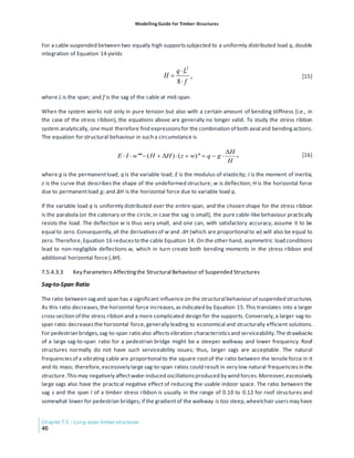


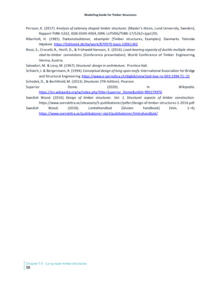


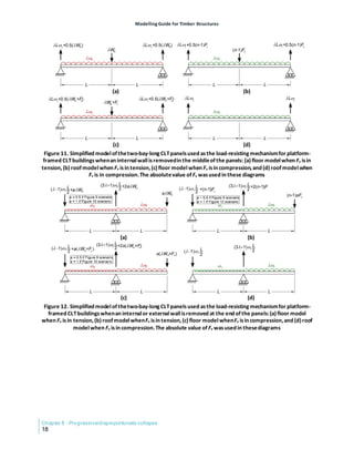


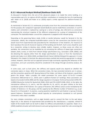


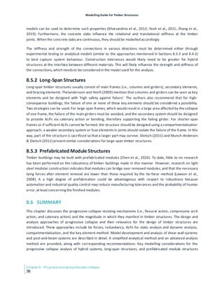


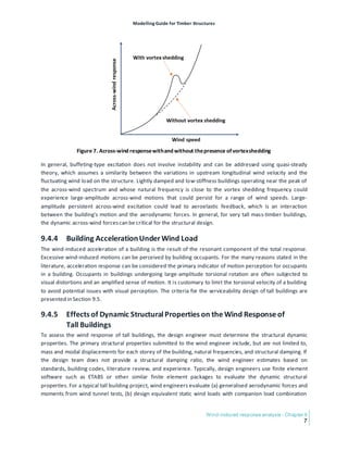
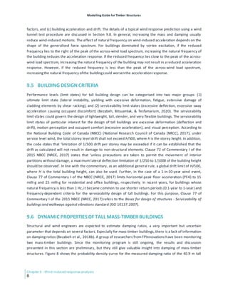


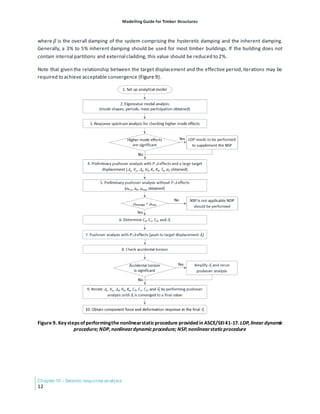


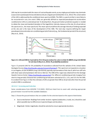


The 'Modelling Guide for Timber Structures' is a comprehensive resource developed by FPInnovations to assist engineers and researchers in the application of numerical modeling for timber structures. This first edition guide brings together the expertise of over 100 collaborators and covers essential topics including modeling principles, methods, and considerations for various timber components and connection systems. It aims to enhance understanding and application of computer modeling in timber construction, ensuring professionals can effectively design and analyze structural systems.


![Attack surfaces and attack tress[inform]](https://cdn.slidesharecdn.com/ss_thumbnails/lecture03-260108015941-a4dee53b-thumbnail.jpg?width=640&height=640&fit=bounds)


