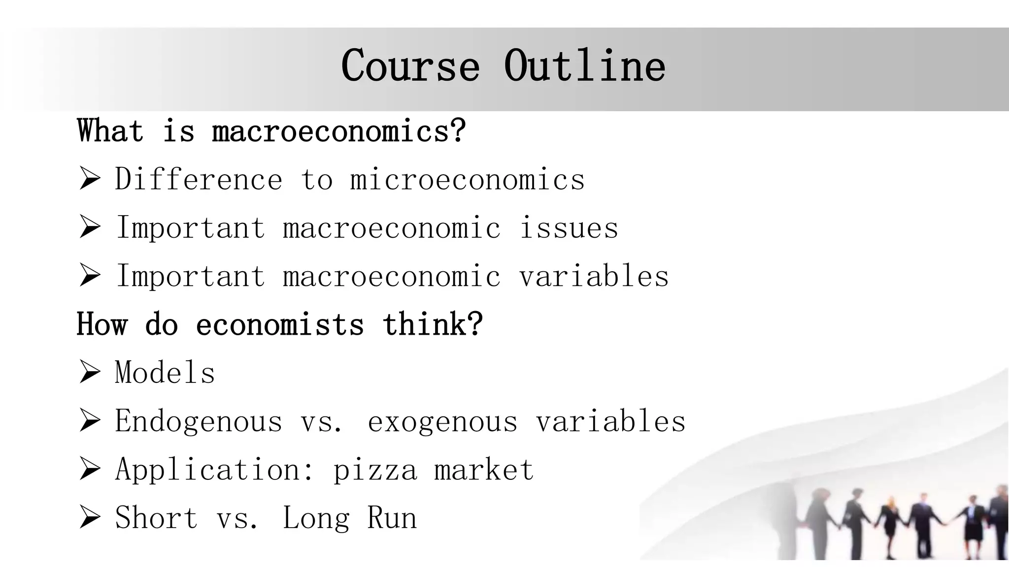
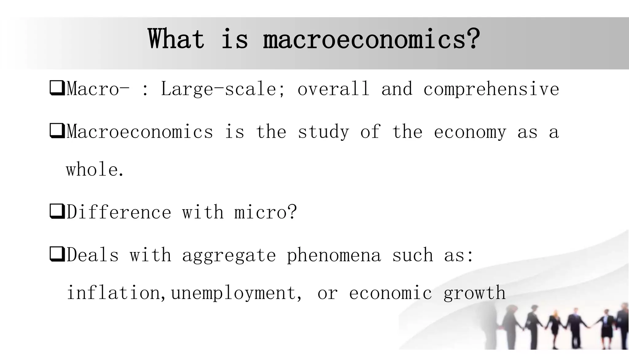
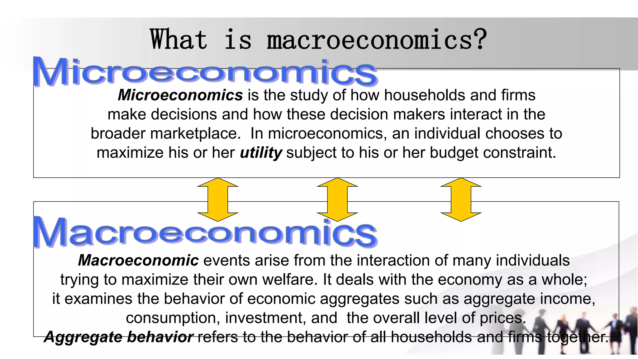
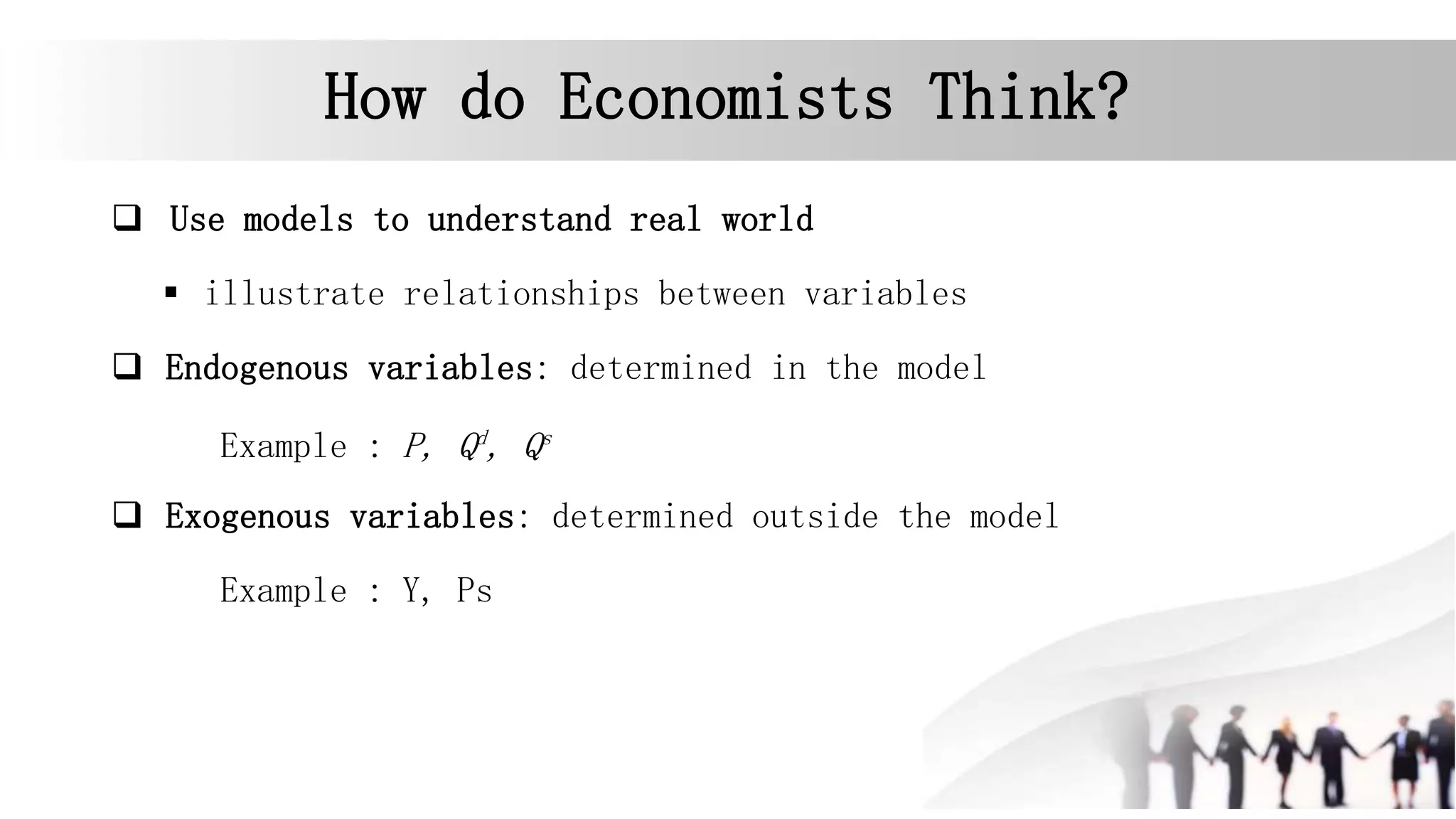
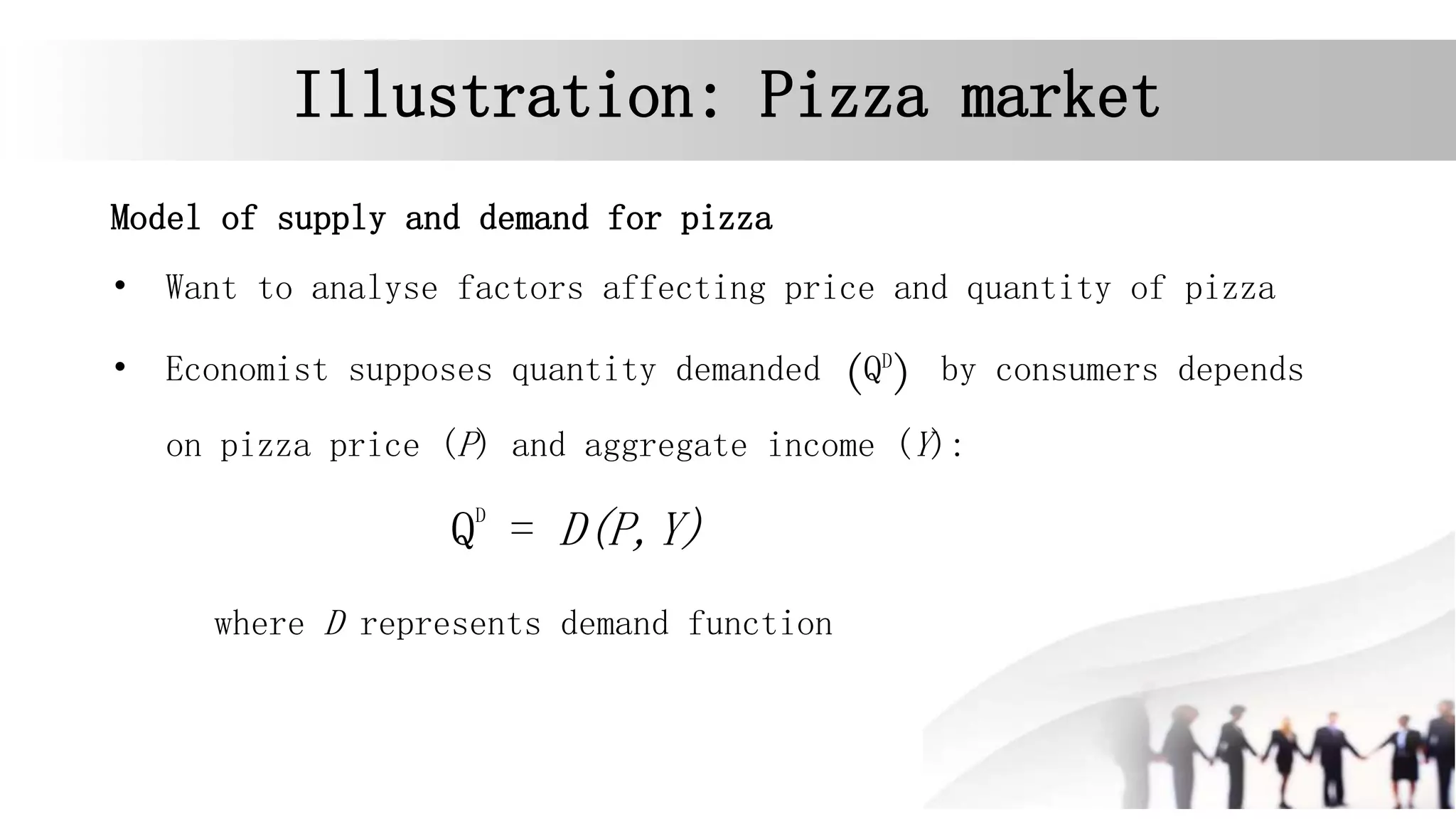
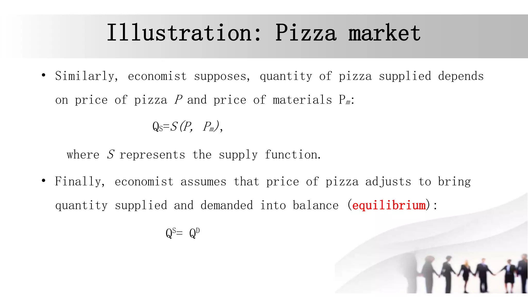
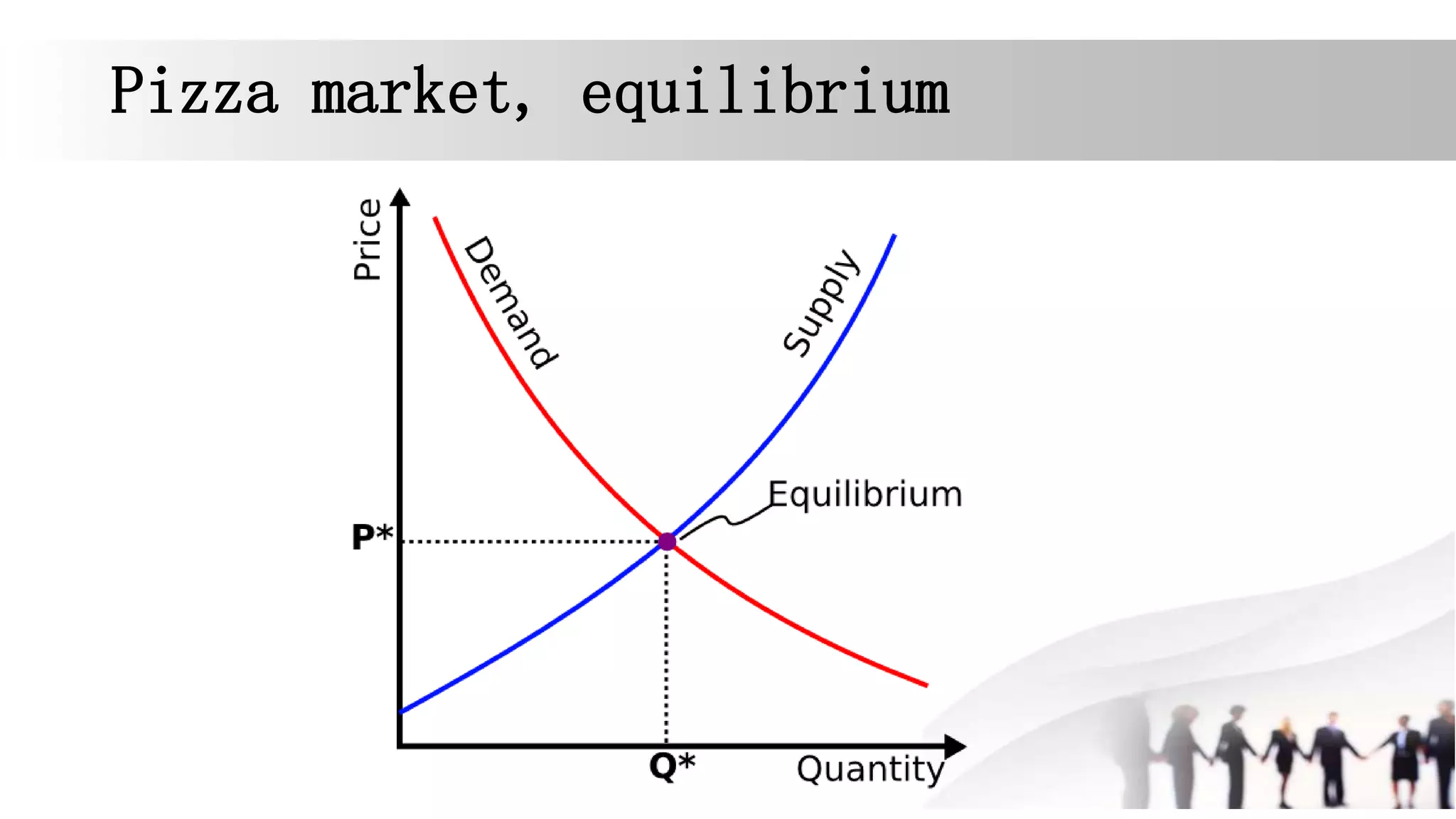
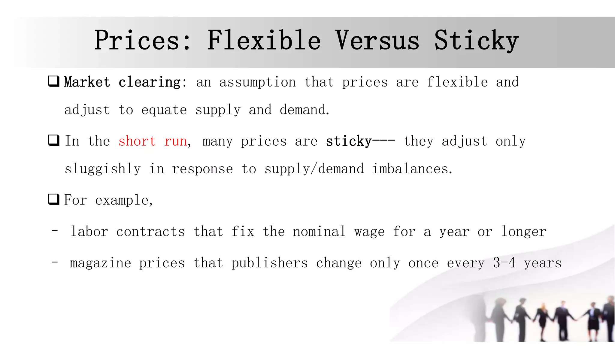
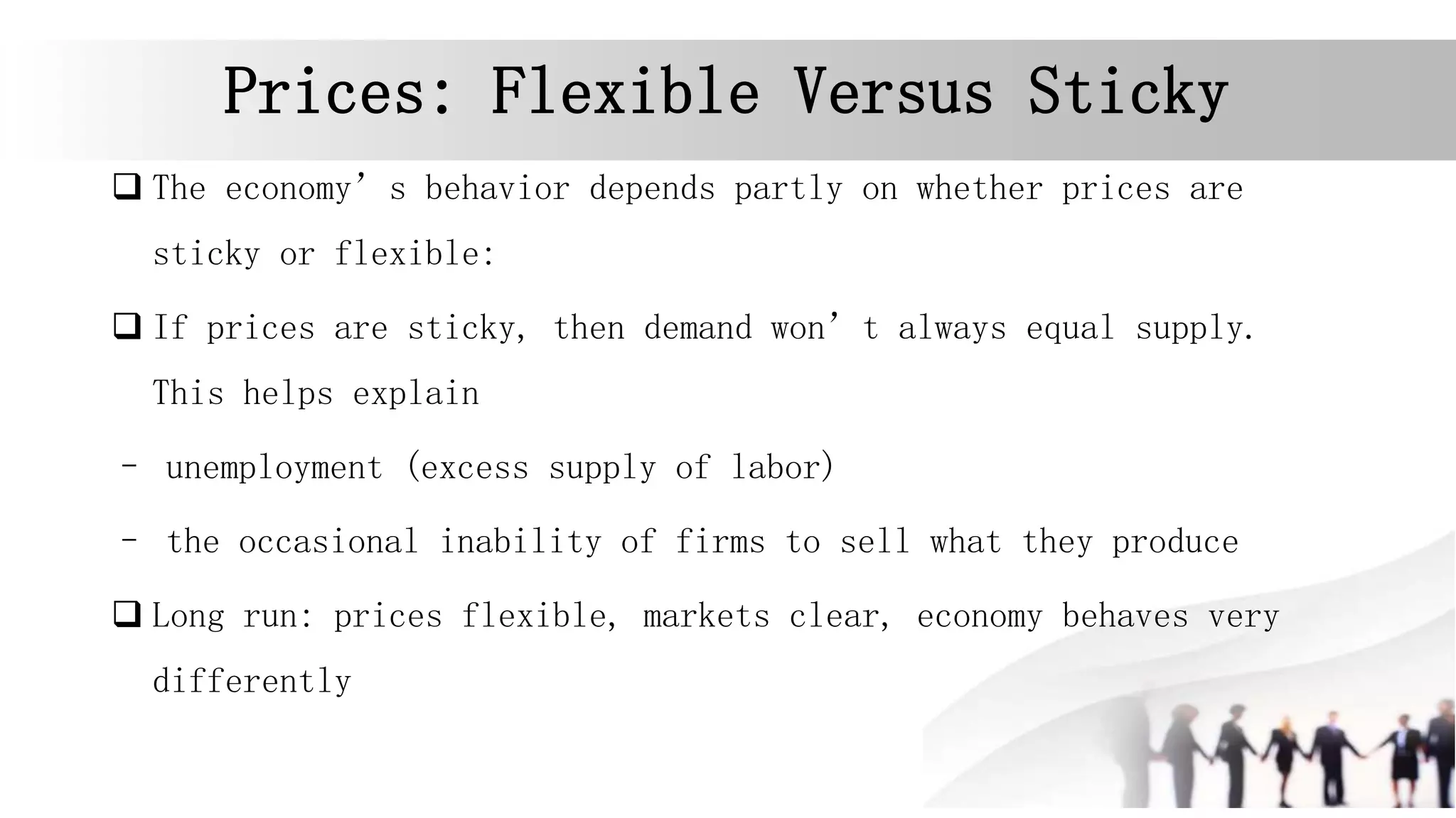
Macroeconomics examines economies at a large scale by studying aggregate variables such as output, inflation, and unemployment. It analyzes differences between the micro and macro levels. Economists use models to understand relationships between endogenous and exogenous variables in both the short-run, where prices are sticky, and long-run, where prices are flexible and technology evolves.

1. Macroeconomics
Lecture 1

2. Course Outline
What is macroeconomics?
 Difference to microeconomics
 Important macroeconomic issues
 Important macroeconomic variables
How do economists think?
 Models
 Endogenous vs. exogenous variables
 Application: pizza market
 Short vs. Long Run

3. What is macroeconomics?
Macro- : Large-scale; overall and comprehensive
Macroeconomics is the study of the economy as a
whole.
Difference with micro?
Deals with aggregate phenomena such as:
inflation,unemployment, or economic growth

4. Microeconomics is the study of how households and firms
make decisions and how these decision makers interact in the
broader marketplace. In microeconomics, an individual chooses to
maximize his or her utility subject to his or her budget constraint.
Macroeconomic events arise from the interaction of many individuals
trying to maximize their own welfare. It deals with the economy as a whole;
it examines the behavior of economic aggregates such as aggregate income,
consumption, investment, and the overall level of prices.
Aggregate behavior refers to the behavior of all households and firms together.
What is macroeconomics?

5. Three important macro variables
• Three of the major concerns of macroeconomics are:
 Gross Domestic Product
 Inflation (Why does the cost of living keep rising?)
 Unemployment (Why are millions of people unemployed, even
when an economy is booming?)

6. Gross Domestic Product (GDP)
 Symbol for real GDP: Y
 Measures total income in the economy (size of economy)
 It represents the total dollar value of all goods and service
produced over a specific time period.
 There are two variants in GDP- Nominal and Real. When nominal
GDP is adjusted for inflation, it gives real GDP.

7. GDP Malaysia
Malaysia
5% - 6%
GDP
growth
from 2016 -
2020

8. Recessions and Depressions
 Recessions: mild reductions in GDP for 2-3
quarters (is a period during which aggregate
output declines)
Aggregate output is the total quantity of goods and
services produced in an economy in a given period.
 Depressions: strong fall in GDP associated with
unusually high unemployment and often preceded
or accompanied by a financial crisis.

9. The great depression
WALL STREET IN 1929BANK RUN IN EARLY
1929

10. GDP Malaysia & Asean Countries –
Current Recession
Note:Malaysian GDP data from the Department of Statistics
Cross country comparison data from the April 2014 edition of the IMF World Economic Outlook
Euro debt crisis

11. GDP US – Current Recession
WWII Recession2008 Recession

12. Inflation and Deflation
 Inflation is an increase in the overall price level.
 Measures % change in the price level (P):
Example: Price of good today RM1, price a year later RM
1.05.
What is inflation?
5%
 Deflation is a decrease in the overall price level.
Prolonged periods of deflation can be just as damaging for
the economy as sustained inflation.

13. Inflation in Malaysia
Note: Annual and monthly variation of consumer price index in %.
Source: Department of Statistics Malaysia (DSM).
In year
2017, the
panel sees
inflation
rising to
2.7%.

14. Inflation in US
U.S. Inflation Rate
The U.S. inflation rate is measured by comparing the price of goods in one year to the price of goods in a
previous base year.

15. Unemployment
 The unemployment rate is the percentage of the labor force that
is unemployed.
 The unemployment rate is a key indicator of the economy’s
health.
 The existence of unemployment seems to imply that the aggregate
labor market is not in equilibrium.

16. Unemployment in Malaysia
Note: Unemployment, Total (% of Total Labor Force).” World Bank
Unemployment rate
in Malaysia
between 2000 and
2010 is about 3.4%

17. How do Economists Think?
 Use models to understand real world
 illustrate relationships between variables
 Endogenous variables: determined in the model
Example : P, Qd
, Qs
 Exogenous variables: determined outside the model
Example : Y, Ps

18. Illustration: Pizza market
Model of supply and demand for pizza
• Want to analyse factors affecting price and quantity of pizza
• Economist supposes quantity demanded (QD
) by consumers depends
on pizza price (P) and aggregate income (Y):
QD
= D(P,Y)
where D represents demand function

19. Illustration: Pizza market
• Similarly, economist supposes, quantity of pizza supplied depends
on price of pizza P and price of materials Pm:
QS=S(P, Pm),
where S represents the supply function.
• Finally, economist assumes that price of pizza adjusts to bring
quantity supplied and demanded into balance (equilibrium):
QS
= QD

20. Pizza market, equilibrium

21. • Increase in aggregate income
(Y)
– increases demand for pizza
(rightward shift in demand
curve)
– in equilibrium: Q↑ and P ↑
a)Shift in Demand
b)Shift in Supply
• Rise in material prices (Pm)
– reduces supply of pizza
(leftward shift in supply
curve)
– in equilibrium: Q↓ and P ↑
Q
Quantity
of pizza
P
Price
of pizza S1
D
Q1
P1
P2
Q2
S2
Q
Quantity
of pizza
P
Price
of pizza
S
D1
Q1
P1
P2
Q2
D2

22. Prices: Flexible Versus Sticky
 Market clearing: an assumption that prices are flexible and
adjust to equate supply and demand.
 In the short run, many prices are sticky--- they adjust only
sluggishly in response to supply/demand imbalances.
 For example,
– labor contracts that fix the nominal wage for a year or longer
– magazine prices that publishers change only once every 3-4 years

23. Prices: Flexible Versus Sticky
 The economy’s behavior depends partly on whether prices are
sticky or flexible:
 If prices are sticky, then demand won’t always equal supply.
This helps explain
– unemployment (excess supply of labor)
– the occasional inability of firms to sell what they produce
 Long run: prices flexible, markets clear, economy behaves very
differently

24. Short Run vs. Long Run
Short Run
 The time horizon over which the wages and prices of other inputs
to production are "sticky," or inflexible.
 Example : input prices (i.e. raw materials) because it is
constrained by long-term contracts and social factors.
 Public infrastructure (roads, bridges) given in the short run.

25. Short Run vs. Long Run
Long Run
 The period of time over which input prices have time to adjust.
 Example : Output prices (finish products sell to consumers) is
more flexible.
 Technology and fixed production factors will evolve as well
responding to market incentives.

26. Summary
 What’s macroeconomics all about?
 Observe historical data on output (Y), inflation
(π), and unemployment (u).
 What is a model? What are endogenous and
exogenous variables?
 Long-run vs. short-run (key issue: price
flexibility and technology dynamics)