mixer

1. F
undamental to the chemical pro-
cess industries (CPI) — whether
specialty or bulk chemicals,
pharmaceuticals, food products,
minerals processing, environ-
mental protection or other products or
activities — is the need for mixing.The
wide variety and complexity of mix-
ing tasks encountered in industrial
applications require careful design
and scale up to ensure that effective
mixing is achieved efficiently. Designs
based on a small range of traditional
agitators are no longer economically
acceptable. Modern impellers and the
use of physical or computer modeling
can greatly enhance performance and
reduce costs.
Mixing tasks fall into six main cat-
egories: 1. blending of miscible liquids;
2. blending of mixtures with “difficult”
rheologies (such as non-Newtonian
properties); 3. suspension of solids;
4. liquid-liquid dispersions; 5. heat
transfer; and 6. gas-liquid dispersion.
Different mixing behaviors and rules
govern each basic mixing task. To op-
timize a design, or to scale-up reliably,
these behaviors and rules need to be
understood and defined. Complex
tasks that involve two or more of the
above categories require special at-
tention. The controlling task must be
identified to determine the design and
scale-up rules to be applied.
This article addresses the first five
mixing tasks that are listed above.
Gas-liquid dispersion is a complex
subject in itself and has had
many significant advances in re-
cent years. Rather than give a very ab-
breviated summary here, we refer the
reader to Reference [2] for this topic.
In addition to agitator design and
power requirements, which are fun-
damental to mixing systems, many
other considerations also play a part
in maximizing performance. These
considerations include mechanical
aspects, seal selection, materials of
construction and surface finishes to
prevent fouling or aid cleaning. Figure
2 outlines the process and factors in-
volved in designing a suitable system.
BLENDING OF
MISCIBLE LIQUIDS
During processing, inhomogeneities
of concentration or temperature often
arise. This typically happens dur-
ing process steps such as addition of
chemicals, mass transfer, heat trans-
fer and chemical reaction. Inhomoge-
neities lead to non-uniform processing
and can negatively impact product
quality. The objective of blending is to
maintain the required degree of homo-
geneity.
Degree of homogeneity
The homogeneity at a given time, M(t),
is given by the change in concentra-
tion of a component from c0 to c(t) with
time:
M t
c c t
c c
( )
( )
=
−
− ∞
0
0 (1)
where c is the concentration after an
infinite period of time. The same rela-
tion also holds for temperature homo-
geneity. A standard target homogene-
ity is 95%. The blend time needed to
achieve a higher homogeneity can be
calculated from the equation for stan-
dard blending time since inhomogene-
ities generally decline exponentially:
t t xm x m, , ln / ln .= ⋅ −( ) ( )95 1 0 05
(2)
where x is the desired degree of ho-
mogeneity. When comparing the per-
formance of blending equipment, it
is particularly important to compare
both the blending time and the degree
of homogeneity achieved.
Turbulent blending
The dimensionless blend time charac-
teristic (Ntm) is constant for geometri-
cally similar, agitated, baffled vessels
that operate in the turbulent-flow re-
gime. Appropriate baffling is always
required in the turbulent regime,
not only to achieve efficient blend-
ing, but for all mixing tasks. Without
proper baffling, fluids will tend to
rotate in the vessel and blend times
will increase. The value of Ntm de-
pends mainly on the type of impeller
Feature ReportCover Story
46 CHEMICAL ENGINEERING WWW.CHE.COM APRIL 2006
FIGURE 1. This 1900 kW agitator-drive
unit is for a continuously operated bulk-
chemicals reactor
Ekato
Mixing Systems:
Design and Scale Up
Manyoptionsareavailabletomeet
themixingchallengesconfrontedbytheCPI.
Boththeoreticalandempiricalmethodscanhelp
theengineertofittherightsystemtothetask
Werner Himmelsbach, David Houlton,
Wolfgang Keller, Mark Lovallo
EKATO Mixing Technology

2. and the diameter ratio. Mersmann [1]
evaluated the measurement results
of various authors and determined a
simple correlation that characterized
the performance of many mixers, with
H/T = 1 and a single-stage impeller,
in terms of the impeller power number
and ratio of impeller to vessel diam-
eter. In dimensionless form his equa-
tion becomes:
N t D
T
Pom = ⋅ 


 ⋅
−
−
6 7
5 3
1 3
.
/
/
(3)
Our own measurements show that
the above equation forms a good basis
for design calculations for impellers
with large diameter ratios (D/T >
0.5), whereas the following equation
is more accurate for predicting blend
times for axial-pumping impellers
with diameter ratios in the range of
0.1 to 0.5. Accuracy is about ±10% [2]:
(4)N t D
T
Pom = ⋅ 


 ⋅
−
−
5 5
5 3
1 3
.
/
/
Circulation rate
When comparing the mixing perfor-
mance of different agitators, many
users and suppliers discuss the con-
cept of “circulation rate,” which ex-
presses the number of times that it is
necessary to circulate the vessel vol-
ume to achieve a given homogeneity.
The blend time is calculated from
the assumption that vessel contents
will be homogeneous after they have
been recirculated z times by the mixer,
where z is usually taken to be 4 or 5:
t z V
q
m = . (5)
where V is the total liquid volume
in the vessel, and q is the impeller
discharge or pumping rate, which
can be measured or estimated by cal-
culation. This theoretical method is
not as reliable as the dimensionless
mixing time method, embodied by
Equations (3) and (4), which is based
on direct measurements and scale-
up rules. The discrepancy arises be-
cause mixing is not just a function of
the main impeller discharge flow, but
also of the flow patterns generated.
Mixing for chemical reactions
For a chemical reaction to proceed, it
is necessary to intimately mix the re-
actants down to the molecular scale.
According to turbulence theory [3],
however, there is a theoretical mini-
mum size of vortex, called a micro-vor-
tex, that is generated in a turbulent
liquid. The size of the micro-vortices
is a function of the viscosity of the
liquid and the average specific power
input. Turbulence cannot help to mix
the reactants on a scale smaller than
the micro-vortex. Mixing down to the
molecular scale therefore relies on
molecular diffusion of the chemicals
within the micro-vortices.
The time for micro-mixing to occur
is, in most cases, not significant com-
pared to the macro-blend time. For
example, an aqueous solution might
typically have micro-vortices of 36 µm
and a diffusion rate of approximately
2 x 10-9 m2/s, so the micro-mixing time
would be about 0.08 s.
Engineers should, however, always
consider whether micro-mixing might
be an issue. In some cases it can be
decisive, such as when competing con-
secutive reactions occur extremely
quickly.
VISCOUS AND
NON-NEWTONIAN FLUIDS
For high-viscosity liquids, the mixing
regime changes from one in which
turbulence dominates to one in which
viscous drag forces dominate, and
agitation throughout the bulk is by no
means uniform. This non-uniformity
can be made significantly worse if the
CHEMICAL ENGINEERING WWW.CHE.COM APRIL 2006 47
����������������������
�������������������
�����������������������������
��������������������������
���������������
�����������������������
�������������
����������������������
������������������������
���������������
��������
������������������
���������
�������
�������������
��������
��������
�����������
�����
���������
����������
����������
����
�����������
��������������
�����������
����������������
��������������
��������������
�������������
�����������
���
���������������
�����������
���������
����
����
FIGURE 2. Many factors are involved
with designing an agitator system for a
given application
NOMENCLATURE
A m² heat transfer area
cw kg/kg concentration
(mass fraction)
cv m³/m³ concentration
(volume fraction)
C - impeller specific factor
used in Equ. (12)
and (17)
D m impeller diameter
dp m particle size
fc - correction factor for hin-
dered-settling velocity
g m/s² acceleration due to
gravity
H m vessel filling height
hP W/m²K heat-transfer coefficient,
process side
kMO - Metzner-Otto constant
k, kp W/mK thermal conductivity, pro-
cess side
K Pa·sm viscosity “consistency
factor”
m - viscosity “flow index”
Mt N·m shaft torque
M(t) - homogeneity (time)
njs s-1 minimum shaft speed for
suspension
N s-1 agitator speed
Ntm - dimensionless
mixing time
Nu - Nusselt number
Nu = hPT/kP
P W impeller power (transmit-
ted to fluid)
Po - impeller power number,
Po = P / ( ρ N3 D5 )
Pr - Prandtl number Pr = µc/k
Psettle W settling power
q m³/s impeller pumping rate
Q W rate of heat
Re - impeller Reynolds number,
Re = N D²ρ / µ
s - Zwietering constant, impel-
ler specific
T m vessel internal diameter
tm s mixing time
V m3 volume of fluid
vs,sh m/s settling / hindered settling
velocity
v(r) m/s local velocity at radius r
x - degree of homogeneity
z - number of recirculations to
achieve homogeneity
µ, µW Pa·s mixture viscosity, at wall
m²/s kinematic viscosity
ρl,s kg/m³ density liquid, solid
γ s-1 local shear rate
τ0, w Pa yield stress, stress at wall

3. high-viscosity mixture also exhibits
the anomalous flow properties of non-
Newtonian rheology.
The most frequently encountered
anomaly is shear thinning, where vis-
cosity decreases with increasing shear
rate according to:
Local viscosity, µ γ= ⋅ −
K m 1
or (6)
Local shear stress τ γ= ⋅K m
(7)
where γ is the local shear rate, K is the
“consistency factor” and m is the “flow
index” which describes how strongly
the apparent viscosity changes with
shear rate.
Another frequently encountered
anomaly is the so-called Herschel-
Bulkley anomaly, in which case the
mixture does not flow at all until a
certain yield stress is exceeded. The
rheological behavior of such complex
mixtures can usually be described by
the following correlation:
Local viscosity, µ
τ γ
γ
=
+ ⋅0 K m
(8)
where τ0 is the yield stress at which
flow begins.
For Newtonian fluids, τ0 is zero, m
is 1, and Equations (6) and (8) reduce
to: viscosity, µ = K, which is constant
throughout the vessel. For non-New-
tonian liquids, the effective viscos-
ity of the mixture varies throughout
the vessel. Shear rate will be highest
near the impeller, and lowest near the
vessel walls and the liquid surface.
Therefore, for shear-thinning fluids,
the apparent viscosity will be lowest
at the impeller and highest at the wall
(Figure 3). If an agitator is not cor-
rectly designed for these fluids, the
mixture in regions near the walls can
be completely stagnant. This is called
the “cavern effect”.
Designing for anomalies
The first step in assessing a design
is to calculate the power and torque
absorbed by the proposed agitator.
To do this, it is necessary to know the
local viscosity, which may vary with
shear rate. The approach of Metzner
and Otto [4] can often be used to pre-
dict local shear rate, γ, at the impeller
region. They discovered that γ in the
direct vicinity of an impeller is propor-
tional to the shaft speed.
γ = ⋅k NMO (9)
where kMO, the Metzner-Otto
constant, depends on the im-
peller design. Using the im-
peller shear rate, the local vis-
cosity can be calculated from
Equation (6) or (8). The local
viscosity can then be used to
determine the Reynolds num-
ber, Re, from which the impel-
ler’s power number, Po can be
derived. Po is a function of Re.
The absorbed power can then be
calculated using:
P P N Do= ρ 3 5
(10)
Finally, the impeller torque, Mt, can
be calculated from its speed and the
absorbed power:
Mt = P
N2 π (11)
The above describes mixing near the
impeller. To be thoroughly blended,
every part of the mixture must be in
motion. The regions that move least, or
not at all, are those most remote from
the impeller. Fluid flow at the walls can
be assessed using the “torque balance”
assumption, which is that the torque
transmitted from the impeller to the
mixture must be balanced by the shear
stress at the vessel wall, τw. This as-
sumes that there are no other internals
to complicate the model. Using this as-
sumption, τw can be calculated for a cy-
lindrical tank by:
τw
tM
C V
=
⋅
(12)
where V is the volume of the mixture
and C is a factor that is impeller-spe-
cific and determined experimentally.
For shear-thinning fluids without a
yield stress, Equations (12), (6) and
(7) can be used to calculate a local
viscosity close to the tank wall or liq-
uid surface. If the mixture has a yield
stress, τ0, it is also necessary to check
whether the predicted shear stress at
the wall is large enough to create mo-
tion (τw> τ0). If it is not, there will be
stagnant areas in the tank.
The above approach can also be
applied to empirical scale up from
pilot-scale trials to plant design. Tri-
als in a vessel with a transparent wall
and base can be used to observe the
agitator speed at which good, overall
movement is achieved. The required,
minimum shear stress at the walls
can then be calculated. This value can
be used to scale up to a geometrically
similar plant-agitator design that pro-
vides a similar flow pattern to that on
the pilot scale.
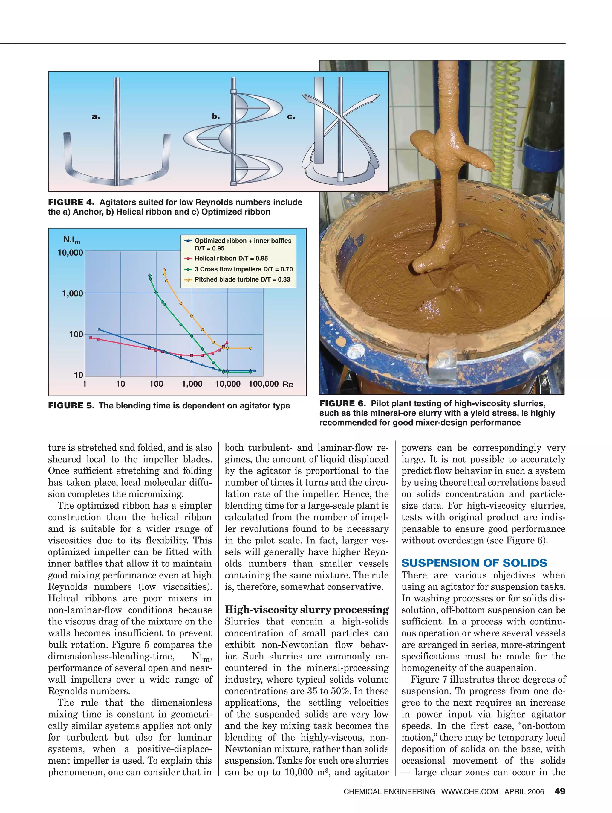
Near-wall impellers
For Reynolds numbers as low as 50,
it is possible to ensure good mix-
ing using correctly designed, large-
diameter impellers with a steep pitch.
At lower Reynolds numbers, however,
it is generally necessary to resort to
impellers that run near to the vessel
wall. Three common types are illus-
trated in Figure 4.
The anchor agitator is the simplest
form of near-wall agitator and is com-
monly in use for high-viscosity appli-
cations. The vertical arms run close
to the walls and shear the mixture as
they pass through it. Satisfactory ho-
mogeneity is not, however, efficiently
achieved since anchors create mostly
tangential displacement of the fluid.
Liquid in the center of the vessel expe-
riences little movement and the zone
around the agitator shaft is poorly
mixed.
Helical ribbon and optimized-rib-
bon impellers achieve much improved
mixing by displacing the liquid up (or
down) the wall of the vessel. The liq-
uid flows to the center of the vessel
and is then drawn in the opposite di-
rection along the axis to replace liquid
that is displaced by the agitator. Even
at extremely high viscosities of up to
1,000 Pa·s, the fluid can be circulated
throughout the entire vessel. The mix-
Cover Story
48 CHEMICAL ENGINEERING WWW.CHE.COM APRIL 2006
�
�
����
γ
•
���
γ
•
�����
�������������������
��������������������
������������γ•
������
��������������������μ�
�����������
��
����
γ
•
���
��
FIGURE 3. For shear-thinning fluids, the apparent
viscosity will be lowest at the impeller and highest
at the wall

4. ture is stretched and folded, and is also
sheared local to the impeller blades.
Once sufficient stretching and folding
has taken place, local molecular diffu-
sion completes the micromixing.
The optimized ribbon has a simpler
construction than the helical ribbon
and is suitable for a wider range of
viscosities due to its flexibility. This
optimized impeller can be fitted with
inner baffles that allow it to maintain
good mixing performance even at high
Reynolds numbers (low viscosities).
Helical ribbons are poor mixers in
non-laminar-flow conditions because
the viscous drag of the mixture on the
walls becomes insufficient to prevent
bulk rotation. Figure 5 compares the
dimensionless-blending-time, Ntm,
performance of several open and near-
wall impellers over a wide range of
Reynolds numbers.
The rule that the dimensionless
mixing time is constant in geometri-
cally similar systems applies not only
for turbulent but also for laminar
systems, when a positive-displace-
ment impeller is used. To explain this
phenomenon, one can consider that in
both turbulent- and laminar-flow re-
gimes, the amount of liquid displaced
by the agitator is proportional to the
number of times it turns and the circu-
lation rate of the impeller. Hence, the
blending time for a large-scale plant is
calculated from the number of impel-
ler revolutions found to be necessary
in the pilot scale. In fact, larger ves-
sels will generally have higher Reyn-
olds numbers than smaller vessels
containing the same mixture. The rule
is, therefore, somewhat conservative.
High-viscosity slurry processing
Slurries that contain a high-solids
concentration of small particles can
exhibit non-Newtonian flow behav-
ior. Such slurries are commonly en-
countered in the mineral-processing
industry, where typical solids volume
concentrations are 35 to 50%. In these
applications, the settling velocities
of the suspended solids are very low
and the key mixing task becomes the
blending of the highly-viscous, non-
Newtonian mixture, rather than solids
suspension.Tanks for such ore slurries
can be up to 10,000 m³, and agitator
powers can be correspondingly very
large. It is not possible to accurately
predict flow behavior in such a system
by using theoretical correlations based
on solids concentration and particle-
size data. For high-viscosity slurries,
tests with original product are indis-
pensable to ensure good performance
without overdesign (see Figure 6).
SUSPENSION OF SOLIDS
There are various objectives when
using an agitator for suspension tasks.
In washing processes or for solids dis-
solution, off-bottom suspension can be
sufficient. In a process with continu-
ous operation or where several vessels
are arranged in series, more-stringent
specifications must be made for the
homogeneity of the suspension.
Figure 7 illustrates three degrees of
suspension. To progress from one de-
gree to the next requires an increase
in power input via higher agitator
speeds. In the first case, “on-bottom
motion,” there may be temporary local
deposition of solids on the base, with
occasional movement of the solids
— large clear zones can occur in the
����
��
������
�����
���
��
� �� ��� ����� ������ �������
���������������������������������
����������
�������������������������
����������������������������������
���������������������������������
FIGURE 4. Agitators suited for low Reynolds numbers include
the a) Anchor, b) Helical ribbon and c) Optimized ribbon
CHEMICAL ENGINEERING WWW.CHE.COM APRIL 2006 49
a. b. c.
FIGURE 5. The blending time is dependent on agitator type FIGURE 6. Pilot plant testing of high-viscosity slurries,
such as this mineral-ore slurry with a yield stress, is highly
recommended for good mixer-design performance

5. upper part of the vessel. In the second
case of “off-bottom suspension,” no
particle comes to rest for longer than
one second on the bottom of the ves-
sel. This criterion, often used for large-
scale, mineral-processing applications,
defines the lowest mixing power at
which the entire surface area of the
particles is exposed to the liquid phase
for chemical reaction or mass transfer.
Zwietering [5] produced the following
well-known correlation for minimum
shaft speeds, njs, at which “off-bottom
suspension” occurs:
n s v
g
d c Djs
s l
l
p w= ⋅ ⋅
⋅ −( )




 ⋅ ⋅ ⋅ −0 1
0 45
0 2 0 13 0 85.
.
. . .ρ ρ
ρ
(13)
The third case is “visually uniform
suspension,” which is defined as hav-
ing no large clear zones. Settling of
coarse particles may still occur for sol-
ids with a wide range of particle sizes.
Occasionally, for very demanding
duties such as continuous-overflow op-
eration, or manufacture of dispersions
as end products, “uniform suspension”
is required. In this case, particle con-
centration and size distribution are
uniform throughout the vessel. This
is very difficult to achieve unless the
particle settling velocity is very low.
Design fundamentals
In addition to agitator parameters and
the vessel geometry, the properties of
both the liquid and the solid particles
influence the fluid-particle hydrody-
namics and, thus, the suspension. The
important physical properties for agi-
tator design are: the liquid density, the
density difference between solids and
liquid, the liquid viscosity, the average
particle size and the volumetric con-
centration of the solids.
A single particle’s free-settling veloc-
ity, vs, is calculated by methods given
in the relevant literature. The hinder-
ing effect on the settling process due
to the presence of several particles is
quantified by the following relation,
where the exponent m is a function
of the particle Reynolds number, and
varies between 2.33 and 4.65:
v v csh s v
m
= −( )1
(14)
where vsh is the hindered settling ve-
locity, vs is the free-settling velocity
and cv is the volume fraction of solids.
If it is assumed that all solid particles
in the liquid are distributed uniformly,
and all simultaneously begin to settle
under the effect of gravity, they re-
lease a “settling power”, which can be
quantified by the relation:
(15)P v c g Vsettle sh v= ⋅ ⋅ ⋅ ⋅∆ρ
where is the difference in density
between solid and liquid. In order to
maintain a defined degree of unifor-
mity in the suspension, the agitator
must provide a power input to the
liquid that counteracts this settling
power. The agitator power always
amounts to a multiple of the settling
power.
When one is using the above Equa-
tions (14) and (15), the choice of par-
ticle size that is used to calculate the
free-settling velocity, vs, is very impor-
tant. In powders or slurries, the indi-
vidual particles vary in size and shape.
Choosing the largest particle size can
result in a much higher agitator power
than is required. From experience, re-
liable results are obtained with a de-
sign particle size that corresponds to a
value where between 80 and 90% pass
through the mesh size.
Scale up
Scale up of suspension duties can be
very complex. Various scale up criteria
have been proposed based on the type
of suspension needed, as discussed
earlier. Specific process or product re-
quirements can impose additional cri-
teria for consideration. Some common
complications include these:
• Solids with extremely wide particle
size distributions — the fine par-
ticles affect the suspension of the
large particles
• Very high-solids concentrations —
particle interactions affect the ap-
parent rheology
• Presence of small amounts of ex-
tremely large particles — impos-
sible to suspend but must be moved
around on the base of the vessel
• The presence of significant quanti-
ties of extremely small particles
— these essentially behave as part
of the fluid
To accommodate these considerations,
solid-suspension duties are generally
Cover Story
50 CHEMICAL ENGINEERING WWW.CHE.COM APRIL 2006
FIGURE 7.
The degree of
suspension
desired for a
given applica-
tion depends
on the objec-
tive. Here,
three levels of
suspension are
shown, each
requiring more
power input
than the one
before
��
��
��
�
�
�
��������������
���������������������
��
���
��
�
���������������������
����������
��������
��������
�������
��������
��������
�
���
���
���
���
����
���
���
� � � ���
� �� �
��������������������������������������
������������������������������������������
�
�
�
�
�
�
�
��
���
���
���
�����
�����
�����
�
�
�
�
�
�
�
�� �����
FIGURE 8. To
describe the
complex nature
of suspension
tasks, suspen-
sion duties
are classified
into four broad
groups

6. classified into four broad categories on
the basis of hindered-settling velocity
(see Figure 8).
Type I tasks are simple suspend-
ing duties that are readily predicted
because the liquid flows around the
particles in simple, laminar flow. Type
II are demanding suspension tasks
where the fluid flow is more complex
but predictable from empirical corre-
lations — this category covers the ma-
jority of industrial applications. Type
III are difficult or "heavy" suspension
tasks, which probably involving large
or heavy particles. In this category,
scale-up is usually based on pilot-
scale tests. For type IV tasks, uniform
suspension is no longer attainable, as
they require very high liquid velocities
that cannot be achieved economically.
In general, for solids suspension, the
agitator power requirement is scaled
up as a function of tank diameter ac-
cording to the following equation:
(16)
P
V
DX
∝
where X can vary from 0 to -1 depend-
ing on the type of suspension duty. For
example, if particles with a high hin-
dered-settling velocity must be kept in
visually uniform suspension (Type III
in Fig. 8), a criterion close to constant
specific power input P/V must be used
(X = 0). For solids with low hindered-
settling velocities, a criterion closer to
constant tip speed (X = -1) can be used
(Type I in Fig. 8). These examples il-
lustrate how the specific power inputs
required to achieve “suspension” can
vary hugely on an industrial scale.
To achieve homogeneous suspension
of true suspensions, high-efficiency,
axial-pumping impellers are gener-
ally used because of the lower power
inputs required.
Special considerations
Some considerations for specific sus-
pension applications are as follows:
• In many solids-suspension tasks, es-
pecially in the minerals-processing
industries, abrasion can be a signifi-
cant issue. In this case, lower veloci-
ties may be required to limit abra-
sion. An increased impeller size can
compensate for the lower velocities.
• During power failures, sediments
can quickly build up in suspension
tanks. Impellers are often designed
to withstand attempted restarts,
while submerged in a densely settled
slurry. In some instances, “restart in
slurry” becomes the key design cri-
terion.
• Solids suspension and gas dispersion
commonly occur simultaneously in
the chemical- and minerals-process-
ing industries. The presence of gas
affects the performance of the impel-
ler and the ability of the fluid to sus-
pend solids. Likewise, the presence
of solids affects gas dispersion. Both
must be taken under consideration.
Additional factors that can have a
severe impact on the agitator design
include: the shape of the base of the
vessel (dished, conical or flat); the lo-
cation of the draw-off point; and the
aspect ratio (H/T) of the tank. Con-
tinuous processes are most sensitive
to such factors.
LIQUID-LIQUID
DISPERSIONS
Many industrial processes require the
dispersion of one liquid into another,
immiscible liquid. Unstable disper-
sions are created in processes such as
solvent extraction (to provide a large
surface area for mass transfer), and in
dispersion polymerizations (to create
the required size distribution of poly-
mer particles or provide a heat sink).
In the case of solvent extraction,
the dispersion must be fine enough to
allow rapid mass transfer and keep
the size of the extractor down, while at
the same time, the dispersion should
be coarse enough to enable rapid
separation of the phases afterwards.
Mixer-settler systems can generally
use finer dispersions than solvent-ex-
traction columns. The former systems
are generally better suited to slower
extractions, and the latter to fast ex-
tractions. Typical industrial applica-
tions of solvent extraction are refining
of metals from acid leach liquor and
purification of pharmaceutical prod-
ucts.
Surfactants are often used to aid
formation of the correct dispersion
size and to hinder recoalescence, in
both temporary and stable emulsions.
The interaction of the various factors
affecting dispersion processes is very
complex and nearly always necessi-
tates mixing tests. The main factors
affecting dispersion include these:
1. Physical properties of the liquids
(especially interfacial tension)
2. Effects due to mutual solubility or
reaction
3. The presence of surfactants, and
4. The turbulence and shear created
by the agitator.
Most liquid-liquid dispersions are
formed in the turbulent regime and
droplet sizes of between 5 and 500 m
can be achieved. Typically, for a spe-
cific power input of 1 W/kg, droplet
sizes between 100 and 150 m can be
expected.
Droplets break when shear stresses
induced in the droplets by turbulence
cause sufficient deformation to over-
come the stabilizing effect of surface
tension. Minimum droplet size is gov-
erned by the size of the micro-vorti-
ces, and is generally between 3 and
5 times the size of the micro-vortices.
When finer dispersions are required,
rotor-stator devices that produce a
zone of very high energy dissipation
can be used. Stabilizers can be added
to ensure that fine droplets produced
in this high-energy zone do not re-
coalesce in the bulk. For even finer
emulsions (from 5 m to 50 nanome-
ters), high-pressure homogenizers
with local energy dissipations of over
500 W/kg are used.
Scale up
Due to the complexity of the interact-
ing factors that affect droplet forma-
tion, actual performance is usually
measured in pilot trials. Because of
CHEMICAL ENGINEERING WWW.CHE.COM APRIL 2006 51
FIGURE 9. High viscosities can hin-
der heat transfer. Wall scrapers added
to an agitator, such as this optimized
ribbon, can help increase heat transfer
substantially

7. the sensitivity of surface properties
to minor levels of contaminants, pilot
trials should use actual chemicals
from the process plant rather than
laboratory-quality reagents. Scale
up to production should follow rules
that are based on the mechanism
(bulk or local turbulence) which was
used to achieve the required perfor-
mance.
HEAT TRANSFER
Stirred vessels are rarely used purely
for heat transfer because equipment
with much more-efficient heat ex-
change is available. Heat transfer is,
however, a critical unit operation that
stirred vessels must be capable of per-
forming. A typical batch process, for
example, could comprise the heating
of the bulk to reaction temperature,
blending and cooling during the reac-
tion to remove the reaction heat, fur-
ther heating to evaporate a solvent,
and finally cooling down to near ambi-
ent temperature before the product is
discharged.
Heat transfer performance is gov-
erned by:
• The flowrate and temperature of the
utilities, and heating/cooling me-
dium
• The heat-transfer coefficients on the
product side and the utility side
• The type and contact area of heat
exchange surfaces
Some of these factors may need to be
modified in order to achieve required
heat fluxes. In many reactors, the ves-
sel, itself, provides insufficient surface
area and it is necessary to install ad-
ditional heat-transfer surfaces.
Design
Heat-transfer coefficients in jackets,
coils and plate heat exchangers can be
predicted from well established corre-
lations [2]. Since the range of utility
fluids encountered is quite small and
their physical and thermodynamic
properties are generally well docu-
mented, the accuracy of predicted film
coefficients is often very good.
On the process side, however, pre-
diction of the heat transfer coefficient
is based on a general equation of the
form:
Nu
h T
k
CP
P W
=
⋅
= ⋅ ⋅ ⋅Re Pr ( )/ / .2 3 1 3 0 14µ
µ (17)
where the constant C, which depends
on the impeller type and size, can
be found in the literature or derived
by measurements. The viscosity
FIGURE 10. Modern-day impeller systems offer a great range of choice to help meet the mixing challenges facing the CPI
References
1. Mersmann, K., Chemie Ingenieur Technik,
Vol. 23, pp. 953-956, 1975.
2. EKATO (Ed), “Handbook of Mixing Tech-
nology”, EKATO Rühr- und Mischtechnik,
Schopfheim, Germany, 2000.
3. Kolmogorov, A. N., Die lokale Struktur der
Turbulenz in einer inkompressiblen zähen
Flüssigkeit bei sehr großen Reynoldsschen
Zahlen. Goering, H. (Ed) “Sammelband
zur statistischen Theorie der Turbulenz”,
Akademie-Verlag, Berlin, Germany, 1958.
4. Metzner A.B. and Otto R.E., Agitation of non-
Newtonian fluids, AIChE J, Vol. 3, No. 1, pp.
3-10, 1957.
5. Zwietering T.N., Chemical Engineering Sci-
ence, Vol. 8, pp. 244-253, 1958.
6. DeLaplace, G., others, Numerical simulation
of flow of Newtonian fluids in an agitated
vessel with a non standard helical ribbon im-
peller, “Proceedings 10th European Mixing
Conference”, Elsevier 2000.
7. Zlokarnik, M., Rührtechnik: “Theorie und
Praxis”, Springer-Verlag, Berlin, Germany,
1999.
8. “Autorenkollektiv, Mischen und Rühren,
Grundlagen und moderne Verfahren für die
Praxis,” VDI-GVC, 1998
9. Perry, R.H. and Green, D.W., “Perry’s Chemical
Engineers’ Handbook,” 7th ed., McGraw-Hill,
1997.
10. Paul E.L. and others (Eds.). “Handbook of In-
dustrial Mixing: Science and Practice,” John
Wiley Inc, New Jersey, 2004.
11. Kraume, M. and Zehner, P, Experience with
experimental standards for measurement of
various parameters in stirred tanks, TransI-
ChemE, Vol. 79, 2001.
12. Mezaki, R., others, “Engineering Data on
Mixing”, Elsevier 2000.
Cover Story
52 CHEMICAL ENGINEERING WWW.CHE.COM APRIL 2006
����������
������������
������������
�����
��������������
�������� �
�
�
�����������������������������
�����������������������������������������
�
�
�
�
�
� � �
�
�
�
��
�
��
��
��
��������������������������
����������������������������������
��
�� ��
�� ��
��
��
��
��
� �
�
�
���� ��
�� �� ��
��
��
��
��
��
��
��
��
�
����������
����������
����������
����������
�������������
����������
�������������
�������������
������������
���������

8. term represents the effect of viscos-
ity changes in the boundary layer
at the heat transfer surface. For in-
ternal components, such as coils, the
value of C differs from that for the
vessel wall. A further complication is
that physical properties of the vessel
contents are often changing during
processing — due not only to chang-
ing operating conditions, but also to
physical or chemical processes that
are occurring.
The design engineer is often faced
with the problem that the required
heat flux cannot be achieved with
existing conditions such as heat-ex-
change area or utility temperatures.
Here are some common reasons and
suggested remedies:
Effect of scale: Heat generated by a
reaction increases proportionally with
the volume of the mixture (QR ∝ V).
For geometrically similar equipment,
however, the area for heat exchange
increases proportionally to the vol-
ume raised to the power 2/3 (A ∝ V2/3).
A reaction that was simple to control
through wall cooling at the pilot scale
may therefore require additional heat-
ing/cooling surfaces in order to increase
the surface area lost on scale-up. Tube
bundles or coils mounted in the reac-
tor are often used. In cases where very
high surface areas are required, verti-
cal plate heat exchangers mounted ap-
proximately radially in the reactor can
provide as much as 25 m²/m³.
Viscosity: The material property that
commonly governs heat exchange is
viscosity, µ. In industrial applications,
the viscosity of mixtures can range
widely, such as from 0.1 to 106 mPa·s.
Because the heat transfer coefficient
is proportional to µ-1/3, the coefficients
for high-viscosity fluids are much
lower than those for low-viscosity ap-
plications. An increase in viscosity can
also mean that a liquid is no longer
in the turbulent regime, so tempera-
ture differences within the mixture
would increase. These issues are best
addressed by careful selection of the
agitator to ensure good homogeneity
across the range of operating condi-
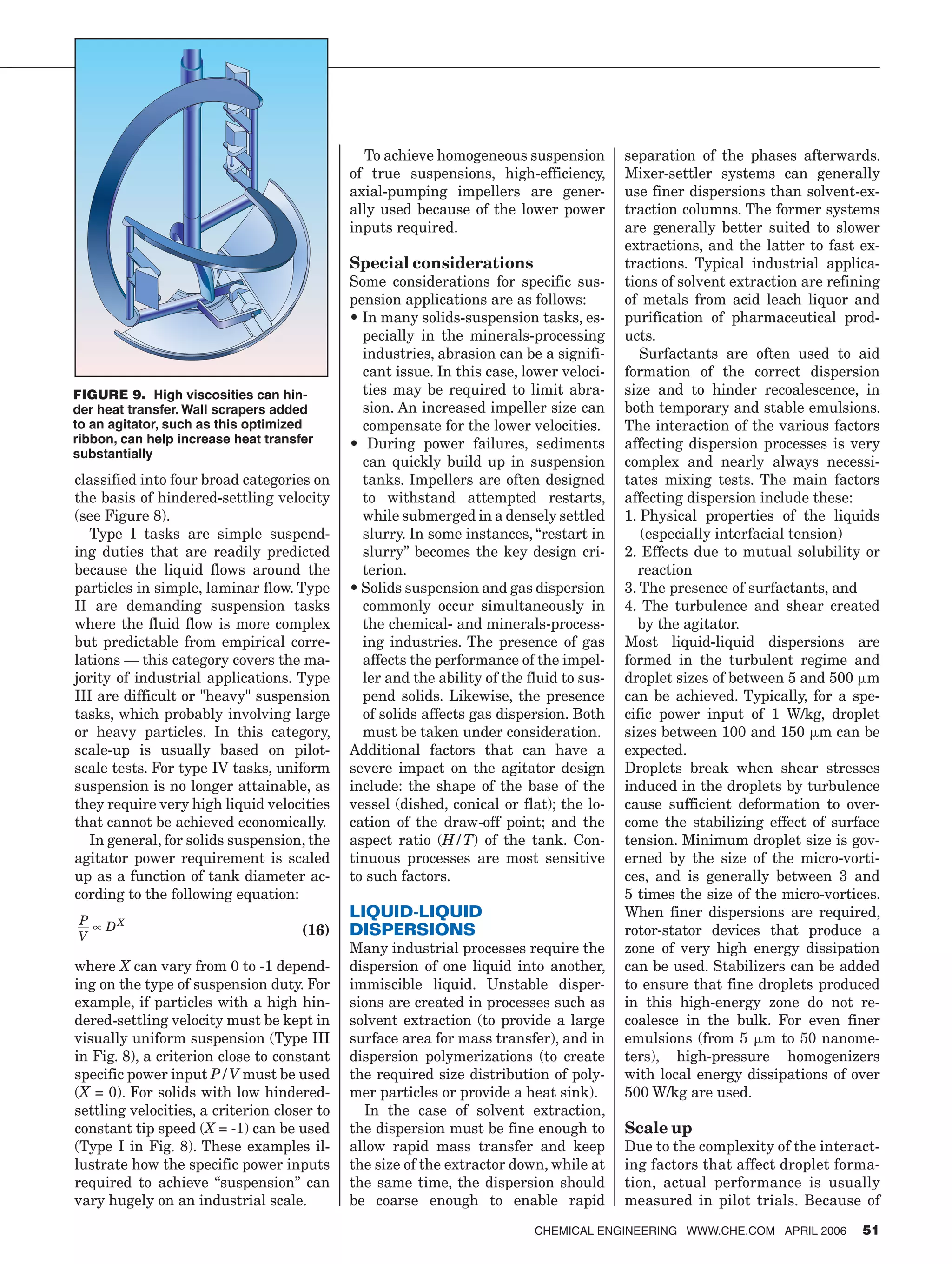
tions. Consideration should be given
to close-clearance impellers, such as
the helical ribbon and the optimized
ribbon, which increase shear and
therefore heat transfer at the wall. In
difficult cases, the use of wall scrapers
(Figure 9) can further increase heat
transfer by a factor of up to 10.
Wall fouling: Fouling is a risk in
many processes. In cooling crystal-
lization, for example, the liquid can
become supersaturated in the wall-
boundary layer. Scrapers may help,
but they are subject to wear in the
solid layer. In this case, it is better to
change the process to use cooling by
evaporation. This process may require
operation under vacuum, which brings
another consideration — flow veloci-
ties at the liquid surface must be fast
enough to avoid increased local over-
concentrations that can lead to crys-
tal nucleation. Impellers with good
axial-pumping efficiency are used to
maintain concentration and tempera-
ture homogeneity and ensure uniform
crystal growth.
Pressure vessels: Wall thicknesses
can become the limiting factor for
heat transfer, especially with stainless
steel vessels that contain a low-viscos-
ity fluid. It is not possible, for exam-
ple, to achieve an overall heat trans-
fer coefficient above 300 W/m²K if the
wall thickness is 50 mm. This overall
heat-transfer coefficient cannot be
improved by more intense agitation.
Similarly, deposits on the utility side
of the jacket or heat-transfer surfaces
can build up and cause poor thermal
conductivity. Only a few millimeters of
deposit can have a detrimental effect
on the heat transfer. Regular cleaning
procedures may be required in these
cases.
Agitator-power input: The power
input, P, has a relatively small influ-
ence on heat transfer.The process-side
coefficient is proportional to P0.22, so
doubling power will increases the film
coefficient by only 16%. When cool-
ing viscous fluids, increasing agitator
power can actually have a negative
effect on cooling rate because the agi-
tator-power input to the fluid, which
is converted to heat, can be quite sig-
nificant.
SUMMARY
Careful consideration of operating
conditions and fluid characteristics is
needed to effectively design and scale
up mixing systems. A broad body of in-
formation in this field is available for
guidance, and a wide range of modern
impellers (Figure 10) is available to
meet mixing challenges. ■
Edited by Dorothy Lozowski
Author
Werner Himmelsbach is
manager of EKATO RMT’s
R&D Department (Käppele-
mattweg 2, 79650 Schopf-
heim, Germany; Phone: +49
7622 29227; Fax: +49 7622
29454; Email: him@ekato.
com). He has 25 years expe-
rience in process design and
development, plant design
and maintenance having
previously worked for major
international manufacturers of speciality chemi-
cals and pharmaceuticals. Himmelsbach holds a
masters degree in chemical engineering from the
University of Karlsruhe (Germany).
Wolfgang Keller is senior
process engineer in EKATO
RMT’s R&D Department
(Käppelemattweg 2, 79650
Schopfheim, Germany;
Phone: +49 7622 29468;
Fax: +49 7622 29454; Email:
kew@ekato.com). He has over
10 years experience as plant
engineer and in process de-
velopment, having previously
worked for an international
manufacturer of speciality polymer films. Keller
holds a masters degree in process engineering
from the University of Karlsruhe (Germany).
David A. Houlton is senior
process engineer responsible
for reaction consultancy and
design in EKATO RMT’s
R&D Department (Käppele-
mattweg 2, 79650 Schopf-
heim, Germany; Phone: +49
7622 29512; Fax: +49 7622
29454; Email: hda@ekato.
com]. He has over 25 years
experience in process plant
design and research, having
previously worked for major international manu-
facturers of speciality and bulk chemicals. Houl-
ton holds B.Eng. and M.Phil. degrees in chemi-
cal engineering from the University of Bradford
(U.K.). He is a fellow of the U.K. IChemE and a
member of the German VDI.
Mark Lovallo is the Tech-
nology Manager for EKATO
Corporation (Ramsey, NJ
07446; Phone 201-825-4684).
He heads the North Ameri-
can Technology center for the
EKATO Group also in NJ.
Mark has previously worked
for Union Carbide as a re-
search engineer in the poly-
olefins catalyst division. He
holds a Ph.D. in chemical en-
gineering from the University of Massachusetts
Amherst.
CHEMICAL ENGINEERING WWW.CHE.COM APRIL 2006 53