Downloaded 5,651 times


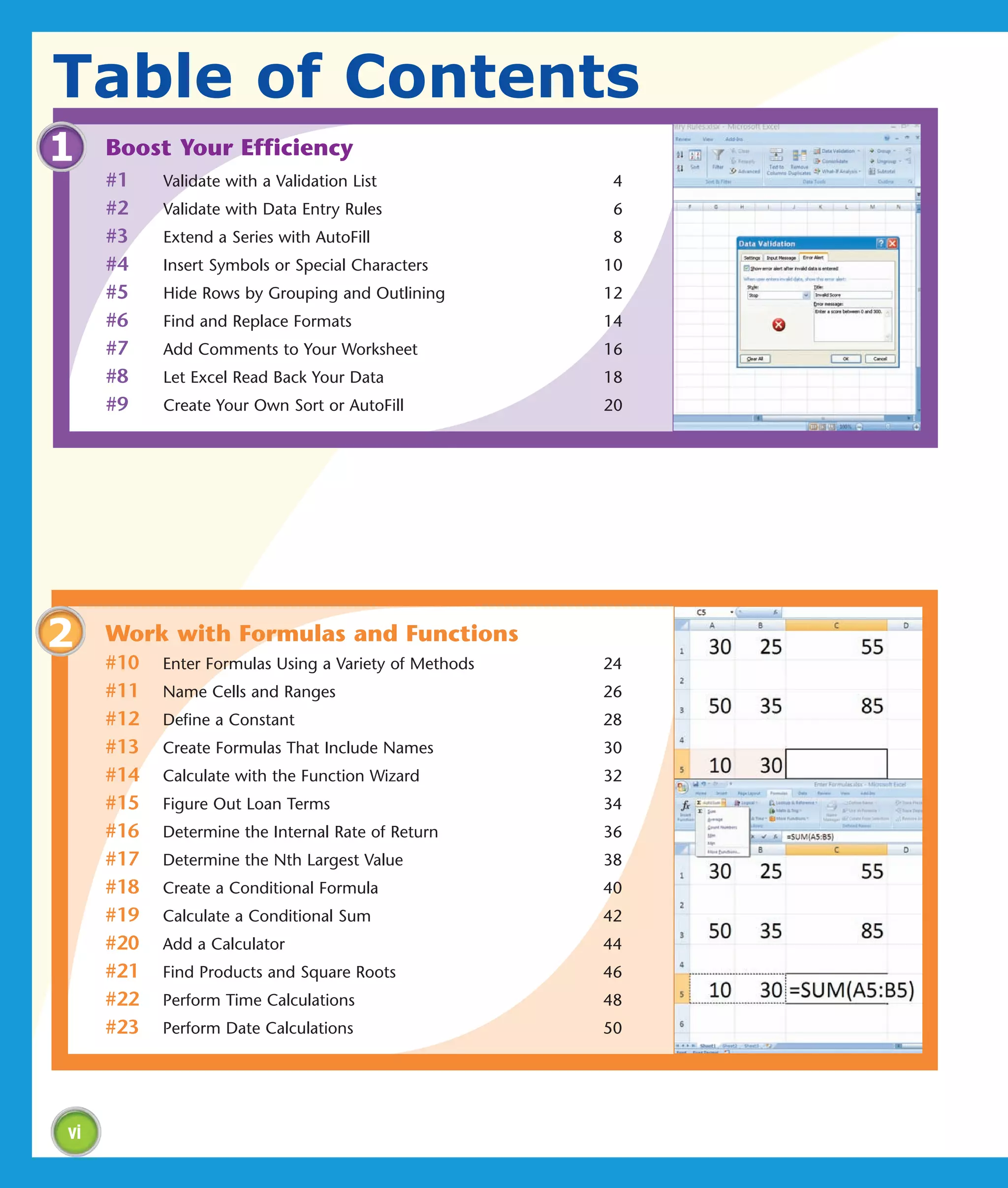

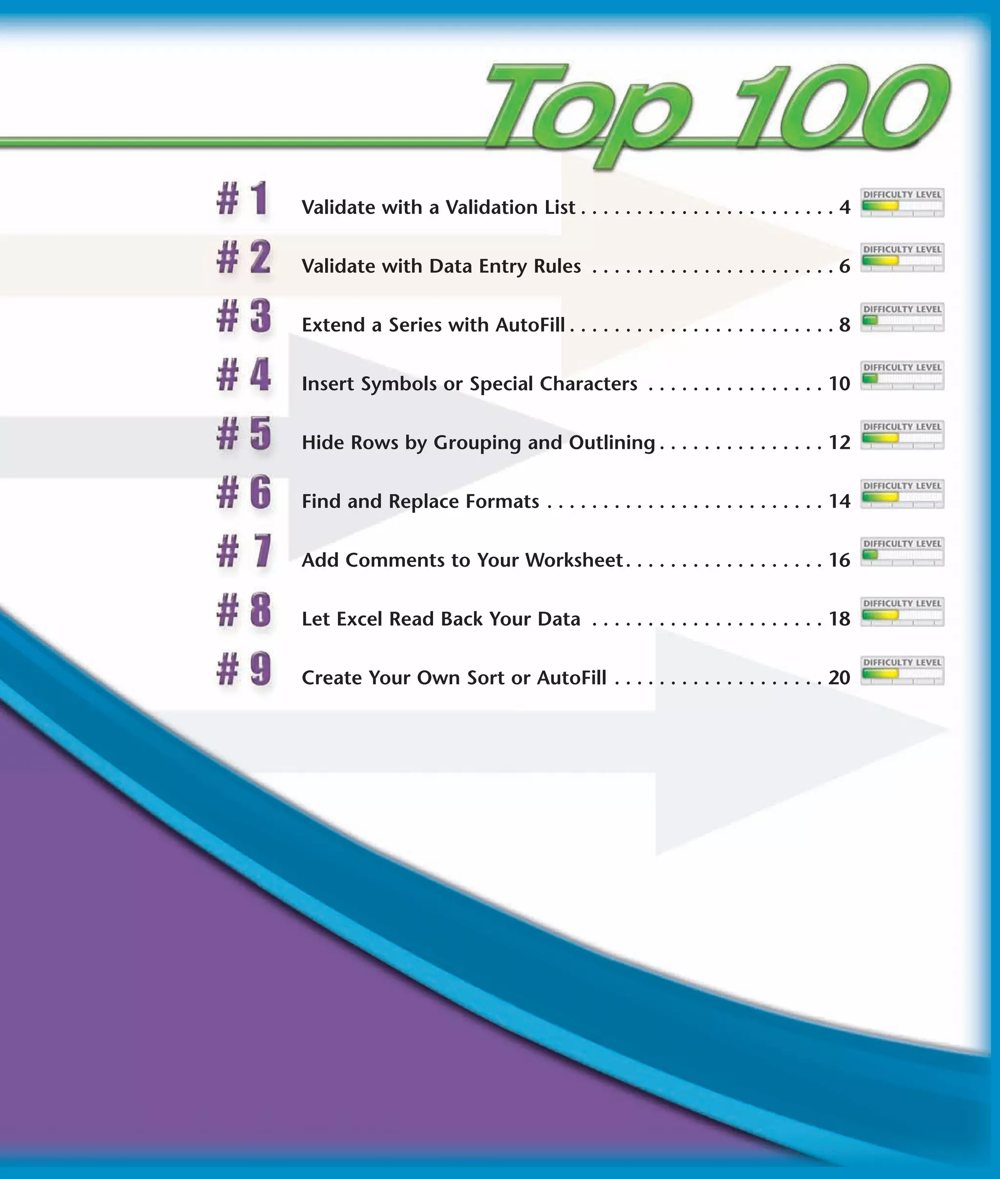
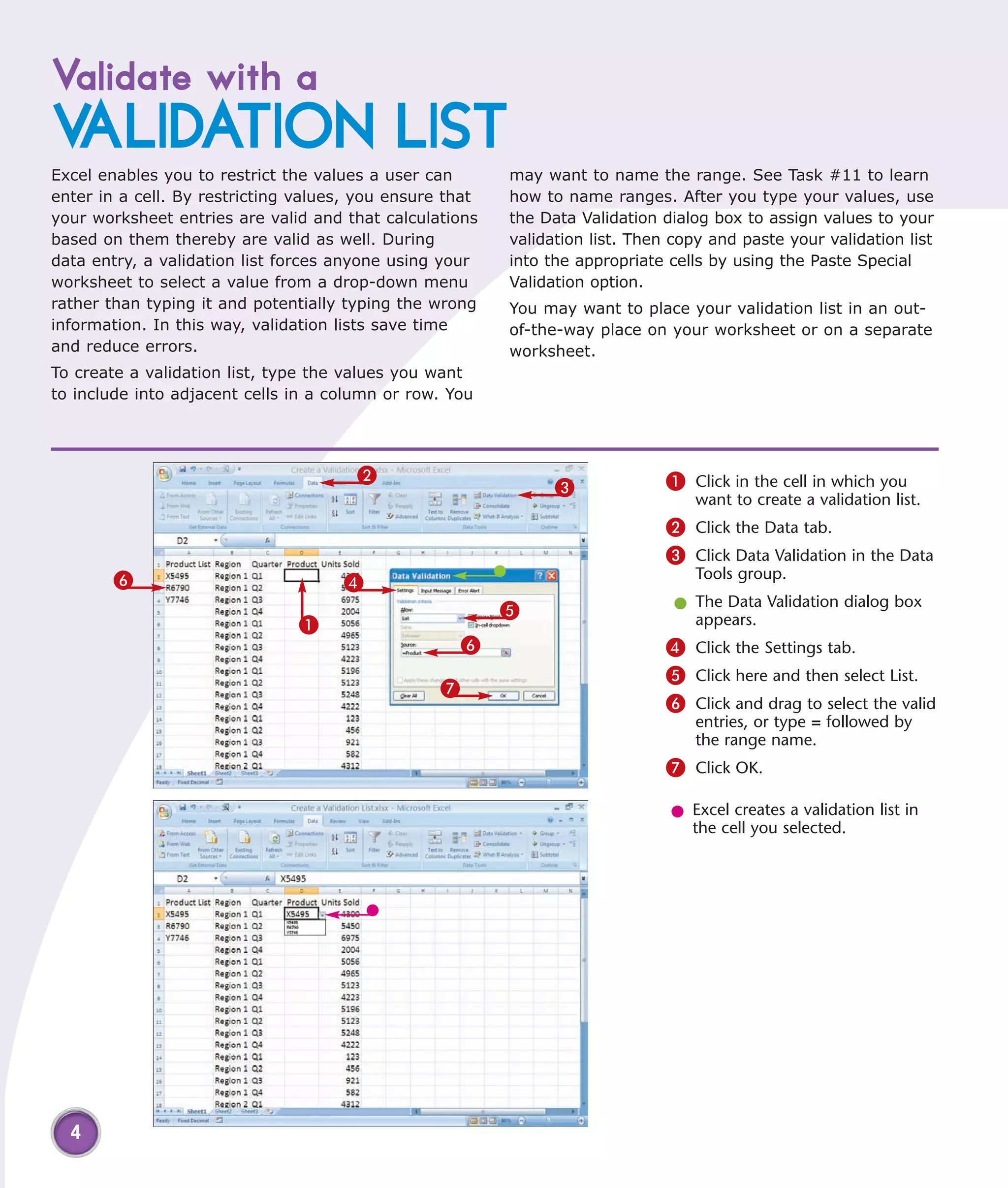
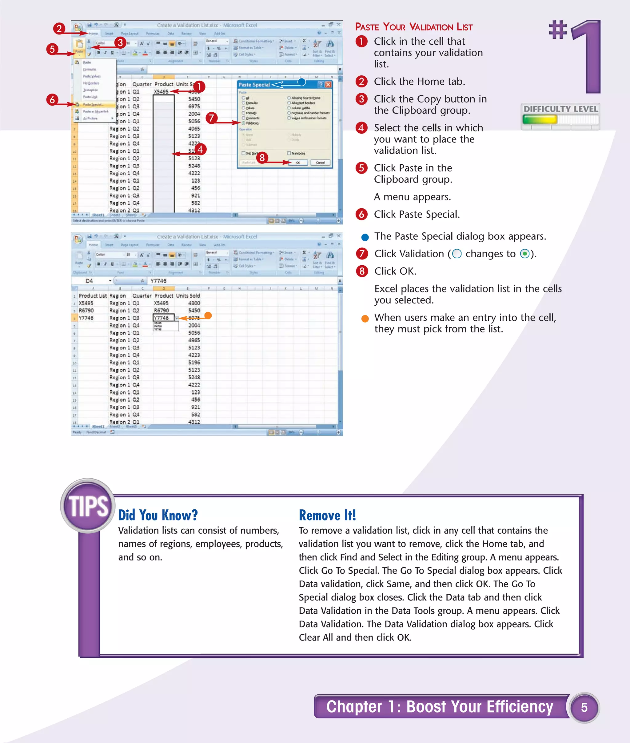
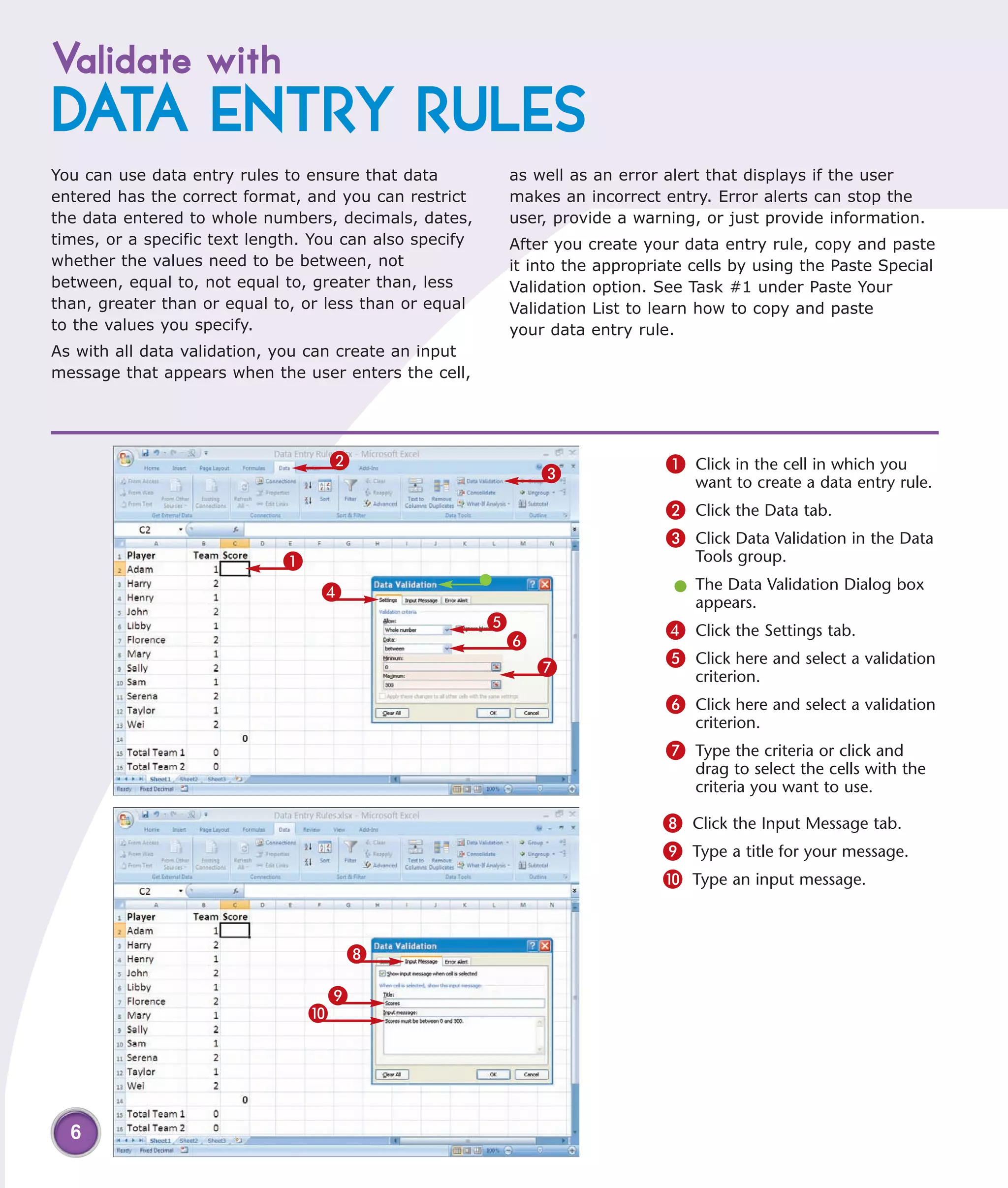
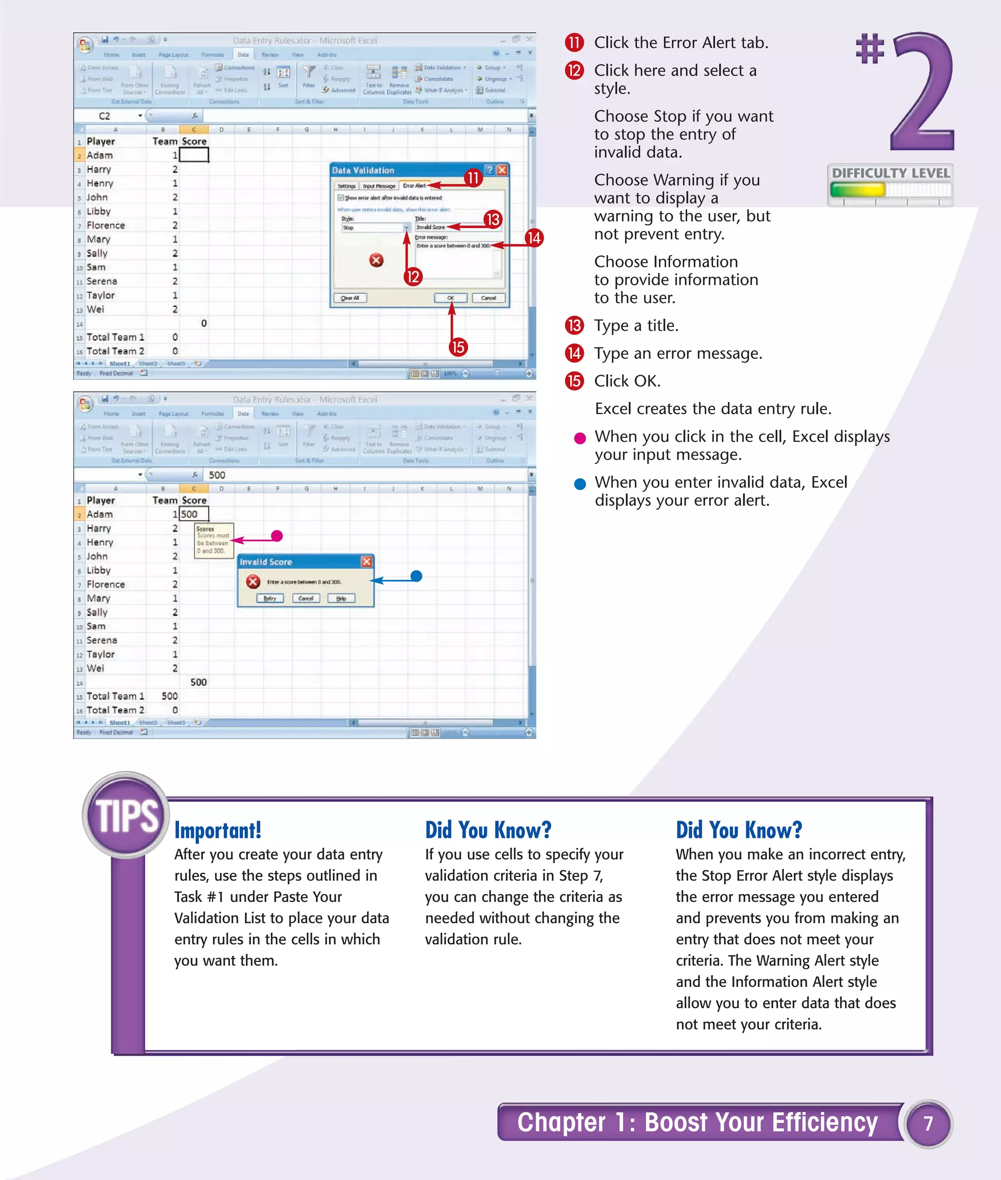
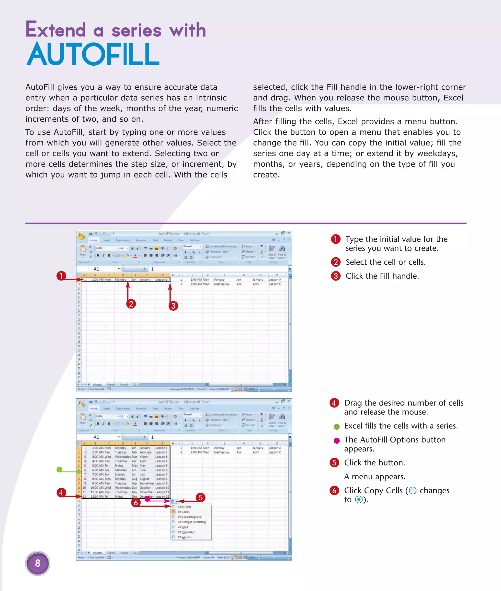
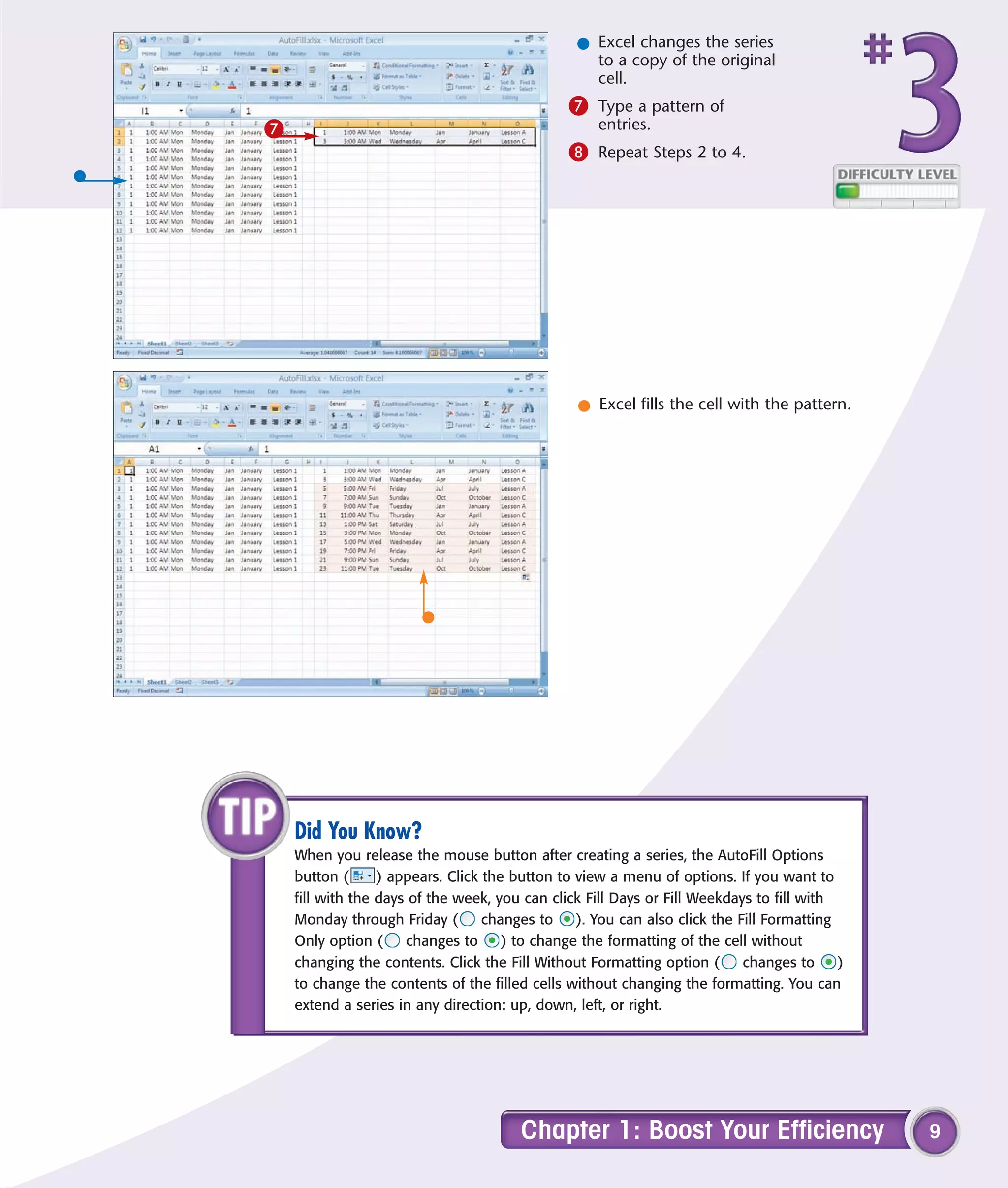
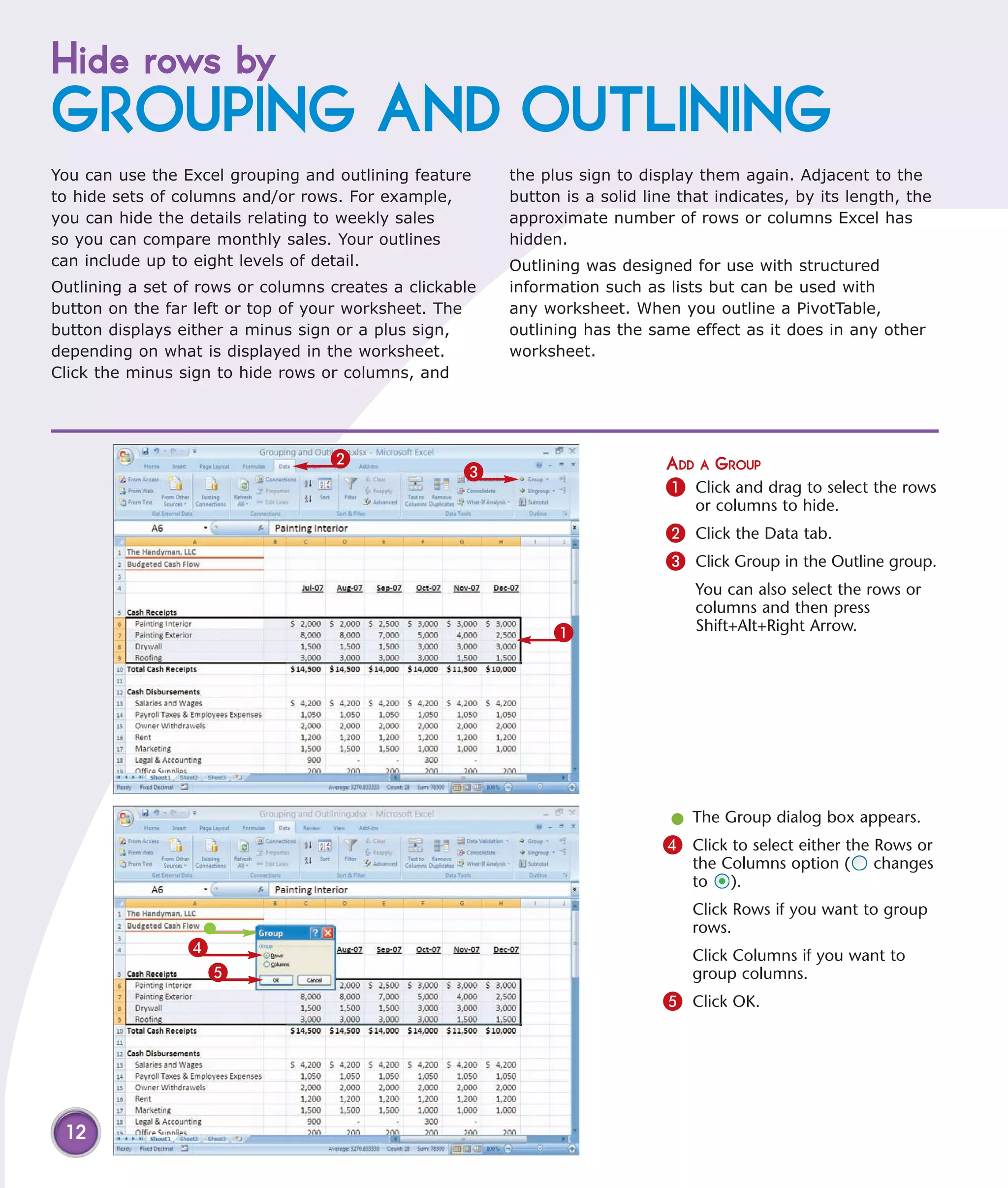
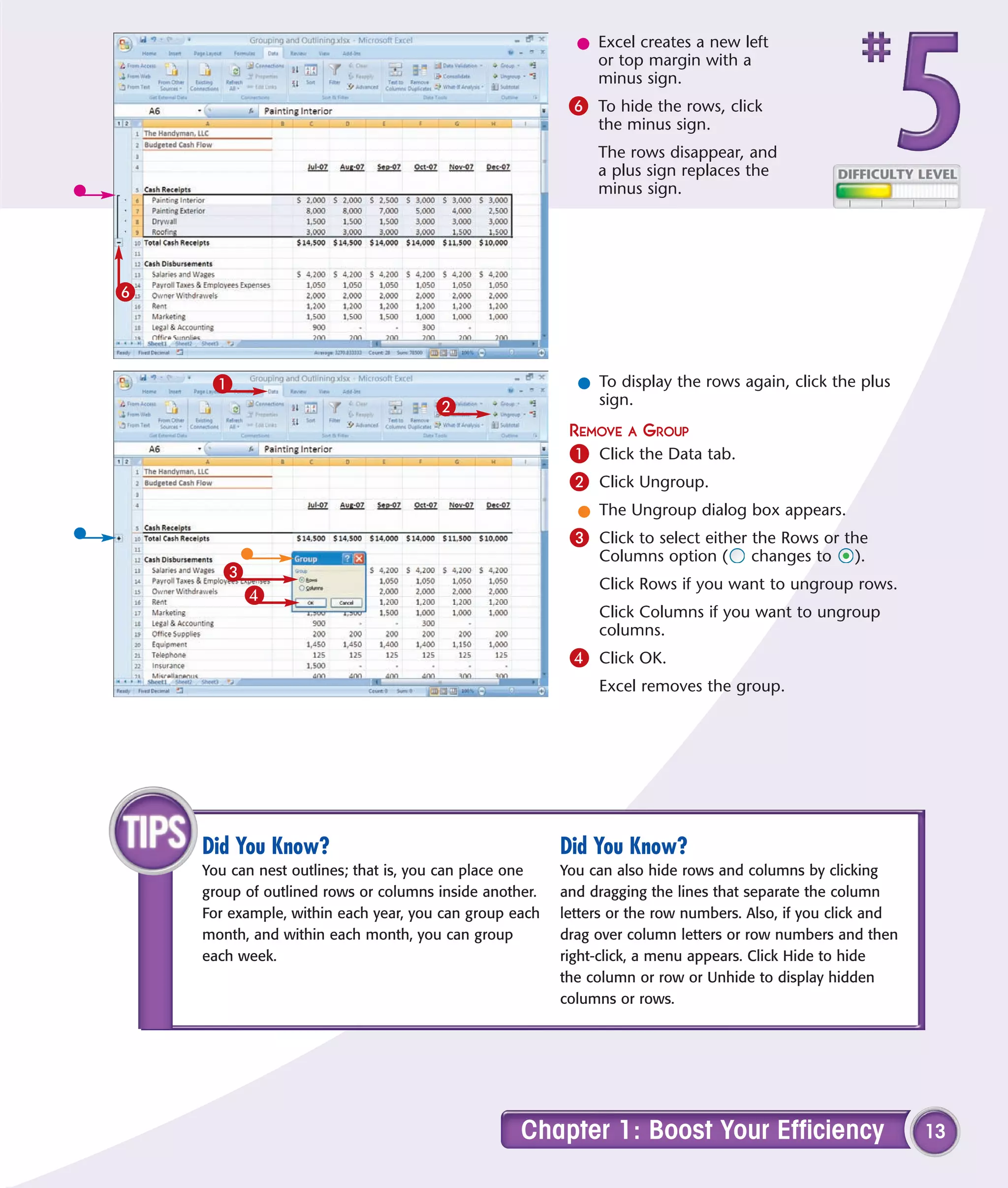
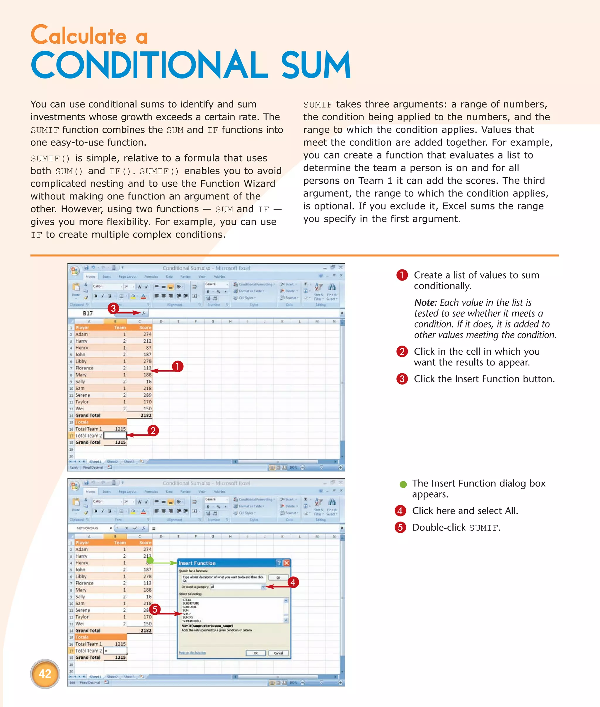


This chapter describes several tips and tricks for boosting efficiency in Excel 2007: 1) Validate data entry with lists or rules to help prevent errors 2) Extend data series automatically using AutoFill to copy patterns 3) Hide rows by outlining or grouping to reduce clutter on worksheets The chapter focuses on streamlining common tasks like data entry, formatting, and organizing worksheets for improved productivity in Excel. Tips include validating inputs, extending series automatically, and hiding unnecessary rows through outlining or grouping.