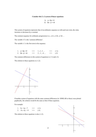
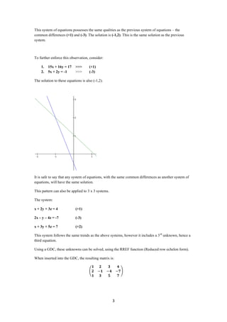
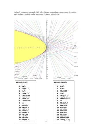
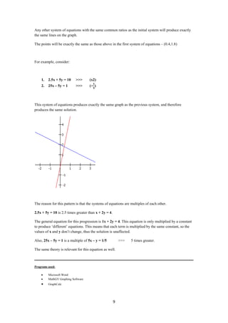
Math Portfolio – HL Type 1


Patterns within systems of linear
           equations


           Year 2012


                1
Consider this 2 x 2 system of linear equations:

                                                  1. x + 2y = 3
                                                  2. 2x – y = -4


This system of equations represents that of an arithmetic sequence as with each new term, the value
increases or decreases by a constant.

The common sequence for arithmetic progressions is a , a+d , a+2d , a+3d …

The variable ‘d’ is the ‘common difference’.

The variable ‘a’ is the first term in the sequence.


    1.   x + 2y = 3         >>>      1,2,3…               >>>      (+1)
    2.   2x - y = -4        >>>      2 , -1 , -4 …        >>>      (-3)

The common differences in this system of equations is (+1) and (-3).

The solution to these equations is (-1,2).


If another system of equations with the same common differences (ie: SIMILAR to these) were plotted
graphically, the solution would be the same as that of these equations.

For example:

    1.   5x + 6y = 7        >>>      (+1)
    2.   -3x - 6y = -9      >>>      (-3)

The solution to these equations is also (-1,2).


                                                      2
This system of equations possesses the same qualities as the previous system of equations – the
common differences (+1) and (-3). The solution is (-1,2). This is the same solution as the previous
system.


To further enforce this observation, consider:

    1.   15x + 16y = 17     >>>      (+1)
    2.   5x + 2y = -1       >>>      (-3)

The solution to these equations is also (-1,2).


It is safe to say that any system of equations, with the same common differences as another system of
equations, will have the same solution.

This pattern can also be applied to 3 x 3 systems.

The system:

x + 2y + 3z = 4             (+1)

2x – y – 4z = -7            (-3)

x + 3y + 5z = 7             (+2)

This system follows the same trends as the above systems, however it includes a 3 rd unknown, hence a
third equation.

Using a GDC, these unknowns can be solved, using the RREF function (Reduced row echelon form).

When inserted into the GDC, the resulting matrix is:


                                                     3
The resulting display (after rref) is –


This means that the variables x, y and z, have an infinite number of solutions.

The equations derived from this matrix mean:

x -1z = -2

y + 2z = 3


In terms of z (which is the common variable in both equations):

x = -2 + z

y = 3 – 2z


These equations >>>                   x + 2y + 3z = 4    can be rearranged in the form z = ax + by + c

                                      2x – y – 4z = -7

                                      x + 3y + 5z = 7


x + 2y + 3z = 4             >>>                3z = -x -2y +4    >>>               z = (-x -2y +4)/3

2x – y – 4z = -7            >>>                -4z = -2x + y -7 >>>                z = (-2x + y -7)/-4

x + 3y + 5z = 7             >>>                5z = -x – 3y +7   >>>               z = (-x – 3y +7)/5


If these equations were plotted graphically, they would produce a 3d graph.


                                                     4
Each plane represents one of the three equations. All three planes meet in a common line. In this case,
the solution is a line of solutions.


Earlier, it was stated that any 2 x 2 system that followed the same trend, and possessed the same
common differences, produced the same solution.

This is the same for 3 x 3 systems.

For example, another 3 x 3 system with the same common differences such as:


Will produce the same graph.

The result (after rrf) is:


This is the same as the previous 3 x 3 system, hence the solutions will be the same, and this will
obviously produce the same 3d graph, hence the same solutions.


___________________________________________________________________________


                                                    5
Consider this 2 x 2 system:

                                                 1. x + 2y = 4
                                                2. 5x – y = 1/5


This system of equations, unlike the previous system, resembles that of a geometric sequence.

In this type of progression, each term is multiplied (or divided) by a constant – known as the ‘common
ratio’.

The general sequence for a geometric progression is a , ar , ar2, ar3 …

The variable ‘r’ is the constant that is multiplied to each term, to produce the following term.

The variable ‘a’ is the first term of the sequence.


    1.   x + 2y = 4         >>>      1,2,4…               >>>     (x2)
    2.   5x – y =           >>>      5 , -1 , …           >>>     (   )

The common ratio in this system of equations are (x2) and (       )


If the equations are written in the form y = ax +b, another pattern is visible.

    1.   x + 2y = 4         >>>      y = (4-x)/2          >>>     y=2– x
    2.   5x – y =           >>>      y = 5x –


The solution to these equations is (0.4,1.8).


Now it is also apparent that a and b themselves are related.


In the first equation, a = , b = 2

b is four times greater than a. The common ratio is 2.


                                                      6
Now, the connection can be perceived.

b is multiplied by the square of the common ratio to give a

           b = a*r2           (Where r = the common ratio).

           b = a*r2           >>>      b = *(2) 2                     >>>   b=2


                            To make it easier to form other equations that follow the same
                            trend, it can be rewritten as:

                                                           y=a–


In the second equation, a = 5 , b =

A similar pattern is visible.

b is one twenty fifth of b. The common ratio is - .

b = a*r2              >>>     b = 5*(- ) 2                 >>>        b=


                                This can also be rewritten to make the pattern easier to see:

                                                           y = bx -


The solution to these equations is (0.4,1.8).


                                                       7
If a family of equations is created, which follow the same trend as the previous systems, the resulting
graph produces a parabola that has been rotated 90 degrees anticlockwise.


   Related to 2-x/2                                               Related to 5x-1/5

        1.    4-x/4                                                    1.    4x-1/4
        2.    3.5-(x/3.5)                                              2.    3x-1/3
        3.    3-x/3                                                    3.    2.5x-1/2.5
        4.    2.5-(x/2.5)                                              4.    2x-1/2
        5.    1.75-x/1.75                                              5.    1.5x-(1/1.5)
        6.    1.5-(x/1.5)                                              6.    1.25x-(1/1.25)
        7.    1.25-x/1.25)                                             7.    x-1
        8.    1-x                                                      8.    0.9x-(1/0.9)
        9.    0.9-x/0.9                                                9.    0.8x-1/0.8
        10.   0.8-(x/0.8)                                              10.   0.7x-1/0.7
        11.   0.7-(x/0.7)                                              11.   0.6x-1/0.6
        12.   0.6-(x/0.6                                               12.   0.5x-1/0.5
        13.   0.5-x/0.5                                                13.   0.3x-1/03
        14.   0.4-x/0.4                                                14.   0.25x-1/0.25
        15.   0.3-(x/0.3)                                              15.   1.15x-(1/1.15)
                                                    8
Any other system of equations with the same common ratios as the initial system will produce exactly
the same lines on the graph.

The points will be exactly the same as those above in the first system of equations – (0.4,1.8)


For example, consider:


    1.   2.5x + 5y = 10    >>>       (x2)
    2.   25x – 5y = 1      >>>       (÷ )


This system of equations produces exactly the same graph as the previous system, and therefore
produces the same solution.


The reason for this pattern is that the systems of equations are multiples of each other.

2.5x + 5y = 10 is 2.5 times greater than x + 2y = 4.

The general equation for this progression is 1x + 2y = 4. This equation is only multiplied by a constant
to produce ‘different’ equations. This means that each term is multiplied by the same constant, so the
values of x and y don’t change, thus the solution is unaffected.

Also, 25x – 5y = 1 is a multiple of 5x – y = 1/5           >>>   5 times greater.

The same theory is relevant for this equation as well.

___________________________________________________________________________________

Programs used:

         Microsoft Word
         MathGV Graphing Software
         GraphCalc


                                                       9

Maths portffolio sequences (2)

  • 1.
    Math Portfolio –HL Type 1 Patterns within systems of linear equations Year 2012 1
  • 2.
    Consider this 2x 2 system of linear equations: 1. x + 2y = 3 2. 2x – y = -4 This system of equations represents that of an arithmetic sequence as with each new term, the value increases or decreases by a constant. The common sequence for arithmetic progressions is a , a+d , a+2d , a+3d … The variable ‘d’ is the ‘common difference’. The variable ‘a’ is the first term in the sequence. 1. x + 2y = 3 >>> 1,2,3… >>> (+1) 2. 2x - y = -4 >>> 2 , -1 , -4 … >>> (-3) The common differences in this system of equations is (+1) and (-3). The solution to these equations is (-1,2). If another system of equations with the same common differences (ie: SIMILAR to these) were plotted graphically, the solution would be the same as that of these equations. For example: 1. 5x + 6y = 7 >>> (+1) 2. -3x - 6y = -9 >>> (-3) The solution to these equations is also (-1,2). 2
  • 3.
    This system ofequations possesses the same qualities as the previous system of equations – the common differences (+1) and (-3). The solution is (-1,2). This is the same solution as the previous system. To further enforce this observation, consider: 1. 15x + 16y = 17 >>> (+1) 2. 5x + 2y = -1 >>> (-3) The solution to these equations is also (-1,2). It is safe to say that any system of equations, with the same common differences as another system of equations, will have the same solution. This pattern can also be applied to 3 x 3 systems. The system: x + 2y + 3z = 4 (+1) 2x – y – 4z = -7 (-3) x + 3y + 5z = 7 (+2) This system follows the same trends as the above systems, however it includes a 3 rd unknown, hence a third equation. Using a GDC, these unknowns can be solved, using the RREF function (Reduced row echelon form). When inserted into the GDC, the resulting matrix is: 3
  • 4.
    The resulting display(after rref) is – This means that the variables x, y and z, have an infinite number of solutions. The equations derived from this matrix mean: x -1z = -2 y + 2z = 3 In terms of z (which is the common variable in both equations): x = -2 + z y = 3 – 2z These equations >>> x + 2y + 3z = 4 can be rearranged in the form z = ax + by + c 2x – y – 4z = -7 x + 3y + 5z = 7 x + 2y + 3z = 4 >>> 3z = -x -2y +4 >>> z = (-x -2y +4)/3 2x – y – 4z = -7 >>> -4z = -2x + y -7 >>> z = (-2x + y -7)/-4 x + 3y + 5z = 7 >>> 5z = -x – 3y +7 >>> z = (-x – 3y +7)/5 If these equations were plotted graphically, they would produce a 3d graph. 4
  • 5.
    Each plane representsone of the three equations. All three planes meet in a common line. In this case, the solution is a line of solutions. Earlier, it was stated that any 2 x 2 system that followed the same trend, and possessed the same common differences, produced the same solution. This is the same for 3 x 3 systems. For example, another 3 x 3 system with the same common differences such as: Will produce the same graph. The result (after rrf) is: This is the same as the previous 3 x 3 system, hence the solutions will be the same, and this will obviously produce the same 3d graph, hence the same solutions. ___________________________________________________________________________ 5
  • 6.
    Consider this 2x 2 system: 1. x + 2y = 4 2. 5x – y = 1/5 This system of equations, unlike the previous system, resembles that of a geometric sequence. In this type of progression, each term is multiplied (or divided) by a constant – known as the ‘common ratio’. The general sequence for a geometric progression is a , ar , ar2, ar3 … The variable ‘r’ is the constant that is multiplied to each term, to produce the following term. The variable ‘a’ is the first term of the sequence. 1. x + 2y = 4 >>> 1,2,4… >>> (x2) 2. 5x – y = >>> 5 , -1 , … >>> ( ) The common ratio in this system of equations are (x2) and ( ) If the equations are written in the form y = ax +b, another pattern is visible. 1. x + 2y = 4 >>> y = (4-x)/2 >>> y=2– x 2. 5x – y = >>> y = 5x – The solution to these equations is (0.4,1.8). Now it is also apparent that a and b themselves are related. In the first equation, a = , b = 2 b is four times greater than a. The common ratio is 2. 6
  • 7.
    Now, the connectioncan be perceived. b is multiplied by the square of the common ratio to give a b = a*r2 (Where r = the common ratio). b = a*r2 >>> b = *(2) 2 >>> b=2 To make it easier to form other equations that follow the same trend, it can be rewritten as: y=a– In the second equation, a = 5 , b = A similar pattern is visible. b is one twenty fifth of b. The common ratio is - . b = a*r2 >>> b = 5*(- ) 2 >>> b= This can also be rewritten to make the pattern easier to see: y = bx - The solution to these equations is (0.4,1.8). 7
  • 8.
    If a familyof equations is created, which follow the same trend as the previous systems, the resulting graph produces a parabola that has been rotated 90 degrees anticlockwise. Related to 2-x/2 Related to 5x-1/5 1. 4-x/4 1. 4x-1/4 2. 3.5-(x/3.5) 2. 3x-1/3 3. 3-x/3 3. 2.5x-1/2.5 4. 2.5-(x/2.5) 4. 2x-1/2 5. 1.75-x/1.75 5. 1.5x-(1/1.5) 6. 1.5-(x/1.5) 6. 1.25x-(1/1.25) 7. 1.25-x/1.25) 7. x-1 8. 1-x 8. 0.9x-(1/0.9) 9. 0.9-x/0.9 9. 0.8x-1/0.8 10. 0.8-(x/0.8) 10. 0.7x-1/0.7 11. 0.7-(x/0.7) 11. 0.6x-1/0.6 12. 0.6-(x/0.6 12. 0.5x-1/0.5 13. 0.5-x/0.5 13. 0.3x-1/03 14. 0.4-x/0.4 14. 0.25x-1/0.25 15. 0.3-(x/0.3) 15. 1.15x-(1/1.15) 8
  • 9.
    Any other systemof equations with the same common ratios as the initial system will produce exactly the same lines on the graph. The points will be exactly the same as those above in the first system of equations – (0.4,1.8) For example, consider: 1. 2.5x + 5y = 10 >>> (x2) 2. 25x – 5y = 1 >>> (÷ ) This system of equations produces exactly the same graph as the previous system, and therefore produces the same solution. The reason for this pattern is that the systems of equations are multiples of each other. 2.5x + 5y = 10 is 2.5 times greater than x + 2y = 4. The general equation for this progression is 1x + 2y = 4. This equation is only multiplied by a constant to produce ‘different’ equations. This means that each term is multiplied by the same constant, so the values of x and y don’t change, thus the solution is unaffected. Also, 25x – 5y = 1 is a multiple of 5x – y = 1/5 >>> 5 times greater. The same theory is relevant for this equation as well. ___________________________________________________________________________________ Programs used: Microsoft Word MathGV Graphing Software GraphCalc 9