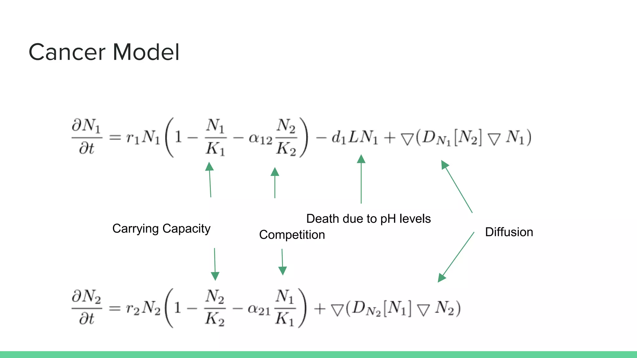
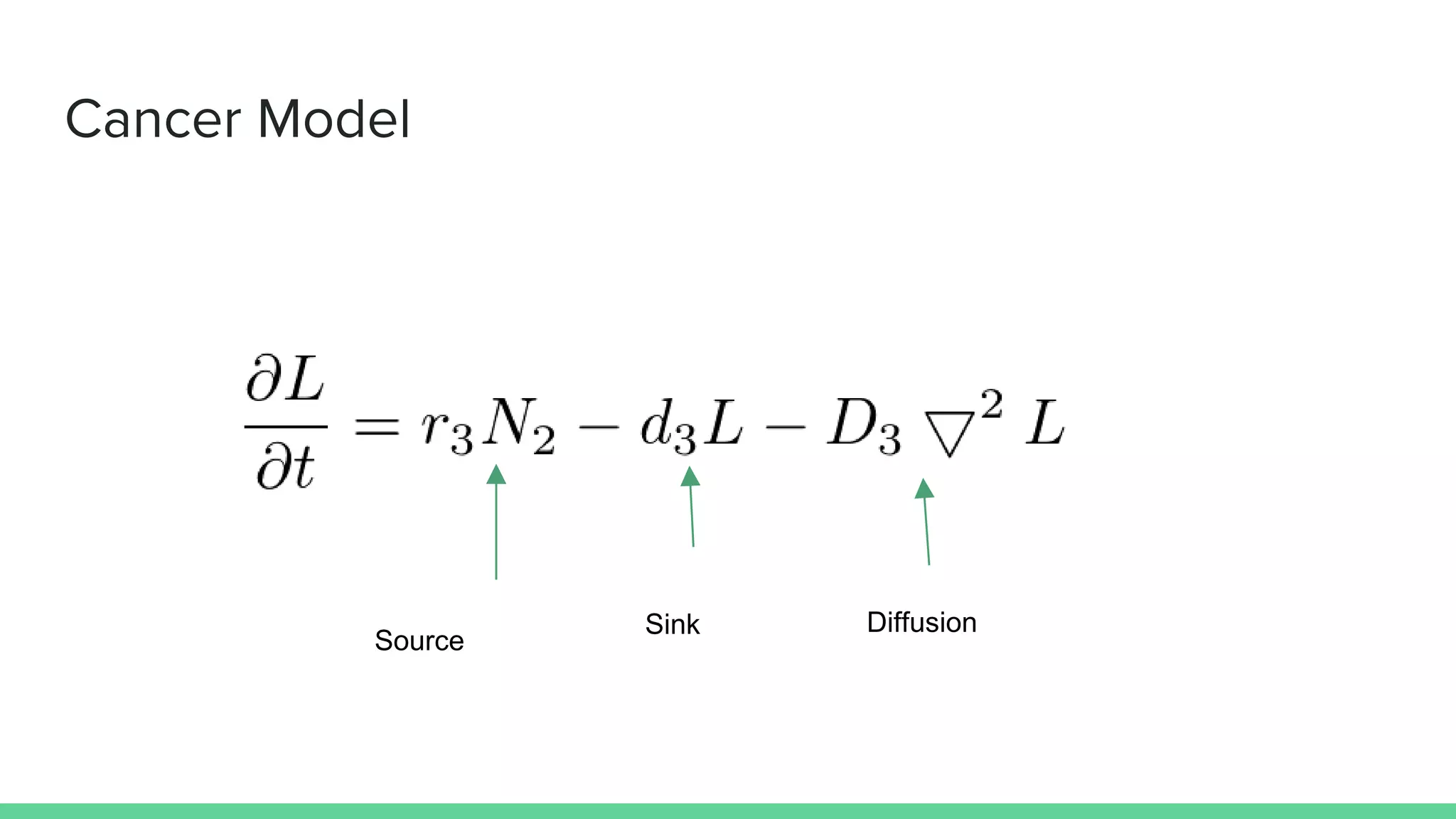
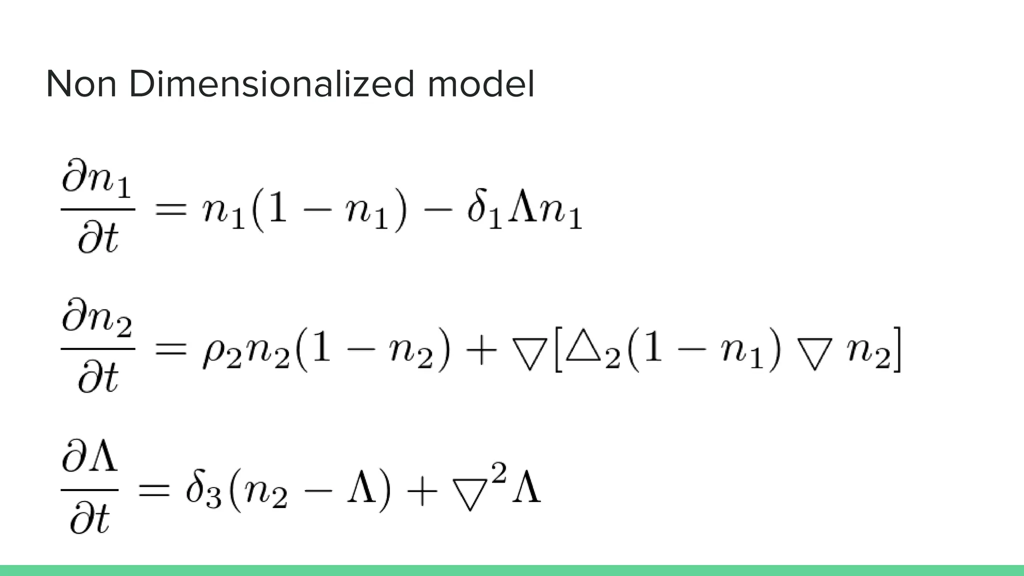
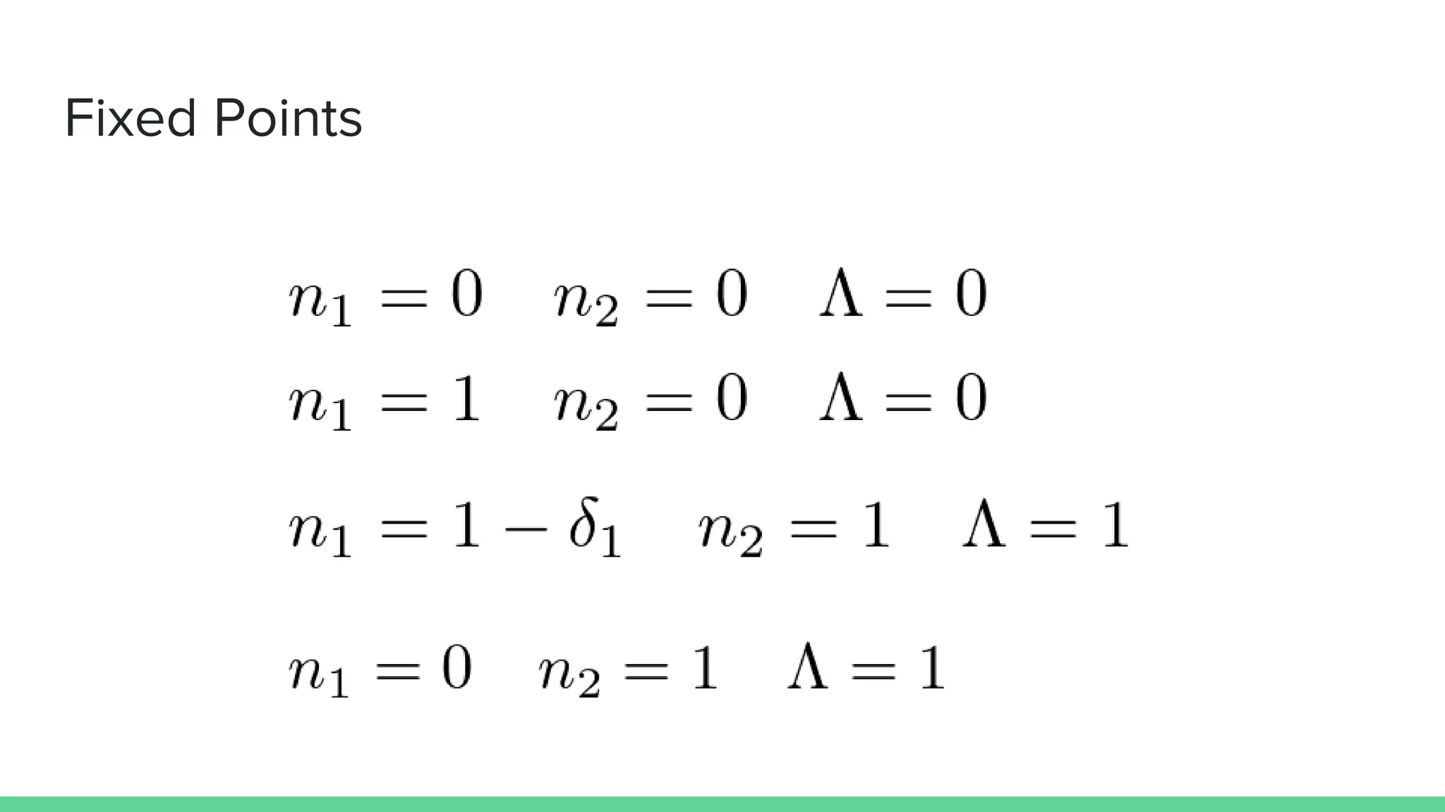
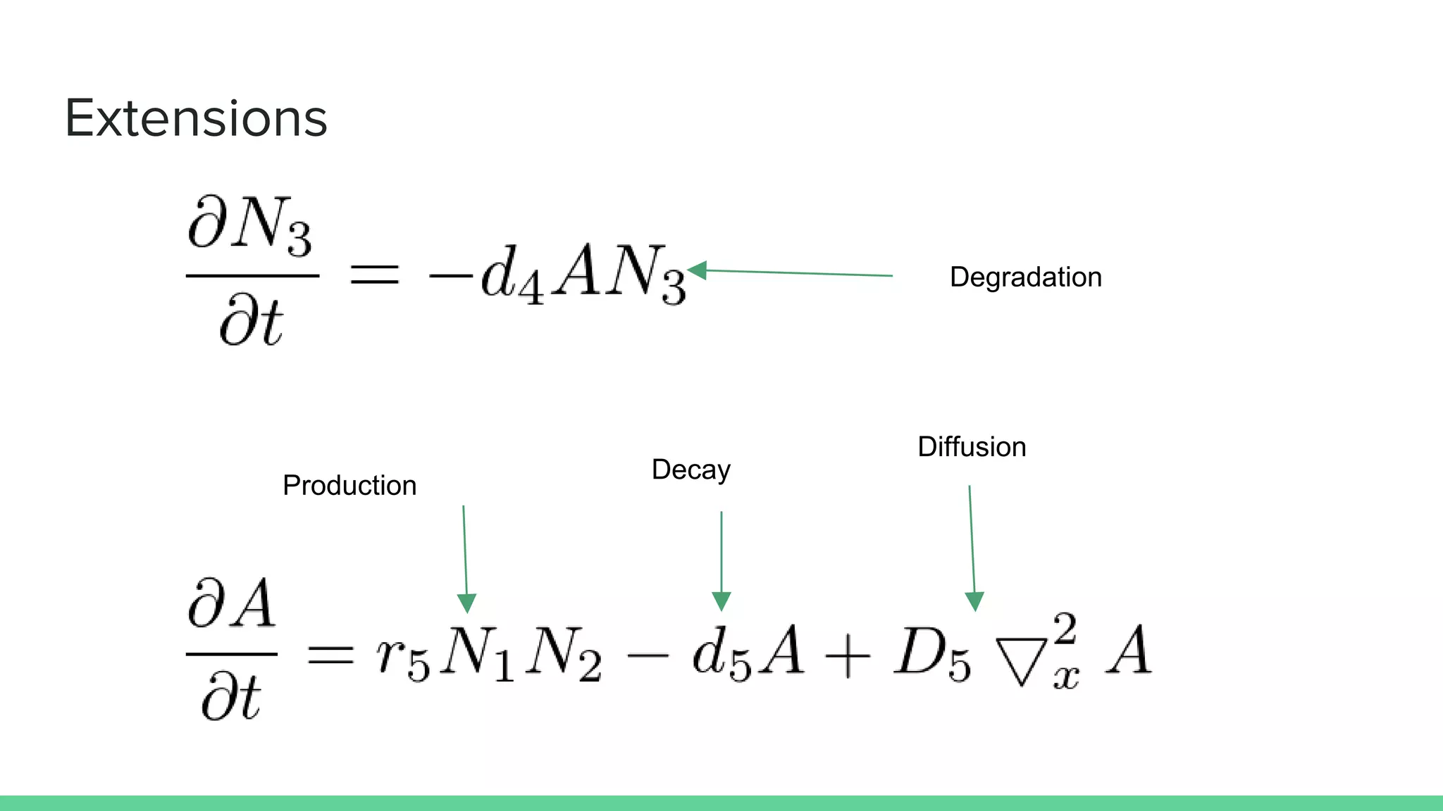
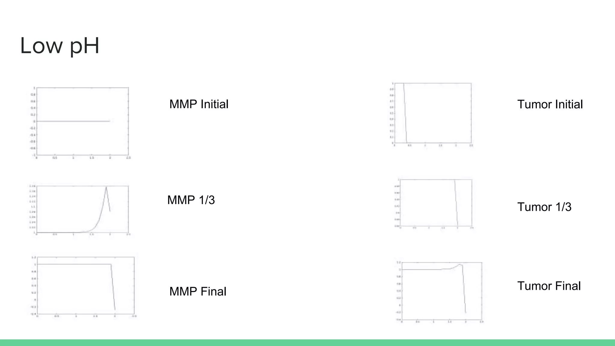
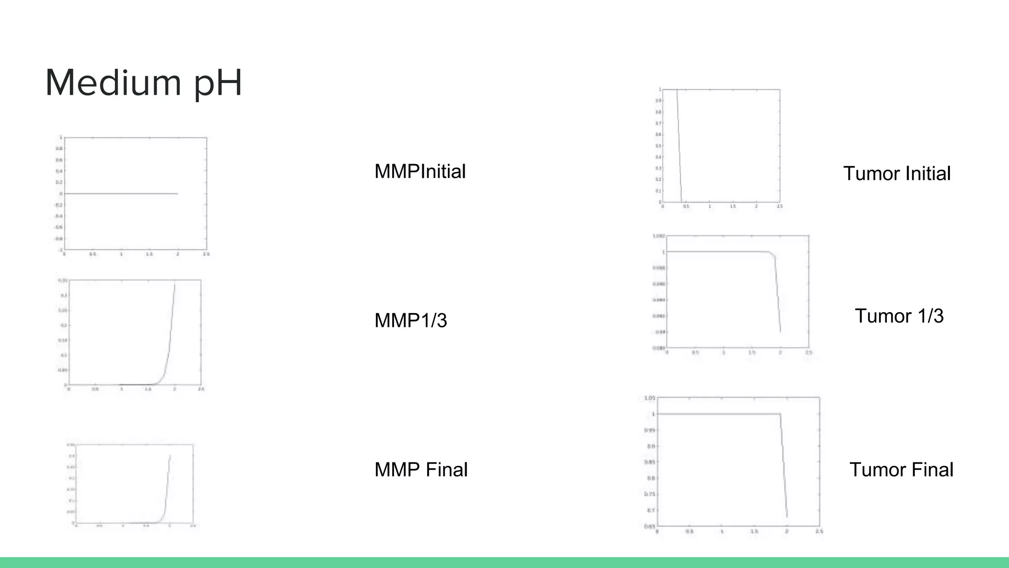
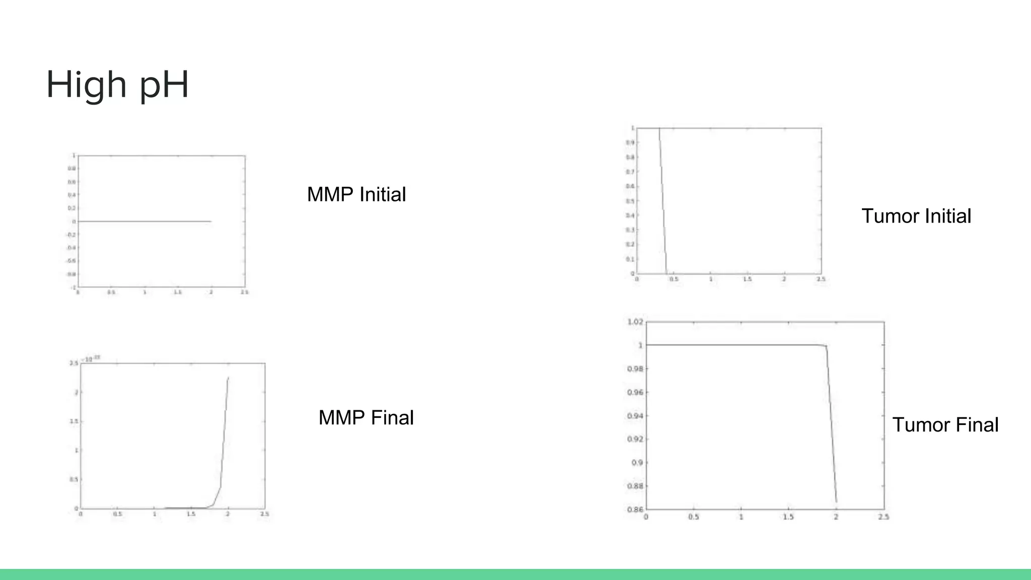
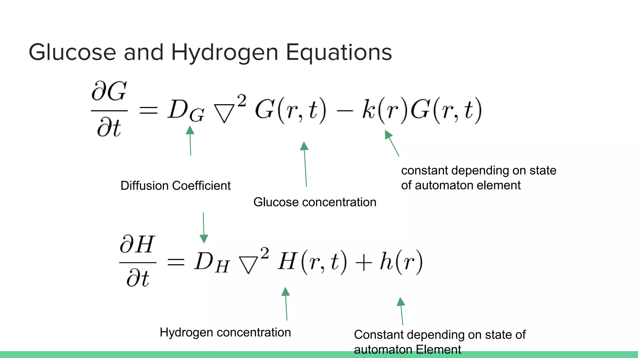
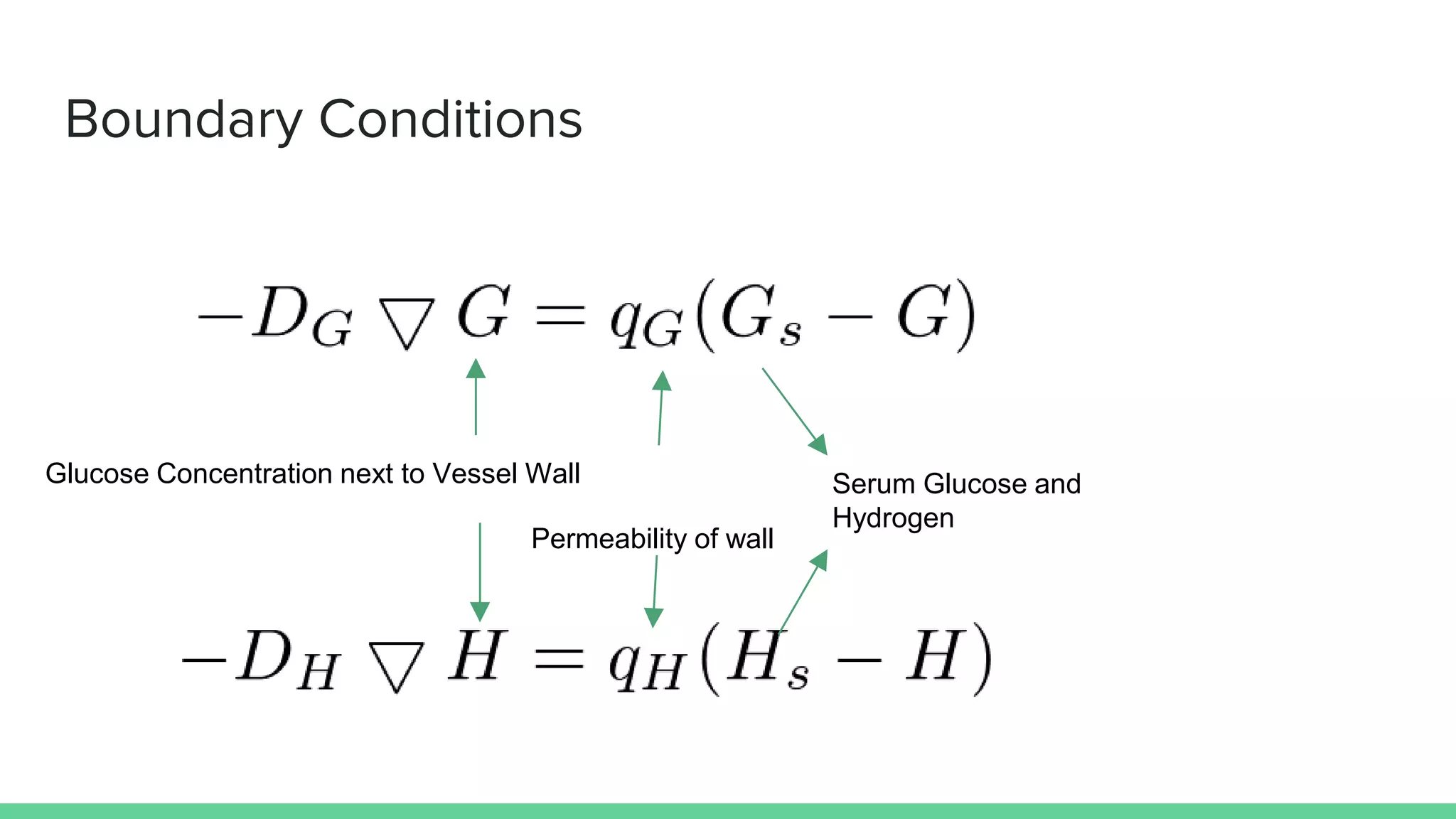
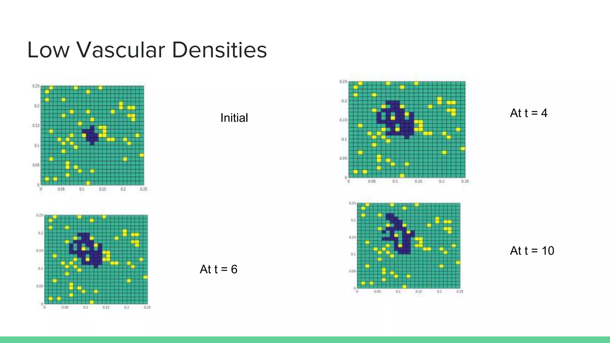
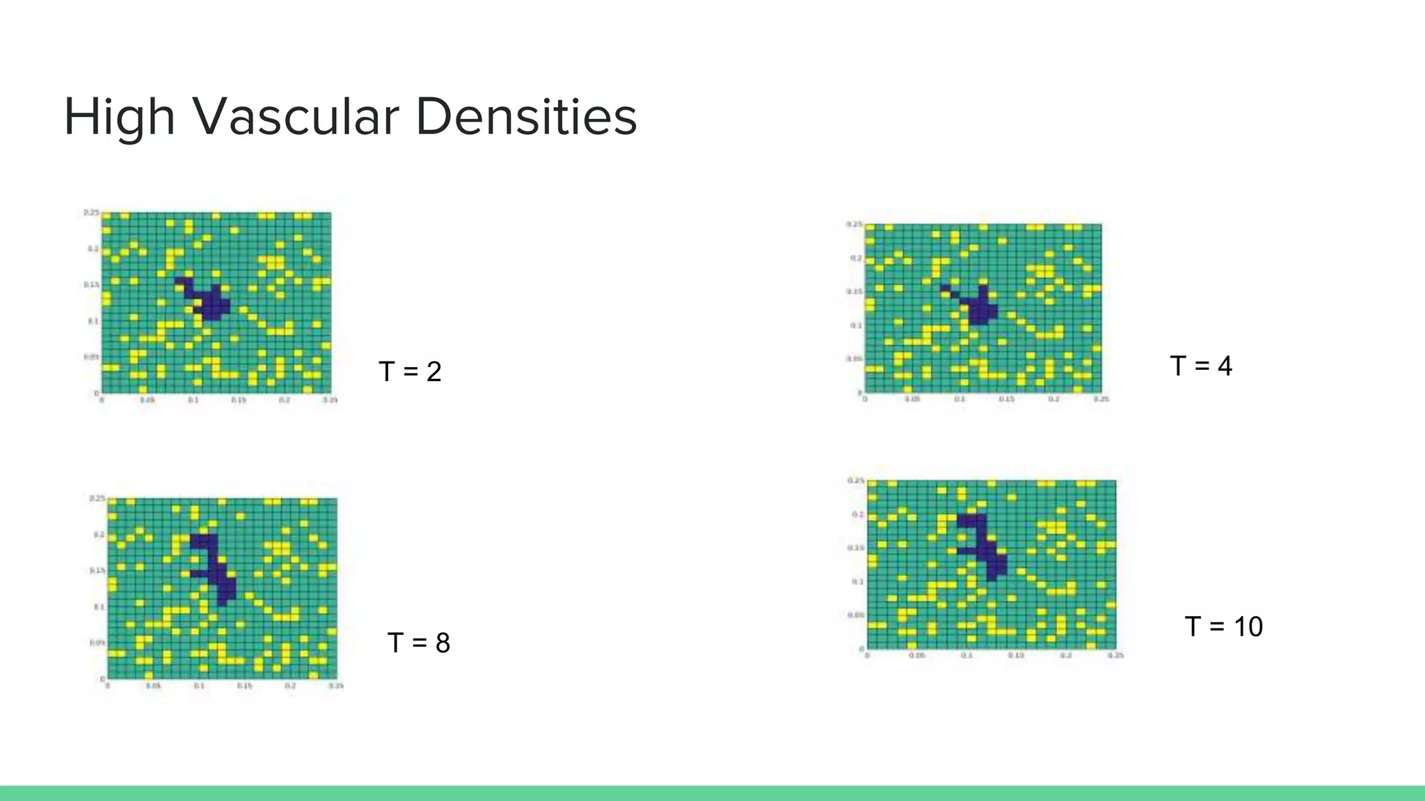
Mathematical Models of
Tumor Invasion
Sean Davis
Overview
Goal: Examine how a mathematical idea, matures and understands natural
phenomena, aside from physics
Cellular Automata / Discrete and Local Cancer Models
Reaction Diffusion Equations / Continuous Global Cancer Models
Reaction Diffusion Equations
Mathematical framework for describing how entities interact as they change in time
and space
Applications:
Embryology
Tumors
Pattern Development of Mollusc Shells
Epidemic Models
General Equations
Kinetics
Acceleration in x-direction
Acceleration in y-direction
Diffusion Coefficients
Linear Stability
Diffusion is a form of stabilisation
Diffusion - Driven Instability
Grasshoppers and Fire
Non-Dimensionalized Equations
Diffusion Ratio
Method of Lines
Simulation Results
Initial
Half Way
Quarter way
At t = 10
Cancer Model
Key Insight: Transformation of Tumors - Makes more Acid
Aligned with Empirical Studies (Accuracy)
Reaction Diffusion
Population Density
Predator - Prey
Predator Prey Models
Growth due to birth
Death due to predations
Growth due to predation Death
Population Density
Cancer Model
Carrying Capacity Competition
Death due to pH levels
Diffusion
Cancer Model
Source
Sink Diffusion
Non Dimensionalized model
Fixed Points
Extensions
Degradation
Production
Decay
Diffusion
Low pH
MMP Initial
MMP 1/3
MMP Final
Tumor Initial
Tumor 1/3
Tumor Final
Medium pH
MMPInitial
MMP Final
Tumor Initial
Tumor Final
MMP1/3 Tumor 1/3
High pH
MMP Initial
MMP Final Tumor Final
Tumor Initial
Cellular Automata
What happens when there aren’t very many cells
Can’t use continuous global model
Instead compute cells individually
States
Normal (and Quiescent Normal)
Tumor (and Quiescent Tumor)
Micro-Vessel
Vacant
Rules
Each Automaton Element is placed on an (N x N) Grid.
If the element is a Tumor or a Normal Cell and the pH are above a min they live
If it is also above a “reproduction threshold” then they have the oppurunity to
reproduce
Provided one of their neighbours have enough glucose
Glucose and Hydrogen Equations
Hydrogen concentration Constant depending on state of
automaton Element
Diffusion Coefficient
Glucose concentration
constant depending on state
of automaton element
Boundary Conditions
Glucose Concentration next to Vessel Wall
Permeability of wall
Serum Glucose and
Hydrogen
Low Vascular Densities
Initial At t = 4
At t = 6
At t = 10
High Vascular Densities
T = 2 T = 4
T = 8
T = 10
Questions?
Bibliography
AALPEN A. PATEL, EDWARD T. GAWLINSKI, SUSAN K. LEMIEUX, ROBERT A. GATENBY, A Cellular Automaton Model of Early Tumor Growth and
Invasion: The Effects of Native Tissue Vascularity and Increased Anaerobic Tumor Metabolism, Journal of Theoretical Biology, Volume 213, Issue 3, 7 December
2001, Pages 315-331, ISSN 0022-5193, http://dx.doi.org/10.1006/jtbi.2001.2385.
Boyce, William E. and DiPrima Richard C. Elementary Differential Equations. 9th Edition. John Wiley & Sons Inc. 2009. Print
Burden Richard L Faire J. Douglase. Numerical Analysis 34d Edition. Boston: PWS Publishers, 1981. Print.
de Vries Gerda, Hillen Thomas, Lewis Mark, Johannes Muller, Schonfisch Birgitt. A Course in Mathematical Biology: Quantitative modeling with 1
Mathematical and Computational Methods. Society for Industrial and Applied Mathematics, 2006, Print.
Martin, Natasha K. et al. “Tumour-Stromal Interactions in Acid-Mediated Invasion: A Mathematical Model.” Journal of theoretical biology 267.3 (2010): 461–
470. PMC. Web. 6 Dec. 2015.
Murray J.D. Mathematical Biology Second, Corrected Edition. Springer, 1991
Gatenby, Robert A. and Gawlinski Edward T. “A Reaction-Diffusion Model of Cancer Invasion. Cancer Research 56 (1996): 5745-5753 (Web) Accessed
December 5th 2015.

Mathematical Models of Tumor Invasion

Editor's Notes

  • #3 Reaction Diffusion Equations: Combined with predator - prey models and population models give a good understanding of cancer possible leading to better treatments
  • #4 Each application as inhibitor and activator where inhibitor stops the activator and the activator drives the inhibitor (to get a feedback mechanism) Reaction Diffusion: Reaction - how the two entities react Diffusion - how the entity spreads through space
  • #5 English Translation: The rate at which A changes in time is equal to the change as a result of an interaction with B and the way it is accelerating in a spatial direction (either one or two dimensional, not necessarily cartesian) Spatial Variation and Laplacing operator: the way it changes in space Diffusion Co-efficents: the diffusivity of the space where the entities lie. How easily can they move around?
  • #6 Stability: Small changes in the system do not create a big effect Unstable systems tend to want to become stable ones Diffusion and Stabilisation: If the entity is spread throughout the system, in its in a state of equilibrium and so will not want to change Diffusion Driven Instability: Instability in the presence of diffusion but not when the equation is only time dependent Grasshopper and Fire: Grashoopers sweat putting out the fire They must be faster What happens when they the fire is spread randomly?
  • #7 Non - dimensionalization: eliminate units to make the mathematics less cumbersome (units come out naturally from the equations). d - ratio of Db to Da (want it large and positive for diffusion driven instability) gamma - ratio of some length and some constant in the kinetics, to Da. Boundary Conditions: Only handle a finite domain, so there is some boundary. need a way to describe how entities move beyond boundary Flux: Mathematical description of how it moves beyond the boundaries. Here we have zero-flux: so no crossing of the bounaries
  • #8 Method of Lines: discretize along two dimensions, (in this case the space ones) and are left with an Ordinary Differential Equation Discretize: breaking a continous element into dicrete components ODE’s: Equations, much like what i’ve been describing except, its only worred about how things change with respect to one of their variables Runge Kutta: We know the right of change, so we know the direction of the curve, just have to plot points in that direction a = 0.2 b = 2.0
  • #10 Based on the hypothesis that: As tissues are transformed into tumor tissue, they are transformed into a primitive methods of absorbing food, which produces appropriate acid levels for tumors and inappropriate acid levels for normal cells
  • #11 Explain how model is derived. Absence of a predator prey just increases Absence of Prey predator dies off. In our model, normal cells are the prey and the tumor cells are the predator.
  • #12 As u approaches 1, where u is a fraction of its carrying capacity, then the change becomes more and more dependent on space.
  • #13 N1 - density of normal cells N2 - density of tumor cells L - concentration of hydrogen ions
  • #15 simplifying assumption: Normal cells do not diffuse throughout the system. This is ok since we are primarily concerned with how the tumor cells are invading
  • #16 Fixed Points: Where no change happens important for the dynamics FP1: Unconditionally unstable trivial absence of everything FP2: Healthy tissue at its carrying capacity, absence of tumor cells/ FP3: tumor tissue at its carrying capacity, normal cells at a diminished level. Conditionally stable delta1 < 1. FP4: tumor tissue at carrying capacity, killed off all normal cells. What this means is that once a tumor is introduced beside one section it will grow into areas that have either FP1 or FP2, as small perturbations cause those fixed points to grow towards 3 or 4.
  • #17 Gatenby’s model is all well and good but it does not account for the ECM (the other stuff around the cells). Matrix Metalloproteinases (MMP): enzymes that degrade the ECM.
  • #18 Simulation Results with low Tumor Agression MMPstopping Tumor Progression Initial Conditions: tumors placed in a small area healthy tissue at carrying capacity everywhere tumor is not hydrogen ions are at zero MMP at carrying capacity Active MMP non-existent. Np-flux boundary conditions
  • #19 Simulation results with Higher Tumor Agression Lack of MMP -easier proliferation of Tumors.
  • #21 Cellular Auomata: Is a mathematical framework for studying systems (mainly through simulation) where each element is a set containing: Neighbours State Local rule for updating based on the neighbours and its curretn state
  • #23 For me N = 25 Spread microvessels randomly throughout the Grid Make a small Tumor disc in the middle For me had a radius of 2 Neighbours: one above, one to the left, one below, one to the right Neighbours wrap around (Periodic Boundary Conditions)
  • #24 Periodic Boundary Conditions Boundary Conditions at the cell wall Initial Condition: Uniform pH of 7.2 Glucose randomly between 2.5 and 5.0 (the min. and maximum levels)
  • #25 Boundary Conditions: Zero - Flux.
  • #26 How simulation works: Keeps track of the glucose and hydrogen concentrations in a seperate vector Keeps track of the grid of cells After the concentrations are updated: Goes through the cells and applies the rules to each cell 25x 25 grid (about 10 hours to complete) Tumor grows, some of it dies off, overall getting bigger This picture not necessarily realistic, but does give a good idea on how it works.