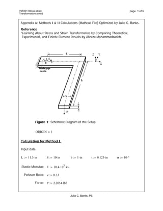
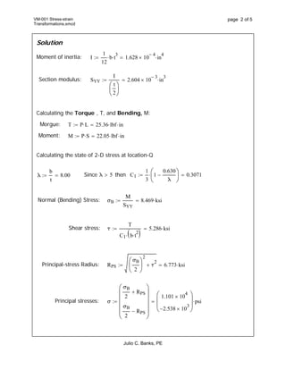
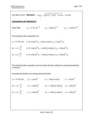
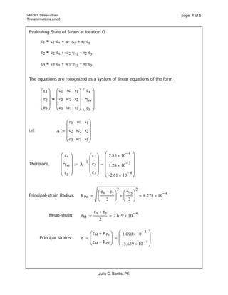
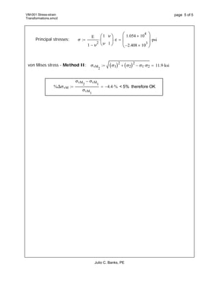
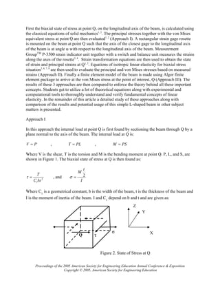
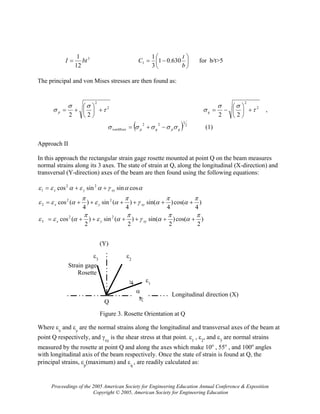
VM-001 Stress-strain
Transformations.xmcd
page 1 of 5
Appendix A: Methods I & II Calculations (Mathcad File) Optimized by Julio C. Banks.
Reference
"Learning About Stress and Strain Transformatios by Comparing Theoretical,
Experimental, and Fininte Element Resutls by Alireza Mohammadzadeh.
Figure 1: Schematic Diagram of the Setup
ORIGIN 1
Calculation for Method I
Input data
L 11.5 in S 10 in b 1 in t 0.125 in α 10 °
Elastic Modulus: E 10.4 10
3
 ksi
Poisson Ratio: ν 0.33
Force: P 2.2054 lbf
Julio C. Banks, PE
VM-001 Stress-strain
Transformations.xmcd
page 2 of 5
Solution
Moment of inertia: I
1
12
b t
3
 1.628 10
4
 in
4

Section modulus: SYY
I
t
2






2.604 10
3
 in
3

Calculating the Torque , T, and Bending, M:
Morgue: T P L 25.36 lbf in
Moment: M P S 22.05 lbf in
Calculating the state of 2-D stress at location-Q
λ
b
t
8.00 Since λ 5 then C1
1
3
1
0.630
λ







 0.3071
Normal (Bending) Stress: σB
M
SYY
8.469 ksi
Shear stress: τ
T
C1 b t
2
 
5.286 ksi
Principal-stress Radius: RPS
σB
2






2
τ
2
 6.773 ksi
Principal stresses: σ
σB
2
RPS
σB
2
RPS












1.101 10
4

2.538 10
3









psi
Julio C. Banks, PE
VM-001 Stress-strain
Transformations.xmcd
page 3 of 5
von Mises stress - Method I: σvM
1
σ1 2
σ2 2
 σ1 σ2 12.5 ksi
Calculations for Method II
Input data: ε1 9.727 10
4
 ε2 6.860 10
4
 ε3 4.490 10
4

The principal-starin equations are
α 0.1745 rad ε1 cos α( )
2
εx sin α( ) cos α( ) γxy sin α( )
2
εy=
α2 α
π
4
 ε2 cos α2 2
εx sin α2  cos α2  γxy sin α2 2
εy=
α3 α
π
2
 ε3 cos α3 2
εx sin α3  cos α3  γxy sin α3 2
εy=
The principal-starin equations can be solved directly noting the constant parameters
as follows:
Constant parameters not varying during iteration
α 0.1745 rad c1 cos α( )
2
 sc sin α( ) cos α( ) s1 sin α( )
2

α2 α
π
4
 c2 cos α2 2
 sc2 sin α2  cos α2  s2 sin α2 2

α3 α
π
2
 c3 cos α3 2
 sc3 sin α3  cos α3  s3 sin α3 2

Julio C. Banks, PE
VM-001 Stress-strain
Transformations.xmcd
page 4 of 5
Evaluating State of Strain at location Q
ε1 c1 εx sc γxy s1 εy=
ε2 c2 εx sc2 γxy s2 εy=
ε3 c3 εx sc3 γxy s3 εy=
The equations are recognized as a system of linear equations of the form
ε1
ε2
ε3










c1
c2
c3
sc
sc2
sc3
s1
s2
s3










εx
γxy
εy










=
Let A
c1
c2
c3
sc
sc2
sc3
s1
s2
s3











Therefore,
εx
γxy
εy










A
1
ε1
ε2
ε3











7.85 10
4

1.28 10
3

2.61 10
4












Principal-strain Radius: RPε
εx εy
2






2
γxy
2






2
 8.278 10
4

Mean-strain: εM
εx εy
2
2.619 10
4

Principal strains: ε
εM RPε
εM RPε






1.090 10
3

5.659 10
4










Julio C. Banks, PE
VM-001 Stress-strain
Transformations.xmcd
page 5 of 5
Principal stresses: σ
E
1 ν
2

1
ν
ν
1






 ε
1.054 10
4

2.408 10
3









psi
von Mises stress - Method II: σvM
2
σ1 2
σ2 2
 σ1 σ2 11.9 ksi
%ΔσvM
σvM
2
σvM
1

σvM
1
4.4 % < 5% therefore OK
Julio C. Banks, PE
Session 1368
Learning About Stress and Strain Transformations by Comparing
Theoretical, Experimental, and Finite Element Results
Alireza Mohammadzadeh
Padnos School of Engineering
Grand Valley State University
One way of teaching a new physical concept effectively to students is to arrive at that physical
concept via different approaches. Stress and stain transformations, together with combined
loading and von Mises failure criterion for ductile materials, are among those subject matters in
solid mechanics in which students have difficulty to visualize and understand. The objective of
this paper is to help students to understand and reinforce their comprehension of these
fundamental concepts of solid mechanics by introducing them to the 3 different approaches
outlined and discussed here.
An L-shaped high strength aluminum beam, E = 10.4E6 psi, cantilevered at one end and subject
to a concentrated load P at the free end (Figure 1) is used to teach these 3 fundamental concepts.
S
α
Q
Strain gage
rosette
L
b
P
Figure 1. Schematic Diagram of the Setup
X
t
Z Y
Proceedings of the 2005 American Society for Engineering Education Annual Conference & Exposition
Copyright © 2005, American Society for Engineering Education
First the biaxial state of stress at point Q, on the longitudinal axis of the beam, is calculated using
the classical equations of solid mechanics1, 2
. The principal stresses together with the von Mises
equivalent stress at point Q are then evaluated1, 2
(Approach I). A rectangular strain gage rosette
is mounted on the beam at point Q such that the axis of the closest gage to the longitudinal axis
of the beam is at angle α with respect to the longitudinal axis of the beam. Measurement
GroupTM
P-3500 strain indicator unit together with a switch and balance unit measures the strains
along the axes of the rosette3, 4
. Strain transformation equations are then used to obtain the state
of strain and principal strains at Q1, 2
. Equations of isotropic linear elasticity for biaxial stress
situation5, 6, 7, 8
are then used to evaluate the principal and von Mises stresses based on measured
strains (Approach II). Finally a finite element model of the beam is made using Algor finite
element package to arrive at the von Mises stress at the point of interest, Q (Approach III). The
results of these 3 approaches are then compared to enforce the theory behind all these important
concepts. Students get to utilize a lot of theoretical equations along with experimental and
computational tools to thoroughly understand and verify fundamental concepts of linear
elasticity. In the remainder of this article a detailed study of these approaches along with
comparison of the results and potential usage of this simple L-shaped beam in other subject
matters is presented.
Approach I
In this approach the internal load at point Q is first found by sectioning the beam through Q by a
plane normal to the axis of the beam. The internal load at Q is:
PV = , PLT = , PSM =
Where V is the shear, T is the torsion and M is the bending moment at point Q. P, L, and S, are
shown in Figure 1. The biaxial state of stress at Q is then found as:
2
1btC
T
=τ , and
I
t
M
2=σ
Where C1
is a geometrical constant, b is the width of the beam, t is the thickness of the beam and
I is the moment of inertia of the beam. I and C1
depend on b and t and are given as:
τ
σ
Q X
Y
Z
Figure 2. State of Stress at Q
Proceedings of the 2005 American Society for Engineering Education Annual Conference & Exposition
Copyright © 2005, American Society for Engineering Education
3
12
1
btI = ⎟
⎠
⎞
⎜
⎝
⎛
−=
b
t
C 630.01
3
1
1 for b/t>5
The principal and von Mises stresses are then found as:
2
2
22
τ
σσ
σ +⎟
⎠
⎞
⎜
⎝
⎛
+=p
2
2
22
τ
σσ
σ +⎟
⎠
⎞
⎜
⎝
⎛
−=q ,
( ) 2
1
22
qpqpvonMises σσσσσ −+= (1)
Approach II
In this approach the rectangular strain gage rosette mounted at point Q on the beam measures
normal strains along its 3 axes. The state of strain at Q, along the longitudinal (X-direction) and
transversal (Y-direction) axes of the beam are then found using the following equations:
)
2
cos()
2
sin()
2
(sin)
2
(cos
)
4
cos()
4
sin()
4
(sin)
4
(cos
cossinsincos
22
3
22
2
22
1
π
α
π
αγ
π
αε
π
αεε
π
α
π
αγ
π
αε
π
αεε
ααγαεαεε
++++++=
++++++=
++=
xyyx
xyyx
xyyx
(Y)
ε3
ε2
Strain gage
Rosette
ε1
Longitudinal direction (X)
Q
Figure 3. Rosette Orientation at Q
α
Where εx
and εy
are the normal strains along the longitudinal and transversal axes of the beam at
point Q respectively, and γxy
is the shear stress at that point. ε1
, ε2
, and ε3
are normal strains
measured by the rosette at point Q and along the axes which make 10o
, 55o
, and 100o
angles
with longitudinal axis of the beam respectively. Once the state of strain is found at Q, the
principal strains, εp
(maximum) and εq
, are readily calculated as:
Proceedings of the 2005 American Society for Engineering Education Annual Conference & Exposition
Copyright © 2005, American Society for Engineering Education
22
22
222
222
⎟⎟
⎠
⎞
⎜⎜
⎝
⎛
+⎟⎟
⎠
⎞
⎜⎜
⎝
⎛ −
−
+
=
⎟⎟
⎠
⎞
⎜⎜
⎝
⎛
+⎟⎟
⎠
⎞
⎜⎜
⎝
⎛ −
+
+
=
xyyxyx
q
xyyxyx
p
γεεεε
ε
γεεεε
ε
Finally the isotropic linear elasticity relations between stress and strain render the principal
stresses for the measured strains as:
( )
( )pqq
qpp
E
E
υεε
υ
σ
υεε
υ
σ
+
−
=
+
−
=
2
2
1
1
Where E is Young’s modulus of elasticity, and υ is the Poisson ratio for aluminum alloy. Von
Mises stress is then calculated using equation (1) above.
Approach III
A finite element model of the L-shaped beam is made using Algor plate elements. 48 plate
elements were used in this model. The value of von Mises stress for the model at point Q is
found for a trial mass of m = 1 kg, using Algor post processor Superview.
Appendix B presents a print out of the result of such a simulation.
Results
A 1 kg trial mass (P = 2.2054 Ibf) was used in the laboratory to do the measurements. For our
trial beam (see Figure 1), L = 11.5 in., b = 1 in, t = 1/8 in, α = 10o
, E = 10.4×10⁶
psi, and υ = 0.33.
The strains measured were ε1
= 973µ, ε2
= 686 µ, and ε3
= 449 µ. Appendix A is a MathCAD file
of the calculations for approaches I and II. As it is seen in appendix A von Mises stresses for
approaches I and II are calculated as:
σvon Mises, approach I
= 12470 psi
σvon Mises, approach II
= 11930 psi
Appendix B indicates that the Algor file renders:
σvon Mises, approach III
= 11874 psi
There is a 4.3% discrepancy between approaches I and II, and a 4.7% discrepancy between
approaches I and III.
Proceedings of the 2005 American Society for Engineering Education Annual Conference & Exposition
Copyright © 2005, American Society for Engineering Education
Implementation
Students are exposed to the theory (approach I) in the regular classroom setting, while
approaches II and III are implemented in the laboratory component of the course. Students have
to sign up for both lecture and lab in the same semester. This facilitates testing of some of the
theoretical concepts that they learn in the lecture in the laboratory while the concept is fresh in
their mind.
The lab portion of the course, itself, has two parts. In the first half of the semester, students are
introduced to finite element through commercial packages such as Algor. Each student in the lab
gets to analyze simple problems such as plane and 3 dimensional trusses, simply supported and
cantilever beams using the software. Once they become somewhat proficient in the use of the
software, each student then builds the appropriate model for implementing the approach III of
this document. In the second half of the semester, students learn about strain gages and work
with them in the lab. Students, in small groups, conduct different experiments including the one
in the approach II of this document. Each student then compares the results of these 3 different
approaches and writes an individual report for the experiment.
Conclusion
One could deduce that the approaches discussed above agree reasonably well in predicting the
von Mises stress. Approach I assumes that the principle of superposition holds. Due to the
relatively large torque arm and large load P this assumption is not a quite accurate assumption at
large loads. It is expected that as the load P decreases the error between approaches 1 and other
approaches decrease too. It is worth mentioning also that because of the lack of axisymmetry of
the beam, the cross-section of the beam wraps out of its original plane. However these effects are
less pronounced when load P is picked as a value less than 1 kg of mass. We also have to
mention that the strain values measured in approach II were not modified for the gage transverse
sensitivity effect.
Overall the experiment is a success. Students learn a lot from it and get to test their knowledge
using theory, experimental methods, and computational techniques. Students who did go through
this experiment showed a better comprehension of the stress and strain transformation, by
consistently scoring higher in the hourly tests on the subject, than those who did not have such an
opportunity in previous years.
The L-shaped beam can be used in vibrations classes to teach students modal analysis and
vibration absorber concepts. These subjects will be addressed in a later work.
Bibliography
1. Beer, F. P., and J. E. Russell: Mechanics of Materials, 2nd
Edition, McGraw Hill, 1992.
2. J. M. Gere: Mechanics of Materials, 5th
. Edition, Brooks/Cole, 2001.
3. Dally W. J., and W. F. Riley: Experimental Stress Analysis, 3rd
. Edition, McGraw Hill, 1991.
Proceedings of the 2005 American Society for Engineering Education Annual Conference & Exposition
Copyright © 2005, American Society for Engineering Education
4. Perry, C.C., and H. R. Lissner: The Strain Gage Primer, 2nd
Edition, McGraw Hill, 1962.
5. Boresi, A. P., and P. P. Lynn: Elasticity in Engineering Mechanics, Prentice Hall, 1974.
6. Timoshenko, S. P., and J. N. Goodier: Theory of Elasticity, 2nd
Edition, McGraw Hill, 1951.
7. Lissner, H.R., and C.C. Perry: Conventional Wire Strain Gage Used as a Principal Stress Gage, Proc. SESA,
Vol. XIII, No. 1, pp. 25-32, 1955.
8. Stein, P.K.: A Simplified Method of Obtaining Principal Stress Information from Strain Gage Rosettes, Proc.
SESA, Vol. XV, No. 2, pp. 21-38, 1958.
ALI R. MOHAMMADZADEH is currently assistant professor of engineering at Padnos School of Engineering at
Grand Valley State University. He received his B.S. in Mechanical Engineering from Sharif University of
Technology and his M.S. and Ph.D. both in Mechanical Engineering from the University of Michigan at Ann Arbor.
His research area of interest is fluid-structure interaction.
Proceedings of the 2005 American Society for Engineering Education Annual Conference & Exposition
Copyright © 2005, American Society for Engineering Education
Calculating the Torque and Bending Moment
T P L⋅:= M P S⋅:=
Calculating the state of 2-D stress at Q
b
t
8= b
t
5> then we have C1
1
3
1 0.630
t
b
⋅−⎛
⎜
⎝
⎞
⎠
⋅:=
τ
T
C1 b⋅ t
2
⋅
:=
I
1
12
b⋅ t
3
⋅:= σ
M
t
2
⎛
⎜
⎝
⎞
⎠
⋅
I
:=
Calculating Principal stresses and von Mises Stress
σq
σ
2
σ
2
⎛
⎜
⎝
⎞
⎠
2
τ
2
+−:=
σp
σ
2
σ
2
⎛
⎜
⎝
⎞
⎠
2
τ
2
++:=
σq 2.538− 10
3
×= psi
σp 1.101 10
4
×= psi
σvon σp
2
σq
2
+ σp σq⋅−⎛
⎝
⎞
⎠
1
2
:=
σvon 1.247 10
4
×= psi Value of von Mises Stress
Using Approach I
Appendix A: Approach I & II Calculations (MathCad File)
Calculation for Approach I
Input Data
L 11.5:= in S 10:= in b 1:= in t 0.125:= in α 10:= deg m 1.:= Kg
P
m 9.81⋅
4.4482
:= P 2.2054= Ibf
Modulus of Elasticity( ) E 10.4 10
6
⋅:= psi
(Poisson ratio) ν 0.33:=
Value of von Mises stress Using Approach IIpsiσvon 1.19 10
4
×=
σvon σp
2
σq
2
+ σp σq⋅−⎛
⎝
⎞
⎠
1
2
:=
σq
E
1 ν
2
−
εq ν εp⋅+( )⋅:=
psiσq 2.538− 10
3
×=
psiσp 1.052 10
4
×=
σp
E
1 ν
2
−
εp ν εq⋅+( )⋅:=
Evaluating Principal and von Mises Stresses from Principal Strains
εq 5.647− 10
4−
×=εq
εx εy+
2
εx εy−
2
⎛
⎜
⎝
⎞
⎠
2
γxy
2
⎛
⎜
⎝
⎞
⎠
2
+−:=
εp 1.088 10
3−
×=
εp
εx εy+
2
εx εy−
2
⎛
⎜
⎝
⎞
⎠
2
γxy
2
⎛
⎜
⎝
⎞
⎠
2
++:=
Evaluating Principal Strains at Q
εx
εy
γxy
⎛
⎜
⎜
⎜
⎝
⎞
⎟
⎠
Find εx εy, γxy,( )
7.84 10
-4
⋅
2.61 10
-4
⋅−
1.28 10
-3
⋅
⎛
⎜
⎜
⎜
⎜
⎝
⎞
⎟
⎟
⎠
→:=
ε3 εx cos α
π
2
+
⎛
⎜
⎝
⎞
⎠
⎛
⎜
⎝
⎞
⎠
2
⋅ γxy sin α
π
2
+
⎛
⎜
⎝
⎞
⎠
⋅ cos α
π
2
+
⎛
⎜
⎝
⎞
⎠
⋅+ εy sin α
π
2
+
⎛
⎜
⎝
⎞
⎠
⎛
⎜
⎝
⎞
⎠
2
⋅+
ε2 εx cos α
π
4
+
⎛
⎜
⎝
⎞
⎠
⎛
⎜
⎝
⎞
⎠
2
⋅ γxy sin α
π
4
+
⎛
⎜
⎝
⎞
⎠
⋅ cos α
π
4
+
⎛
⎜
⎝
⎞
⎠
⋅+ εy sin α
π
4
+
⎛
⎜
⎝
⎞
⎠
⎛
⎜
⎝
⎞
⎠
2
⋅+
ε1 εx cos α( )( )2
⋅ γxy sin α( )⋅ cos α( )⋅+ εy sin α( )( )2
⋅+
Given
Evaluating State of Strain at Q
ε3 4.49− 10
4−
⋅:=ε2 6.86 10
4−
⋅:=ε1 9.72710
4−
⋅:=radα 0.175:=
Input Data
Calculation for Approach II
Proceedings of the 2005 American Society for Engineering Education Annual Conference & Exposition
Copyright © 2005, American Society for Engineering Education
Proceedings of the 2005 American Society for Engineering Education Annual Conference & Exposition
Copyright © 2005, American Society for Engineering Education

Math cad vm-001 stress-strain transformations

  • 1.
    VM-001 Stress-strain Transformations.xmcd page 1of 5 Appendix A: Methods I & II Calculations (Mathcad File) Optimized by Julio C. Banks. Reference "Learning About Stress and Strain Transformatios by Comparing Theoretical, Experimental, and Fininte Element Resutls by Alireza Mohammadzadeh. Figure 1: Schematic Diagram of the Setup ORIGIN 1 Calculation for Method I Input data L 11.5 in S 10 in b 1 in t 0.125 in α 10 ° Elastic Modulus: E 10.4 10 3  ksi Poisson Ratio: ν 0.33 Force: P 2.2054 lbf Julio C. Banks, PE
  • 2.
    VM-001 Stress-strain Transformations.xmcd page 2of 5 Solution Moment of inertia: I 1 12 b t 3  1.628 10 4  in 4  Section modulus: SYY I t 2       2.604 10 3  in 3  Calculating the Torque , T, and Bending, M: Morgue: T P L 25.36 lbf in Moment: M P S 22.05 lbf in Calculating the state of 2-D stress at location-Q λ b t 8.00 Since λ 5 then C1 1 3 1 0.630 λ         0.3071 Normal (Bending) Stress: σB M SYY 8.469 ksi Shear stress: τ T C1 b t 2   5.286 ksi Principal-stress Radius: RPS σB 2       2 τ 2  6.773 ksi Principal stresses: σ σB 2 RPS σB 2 RPS             1.101 10 4  2.538 10 3          psi Julio C. Banks, PE
  • 3.
    VM-001 Stress-strain Transformations.xmcd page 3of 5 von Mises stress - Method I: σvM 1 σ1 2 σ2 2  σ1 σ2 12.5 ksi Calculations for Method II Input data: ε1 9.727 10 4  ε2 6.860 10 4  ε3 4.490 10 4  The principal-starin equations are α 0.1745 rad ε1 cos α( ) 2 εx sin α( ) cos α( ) γxy sin α( ) 2 εy= α2 α π 4  ε2 cos α2 2 εx sin α2  cos α2  γxy sin α2 2 εy= α3 α π 2  ε3 cos α3 2 εx sin α3  cos α3  γxy sin α3 2 εy= The principal-starin equations can be solved directly noting the constant parameters as follows: Constant parameters not varying during iteration α 0.1745 rad c1 cos α( ) 2  sc sin α( ) cos α( ) s1 sin α( ) 2  α2 α π 4  c2 cos α2 2  sc2 sin α2  cos α2  s2 sin α2 2  α3 α π 2  c3 cos α3 2  sc3 sin α3  cos α3  s3 sin α3 2  Julio C. Banks, PE
  • 4.
    VM-001 Stress-strain Transformations.xmcd page 4of 5 Evaluating State of Strain at location Q ε1 c1 εx sc γxy s1 εy= ε2 c2 εx sc2 γxy s2 εy= ε3 c3 εx sc3 γxy s3 εy= The equations are recognized as a system of linear equations of the form ε1 ε2 ε3           c1 c2 c3 sc sc2 sc3 s1 s2 s3           εx γxy εy           = Let A c1 c2 c3 sc sc2 sc3 s1 s2 s3            Therefore, εx γxy εy           A 1 ε1 ε2 ε3            7.85 10 4  1.28 10 3  2.61 10 4             Principal-strain Radius: RPε εx εy 2       2 γxy 2       2  8.278 10 4  Mean-strain: εM εx εy 2 2.619 10 4  Principal strains: ε εM RPε εM RPε       1.090 10 3  5.659 10 4           Julio C. Banks, PE
  • 5.
    VM-001 Stress-strain Transformations.xmcd page 5of 5 Principal stresses: σ E 1 ν 2  1 ν ν 1        ε 1.054 10 4  2.408 10 3          psi von Mises stress - Method II: σvM 2 σ1 2 σ2 2  σ1 σ2 11.9 ksi %ΔσvM σvM 2 σvM 1  σvM 1 4.4 % < 5% therefore OK Julio C. Banks, PE
  • 6.
    Session 1368 Learning AboutStress and Strain Transformations by Comparing Theoretical, Experimental, and Finite Element Results Alireza Mohammadzadeh Padnos School of Engineering Grand Valley State University One way of teaching a new physical concept effectively to students is to arrive at that physical concept via different approaches. Stress and stain transformations, together with combined loading and von Mises failure criterion for ductile materials, are among those subject matters in solid mechanics in which students have difficulty to visualize and understand. The objective of this paper is to help students to understand and reinforce their comprehension of these fundamental concepts of solid mechanics by introducing them to the 3 different approaches outlined and discussed here. An L-shaped high strength aluminum beam, E = 10.4E6 psi, cantilevered at one end and subject to a concentrated load P at the free end (Figure 1) is used to teach these 3 fundamental concepts. S α Q Strain gage rosette L b P Figure 1. Schematic Diagram of the Setup X t Z Y Proceedings of the 2005 American Society for Engineering Education Annual Conference & Exposition Copyright © 2005, American Society for Engineering Education
  • 7.
    First the biaxialstate of stress at point Q, on the longitudinal axis of the beam, is calculated using the classical equations of solid mechanics1, 2 . The principal stresses together with the von Mises equivalent stress at point Q are then evaluated1, 2 (Approach I). A rectangular strain gage rosette is mounted on the beam at point Q such that the axis of the closest gage to the longitudinal axis of the beam is at angle α with respect to the longitudinal axis of the beam. Measurement GroupTM P-3500 strain indicator unit together with a switch and balance unit measures the strains along the axes of the rosette3, 4 . Strain transformation equations are then used to obtain the state of strain and principal strains at Q1, 2 . Equations of isotropic linear elasticity for biaxial stress situation5, 6, 7, 8 are then used to evaluate the principal and von Mises stresses based on measured strains (Approach II). Finally a finite element model of the beam is made using Algor finite element package to arrive at the von Mises stress at the point of interest, Q (Approach III). The results of these 3 approaches are then compared to enforce the theory behind all these important concepts. Students get to utilize a lot of theoretical equations along with experimental and computational tools to thoroughly understand and verify fundamental concepts of linear elasticity. In the remainder of this article a detailed study of these approaches along with comparison of the results and potential usage of this simple L-shaped beam in other subject matters is presented. Approach I In this approach the internal load at point Q is first found by sectioning the beam through Q by a plane normal to the axis of the beam. The internal load at Q is: PV = , PLT = , PSM = Where V is the shear, T is the torsion and M is the bending moment at point Q. P, L, and S, are shown in Figure 1. The biaxial state of stress at Q is then found as: 2 1btC T =τ , and I t M 2=σ Where C1 is a geometrical constant, b is the width of the beam, t is the thickness of the beam and I is the moment of inertia of the beam. I and C1 depend on b and t and are given as: τ σ Q X Y Z Figure 2. State of Stress at Q Proceedings of the 2005 American Society for Engineering Education Annual Conference & Exposition Copyright © 2005, American Society for Engineering Education
  • 8.
    3 12 1 btI = ⎟ ⎠ ⎞ ⎜ ⎝ ⎛ −= b t C630.01 3 1 1 for b/t>5 The principal and von Mises stresses are then found as: 2 2 22 τ σσ σ +⎟ ⎠ ⎞ ⎜ ⎝ ⎛ +=p 2 2 22 τ σσ σ +⎟ ⎠ ⎞ ⎜ ⎝ ⎛ −=q , ( ) 2 1 22 qpqpvonMises σσσσσ −+= (1) Approach II In this approach the rectangular strain gage rosette mounted at point Q on the beam measures normal strains along its 3 axes. The state of strain at Q, along the longitudinal (X-direction) and transversal (Y-direction) axes of the beam are then found using the following equations: ) 2 cos() 2 sin() 2 (sin) 2 (cos ) 4 cos() 4 sin() 4 (sin) 4 (cos cossinsincos 22 3 22 2 22 1 π α π αγ π αε π αεε π α π αγ π αε π αεε ααγαεαεε ++++++= ++++++= ++= xyyx xyyx xyyx (Y) ε3 ε2 Strain gage Rosette ε1 Longitudinal direction (X) Q Figure 3. Rosette Orientation at Q α Where εx and εy are the normal strains along the longitudinal and transversal axes of the beam at point Q respectively, and γxy is the shear stress at that point. ε1 , ε2 , and ε3 are normal strains measured by the rosette at point Q and along the axes which make 10o , 55o , and 100o angles with longitudinal axis of the beam respectively. Once the state of strain is found at Q, the principal strains, εp (maximum) and εq , are readily calculated as: Proceedings of the 2005 American Society for Engineering Education Annual Conference & Exposition Copyright © 2005, American Society for Engineering Education
  • 9.
    22 22 222 222 ⎟⎟ ⎠ ⎞ ⎜⎜ ⎝ ⎛ +⎟⎟ ⎠ ⎞ ⎜⎜ ⎝ ⎛ − − + = ⎟⎟ ⎠ ⎞ ⎜⎜ ⎝ ⎛ +⎟⎟ ⎠ ⎞ ⎜⎜ ⎝ ⎛ − + + = xyyxyx q xyyxyx p γεεεε ε γεεεε ε Finallythe isotropic linear elasticity relations between stress and strain render the principal stresses for the measured strains as: ( ) ( )pqq qpp E E υεε υ σ υεε υ σ + − = + − = 2 2 1 1 Where E is Young’s modulus of elasticity, and υ is the Poisson ratio for aluminum alloy. Von Mises stress is then calculated using equation (1) above. Approach III A finite element model of the L-shaped beam is made using Algor plate elements. 48 plate elements were used in this model. The value of von Mises stress for the model at point Q is found for a trial mass of m = 1 kg, using Algor post processor Superview. Appendix B presents a print out of the result of such a simulation. Results A 1 kg trial mass (P = 2.2054 Ibf) was used in the laboratory to do the measurements. For our trial beam (see Figure 1), L = 11.5 in., b = 1 in, t = 1/8 in, α = 10o , E = 10.4×10⁶ psi, and υ = 0.33. The strains measured were ε1 = 973µ, ε2 = 686 µ, and ε3 = 449 µ. Appendix A is a MathCAD file of the calculations for approaches I and II. As it is seen in appendix A von Mises stresses for approaches I and II are calculated as: σvon Mises, approach I = 12470 psi σvon Mises, approach II = 11930 psi Appendix B indicates that the Algor file renders: σvon Mises, approach III = 11874 psi There is a 4.3% discrepancy between approaches I and II, and a 4.7% discrepancy between approaches I and III. Proceedings of the 2005 American Society for Engineering Education Annual Conference & Exposition Copyright © 2005, American Society for Engineering Education
  • 10.
    Implementation Students are exposedto the theory (approach I) in the regular classroom setting, while approaches II and III are implemented in the laboratory component of the course. Students have to sign up for both lecture and lab in the same semester. This facilitates testing of some of the theoretical concepts that they learn in the lecture in the laboratory while the concept is fresh in their mind. The lab portion of the course, itself, has two parts. In the first half of the semester, students are introduced to finite element through commercial packages such as Algor. Each student in the lab gets to analyze simple problems such as plane and 3 dimensional trusses, simply supported and cantilever beams using the software. Once they become somewhat proficient in the use of the software, each student then builds the appropriate model for implementing the approach III of this document. In the second half of the semester, students learn about strain gages and work with them in the lab. Students, in small groups, conduct different experiments including the one in the approach II of this document. Each student then compares the results of these 3 different approaches and writes an individual report for the experiment. Conclusion One could deduce that the approaches discussed above agree reasonably well in predicting the von Mises stress. Approach I assumes that the principle of superposition holds. Due to the relatively large torque arm and large load P this assumption is not a quite accurate assumption at large loads. It is expected that as the load P decreases the error between approaches 1 and other approaches decrease too. It is worth mentioning also that because of the lack of axisymmetry of the beam, the cross-section of the beam wraps out of its original plane. However these effects are less pronounced when load P is picked as a value less than 1 kg of mass. We also have to mention that the strain values measured in approach II were not modified for the gage transverse sensitivity effect. Overall the experiment is a success. Students learn a lot from it and get to test their knowledge using theory, experimental methods, and computational techniques. Students who did go through this experiment showed a better comprehension of the stress and strain transformation, by consistently scoring higher in the hourly tests on the subject, than those who did not have such an opportunity in previous years. The L-shaped beam can be used in vibrations classes to teach students modal analysis and vibration absorber concepts. These subjects will be addressed in a later work. Bibliography 1. Beer, F. P., and J. E. Russell: Mechanics of Materials, 2nd Edition, McGraw Hill, 1992. 2. J. M. Gere: Mechanics of Materials, 5th . Edition, Brooks/Cole, 2001. 3. Dally W. J., and W. F. Riley: Experimental Stress Analysis, 3rd . Edition, McGraw Hill, 1991. Proceedings of the 2005 American Society for Engineering Education Annual Conference & Exposition Copyright © 2005, American Society for Engineering Education
  • 11.
    4. Perry, C.C.,and H. R. Lissner: The Strain Gage Primer, 2nd Edition, McGraw Hill, 1962. 5. Boresi, A. P., and P. P. Lynn: Elasticity in Engineering Mechanics, Prentice Hall, 1974. 6. Timoshenko, S. P., and J. N. Goodier: Theory of Elasticity, 2nd Edition, McGraw Hill, 1951. 7. Lissner, H.R., and C.C. Perry: Conventional Wire Strain Gage Used as a Principal Stress Gage, Proc. SESA, Vol. XIII, No. 1, pp. 25-32, 1955. 8. Stein, P.K.: A Simplified Method of Obtaining Principal Stress Information from Strain Gage Rosettes, Proc. SESA, Vol. XV, No. 2, pp. 21-38, 1958. ALI R. MOHAMMADZADEH is currently assistant professor of engineering at Padnos School of Engineering at Grand Valley State University. He received his B.S. in Mechanical Engineering from Sharif University of Technology and his M.S. and Ph.D. both in Mechanical Engineering from the University of Michigan at Ann Arbor. His research area of interest is fluid-structure interaction. Proceedings of the 2005 American Society for Engineering Education Annual Conference & Exposition Copyright © 2005, American Society for Engineering Education
  • 12.
    Calculating the Torqueand Bending Moment T P L⋅:= M P S⋅:= Calculating the state of 2-D stress at Q b t 8= b t 5> then we have C1 1 3 1 0.630 t b ⋅−⎛ ⎜ ⎝ ⎞ ⎠ ⋅:= τ T C1 b⋅ t 2 ⋅ := I 1 12 b⋅ t 3 ⋅:= σ M t 2 ⎛ ⎜ ⎝ ⎞ ⎠ ⋅ I := Calculating Principal stresses and von Mises Stress σq σ 2 σ 2 ⎛ ⎜ ⎝ ⎞ ⎠ 2 τ 2 +−:= σp σ 2 σ 2 ⎛ ⎜ ⎝ ⎞ ⎠ 2 τ 2 ++:= σq 2.538− 10 3 ×= psi σp 1.101 10 4 ×= psi σvon σp 2 σq 2 + σp σq⋅−⎛ ⎝ ⎞ ⎠ 1 2 := σvon 1.247 10 4 ×= psi Value of von Mises Stress Using Approach I Appendix A: Approach I & II Calculations (MathCad File) Calculation for Approach I Input Data L 11.5:= in S 10:= in b 1:= in t 0.125:= in α 10:= deg m 1.:= Kg P m 9.81⋅ 4.4482 := P 2.2054= Ibf Modulus of Elasticity( ) E 10.4 10 6 ⋅:= psi (Poisson ratio) ν 0.33:=
  • 13.
    Value of vonMises stress Using Approach IIpsiσvon 1.19 10 4 ×= σvon σp 2 σq 2 + σp σq⋅−⎛ ⎝ ⎞ ⎠ 1 2 := σq E 1 ν 2 − εq ν εp⋅+( )⋅:= psiσq 2.538− 10 3 ×= psiσp 1.052 10 4 ×= σp E 1 ν 2 − εp ν εq⋅+( )⋅:= Evaluating Principal and von Mises Stresses from Principal Strains εq 5.647− 10 4− ×=εq εx εy+ 2 εx εy− 2 ⎛ ⎜ ⎝ ⎞ ⎠ 2 γxy 2 ⎛ ⎜ ⎝ ⎞ ⎠ 2 +−:= εp 1.088 10 3− ×= εp εx εy+ 2 εx εy− 2 ⎛ ⎜ ⎝ ⎞ ⎠ 2 γxy 2 ⎛ ⎜ ⎝ ⎞ ⎠ 2 ++:= Evaluating Principal Strains at Q εx εy γxy ⎛ ⎜ ⎜ ⎜ ⎝ ⎞ ⎟ ⎠ Find εx εy, γxy,( ) 7.84 10 -4 ⋅ 2.61 10 -4 ⋅− 1.28 10 -3 ⋅ ⎛ ⎜ ⎜ ⎜ ⎜ ⎝ ⎞ ⎟ ⎟ ⎠ →:= ε3 εx cos α π 2 + ⎛ ⎜ ⎝ ⎞ ⎠ ⎛ ⎜ ⎝ ⎞ ⎠ 2 ⋅ γxy sin α π 2 + ⎛ ⎜ ⎝ ⎞ ⎠ ⋅ cos α π 2 + ⎛ ⎜ ⎝ ⎞ ⎠ ⋅+ εy sin α π 2 + ⎛ ⎜ ⎝ ⎞ ⎠ ⎛ ⎜ ⎝ ⎞ ⎠ 2 ⋅+ ε2 εx cos α π 4 + ⎛ ⎜ ⎝ ⎞ ⎠ ⎛ ⎜ ⎝ ⎞ ⎠ 2 ⋅ γxy sin α π 4 + ⎛ ⎜ ⎝ ⎞ ⎠ ⋅ cos α π 4 + ⎛ ⎜ ⎝ ⎞ ⎠ ⋅+ εy sin α π 4 + ⎛ ⎜ ⎝ ⎞ ⎠ ⎛ ⎜ ⎝ ⎞ ⎠ 2 ⋅+ ε1 εx cos α( )( )2 ⋅ γxy sin α( )⋅ cos α( )⋅+ εy sin α( )( )2 ⋅+ Given Evaluating State of Strain at Q ε3 4.49− 10 4− ⋅:=ε2 6.86 10 4− ⋅:=ε1 9.72710 4− ⋅:=radα 0.175:= Input Data Calculation for Approach II
  • 14.
    Proceedings of the2005 American Society for Engineering Education Annual Conference & Exposition Copyright © 2005, American Society for Engineering Education Proceedings of the 2005 American Society for Engineering Education Annual Conference & Exposition Copyright © 2005, American Society for Engineering Education