Master Thesis

i
LEAK LOCATION DETECTION IN GAS PIPELINE NETWORK
MAHATO LIPIKA
SCHOOL OF ELECTRICAL AND ELECTRONICS ENGINEERING
2016

ii
LEAK LOCATION DETECTION IN GAS PIPELINE NETWORK
MAHATO LIPIKA
SCHOOL OF ELECTRICAL AND ELECTRONICS ENGINEERING
A DISSERTATION SUBMITTED IN PARTIAL FULFILLMENT OF
THE REQUIREMENTS FOR THE DEGREE OF MASTER OF
SCIENCE IN COMPUTER CONTROL AND AUTOMATION
2016

iii
Table of Contents
Abstract........................................................................................................................ v
Acknowledgement ...................................................................................................... vi
List of Figures............................................................................................................ vii
List of Tables ............................................................................................................viii
Chapter 1...................................................................................................................... 1
Introduction.................................................................................................................. 1
1.1 Background ........................................................................................................ 1
1.2 Motivation.......................................................................................................... 3
1.3 Project Objective................................................................................................ 4
1.4 Organization of Thesis....................................................................................... 4
Chapter 2 Literature Review....................................................................................... 6
2.1 The gas pipeline network ................................................................................... 6
2.2 Leak Detection Techniques................................................................................ 7
2.3 Computational Fluid dynamics ........................................................................ 15
Chapter 3................................................................................................................... 17
Initial calculation and experiments for Data Collection ........................................... 17
3.1 Calculation of dynamic viscosity and density of the gas mixture.................... 17
3.2 The Test Bed Setup ........................................................................................ 18
3.3 Studying pressure profile of the leak. .............................................................. 22
3.4 Data organization ........................................................................................... 24
3.5 Data Analysing Methods.................................................................................. 27
Chapter 4 Results..................................................................................................... 29
4.1 Approaches of analysis for single inlet value .................................................. 29
4.1.1 Mean Square difference ................................................................................ 29

iv
4.1.2 Knn Approach ............................................................................................... 32
4.1.3 Models of regression..................................................................................... 35
4.1.3.1 Linear Regression....................................................................................... 36
4.1.3.2 MLP............................................................................................................ 36
4.1.3.3 Support Vector Machine ............................................................................ 36
4.1.3.4 CART......................................................................................................... 37
4.2 Approaches of analysis for multiple inlet values ............................................. 37
Chapter 5.................................................................................................................... 40
Conclusion and future work....................................................................................... 40
5.1 Conclusion....................................................................................................... 41
5.2 Future Work ..................................................................................................... 41
Appendix.................................................................................................................... 42
References.................................................................................................................. 52

v
Abstract
Pipeline networks are the cheapest and safest mode of transportation of oil and
natural gas all over the world. In Singapore, natural gas is used to generate electricity
hence, real time monitoring of the gas pipeline network is crucial for uninterrupted
electricity production. The distribution pipeline network of Singapore is
underground, low pressure system which is a challenge and unexplored field of
research. Currently deployed leak detection methods in commercial sectors require a
lot of resources, manpower and sometimes obstruction of the natural operation of the
pipelines for manual monitoring. Gas leakage from pipelines can cause not only huge
financial losses but also major accidents. However, the complexity of these networks
due to large underground infrastructure makes manual detection of leakage almost
impossible.
This project contributes to the problem by implementing and verifying the pressure
profiles generated by presence of leak in the network. Leak is said to have occurred
when a sudden peak of pressure is seen in the pressure difference profile. The
pressure profiles also depict how leaks near to the source of inlet are easy to locate
than the leaks that occur far from the source.
The aim of the thesis is to locate the leak even in the presence of noise and analyse
the different methods for leak detection. A physical approximate model for stationary
study is considered and then the data generated by COMSOL is worked on in
MATLAB. The simulation graphs show the results of mean absolute error against
Gaussian noise for single inlet value. The study is extended further, by considering
multiple inlet values. By multi-dimensional scaling, pipe with leak can be predicted
with high accuracy. These obtained results can be utilised in future research for an
extended network and developing predictive leak localisation models for the research
project.

vi
Acknowledgement
I convey my deep gratitude to my project supervisor and mentor, Dr. Justin Dauwels,
for his valuable guidance at every step of this project. His experience and deep
insight in this domain helped me in providing a better knowledge about predictive
and data analysis, without which this work would not be a success.
I would like to thank Dr Tomasz Maszczyk, Dr Pushpendu Kar and Payal Gupta for
their continuous guidance and constant encouragement throughout the course. Active
discussions with them exposed me to know the problem and helped me with the
approach to solve it.
Biweekly meetings with Professor Abhishek Ukil and entire EIRP09 team from
Erian, Clean Tech, were a crucial component of this project. Their valuable feedback
and regular discussions provided a shape to my thought process. I wish to extend my
grateful gratitude to them.
My regards are also due to all those who helped me in this project directly or
indirectly, the Almighty, my family and friends, for being by my side at my odd
times and showering their love and blessings.

vii
List of Figures
Figure 1: Gas transportation system, source IEEE ...................................................... 7
Figure 2: Methods of leak detection, source Zhao Yang ‘s Paper............................... 8
Figure 3: Raman - Rayleigh technique, source Bernett C Carter’s paper................. 10
Figure 4: Liquid sensing technique, source Comini’s journal................................... 11
Figure 5 :Pressure meter ABB Model 266GSH gauge.............................................. 19
Figure 6: Flowmeter ABB PitoMaster FPD550 ........................................................ 20
Figure 7:Data Logger :ABB Screen Master RVG200.............................................. 21
Figure 8: The test bed setup....................................................................................... 21
Figure 9: Pressure profile for no leak ........................................................................ 22
Figure 10: Pressure profile for different leak points.................................................. 23
Figure 11: The network setup .................................................................................... 24
Figure 12: No leak pressure profile .......................................................................... 25
Figure 13: With leak Pressure profile........................................................................ 25
Figure 14: Accuracy vs Gaussian noise..................................................................... 31
Figure 15: Error bar for mean square method............................................................ 32
Figure 16: Error bar for Knn Method ........................................................................ 34
Figure 17: Network with leak location drawn in circles.........................................37
Figure 18: MDS diagram for the network ................................................................ 39

viii
List of Tables
Table 1: Density and dynamic viscosity of the components of the gas mixture ....... 18
Table 2: Sample data set .........................................................................................26
Table 3: MSE values for k=1 to k= 5 for Gaussian noise levels................................34

1
Chapter 1
Introduction
In this chapter, the background and motivation for this project is presented. It also
describes the project scope and objective of the thesis followed by the organisation of
this work.
1.1 Background
At present there are two gas systems in Singapore: the natural gas system and the
manufactured town gas system. Town gas is produced and supplied to over 500,000
domestic, commercial and industrial consumers. Also there are two broad networks
of gas pipelines. Transmission line, carrying gas from coastal area to regional area
has high pressure whereas the distribution line, carrying gas from regional area to
customers which has medium or low pressure. Singapore itself has 180 km of high
pressure transmission line and 2900 km of underground distribution line.
Since 1992, Singapore has been importing natural gas from Malaysia. The second
source of natural gas is West Natuna, Indonesia. Singapore has been using it since
January 2001 and is available for reticulation for users comprising power stations
and large industrial customers. The third source of natural gas is Sumatra, Indonesia.
Singapore has been importing from there since end 2003[1].
Natural gas from the Grissik gas field in South Sumatra is transported to
Singapore/Indonesia border via Batam through 480km of high pressure pipelines.
More than 200 km of these pipelines are submarine pipelines maintained by
Indonesian government. The gas flows another 9km from the international border of
submarine pipelines to arrive at the Sakra Natural Gas Station on Jurong Island.
These pipelines are maintained by SP PowerGrid, Singapore. In order to link the

2
natural gas receiving facilities at the Sakra Natural Gas Station to the existing
transmission network on the mainland, the twin 11 km transmission pipelines were
built from Sakra on Jurong Island to Jurong Pier on the mainland. An additional 7.5
km extension was also constructed from Jurong Pier to Toh Tuck [2].
The production and distribution of town gas is the main business of City Gas in
Singapore. City Gas is the key retailer of natural gas and town gas to industrial and
commercial customers. Town gas is supplied to most residential households across
the Island. The consumption of gas has rapidly increased in the last few decades.
City gas is an ISO 9001 certified company which has been supplying town gas to
almost all the people dwelling across Singapore in private houses, condominiums
and new Housing Development Board estates. It also meets the demands of industrial
and commercial firms such, restaurants, hawker centres, hotels, laundries, electronics
and printing, hospitals, etc. It provides very high satisfactory services to all its
customers. Some of these facilities include 24-hour customer service, safe and
reliable gas supply, 24*7 maintenance, regular safety inspections, gas appliance
servicing and consultancy services [1].
City Gas in collaboration with Power Gas Limited, supplies town gas and natural gas
to its clients through the underground gas transmission and distribution networks. SP
Power Grid is a member of Singapore Power Group which manages Singapore’s gas
transmission and distribution networks of more than 2,900 km [3]. The entire
network is mostly underground except where the pipes enter into buildings or cross
over canals. The network operates at a three-pressure regime
 high-pressure transmission at 28 / 40 barg
 medium-pressure distribution at 3 barg
 low-pressure distribution at 50 / 20 / 2KPa [4]
Customers whose premises are located within these networks may request for the
setup required for the supply of town gas or natural gas subject to the availability of

3
gas and technical /financial viability in that region. The supply pressure for low
pressure retail consumers ranges from 10mbars to 20mbars for town gas and
15mbars to 25mbars for natural gas at the gas service isolation valve. The gas
retailer, transporter and the consumer can demand for higher gas supply pressure
which can be met depending upon the availability and feasibility of the gas subjected
to a legal agreement between the two parties [1].
Leakage of gas in the pipelines can cause hazardous effects on the environment and
can be fatal for human life. Manual detection and rectification is very operational
intensive with huge man power requirement and time consumption.
1.2 Motivation
The efficiency of the transportation of gas can cause an influence to the domestic
economy of Singapore. The pipeline network is the most economic, cost efficient and
safest mode of transportation of natural gas. Gas leakage causes financial loses as
well as major accidents. Due to the underground infrastructure of the network of
pipeline, the manual detection of leak is very complex.
The broader project focuses on developing reliable leak detection techniques and
hence the project is organized into three sub-projects. Multi-sensor anomaly
detection is followed by location identification and advanced data analytics-based on
predictive maintenance. To detect the problems in the pipeline, dominant signature
parameters like the temperature, flow rate and pressure are monitored using
distributed temperature sensor (DTS), flow transmitter and pressure transmitter
respectively. For assessing third party damage, RFID traceability sensors are useful.
Therefore, complementary parameters are proposed using multiple sensors,
providing accurate physical measurement, carrying the signature of the problems.
Using the physical parameters, RFID traceability information and historical data as
well as advanced data analytics would be performed for location identification.
Analytics would be extended to predictive maintenance to identify future failure-
prone zones.

4
Being in the initial phase of the project, this thesis studies the pressure profile of a
network with leak and no leak conditions. The ease of detection of leak in presence
of noise for single inlet value and then a multiple inlet values is analysed so that leak
localisation on the gas pipelines can be achieved.
1.3 Project Objective
A lot of research has been done in context of high pressure pipeline network. But the
problem of localization of fault in the Singapore network is very complex because of
the reason stated below
a) The distribution network has low pressure gas.
b) Whole of the distribution network is underground.
c) Leak caused in the pipeline is mainly by withering of the ductile iron joints of the
adjacent pipes.
d) Water ingress in the network through the leaks.
The scope of the thesis is to understand the algorithms implemented for high pressure
pipelines and the related work. Additionally, a test network has been designed and
the steady state analysis is done to generate data for closely placed points all over the
network. This would be helpful to have a comparative study of the methods that has
the least mean square error of leak point detection against Gaussian noise for a single
inlet value and then for a set of multiple inlets.
1.4 Organization of Thesis
The project is organized in five chapters, as follows
Chapter 1 provides a brief introduction and background to this project, followed by
the motivation behind the project and the thesis objective.

5
Chapter 2 covers previous relevant research work related to leak detection, hardware
and software based methods. Computational fluid dynamics and finite element
methods which form the backbone of the thesis is also discussed in brief.
Chapter 3 consists of the initial calculations and data organization for analysis.
It also provides insight about the test bed setup and the methods used for analysis.
Chapter 4 comprises the results of all the analysis and discussions on the obtained
results. It shows the mean square error of the predicted leak location to the actual
leak location against the Gaussian noise for a single inlet value and also for multiple
inlet values.
Chapter 5 concludes the thesis by highlighting the recommendations for future works

6
Chapter 2
Literature Review
In this section, a brief overview and background on modelling and complex network
analysis in gas distribution system is provided. It also provides a literature review on
the recent developments in leak detection techniques to understand the relative
importance of this research work.
2.1 The gas pipeline network
The gas network is a widely distributed system of pipelines to carry natural gas from
the source to the customer line. It also provides engineering services and facilities for
them.
Gas flows from the high pressure gas network from the gas trunk line through a gas
transmission station, into the medium and low pressure gas distribution network
through gas distribution points. These external pipelines are underground, above
ground or overhead pipelines laid outside of a building. Figure 1 shows the overall
transportation system of natural gas from coastal areas to consumers [5].

7
Figure 1: Gas transportation system, source IEEE
2.2 Leak Detection Techniques
Different methods to detect the leak have been broadly classified into three, namely
biological, hardware based and software based techniques [7]. On bases of human
intervention, the detection methods are classified into manual detection semi-
automated and automated detection [7]. Experienced and trained dogs can be used to
detect leaks by odour, sound or visual inspection. Manual detection is direct method
by patrolling along the pipeline with hand hold devices. For large network these
techniques are uneconomical, labour and time intense. Because this method is
inefficient, it is hardly preferred.
The other two efficient techniques are Hardware and Software techniques.

8
Figure 2: Methods of leak detection, source Zhao Yang ‘s Paper
2.2.1 Hardware Based Methods
The hardware based methods to detect leak is by using appropriate equipment.
However, the installation of these equipments is complex. As the techniques are
sensitive and precise in locating the leak, their use is restricted mainly in high risk
areas like nature protection zones, rivers. Some of these methods are discussed below
.
Leak Detection Techniques
Hardware Based
Methods
Software Based
Methods
Acoustic Optical
Vapour
Sampling
Cable
Sensor
Soil
Monitoring
Mass/ Volume
Balance
Real Time
Transient
Modelling
Negative
Pressure Wave
Pressure
Point
Analysis
Digital
Signal
Processing
Statistical

9
2.2.1.1 Acoustic Leak detection
The method is based on the principle that when a leak if occurred it will produce
acoustic noise. The sensors installed outside the pipe track will detect the noise and
generate the threshold with features. If the features vary from the threshold, alarm is
activated. The received signal is strong where the leak occurred and detecting it
involves cross- correlation.
Acoustic sensors are artificial neural networks based computational systems used for
leak detection. According to Furness and van. Reet,2009[8], the data from the
sensors are filtered to extract 9 kHz, 5 kHz and 1 kHz frequencies. The input to the
neural network is the dynamic of these noises. The network is trained both in non -
leak and leak conditions in stationary and transient steady. The study was efficient
for short pipelines up to 100 metres. This method is good for leak localization and
also estimating leak’s size. However high background or flow noise generated by
pump, valve or vehicle can cover the actual signal from the leak. This is also
comparatively an expensive technique [9].
2.2.1.2 Fibre optic sensors
The fibre optic cables are laid all over the pipelines. The principle of working is
Raman Effect or Optical Time Domain Reflectometry(OTDR). When the gas is
leaked and touches the fibre cable, temperature of the cable changes due to the
contact. Leak is detected by measuring the temperature change [10]. There are two
frequency shifted component: The Stokes and Anti – Stokes component. The
amplitude of Stoke‘s component is not affected by temperature but Anti –Stokes
amplitude varies drastically with temperature. Filtering methods are applied to
separate the two. The problem with the method is the backscattered light is of low
magnitude. It works well only for a range of 10km.
Brilloin scattering occurs because of the interaction between thermally acoustic
waves and propagation optical signals which lead to frequency shifted components
thus carrying strain and temperature information [11].

10
Figure 3: Raman - Rayleigh technique, source Bernett C Carter’s paper [11]
Figure 3 shows the spectrum of the scattered light in optical fibre for a single
wavelength demonstrating the Raman and Brillouin based methods. Raman
technique changes the back scattering intensity. Since Brillouin has no intensity
based system, it does not suffer any sensitivity to drifts and hence is more stable and
accurate.
Main advantage of fibre optic is its insensitiveness to electromagnetic interference.
However, this does not work for buried pipelines. Moreover, its highly cost effective
and has limited wide range applications for gas pipeline monitoring.
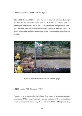
2.2.1.3 Vapour or liquid sensing tubes:
The leak detection technique by this method involves installation of these tubes all
over the pipelines. During the occurrence of the leak, the contents of the pipe gets in
contact with the tube. The concentration distribution is measured by forcing a
column of air into the tube with constant speed. Gas sensors are placed at the end of
each tube. The size of the leak is indicated by the peak in gas concentration caused
by every increase in gas concentration.

11
Figure 4: Liquid sensing technique, source Comini’s journal [12]
Figure 4 defines the technique of liquid sensing tubes. The electrolytic cell placed at
the detecting line constantly diffuses test gas into the tube. When the test gas passes
through the detector an end peak is produced which indicates the whole length of the
sensor tube [12]. Localization of the leak is nothing but the inverse ratio of leak peak
arrival to end peak arrival,
Although the method is very simple and appropriate for underground pipelines,
applying it to huge network is cost effective. Moreover, speed of detection of leak is
very low.
2.2.1.4 Liquid Sensing Cables.
In these cables energy pulses are sent out constantly throughout the length. As the
energy pulses travels, the reflected energy are stored in memory. The electrical
properties will be altered by the presence of liquids in the sensor which will wet the

12
cable if sufficiently present [13]. The alteration is used to determine the leak. This
method works well for short pipelines.
2.2.1.5 Soil Monitoring:
This method uses a tracer inside the pipeline [14]. Tracers are nothing but
inexpensive non-hazardous gas. The tracer is featured as a volatile gas which get
released at the exact location of the leak. By monitoring the soil above the pipeline,
the presence of leak can be localised. By this method, false alarm is very low and
small leaks can be detected easily. However, the method is expensive as tracer has to
be injected in the pipe which is not possible for uncovered pipelines.
Hardware based methods like acoustic, optical, cable sensor etc are less reliable
because they are noise sensitive
2.2.2 Software Based Systems
The project uses software techniques. The pipeline parameters like pressure, flow
and temperature are closely monitored. Some of these techniques are discussed
below.
2.2.2.1 Mass- Volume balance
This method has the principle of conservation of mass. Leak is determined by the
difference between the upstream and downstream flow [15]. This method is widely
used in oil pipelines The main drawback is that by this method the actual position of
the leak is unknown., hence, other methods are applied after the mass balance
method to localise the leak position soon after the leak is detected [19].

13
2.2.2.2 Real time transient modelling
This method of leak detection uses pipe flow models which are constructed by using
equations of conservation of mass, momentum and energy. The difference between
the measured and the estimated value is used to determine the leak. Billman and
Isermann[16] ,used this approach for leak detection and localization. In the study for
single leak, an algorithm for determining the leak location and finite estimation of
leak flow is developed. This method is very efficient because it can not only detect
the position of the leak accurately but also locate leaks as small as 1 percent of flow
[17]. However, the method is cost effective as it deals with huge data processing in
real.
2.2.2.3 Negative pressure wave
This method locates the leak by finding out the time difference taken by the negative
waves to arrive at the pressure sensors installed at the start and end of the pipeline.
These negative waves are nothing but pressure waves that are generated due to leaks
which cause sudden pressure drops which propagates with certain speed towards
both downstream and upstream in the pipeline. According to H. Chen, H. Ye. L.
Chen and H. Su [18] study, support vector machine learning is used to analyse the
pressure sensor data and locate the location of the leak. A nonlinear classifier is
trained using supervised learning to automatically detect the presence of leak in the
pressure curve. This study would locate small and slow leak out of noise. The
negative pressure wave along with signal processing technique is studies by Li yo bi.
By this method, the reported time delay is 2 minutes and the estimated error is 2%.
2.2.2.4 Pressure point analysis method
This method is based on the fact that pressure drops because of leak. It detects leak
by comparing the on running statistical trend and the current pressure value. By the
statistical analysis, the mean value of the pressure measurement of the new data and
the old data is compared. If the mean of the old data is larger than the mean of the

14
current data, the leak alarm is triggered [20]. This method is installation inexpensive
and can accurately identify the occurrence of leak. However false alarm is triggered
at times because pressure drop is not unique to leak occurrence.
2.2.2.5 Statistical Method
This method is implemented to reduce the rate of false alarm. This method is suitable
for oil pipeline systems. It uses advance statistical analysis to study the flow rate,
temperature and pressure values of a pipeline [21]. This method continuously
monitors for changes in the pipeline and relocation of pressure /flow instruments,
hence this method is an approximation for complex networks of pipeline. Detection
of 0.5% leaks was reported by Zhang and Mauro ‘s study [22].
2.2.26 Digital signal processing
The method compares the response to a known input over a period of time with the
measurements taken at later time and based on their wavelet transform or coefficient
frequency response, leak alarm is triggered [23]. The disadvantage of this method is
that, leak cannot be detected unless the size of the leak is not considerably large.
Hardware based leak detection methods are cost effective in terms of installation and
maintenance like service and repair. On the other hand, software based techniques
deal with implementation of algorithms to continuously monitor flow rate,
temperature and pressure of other pipeline parameters based on future study.
Software method is more popular because it is cost efficient.
The most common softwares used are COMSOL and Open foam. COMSOL is widely
used and encouraged because it works on the principle of finite element method.

15
2.3 Computational Fluid dynamics
CFD is a branch of fluid mechanics that solves fluid flow problems by using
algorithm based techniques. Turbulent or transonic flow requires high speed
computers that provide better solutions. The interaction between the liquids /gases
with surfaces defined by boundary conditions is performed by high speed computers
that simulate this interaction between them [24]. The Navier –Stokes equation is the
fundamental of all CFD problems.
ꝭ (
𝒅𝒖
𝒅𝒕
+ 𝒖. 𝛁𝒖)= -𝛁p+ F
The above equation holds true for incompressible Newtonian Fluid whose Mac
number is less than 0.3
p is the fluid pressure,
ꝭ is the fluid density, and
u is the fluid velocity and f is the sum of the inertial forces pressure forces and
viscous forces [25].
The finite element method (FEM) is a numerical method for finding approximate
solutions to boundary value problems for partial differential equations. The domain
of the problem is divided into a collection of sub domains, each sub domain
represented by a set of equations. Finally, these set of element equations are
recombined into a global system of equations for the final calculations [24].
The COMSOL software was introduced in 1986 that uses Finite element analysis
method, solver and Software packages for engineering and mathematical problems.
The partial differential equations are directly fed into the coupled systems to solve
problems related to different modules. Amongst the different modules available in
COMSOL, the pipe flow for both steady state and transient study of the town gas
mixture [26] is focussed as it satisfies the conditions of the type of fluid to be
analysed in this project.

16
Pipe Flow Module
The module is used in pipe systems in the oil and gas industry and chemical
processes. It is used for simulating flow in incompressible fluids in pipes and also
compressible hydraulic transients. The simulations provide velocity, temperature and
pressure variations in pipes. The physics uses the conservation of energy, momentum
and mass [26].
The pressure, flow and concentration across the cross sections of the pipe are
modelled as cross section averaged quantities varying along the length of the pipe
lines. The friction factors describe the pressure losses that occur along the length of
the pipe by the friction factor expressions. There is frictional pressure loss along the
pipe due to momentum change because of T joints, bends and valves. A broad range
of Darcy Friction factors cover the entire range from non-Newtonian and Newtonians
fluids, turbulent to laminar flow, geometries of different cross section and surfaces
with range of relative roughness values [26].
The module has 7 physics amongst which the following are of utmost utility.
Pipe Flow: It simulates velocity and pressure fields in isothermal pipelines.
Heat Transfer in Pipes: It computes the mass balance equation including the wall
heat transfer to the surroundings
Transport of Diluted Species in Pipes: It simulates the mass balance equation in
order to compute the dispersion, diffusion and convection of the solute in terms of
the concentration distribution.

17
Chapter 3
Initial calculation and experiments for Data Collection
3.1 Calculation of dynamic viscosity and density of the gas mixture
The dynamic viscosity and the density of the gas mixture is evaluated by the
composition details provided by of the town gas data sheet handed over by the
Singapore Power Limited [1] is as follows
Components Low Range High Range
Hydrogen 41 65
Methane 4 33
Ethane 0 2.6
Propane 0 1.3
Butane 0 1.7
Pentane 0 5
Carbon Monoxide 2 6
Carbon Dioxide 9 20
Nitrogen 2 10
Oxygen 0.5 2.5
Assumption: The dynamic viscosity of the gas mixture is found out by considering
the low range of the components of the gas mixture. Below formula is used for
calculating the dynamic viscosity
µga=
∑ 𝑦𝑖µ𝑖√𝑀𝑔𝑖𝑁
𝑖=1
∑ 𝑦𝑖√𝑀𝑔𝑖𝑁
𝑖=1
where
µga= Dynamic viscosity of gas mixture.
yi = Mole fraction of the ith component of the gas mixture.
µi = Dynamic viscosity of ith component of the gas mixture.
Mgi = Molecular weight of ith component of the gas mixture[27].

18
Calculated density and dynamic viscosity of the gas mixture
Gas Dynamic Viscosity
(Pa-s)
Mole Fraction
(No Unit)
Hydrogen 8.85x10-6
0.7008
Methane 2x10-5
0.0684
Carbon Monoxide 1.77x10-5
0.03
Carbon dioxide 1.50x10-5
0.1538
Nitrogen 1.77x10-5
0.0342
Oxygen 2.05x10-5
0.0085
Table 1: Density and dynamic viscosity of the components of the gas mixture
By using the above equation, the Dynamic Viscosity of the gas mixture is calculated
to be 1.367x10^(-5) Pa –s
To calculate the Specific gravity of the mixture
Specific gravity= ρ/ρ_air
ρ - density of gas mixture = 1.205 kg/m3
ρ_air - density of air=0.6025 kg/m3
Therefore, Specific Gravity of gas mixture=0.5
The density and dynamic viscosity values are used for network simulation in
COMSOL.
3.2 The Test Bed Setup
The test bed has 4 pipeline connected in the form of a rectangle. The length of the
rectangle is 10 m and breadth is 1 m. The joints connecting the two pipelines are
made up of ductile iron. The outer diameter of the pipeline is 150 mm with a width
of 10 mm. A couple of flow meters and pressure meters are installed on the network.
A data logger is used to study the signals generated by these sensors.

19
3.2.1 Pressure meter: ABB Model 266GSH gauge
It has a LCD display of 128*64 pixels. The turn on time with minimum damping is
less than 10s. The transmitter works from 10.5 V to 42V DC with no load. The
output signal is two wires 4 mA to 20mA. The transmitter is configured with HART
and Foundation Field bus communication as per customers’ specified range. The
signals to be studied need fast response time so Hart Communication is configured in
this case.
Figure 5: Pressure meter ABB Model 266GSH gauge
3.2.2 Flow meter: ABB PitoMaster FPD550
Pitometer is an averaging pitot -tube based flow meter. It is advantageous over
convectional DP flow meters because it avoids the problems involved in installation,
selection, sizing and commissioning. It is wide screen LCD; 128*64 pixel display.

20
Fluids that are supported are saturated steam, gases and liquids. Output Signal is 4
mA to 20 mA, selected for square root output. Hart Communication is configured.
Figure 6: Flowmeter ABB PitoMaster FPD550
3.2.3 Data Logger: ABB Screen Master RVG200; Paperless recorder
The data in the logger is highly encrypted with storage complaint to 21 CFR. It has
internal memory of 2 GB. It has 2 USB ports. Power supply required is 100V to 240
V, 20/60 Hz. It has number of communication configuration options like Ethernet,
FTP, Email, MODBUS TCP and RS485 communication

21
Figure 7: Data Logger: ABB Screen Master RVG200
The figure 8 shows the test bed arrangement
Figure 8: The test bed setup

22
3.3 Studying pressure profile of the leak.
In the gas pipeline network, the gas flowing in the pipeline is of low pressure. When
a leak occurs the following observations are made
1. There is a peak occurring at the leak point having the highest pressure
difference
2. The leak point near the source shows a higher peak and the peak decreases as
the leak point move away from the source.
The pressure difference evaluated is the difference between the atmospheric pressure
and the no leak pressure for a given point. The pressure profile for a network
constructed on COMSOL and simulated for no leak is as shown in figure 9.
Figure 9: Pressure profile for no leak condition

23
The source is considered to be at point (0,0)
The leak points are considered at the coordinates (0,-0.5),(0.5,-1),(1,-1.5),(1.5,-2).
Figure 10: Pressure profile for different leak points
 When the leak is at point 1 i.e (0,-0.5) ,the shoot of the peak is highest at the
same point indicating it to the leak point which is true in this case.
 When the leak is at point 2 i,e (0.5,-1) , the shoot of the peak for this point is
comparatively less because it is more away from the source than the point 1.
However, the peak is at point 2 indicating it to be the leak point. Hence it
accurately identifies it.
 When the leak is at point 3 i.e (1, -1.5), the shoot of the peak further reduces
as it more away from the source compared to the point1 and point 2. However
the peak at point 3 indicates it to be leak point which is correctly detected.
Hence the experiment supports the theory stated.

24
3.4 Data organization
3.4.1. The similar network as the test bed is used to generate data
.
..
Figure 11: The network setup
There are 4 pipelines namely CD and AB 10 m each and AC and BD are 1 m each.
216 leak positions (99 points on each CD and AB and 9 points each on AC and BD)
are considered all over the network and 2200 positions (1000 points each on CD and
AB and 100 points each on AC and BD) of pressure are measured for stationary
study with inlet of 0.4 m^3 /s volumetric flow and outlet pressure of 1.01*10^5 Pa.
Positive x is along CD and positive y is along CA.
Below is the pressure profile of the network without leak.
1m
m
m
M
0
Inlet Outlet
C
D
BA
a
10 m

25
Figure 12: Pressure profile of the network on no leak condition
Below is the pressure profile when leak is induced in the network to study the effect
in parametric sweep.
Figure 13: Pressure profile of the network on leak condition

26
The network simulated is run in COMSOL by the parametric sweep for 216
parameters for 2200 points all over the designed frame of network for stationary
study. The data is collected in matrix of 2200*216 for pipes AB and CD and 2200*9
for AC and BD.
All these data are collected in xml file and using MATLAB these files are converted
to csv files. A sample of the data is shown below.
x y z 0.1 0.2 0.3 0.4 0.5
p (Pa) p (Pa) p (Pa) p (Pa) p (Pa)
0 0 0 102499.131 102515.687 102531.771 101582.787 102562.554
0.01 0 0 101499.414 101526.875 101553.74 101580.018 101605.72
0.02 0 0 101496.554 101524.046 101550.941 101577.25 101602.981
0.03 0 0 101493.694 101521.217 101548.143 101574.482 101600.243
0.04 0 0 101490.834 101518.388 101545.344 101571.713 101597.504
0.05 0 0 101487.975 101515.559 101542.546 101568.945 101594.765
0.06 0 0 101485.115 101512.73 101539.747 101566.176 101592.027
0.07 0 0 101482.255 101509.901 101536.949 101563.408 101589.288
0.08 0 0 101479.395 101507.072 101534.15 101560.639 101586.549
0.09 0 0 101476.535 101504.243 101531.351 101557.871 101583.811
0.1 0 0 101473.675 101501.414 101528.553 101555.103 101581.072
0.11 0 0 101474.789 101498.585 101525.754 101552.334 101578.334
0.12 0 0 101475.902 101495.756 101522.956 101549.566 101575.595
0.13 0 0 101477.016 101492.927 101520.157 101546.797 101572.856
0.14 0 0 101478.129 101490.098 101517.359 101544.029 101570.118
0.15 0 0 101479.242 101487.269 101514.56 101541.26 101567.379
0.16 0 0 101480.356 101484.439 101511.761 101538.492 101564.64
0.17 0 0 101481.469 101481.61 101508.963 101535.723 101561.902
0.18 0 0 101482.583 101478.781 101506.164 101532.955 101559.163
0.19 0 0 101483.696 101475.952 101503.366 101530.187 101556.424
0.2 0 0 101484.81 101473.123 101500.567 101527.418 101553.686
0.21 0 0 101485.923 101474.245 101497.768 101524.65 101550.947
0.22 0 0 101487.037 101475.367 101494.97 101521.881 101548.209
0.23 0 0 101488.15 101476.49 101492.171 101519.113 101545.47
0.24 0 0 101489.264 101477.612 101489.373 101516.344 101542.731
0.25 0 0 101490.377 101478.734 101486.574 101513.576 101539.993
Table 2: Sample data set

27
At different coordinates of x, y and z, pressure values for leak points by parametric
sweep is collected. By parametric study, the parameter values can be changed by a
range specified. Here the range varies from 0 to 216 leak points. The collected data is
then used for simulations in MATLAB.
3.5 Data Analysing Methods
In the following, we describe the different methods of data analysis.
3.5. 1 Data Mining:
It is a method of analyse huge data and then convert them into useful facts and
information. It refers to the method of extracting facts from knowledge stores
3.5.2Data Mining Tasks
The following are the tasks for data mining. The methods of analysis depend upon
the kind of task that is needed to be done. Different methods of data mining include
linear regression, support vector machine, classification and Regression Tree and
artificial neural network.
3.5.3 Description and Summarization
Each data analysis in the beginning needs to look for quick general trends and
supreme values. Getting familiar with the data, to obtain a concept of what the data
might be able to contain, is important. More analyzing steps might have to be done
for the data to be suitable. Purpose of analysis towards definite features, data quality
difficulties and additionally required background facts will be at one's control if he
gets the concept of overview. Tools like summary tables, simple descriptive statistics
and simple graphics are necessary prerequisite to get this task done.

28
3.5.4 Descriptive Modelling
We use descriptive modelling to find out the particular model for the data.
Smoothing, density estimation, clustering and data segmentation are the different
steps of descriptive modelling. K means clustering is the most widely used clustering
method. Cluster analysis is the method in which data set that contains natural clusters
which when discovered is characterized and labelled.
3.5.5 Predictive Modelling
To predict the characters of new events and get more information, many models are
usually built. The aim is to construct a model that will allow the value of one variable
to be predicted from the familiar values of different variables. Predictive modelling is
categorized in the group of supervised learning hence one variable is labelled as
target variable and will be described as a function of different variables. Type of
model is determined by the nature of the target variables.
3.5.6 Discovering Patterns and Rules
Sometimes it becomes difficult to achieve functional relationships in a meaningful
way. In that context, Association Rules originated from market basket analysis.
Pattern behaviour methods like Association Rules are used.
3.5.7 Retrieving Similar Objects:
Search engine based keywords and indexed meta information is used to quickly find
the desired similar objects .This method works good for text as well as image data.

29
Chapter 4
Results
In this chapter, first the different techniques are discussed, followed by an intensive
analysis of the effects of the methods on the detection of the leak for single inlet and
multiple inlet values. Among the methods mean square error and k nearest
neighbour are studied. For multiple inlet values multidimensional scaling method is
used to identify the pipes having leak accurately.
4.1 Approaches of analysis for single inlet value
The aim of the experiments is to predict the leak location even in the presence of
noise. The noise considered is the randomly added noise (Gaussian Noise). Gaussian
noise is any recognized amount of unexplained variation whose normal distribution
function is equal to probability distribution function. The mean absolute error (MAE)
is value used to find out how close forecasts or predictions of the leak points are to
the true locations of the leak. Leave one leak position out (LOO) method is used for
different methods of study. In LOO technique, for each leak position, the trace
position data is removed from whole of the data set, and then noise is added to the
test point and mean absolute error is computed.
4.1.1 Mean Square difference Approach
The square difference between the actual pressure and the randomly added noise
pressure for each leak position for every 2200 points on the network is calculated.
The minimum square difference is found out .The index of this minimum value is the
predicted location of the leak
The following steps have been taken to calculate the mean square error

30
Start
Generate pressure for
each leak point
Choose ‘i’th leak point
and add noise
Compute MSE for
‘i’th vector with
noise and actual data
Is the MSE
for the
position
minimum?Compute
accuracy
Plot MAE vs
noise%
yes no
Stop

31
The accuracy of detection against the randomly added Gaussian noise is shown in the
figure 14
Accuracy of detection is 12% when the Gaussian noise level is 0 %.
Accuracy of detection is 0 % when the Gaussian noise level is 100%
The noise is added at the interval of 5, over 20 points for the Gaussian noise. By the
100% addition of Gaussian noise, the maximum absolute error that can be incurred is
of 0.36 metre.
Figure 14: Accuracy vs Gaussian noise

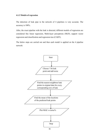
32
The standard deviation is calculated at an interval of 5 over 20 points by adding
hundred Gaussian noise and output is showed as in figure 15.
Figure 15: Error bar for mean square method
4.1.2 Knn Approach
K nearest neighbour is a simple algorithm that classifies different cases based on
distance function. Distance can be Euclidean, Manhattan or Minkowski distance. A
case is classified by the majority votes given by the neighbours with the case being
assigned to the class which is most common among its k nearest neighbours.
Following are the steps that are taken to calculate MAE using knn method.
Gaussian noise level [%]
Meanabsoluteerror[m]

33
At every interval of 5,one hundred different Gaussian noise is added to find out the
standard deviation and the table 1 shows the values of the MSE for k=1 , 2, 3,4 and
5 for different noise levels. The figure 16 shows the standard deviation
corresponding to the noise level.
Start
Choose ‘i’th leak point and
add noise
Find the nearest neighbour leak points in
original data for every corresponding row of
leak points added with noise
Find the mean of the locations
of the predicted leak points
points
Plot MAE vs noise%
and error bar
Stop
Stop

34
Table 3: MSE values for k=1 to k=5 for Gaussian noise levels
Figure 16: Error bar for Knn Method
Gaussian Noise level [%]
Meanabsoluteerror[m]

35
4.1.3 Models of regression
The detection of leak pipe in the network of 4 pipelines is very accurate. The
accuracy is 100%.
After, the exact pipeline with the leak is detected, different models of regression are
considered like linear regression, Multi-layer perceptrons (MLP), support vector
regression and classification and regression tree (CART).
The below steps are carried out and then each model is applied on the 4 pipeline
network
Start
Choose ‘i’th leak
point and add noise
Find the nearest neighbour leak
points in original data for every
corresponding row of leak
points added with noise
Find the mean of the locations
of the predicted leak points
points
Plot MAE vs noise%
Stop

36
4.1.3.1 Linear Regression
It is an approach of modelling the relationship between dependent variable and
independent variable. The independent variable is pressure and the dependent
variable is the coordinates of the leak location (x and y coordinate).Linear regression
is commonly fitted using least square method. The benefit of this method is , it is
used for prediction and error reduction by fitting a prediction model using observed
data.
4.1.3.2 MLP
A multilayer perception (MLP) is a feed forward artificial neural network that
models the appropriate outputs by mapping them to the input data. MLP consists of
layers of nodes called neurons in the form of a directed graph with one layer
connected to the next layer in consequence. The back propagation technique is used
for training the network. The main application of MLP is in pattern recognition and
supervised learning.
4.1.3.3 Support Vector Machine
Support Vector machine can either be used as classification method or regression
method both of which are supervised learning techniques. In case of classification,
the output is a real number hence prediction becomes difficult because it can take up
infinite values. An upper and lower limit known as epsilon is set in as per the
requirement of the problem. There are two types of SVM classification, linear and
non linear .In linear SVM, the trained dataset of n points of 2 groups is divided by
maximum margin hyperplane. The plane is defined order to maximise the distance
between the nearest point from either group and the hyperplane. A nonlinear
classifier is based on the kernel to maximum–margin hyperplane. The algorithm fits
the maximum- margin hyperplane into a transformed feature space. Feature space

37
consists of feature vectors which are nothing but numerical featured n dimensional
vectors that define some specific object. The transformation may be done non-
linearly. In SVM regression, input is mapped onto m dimensional feature space by
using fixed nonlinear mapping and then linear model is constructed in the feature
space. A upper and lower limit known as epsilon is set in as per the requirement of
the problem. However the main idea remains the same; to minimize error.
4.1.3.4 CART
A decision tree learning method utilizes decision trees as predictive models. Models
where target variables take up some definite value set it is called classification tree.
Decision trees where the target variables take up continuous values is called
regression tree. This method is more liable to over fitting of the curve.
4.2 Approaches of analysis for multiple inlet values
After considering only one inlet value and carrying out above analysis, focus shifts to
notice the effect of multiple inlet value. A simple case of 5 inlet values and a total of
twelve leak locations, three equidistant leak locations in each pipe is considered
.
..
Figure 17: The network with leak locations drawn in circles.
1m
m
m
M
0
Inlet Outlet
C
D
BA
a
10m

38
There are 4 pipelines namely CD and AB 10 m each and AC and BD are 1 m each.
12 leak positions(3 equidistant leak points on each CD , AB, AC and BD) are
considered all over the network and 2200 positions (1000 points each on CD and
AB and 100 points each on AC and BD) of pressure are measured for stationary
study with 5 different inlet values of 0.5 m^3 /s , 0.6 m3
/s, 0.7 m3
/s, 0.8m3
/s, 0.9
m3
/s volumetric flow and outlet pressure of 1.01*105
Pa.
The Multi dimensional scaling and Principle component analysis is run in MATLAB
to show cluster as in figure 17.
Red circles - pipeline CD
Blue circles – pipeline AB
Green circles – pipeline AC
Black circles – pipeline BD
Multidimensional scaling (MDS) is a method by which levels of similarity between
individual cases of a set of data can be visualized. The good separation between these
four pipelines helps to conclude that the pipe having leak is accurately predicted.

39
Figure 18: MDS graph for the network showing the separation between the pipelines.

40
Chapter 5
Conclusion and future work
5.1 Conclusion
The detection of leak is a very critical problem for the whole underground gas
network in Singapore. Currently implemented methods are cost and labour intensive.
To ensure reliability, real time monitoring of the network is demanded and hence the
project comes into the picture [28].
The conclusion can be drawn from the results as seen in section 3.3 in chapter 3 and
chapter 4. In this thesis, it is verified how the leak location is affected by the position
of the inlet source. It is also found out how the pressure at a point varies when there
is a leak condition and no leak condition which would help to build predictive
maintenance models, so that it could avoid leaks to facilitate better localisation
system. It is observed that nearer the leak to the source inlet better is its detection.
It is also clearly observed that the effect of the noise tend to decrease the accuracy of
detection of leak in the pipelines. Also the different methods of analysis like mean
square and k nearest neighbour is studied and how the Gaussian noise affect the
mean absolute error is depicted through graphs. The standard deviation on addition
of hundred random Gaussian noises can be clearly observed through the graphs.
More the noise more is the deviation and hence more is the mean absolute error.
It has also been clearly shown that the leak pipe can be located accurately by the
good spacing between the pipelines shown by the multi dimensional spacing graph
for multiple inlet values.
By performing different analysis, it can be clearly demonstrated how the noise
percentage impacts the detection of leak. Hence the observation can be incorporated
in the advance predictive models in order to avoid leakages in pipeline networks.

41
5.2 Future Work
Though the objective is fulfilled, the major limitation of the thesis was the data,
which was generated from COMSOL as real life data was not available. Although
the network simulated was identical to the actual test bed, real life data should be
taken for more detailed and accurate results.
A large number of points are considered all around the four pipe network assuming
all the points to have pressure sensors which may not be the actual scenario. The
sensors should be placed at optimised locations to detect leak in the whole network.
Minimum sensors should be used to have a cost effective system.
In this thesis focus was on mean square method and k nearest neighbour method.
There are a number of ways and techniques that can be added to this analysis and a
comparative study can be done. The work can be extended further by extending the
network and considering multiple inlets and outlets at the same time instance.
Also, since the data generated is huge the compilation and computing time is too
long. For this reason, some variable optimization procedures can also be applied to
reduce the computation time.
Further, a simple quantitative analysis and testing of data are not enough to build a
predictive model for the pipeline networks. Using the physical parameters, RFID
traceability information and data generated, advanced data analytics can be
performed for location identification. Practical testing of several parameters is
needed to be done to validate the research findings as whole of the pipeline network
is underground. Analytics could be extended to predictive maintenance to identify
future failure -prone zones.

42
Appendix
1.Reference code for mean square method
close all;
clear all;
clc;
res_1 = [];
res_2 = [];
xx=100*[0:0.05:1];
%the same with LOO without and with noise
for i=1:21
noise_level = i*0.05-0.05;
clear aa bb;
for j=1:100
[aa,bb]=skrypt_LOO_std(noise_level, j);
%with noise
res_2(i,j) = mean(abs(bb(:,3)-bb(:,4))); %mean absolute error of the leak location
end
end
res_3(:,1) = mean(res_2');
res_3(:,2) = std(res_2');
figure(1);
errorbar(xx,res_3(:,1),res_3(:,2),'LineWidth',1.5);
function [odp_1, odp_2] = skrypt_LOO(noise_level,r_seed);
%close all;
%clear all;
%clc;
%noise_level = 0.05;
rng(r_seed);
load pipedata;
clear p p_err loc locloc;
p=[p1,p2,p3,p4];
loc=[loc1,loc2,loc3,loc4];
locloc(1:99)=1;
locloc(100:198)=2;
locloc(199:207)=3;
locloc(208:216)=4;
p_err = zeros(216,216);

43
%%for clean data
for i=1:216
for j=1:216
p_err(i,j)=sum((p(:,i)-p(:,j)).^2)/2200;
if(i==j)
p_err(i,j)=inf;
end
end
end
clear tmp1 tmp2;
for i=1:216
[tmp1(i),tmp2(i)]=min(p_err(i,:));
end
clear odp_1;
tmp_acc = [1:216];
odp_1 = [tmp_acc',tmp2',loc(tmp2)',loc',locloc(tmp2)',locloc'];
%%for data with noise
clear p_noise;
for i=1:216
clear tmp_noise;
tmp_noise = noise_level*(max(p(:,i))-min(p(:,i)))*randn(2200,1);
p_noise(:,i)=p(:,i)+tmp_noise;
end
clear p_noise_err;
for i=1:216
for j=1:216
p_noise_err(i,j)=sum((p_noise(:,i)-p(:,j)).^2)/2200;
if(i==j)
p_noise_err(i,j)=inf;
end
end
end
clear tmp1_noise tmp2_noise;
for i=1:216
[tmp1_noise(i),tmp2_noise(i)]=min(p_noise_err(i,:));
end
clear tmp_acc_noise acc_2 odp_2;
tmp_acc_noise = [1:216];
odp_2 = [tmp_acc_noise',tmp2_noise',loc(tmp2_noise)',loc',locloc(tmp2_noise)',locloc'];
2. Reference code for knn method
close all;
clear all;
clc;
res_21 = [];
res_22 = [];
res_23 = [];
res_24 = [];

44
res_25 = [];
xx=100*[0:0.05:1];
K_max = 5;
%for j=1:K_max %K parameter
for i=1:21
clear a;
for h=1:100
clear a;
a=skrypt_LOO_knn_std(noise_level,1,h);
res_21(i,h) = mean(abs(a(:,1)-a(:,2)));
clear a;
res_22(i,h) = mean(abs(a(:,1)-a(:,2)));
clear a;
res_23(i,h) = mean(abs(a(:,1)-a(:,2)));
clear a;
res_24(i,h) = mean(abs(a(:,1)-a(:,2)));
clear a;
res_25(i,h) = mean(abs(a(:,1)-a(:,2)));
end
end
%end
%%%%%%%%%%%%%%%%%%%
res_31(:,1) = mean(res_21');
res_31(:,2) = std(res_21');
res_32(:,1) = mean(res_22');
res_32(:,2) = std(res_22');
res_33(:,1) = mean(res_23');
res_33(:,2) = std(res_23');
res_34(:,1) = mean(res_24');
res_34(:,2) = std(res_24');
res_35(:,1) = mean(res_25');
res_35(:,2) = std(res_25');
color_list = ['r' 'g' 'b' 'k' 'm' 'c' 'y'];
figure(1);
hold on;
clear legend_txt;
legend_txt = {};
errorbar(xx,res_31(:,1),res_31(:,2),'LineWidth',1.5,'Color',color_list(1));
legend_txt{1} = strcat('K=',num2str(1));

45
box on;
xlabel('Gaussian noise level [%]');
ylabel('Mean absolute error [m]');
legend(legend_txt,'Location','NorthWest');
%Table_2: WITH_LOO; first column - noise_level, then MAE for K=1...K_max
[xx',mean(res_21')',mean(res_22')',mean(res_23')',mean(res_24')',mean(res_25')']
unction [loc_err] = skrypt_LOO_knn_std(noise_level,K,r_seed);
%close all;
%clear all;
%clc;
rng(r_seed);
load pipedata;
clear p p_err loc locloc loc_err pred_loc;
p=[p1,p2,p3,p4];
locloc(1:99)=1;
locloc(100:198)=2;
locloc(199:207)=3;
locloc(208:216)=4;
clear p_noise;
for i=1:216
clear tmp_noise;
end
for i=1:216
clear idx_knn idx_data loc_tmp;
idx_data = [1:216];
idx_data = idx_data(find(idx_data~=i));
loc_tmp = loc(idx_data);
idx_knn=knnsearch(p(:,idx_data)',p_noise(:,i)','K',K);
pred_loc(i) = mean(loc_tmp(idx_knn));
end
loc_err = [loc',pred_loc'];
3. Reference Code for classification methods
close all;

46
clear all;
clc;
res_1 = [];
res_2 = [];
xx=100*[0:0.05:1];
%just after adding the noise; NO LOO!
%for i=1:21
% i
% noise_level = i*0.05-0.05;
% clear a;
% a=skrypt_classification(noise_level);
% res_1(i) = mean(abs(a(:,1)-a(:,2))); %mean absolute error of the leak location
%end
for i=1:21
i
for j=1:10
clear a;
a=skrypt_LOO_classification_std(noise_level,j);
res_2(i,j) = mean(abs(a(:,1)-a(:,2)));
end
end
res_3(:,1) = mean(res_2');
res_3(:,2) = std(res_2');
color_list = ['r' 'g' 'b' 'k' 'm' 'c' 'y'];
figure(1);
hold on;
clear legend_txt;
legend_txt = {};
box on;
xlabel('Gaussian noise level [%]');
ylabel('Mean absolute error [m]');
%noise_level, MAE
[xx',mean(res_2')']
function [loc_err] = skrypt_LOO_classification_std(noise_level,r_seed);
%close all;
%clear all;
%clc;
rng(r_seed);

47
load pipedata;
clear p p_err loc locloc loc_err pred_loc;
p=[p1,p2,p3,p4];
locloc(1:99)=1;
locloc(100:198)=2;
locloc(199:207)=3;
locloc(208:216)=4;
% STANDARDIZATION
p=zscore(p);
clear p_noise;
for i=1:216
clear tmp_noise;
end
for i=1:216
clear m1 m2 m3 m4 idx_data locloc_tmp;
idx_data = [1:216];
idx_data = idx_data(find(idx_data~=i));
loc_tmp = loc(idx_data);
locloc_tmp = locloc(idx_data);
p_tmp=p(:,idx_data);
clear c1 c2 c3 c4;
c1=find(locloc_tmp==1);
%NEURAL NETWORKS
%m1=feedforwardnet(10); %number of neural neurons in hidden layer
%m1.trainParam.showWindow = 0;
%m1 = train(m1,p_tmp(:,c1),loc_tmp(c1));
%m2=feedforwardnet(10);
%NONLINEAR REGRESSION
%m1=fitnlm(p_tmp(:,c1)',loc_tmp(c1)');
%LINEAR REGRESSION
%m1=fitlm(p_tmp(:,c1)',loc_tmp(c1)','quadratic');

48
%LINEAR REGRESSION
m1=fitlm(p_tmp(:,c1)',loc_tmp(c1)');
%SVR
%m1=svmtrain(loc_tmp(c1)',p_tmp(:,c1)','-s 3');
%CART
%m1=fitrtree(p_tmp(:,c1)',loc_tmp(c1));
if(locloc(i)==1)
%SVR
%pred_loc(i)=svmpredict(loc(i),p_noise(:,i)',m1);
pred_loc(i)=predict(m1,p_noise(:,i)');
%NEURAL NETWORKS
%pred_loc(i)=net(m1,p_noise(:,i));
end
if(locloc(i)==2)
%SVR
%NEURAL NETWORKS
end
if(locloc(i)==3)
%SVR
%NEURAL NETWORKS
end
if(locloc(i)==4)
%SVR
%NEURAL NETWORKS
end
end
loc_err = [loc',pred_loc'];
4. Reference code for multiple input values close all;
clear all;
clc;
p = [];
clear d;
d=xlsread('data_inlets (#MAHATO LIPIKA#).xlsx',1);
p1_1 = d(2:end,4:6);
clear d;

49
p1_2 = d(2:end,4:6);
clear d;
p1_3 = d(2:end,4:6);
clear d;
p1_4 = d(2:end,4:6);
clear d;
p1_5 = d(2:end,4:6);
clear d;
p2_1 = d(2:end,4:6);
clear d;
p2_2 = d(2:end,4:6);
clear d;
p2_3 = d(2:end,4:6);
clear d;
p2_4 = d(2:end,4:6);
clear d;
p2_5 = d(2:end,4:6);
clear d;
p3_1 = d(2:end,4:6);
clear d;
p3_2 = d(2:end,4:6);
clear d;
p3_3 = d(2:end,4:6);
clear d;
p3_4 = d(2:end,4:6);
clear d;
p3_5 = d(2:end,4:6);
clear d;
p4_1 = d(2:end,4:6);
clear d;
p4_2 = d(2:end,4:6);
clear d;
p4_3 = d(2:end,4:6);
clear d;
p4_4 = d(2:end,4:6);
clear d;

50
p4_5 = d(2:end,4:6);
%pressure; pipe; inlet; location
p = [p;p1_1(:,1),repmat(1,size(p1_1,1),1),repmat(1,size(p1_1,1),1),repmat(1,size(p1_1,1),1)];

51
pp=[p1_1,p1_2,p1_3,p1_4,p1_5,p2_1,p2_2,p2_3,p2_4,p2_5,p3_1,p3_2,p3_3,p3_4,p3_5,p4_1,p4_2,p
4_3,p4_4,p4_5];
%pipe; location; inlet;
pp_2=[
1,1,1;1,2,1;1,3,1;
1,1,2;1,2,2;1,3,2;
1,1,3;1,2,3;1,3,3;
1,1,4;1,2,4;1,3,4;
1,1,5;1,2,5;1,3,5;
2,1,1;2,2,1;2,3,1;
2,1,2;2,2,2;2,3,2;
2,1,3;2,2,3;2,3,3;
2,1,4;2,2,4;2,3,4;
2,1,5;2,2,5;2,3,5;
3,1,1;3,2,1;3,3,1;
3,1,2;3,2,2;3,3,2;
3,1,3;3,2,3;3,3,3;
3,1,4;3,2,4;3,3,4;
3,1,5;3,2,5;3,3,5;
4,1,1;4,2,1;4,3,1;
4,1,2;4,2,2;4,3,2;
4,1,3;4,2,3;4,3,3;
4,1,4;4,2,4;4,3,4;
4,1,5;4,2,5;4,3,5;
];

52
References
[1] “City Gas “2009(May)
[2] www.powergas.com.sg
[3] www.brightminds.com.sg
[4] (Szoplik, The Gas Transportation in a Pipeline Network)
[5] (Payal & Kar, 2016)advanced multisensor anamolymonitoring and analytics for
gas pipeline
[6]Murvay, Pal Stefan A survey on gas leak detection and localization tecniques
2012
[7] Zhao Yang, Mingliang Liu, Min Shao, Yingie Ji Research on Leakage Detection
and Analysis of Leakage Point in the Gas Pipeline System September 15, 2011
[8] Furness, R. A., van Reet, J., 2009. Pipeline leak detection techniques. In: E.W.,
M. (Ed.), Pipeline Rules of Thumb Handbook. Elsevier, pp. 606–614.
[9] Brodetsky, I., Savic, M., 1993. Leak monitoring system for gas pipelines. In:
Acoustics, Speech, and Signal Processing, 1993. ICASSP-93., 1993 IEEE
International Conference on. Vol. 3. IEEE, pp. 17–20.
[10] Weil, G., 1993. Non contract, remote sensing of buried water pipeline leaks
using infrared thermography. ASCE, New York, NY(USA)., 404–407.
[11] Bennett, C., Carter, M., Fields, D., 1995. Hyperspectral imaging in the infrared
using liftirs. In: Proceedings of SPIE. Vol. 2552. p. 274.
[12] Comini, E., Faglia, G., Sberveglieri, G., 2009. Solid state gas sensing. Springer
Verlag.
[13] Sandberg, C., Holmes, J., McCoy, K., Koppitsch, H., sep/oct 1989. The
application of a continuous leak detection system topipelines and associated
equipment. Industry Applications, IEEE Transactions on 25 (5), 906–909.

53
[14] Lowry, W., Dunn, S., Walsh, R., Merewether, D., Rao, D., March 2000. Method
and system to locate leaks in subsurface containment structures using tracer gases.
US Patent 6,035,701
[15] Parry, B., Mactaggart, R., Toerper, C., 1992. Compensated volume balance leak
detection on a batched LPG pipeline. In:Proceedings of the International Conference
on Offshore Mechanics and Arctic Engineering. American Society of Mechanical
Engineers, pp. 501–501
[16] Billmann, L., Isermann, R., 1987. Leak detection methods for pipelines.
Automatica 23 (3), 381–385.
[17] Scott, S., Barrufet, M., 2003. Worldwide Assessment of Industry Leak Detection
Capabilities for Single & Multiphase Pipelines.Tech. rep., Dept. of Petroleum
Engineering, Texas A&M University.
[18] Chen, H., Ye, H., Chen, L., Su, H., 2004. Application of support vector machine
learning to leak detection and location inpipelines. In: Instrumentation and
Measurement Technology Conference, 2004. IMTC 04. Proceedings of the 21st
IEEE.Vol. 3. IEEE, pp. 2273–2277.
[19] Liu, A. E., February 2008. Overview: Pipeline Accounting and Leak Detection
by Mass Balance, Theory and Hardware Implementation.
[20] Farmer, E., et al., 1989. A new approach to pipe line leak detection. Pipe Line
Industry;(USA) 70 (6), 23–27.
[21] Zhang, X., 1993. Statistical leak detection in gas and liquid pipelines. Pipes &
pipelines international 38 (4), 26–29.
[22] Zhang, J., Di Mauro, E., 1998. Implementing a Reliable Leak Detection System
on a Crude Oil Pipeline. In: Advances inPipeline Technology, Dubai, UAE.
[23] Golby, J., Woodward, T., 1999. Find that leak [digital signal processing
approach]. IEE review 45 (5), 219–221
[24]Book J anderson , E Dick, Computational Fluid Dynamics, 3rd
Edison.

54
[25] Online What is Navier Stoke’s Equation
[26]Book Comsol Multipysics User Guide version 4.3
[27]Time-dependent mathematical modelling of binary gas mixture in facilitated
transport membranes (FTMs): A real condition for single-reaction mechanism.
[28] R. Sugunakar Reddy, Gupta Payal, Pugalenthi Karkulali, Mishra Himanshu
Leak detection in low pressure gas pipeline using pressure and flow variation

Master Thesis

Recommended

Recommended

More Related Content

Similar to Master Thesis

Similar to Master Thesis (20)

Master Thesis