SlideShare a Scribd company logo
1 of 76
Download to read offline
Macroeconometrics of Investment and the
User Cost of Capital ∗
Thethach Chuaprapaisilp
Fordham University
dom.thc@gmail.com
April 14, 2009
Abstract
The paper develops a general equilibrium macroeconometric model to estimate the
long-run user cost elasticity of business investment that is commonly discussed in the
macro investment literature. The user cost elasticity measures the responsiveness of
a representative firm’s desired level of capital stock (hence its investment in a given
period) to the change in its user cost of capital. The notion of the cost of capital being
used is that of Jorgenson (1963) where the user cost is the real rental price of capital
services or the after-tax costs of holding capital (interest/opportunity cost of finance
plus depreciation cost less capital gain) over a given period. The user cost elasticity is
also equivalent to the underlying elasticity of substitution between capital and labor
for the constant elasticity of substitution (CES) production function.
∗
I am grateful for the advice and guidance from my dissertation committee, my mentor Prof. Bartholomew
J. Moore and my readers Prof. Erick W. Rengifo and Prof. Hrishikesh D. Vinod. Special thanks to Prof. Hunt-
ley Schaller of Carleton University for providing Canadian cost of capital taxation data and to the Macroeco-
nomic and Quantitative Studies division at the Federal Reserve Board for the U.S. data. I also benefited from
comments and suggestions provided by participants from the Economics department during the Fordham
University Graduate Students session at the 2009 Eastern Economic Association conference.
1
Structural cointegrated vector autoregression (CVAR) methodologies, as described
in Garratt et al. (2006) and Juselius (2006), are employed based on a set of theoretically
consistent long-run relationships among macroeconomic variables. A small system of
log-linearized equations that represents a general equilibrium economy with investment
over the long run is derived and estimated. The model is further extended to incorpo-
rate a technological trend in production and investment associated with research and
development capital.
The estimation results provide evidence that the user cost capital is endogenous
to the general equilibrium system and responses to macroeconomic shocks including
external and policy shocks. Net exports are also endogenous to the firm’s investment
decision and can produce an upward bias to the estimated user cost elasticity of around
one percentage point due to equilibrium current account adjustments when compared
with the benchmark user cost elasticity of around -0.7 to -1.1. The endogeneity of
the user cost of capital that is influenced by domestic supply and demand for capital
in a large open economy also produces a smaller user cost elasticity by around half a
percentage point. Thus the study addresses the issue of wide-ranging user cost elasticity
estimates obtained in the literature and provides some guidance for future research.
1 Introduction
The cost of capital is considered an important factor affecting firms’ investment decisions
and capital accumulation in finance and economics alike. Fundamentally it reflects individ-
ual firms’ costs of raising additional funds and the aggregate economy’s ability to replenish
and increase its existing capital stock. Components of the cost of capital (the interest rate in
particular) respond to monetary and fiscal policies in addition to the overall macroeconomic
and asset market conditions. Investment in turn has an important influence on macroeco-
nomic and asset market equilibria. This study estimates the neoclassical long-run user cost
elasticity of aggregate business investment using a vector error correction model (VECM)
2
of the macroeconomy. The model corresponds to a long-run general equilibrium framework
as described by theoretically consistent cointegrating relationships among macroeconomic
variables. The estimated VECM also gives a representation of the short-run investment dy-
namics from the data for which theoretical restrictions from potential endogenous adjustment
models can be tested against.1
This study complements two strands of macroeconomic research. It provides an estimate
of the long-run user cost elasticity commonly discussed in the investment literature. Most
major studies have been conducted using U.S. data at the aggregate, industry or firm levels.
Gilchrist and Zakrajsek (2007) and Chirinko (2008) provide recent descriptions of various
research using different empirical techniques and data set. This paper utilizes aggregate U.S.
and Canadian time-series data, in a multiple-equation general equilibrium VECM, in order
to obtain a long-run user cost elasticity estimate that can be most closely compared with the
single-equation cointegration results of Caballero (1994), Tevlin and Whelan (2003), Schaller
(2006) and AbIorwerth and Danforth (2004). A general equilibrium estimate of the user cost
elasticity takes into account the potential endogeneity of components of the user cost of
capital. Gilchrist and Zakrajsek (2007) point out that an aggregate estimate of the user-cost
elasticity is likely to be biased downward due to the endogeneity since “ . . . long-term interest
rates and the price of new investment goods typically fall during economic downturns when
investment fundamentals are weak.” and that “ . . . [interest rates and corporate tax rates]
are often lowered by monetary and fiscal policies when investment spending is weak.”
Another strand of research is the construction of relatively small-scale general equilibrium
macroeconomic models for monetary policy evaluation. Gali and Gertler (2007) provide an
outline of a recent framework that incorporate private sector expectations of the future short-
term interest rates as well as fluctuations in the natural (flexible price equilibrium) values
of output and real interest rates. The framework is summarized in a baseline three-equation
1
And potentially (after appropriate extensions) for other models of investment with lumpy investment,
irreversibility under uncertainty, time-to-build, learning, liquidity and financial constraints as discussed in De-
mers et al. (2003).
3
macroeconometric model that describes how the gap between actual and natural levels of
output is influenced by the corresponding long-term real interest rate gap and the gap in
Tobin’s q (via an aggregate demand relation), how the output gap contributes to inflation
(aggregate supply relation), and how the short-term nominal interest rate is determined from
inflation, the output gap, and its corresponding natural value (monetary policy). The model
follows the New Keynesian or New Neoclassical Synthesis tradition that combines elements
of the long-run real business cycle theory with the New Keynesian theories of short-run price
adjustments. The macroeconometric model discussed here utilizes the long-run dimension
of this framework by assuming that there is a tendency for output and real interest rates
to move towards their long-run natural values as represented by cointegrating relationships
obtained through theoretical restrictions on the VECM coefficients. The investment equation
in particular is specified through the user cost of capital instead of Tobin’s q as used in Gali
and Gertler’s paper. This study therefore complements the macromonetary framework by
exploring the general equilibrium estimation of the investment equation using the long-run
user cost of capital given some evidence that measures of Tobin’s marginal or average q
perform less well empirically.2
2 Long Run Model of Investment
The neoclassical theory of investment of Jorgenson (1963) is based on the first-order condition
from the representative firm’s optimization problem under perfect competition. By maxi-
mizing the present discounted value of its net cash flows subject to the capital accumulation
process for a given level of output (or equivalently maximizing profits or minimizing costs
given output), the firm’s desired amount of capital stock, K∗
t is obtained from the first-order
2
See Demers et al. (2003) and Caballero (1999). As discussed in Hayashi (1982), the modified neoclas-
sical model with short-run adjustment cost is shown to be equivalent to the q-theory of investment. See
Appendix A.2. A recent study using firm-level panel data, Eberly et al. (2008), provides a favorable evidence
for the q-theoretic framework along the line of Hayashi (1982) however.
4
conditions with respect to capital input, Kt−1 and investment It.3
The resulting optimality
condition equates the marginal revenue product of capital, PY
t ·MPKt [= PY
t ·FK(K∗
t−1, L∗
t )]
to the user cost of capital of investment, Ct
4
PY
t · MPKt = Ct (1)
where the cost of capital is the shadow price (or implicit rental) of a marginal unit of capital
service, Kt per period given the capital accumulation identity ∆Kt = It − δKt−1 ,
Ct ≡ (1 + r)PI
t−1 − (1 − δ)PI
t (2)
Ct ≡ PI
t−1 r + δ − (1 − δ)
PI
t − PI
t−1
PI
t−1
.
Jorgenson and Yun (1991) as in Hall and Jorgenson (1967) also derive the same expression for
the rental price of capital services from a durable good model of production by differencing
the purchase price of investment goods, PI
t written as a weighted sum of the future rental
prices subject to depreciation. Jorgenson and Yun then include this rental price of capital
input in a firm’s optimization problem with equity and debt finance, and capital income
taxation. The representative firm maximizes the value of outstanding equity shares subject to
3
For example, a discrete time version the neoclassical optimal capital accumulation problem presented
in Jorgenson (1967) is max{Kt−1,Lt,It} V =
∞
t=0
(1 + r)−t
PtQt − wtLt − PI
t It s.t. Ft(Kt−1, Lt) = Qt and
∆Kt = It − δKt−1. See Appendix A.1 for details.
4
Kt−1 is used here in the production function as the capital service input for the period that corresponds
to the capital accumulating identity Kt − Kt−1 = It − δKt−1 as in Jorgenson and Yun (1991). The user
cost of capital derived here as in Jorgenson (1963) is defined as the real rental price of capital services.
See Jorgenson and Yun (1991), Biørn (1989) and references therein for discussions on the relevant concepts
including the price-quantity duality. Capital stock is a weighted sum of past investments according to the
replacement requirements and hence corresponds to the purchase price of investment goods, PI
t . Capital
input, on the other hand, is the service flow for each period from the capital stock given at the beginning of
the period. Investment flow, It therefore corresponds to the rental price of capital services with the purchase
price of investment being a weighted sum of the future rental prices subject to depreciation. The cost of
capital is defined in Jorgenson and Yun as the user cost, i.e. the rental price discussed here, divided by
the purchase price of investment, Ct/PI
t−1 and therefore depends on the interest rate and depreciation given
investment goods price inflation (see the derived expression for Ct in the text). The cost of capital thus
represents an annualization factor that transforms the purchase price of investment goods, PI
t−1 into the
price of capital, Ct.
5
the cash flow constraint that the value of distributed dividends less new share issues is equal
to the cash flow from production and new debt issues, less investment expenditures, PI
t It and
the interest payments on outstanding debts. This problem reduces to profit maximization
given the value of the firm’s outstanding capital stock. The expression for the user cost of
capital is similar to (2) with the rate of return rt now being a weighted average of rates of
return on debt and equity, rt = λit +(1−λ)ρt and includes additional terms for the corporate
tax rate, investment tax credit, depreciation allowances and property tax rate,
Ct ≡ PI
t−1 r + δ − (1 − δ)
PI
t − PI
t−1
PI
t−1
1 − ITCt − τtzt
1 − τt
+ τP
t
where PI
t − PI
t−1 PI
t−1 is the rate of inflation in the price of investment goods; ITCt is the
investment tax credit rate on investment expenditures; τt is the corporate income tax rate;
zt is the present value of the depreciation allowances; and τP
t is the property tax rate.
This expression is similar to the standard Hall-Jorgenson user cost of capital commonly
used in investment studies. Normalizing investment goods price by the price of output, PY
t ,
allowing the long-term interest rate and depreciation rate to vary, and assuming beginning-
of-period gross investment, It = ∆Kt+1 + δtKt (so that Kt now appears in the production
function, Ft(Kt, Lt) and the investment goods price inflation term becomes expected price
inflation) the user cost of capital excluding the additive property tax term is,
CK
t ≡
PI
t
PY
t
rl
t + δt − Et
PI
t+1 − PI
t
PI
t
1 − ITCt − τtzt
1 − τt
. (3)
The first-order condition (1) can be interpreted as a long-run condition on the optimal
capital stock given output (MPKt = FK(K∗
t , L∗
t )) and the long-run user cost of capital, CK
t .
Assuming a constant elasticity of substitution (CES) production function,
Yt = (aKσ
t + bLσ
t )1/σ
, (4)
6
and normalizing the price of investment goods in the cost of capital by the price of output
as above, the first-order condition becomes
a
Yt
Kt
1−σ
= CK
t (5)
or
Kt =
a
CK
t
1/1 − σ
Yt
in logs,
kt =
1
1 − σ
ln a + yt −
1
1 − σ
ck
t (6)
or
kt = α0 + yt + αRRt, Rt ≡ ck
t
kt − yt = α0 + αRRt,
˜kt = α0 + αRRt, ˜kt ≡ ln
Kt
Yt
.
Thus the user cost elasticity, αR as defined here is equivalent to the constant elasticity of
substitution between labor and capital; αR ≡ −1/(1 − σ). This is equation (2) in Schaller
(2006) that can be interpreted as a cointegrating relationship between capital-output ratio
and the user cost of capital,
˜kt = α0 + αRRt + zt, zt stationary (7)
∆Rt = u2t, u2t stationary
for cointegrating variables ˜kt, Rt .
The optimal capital stock can not be identified separately from output based on the standard
first-order condition alone. Therefore the first-order condition can also be viewed as a coin-
tegrating relationship between capital, output and the user cost as in Ellis and Price (2004)
7
with a unitary cointegrating coefficient between capital and output. The user cost elasticity
then provides another restriction on the coefficient of the user cost of capital, Rt(≡ ck
t ) in
the cointegrating relationship
kt = α0 + yt − αcRt (8)
for cointegrating variables {kt, yt, Rt} where αc ≡ −αR and Rt ≡ ck
t .
Bean (1981) substitutes investment for the optimal capital stock through the capital
accumulation identity (CAI),
Kt = (1 − δt)Kt−1 + It (9)
or
∆Kt = It − δtKt−1
∆Kt
Kt−1
+ δt =
It
Kt−1
which implies that in the long-run steady state with constant growth in capital stock, gk
(≡
∆Kss
Kss
)
gK
+ δ =
I
K
K =
I
gK + δ
so that the long-run steady state capital stock,
kss = iss − ln(gK
ss + δ), in logs (10)
with cointegrating variables {k, i} .
This equation provides another cointegrating relation between the variables for the two-
equation VECM of Ellis and Price (2004). Combining equation (8) and (10) results in the
long-run investment equation (4) in Ellis and Price (2004),
α0 + y − αcR = i − ln(gK
+ δ)
8
i = α0 + y − αcR + ln(gK
+ δ) (11)
which can also be interpreted as a unique cointegrating relationship in a single error correc-
tion mechanism if k, y and R happen to be weakly exogenous to the cointegrating relations (8)
and (10) in the two-equation VECM.5
3 A Macroeconometric Model of Investment
The macroeconometric model presented in this section follows the structural cointegrated
VAR methodology as described in Garratt, Lee, Pesaran and Shin (2006) and Juselius
(2006).6
The model is based on theoretically consistent long-run structural relations rep-
resented by approximate log-linear equations with the error terms summarizing deviations
(or ‘long-run structural shocks’) from those of corresponding short-run models. The main
long-run relation of interest is the cointegrating relationship (8) derived in the previous
section,
k∗
t = α0 + yt − αcRt + ut
where k∗
t denotes the optimal long-run capital stock and ut represents the long-run structural
shock arising in part because of the cumulative effects of adjustment costs, irreversibility,
financial constraints, etc. associated with the investment process. Unobservable components
of the structural relations (e.g. the adjustment gap, kt − k∗
) are treated as additional
error terms in the reduced form relationships that contain ‘long-run reduced form shocks’
as functions of the long-run structural shocks and the unobserved errors. In the case of the
cointegrating relationship (8), the associated reduced form is the relation (17) given in the
5
Otherwise the two-equation VECM is required for efficient estimation. These weak exogeneity restrictions
can also be tested on the error-correction coefficients of the VECM. See the discussion in Ellis and Price
(2004).
6
Garratt et al. (2006) also compare alternative approaches to macroeconometric modeling and their
corresponding dynamic structures, including those for the type of adjustment cost model used in Tevlin and
Whelan (2003). Nickell (1985) describes how short-run adjustment cost models with explicit optimization
can often be summarized by a simple vector error correction model (VECM).
9
next section,
kt = α0 + yt − αcRt + ξt+1
where ξt+1 = ut + (kt − k∗
t ) + . . . is the long-run reduced form shock.7
Given the nonsta-
tionarity of the variables involved, the long-run reduced from shocks are then treated as
deviations from the long-run cointegrating relations that provide error correcting restric-
tions in a VECM (vector error correction) representation of a cointegrated VAR model. For
the individual investment relation, ξt becomes an error correction term that provides error
correction feedback towards the cointegration relations whenever its coefficient in the error
correction model is negative. In terms of a single-equation error correction model,
∆kt = a0 + αξt +
p−1
i=1
∆kt−i + vt
∆kt = a0 + α(kt−1 − α0 − yt−1 + αcRt−1) +
p−1
i=1
∆kt−i + vt.
The model is therefore subject to testing for nonstationarity and the cointegration property
among the observed variables. The rank of cointegration from the test as suggested by
the data will also dictate the appropriate number of long-run reduced form relations to
be obtained from the structural model and hence the number of restrictions necessary for
exact identification as described in section 3.2 below. Further tests of the overidentifying
restrictions from these theoretical relations can also be done to ascertain the validity of the
long-run theory.
3.1 Long Run Structural Relations for the VECM
The aggregate supply side for the long-run general equilibrium model consists of a log-
linearized version of the CES production function (4) in section 2 with labor augmenting
7
The long-run reduced form shock, ξt+1 is assigned a (t + 1) subscript, as in Garratt et al. (2006), since
it may include structural shocks associated with the expectation errors for certain future variables if they
are included in the structural relation. See (20) and (21) in the next section for example.
10
technological progress that pins down the natural (flexible price equilibrium) level of output
in a similar fashion to the production function in a real business cycle (RBC) model.8
With
labor augmented technology, At = A0egt
ut growing at rate g and subject to a stochastic
mean-zero shock, ut the production function becomes
Yt = {aKσ
t + b (AtLt)σ
}
1/σ
or after log-linear approximation,9
yt
∼= c0 + c1kt + c3 (a0 + gt + uat) + c3lt
and in terms of reduced form shock and parameters,
yt = b30 + b31t + β31lt + β34kt + ξ3,t+1 (12)
The error term representing the reduced form shock, ξ3,t+1, in particular, is proportional
to the structural technology shock, uat = ln (ut). Thus the log-linearized production func-
tion (12) provides a cointegrating relationship for long-run aggregate supply to be incorpo-
rated into the third row of the VECM as described below.
Labor supply is assumed to be completely elastic and equals to the long-run labor de-
mand obtained from the first order condition of the same optimization problem for the
8
A general form of the CES production function due to Arrow et al. (1961) is Yt =
At φ BK
t Kt
σ
+ (1 − φ) BL
t Lt
σ 1/σ
where 1
1−σ is the elasticity of substitution between capital and la-
bor, φ is the capital share parameter, At is the neutral technical progress, and Bi
t are factor-biased technical
progress. Chirinko (2008) points out that neutral and factor-biased technical progress cannot be separately
identified based on the first-order conditions similar to (6) or (13). Another specification of the CES pro-
duction function is Yt = Ut {φKσ
t + (1 − φ) Lσ
t }
η/σ
where η is the parameter characterizing returns to scale.
Constant returns to scale is assumed in this study since the time-series nature of the data does not allow
a clear distinction between the effects of economies of scale and technological change. See a comment in
chapter 13.2 of Greene (Greene, 2003, p. 284) which discusses the use of firm-level panel data to obtain
separate estimates for both effects.
9
See the derivation in Appendix B.1.
11
representative firm as in section 2,
PY
t · MPLt = wt
with CES production function,
bAσ
t
Yt
Lt
1−σ
=
wt
PY
t
≡ Wt
or
Lt =
bAσ
t
Wt
1/1 − σ
Yt (13)
in logs,
lt =
1
1 − σ
ln b − 1 −
1
1 − σ
ln At + yt −
1
1 − σ
ωt
as a cointegrating relationship
lt = b0 − b1t + yt + αRωt (14)
for cointegrating variables {lt, yt, ωt} where ωt is the log of real wage rate and b1 = (1 − 1/1 − σ)
g = (1 − αc) g = (1 + αR) g since ln At = a0 + gt + uat. The coefficient for log real wage, αR
is the same as that for the log of user cost of capital in the first order condition for capital in
section 2. The long-run real wage elasticity of labor demand is therefore the same as the user
cost elasticity of capital according to the theory. This equivalence provides an additional
cross-equation overidentifying restriction that can be tested as discussed in Barrell et al.
(2007). The labor demand first order condition provides another cointegrating relationship
for the first row of the VECM below,
lt = b10 − b11t + β12yt − β13ωt + ξ1,t+1 (15)
12
where ξ1,t+1 is the structural shock representing short-run deviations from the optimal labor
demand. In a similar manner to the discussion surrounding the cointegrating relationship (8)
for capital in the previous section, output, yt in (14) is not separately identified from labor
based on the long-run first order condition alone and therefore has a unitary cointegrating
coefficient. The long run aggregate supply relation (12) above provides another cointegrating
vector that, together with the two cointegrating vectors for capital (8) and (10) in section 2,
help to identify the long-run equilibrium output level given the sufficient number of re-
strictions for exact identification as described in section 3.2 below. Thus the cointegrating
relationship (14) also imposes a restriction on the the output coefficient relative to labor
demand. With both restrictions, the cointegrating vector (1, −β12, β13) in (15) is restricted
to (1, −1, β25) according to the theory where β25 is the reduced form coefficient for the user
cost of capital in (8) that represents the main structural parameter of interest αR, the user
cost elasticity.
The remaining element required to complete the long run general equilibrium model is the
standard equilibrium relationship for aggregate demand relating investment to savings given
output, that together with the standard Fisher condition and a yield curve relationship, will
identify the long-run equilibrium real interest rates given the sufficient number of restrictions
for exact identification. A log-linear approximation for the investment-saving (IS) relation,
Yt = Ct + It + Gt + NXt is10
yt = d0 + d1ct + d2it + d3gt + d4nxt (16)
where the government expenditure, gt is considered exogenous, and consumption, ct and
investment, it depend on the short-term and long-term interest rates respectively.11
Invest-
ment is given by the long-run investment relations (8) and (10) in section 2. The reduced
form long-run relationship for the investment equation, discussed at the beginning of this
10
See Appendix B.2 for the derivation.
11
nxt is defined here as the natural logarithm of the ratio of real exports to imports, nxt ≡ ln(Xt/IMt)
in order to avoid taking log of negative numbers.
13
section, is
kt = b20 + yt − β25Rt + ξ2,t+1 (17)
where the reduced form error, ξ2,t+1 represents deviations from the investment first-order
condition (6). In addition, the capital accumulation identity (CAI) from (10) that relates
capital stock to investment can be incorporated into the IS relation as
yt = d0 + d1ct + d2 kt + ln gK
+ δ + d3gt + d4nxt
with the corresponding reduced form equation,
yt = b40 + β44kt + β46ct + β49gt + β47nxt + ξ4,t+1 (18)
where the reduced form error, ξ4,t+1 represents variations from the assumed pattern of de-
preciation rate in (10). In order to incorporate consumption into the aggregate demand,
consider the consumption-saving problem for a representative household,
max
{Ct}
E0
∞
t=0
βt
u (Ct)
s.t. Kt+1 = Rc
t+1 (Kt + WtL∗
t − Ct); K0 given
where β is the rate of time preference, Rc
t+1 ≡ (1 + rrt+1) is the rate of return on the after-
tax short term real interest rate, rrt+1 and Wt is the real wage rate. Labor supply, L∗
is
assumed to be completely elastic and equal to labor demand (13) in the long run. The term
(Kt + WtL∗
t − Ct) represents gross savings assuming that the representative household’s total
asset holding is a claim on the aggregate capital stock, Kt (or the present value of capital
services in current and future production). The resulting first-order condition is the usual
Euler equation,
u (Ct) = βEtRc
t+1u (Ct+1) .
14
With constant relative risk aversion (CRRA) utility, u (C) = C1−θ
(1 − θ) for θ > 0 and
given the transition equation for the aggregate asset holding, Kt+1 above, the optimal level
of consumption in terms of the state variable, Kt can be written as12
Ct = Kt + WtL∗
t − βEtRc1−θ
t+1
1/θ
Kt (19)
which is the total wealth for the period, Kt + WtL∗
t less the optimal savings. By log-linear
approximation,
ct
∼= b0 + b1kt + b2ωt + b2lt − b3 ln Et (1 + rrt+1) (20)
where ωt is the log of real wage rate and Rc
t+1 ≡ (1 + rrt+1) as defined above. The coefficients
are as derived in the appendix B.3 with the constant term, b0 being a function of the rate
of time preference, β and the relative risk aversion coefficient, θ. In order to distinguish
the short-term nominal interest rate, rs
t from inflation, πt+1, the real rate of return in this
expression can be substituted for via a Fisher equation similar to the Fisher Inflation Parity
(FIP) in Garratt et al. (2006),
(1 + rs
t ) = Et (1 + rrt+1) Et (1 + πt+1) exp (ηfip,t+1)
where rs
t is the tax-adjusted nominal interest rate on capital asset held over the period t and
ηfip,t+1 is the associated risk premium that is assumed to follow a stationary process with
a finite mean and variance. Define the log of short-term nominal return as rt ≡ ln (1 + rs
t )
and using the Fisher relation above, the log of expected real return becomes
ln Et (1 + rrt+1) = rt − ln (1 + Etπt+1) − ηfip,t+1.
Using log-approximation, ln (1 + πt+1) ≈ πt+1 and assume stationary expectations error,
ηe
π,t+1 in the long run for Etπt+1 = πt+1 exp ηe
π,t+1 as discussed in Garratt et al. (2006),
12
See the derivation in Appendix A.3 along the line of Dixit (1990).
15
thus
ln Et (1 + rrt+1) = rt − πt+1 − ηe
π,t+1 − ηfip,t+1. (21)
Substituting this expression into the log-linear consumption function (20) above yields
ct = b0 + b1kt + b2ωt + b2lt − b3 rt − πt+1 − ηe
π,t+1 − ηfip,t+1 (22)
with the corresponding reduced form cointegrating relationship,
ct = b50 + β51lt + β51ωt + β54kt − β58rrt + ξ5,t+1 (23)
where rrt = rt − πt+1 and the reduced form shock, ξ5,t+1 is a linear combination of the
long-run structural shocks, ηe
π,t+1 and ηfip,t+1 in addition to other disturbances that result
in short-run deviations from the cointegrating relationship.
The last relation for the model is a reduced form yield curve relationship (Y C) relating
the log short-term real return, rrt to the log of user cost of capital, Rt in (8) of the previous
section that contains a long-term interest rate component, rl
t − Et(PI
t+1 − PI
t )/PI
t as in (3).
With the Y C relation,
Rt = b60 + b68rrt + ξ6,t+1 (24)
where the reduced form error, ξ6,t+1 also reflects the stationary expectations error on the
difference between the overall inflation, πt+1 and the investment goods price inflation, πI
t+1 =
PI
t+1 − PI
t PI
t in (3), the aggregate demand side for the long-run general equilibrium model
is then given by the IS relation (18), the long-run investment relation (17) and the reduced
form consumption function (23). The aggregate supply and aggregate demand sides are thus
linked by the above investment relations that together provide a complete description of the
long-run macroeconometric model. There is no long-run restriction on inflation except for
that its expectations error, ηe
π,t+1 is stationary and πt+1 moves together with the log nominal
interest return, rt in line with the stationary long-run equilibrium real interest rate according
16
to the Fisher relation (21). Output price, PY
t per se is not separately determined in the model
but is part of the relative investment goods price PI
t /PY
t in the expression for the endogenous
real user cost of capital, Rt in (8) that also contains other components such as the long-term
nominal interest rate, rl
t and investment goods price inflation, PI
t+1 − PI
t PI
t .
3.2 A Vector Error Correction representation for the
Macroeconometric Model
The econometric formulation of the model follows the modeling structure of Garratt, Lee, Pe-
saran and Shin (2006) and involves a vector of nine variables zt = (lt, yt, wt, kt, Rt, ct, nxt, rrt, gt)
as defined in the previous section with the log of real government expenditure, gt being
treated as a weakly exogenous or ‘long-run forcing’ (Granger and Lin, 1995) variable for
zt = (yt, gt) . Government expenditure, being long-run forcing, can influence other variables
in the cointegration set but is not affected by any of the reduced form shocks above that
represent short-run deviations from the cointegrating relationships. The long-run reduced
form errors from the six cointegrating relations (15), (17), (12), (18), (23) and (24) above can
be written as a linear combination of the cointegrating variables and deterministic intercept
and trends (to ensure that the errors have zero means) as
ξt = β zt−1 − b0 − b1(t − 1) (25)
where
ξt = (ξ1,t+1, ξ2,t+1, ξ3,t+1, ξ4,t+1, ξ5,t+1, ξ6,t+1) ,
17
β =
















1 −1 β25 0 0 0 0 0 0
0 −1 0 1 β25 0 0 0 0
−β31 1 0 −β34 0 0 0 0 0
0 1 0 −β44 0 −β46 −β47 0 −β49
−β51 0 −β51 −β54 0 1 0 +β58 0
0 0 0 0 1 0 0 −β68 0
















b0 = (b10, b20, b30, b40, b50, b60) and b1 = (b11, 0, −b31, 0, 0, 0) .
The six long-run cointegrating relations is reproduced again here for convenience:
lt = b10 − b11t + yt − β25ωt + ξ1,t+1 (15) Ld
kt = b20 + yt − β25Rt + ξ2,t+1 (17) Investment
yt = b30 + b31t + β31lt + β34kt + ξ3,t+1 (12) LRAS
yt = b40 + β44kt + β46ct + β47nxt + β49gt + ξ4,t+1 (18) IS
ct = b50 + β51lt + β51ωt + β54kt − β58rrt + ξ5,t+1 (23) Consumption
Rt = b60 + b68rrt + ξ6,t+1 (24) Y C .
Given that the variables in zt = (yt, gt) are difference-stationary i.e. integrated of order
one I(1), the long-run reduced from shocks in ξt which represent deviations from the long-
run cointegrating relations, can be included as the error correction terms in a VEC(p − 1)
representation of an otherwise unrestricted pth order cointegrated VAR model as
∆zt = a0 + αξt +
p−1
i=1
Γi∆zt−i + vt.
18
or in terms of (25),
∆zt = a0 + α [β zt−1 − b0 − b1(t − 1)] +
p−1
i=1
Γi∆zt−i + vt
which corresponds to the standard reduced form VECM,13
∆zt = a + bt + Πzt−1 +
p−1
i=1
Γi∆zt−i + vt
= a + Π∗z∗
t−1 +
p−1
i=1
Γi∆zt−i + vt (26)
where a = a0 + α (b0 − b1), b = αb1 and Π = αβ , or alternatively, z∗
t−1 = zt−1, t and
Π∗ = αβ∗ with the trend coefficient included in the cointegration vectors β∗ = (β , −b1).
The matrix α is the matrix of adjustment coefficients that indicate the extent to which the
reduced form errors in ξt, that represent deviations from the cointegrating relationships,
provide correction feedbacks on ∆zt. Since the variable gt is taken to be weakly exogenous,
the last row of the α matrix is zero. Thus the last row in the Π matrix is also zero and the
system can be written as a conditional VEC(p − 1) model,
∆yt = ay + αyb0 + αy [β zt−1 − b1(t − 1)] +
p−1
i=1
Γyi∆zt−i + ψy0∆gt + uyt. (27)
where the αy matrix has eight rows corresponding to the eight endogenous variables in
yt, ψy0 is an 8 × 1 vector coefficient on ∆gt and the 8 × 1 vector of disturbances, uyt are
i.i.d. (0, Σy). The disturbances in uyt are uncorrelated with vgt in vt = vyt, vgt with the
13
There are also other error-correction representations of an unrestricted VAR(p) model with the same
long-run level matrix Π = − (I − Π1 − . . . − Πp). If the level zt enters with lag t − p on the right-hand side
as zt−p instead of as first lag zt−1, for example, then the matrix Γi will be different and become cumulative
long-run effect, Γi = − (I − Π1 − . . . − Πi) instead of the transitory effects when Γi = − (Πi+1 + . . . + Πp)
in the representation (26) above. The model’s explanatory power is the same but the coefficient estimates
and p-values can be different. See a summary in Pfaff (2006) and also Juselius (2006) for a discussion on
alternative ECM representations.
19
variance-covariance matrix, Σ =



Σyy Σyg
Σgy σ2
g


. The endogenous disturbance vector vyt in
vt, conditionally written as vyt = Σyg(σ2
g)−1
vgt + uyt, has the uyt component being uncorre-
lated with vgt under the variance-covariance matrix Σy ≡ Σyy − Σyg(σ2
g)−1
Σgy.
In order to statistically separately identify the 9 × 6 cointegrating matrix, β in Π that
contains six cointegrating vectors, 62
= 36 restrictions based on six restrictions on each of the
six cointegrating vectors are needed. Six restrictions come from normalizing the coefficients
of the variables on the left-hand side of the long-run relationships above to one and therefore
62
−6 = 30 more restrictions are needed in order to separately identify β and α in Π. These
remaining restrictions for exact identification are more than provided for by the zero and
equality coefficient restrictions for the first three and the last two cointegrating relations in
the β matrix and the trend coefficient vector, b1 above as suggested by the theory in the
previous subsection. The consumption relation on the fifth row of β , for example, contains
six restrictions in β and another zero trend coefficient restriction for the fifth element of
b1. The consumption relation is therefore overidentified by the theory. The remaining IS
relation containing five restrictions on the fourth row of β is just identified with an additional
zero restriction on the trend coefficient, b41. The excess restrictions on other cointegrating
relations can be taken as over-identifying restrictions that can be imposed and tested relative
to the just-identified system. This is the identification approach discussed in Pesaran and
Shin (2002) and Pesaran et al. (2000). The VECM is estimated using the maximum likelihood
(ML) procedure given the long-run restrictions on the matrix of cointegrating vectors, β .
The selection of the just-identifying restrictions is in accordance with the theoretical relevance
of the remaining over-identifying restrictions in the main investment equation of interest.
Over-identifying restrictions are tested using log-likelihood ratio tests based on the restricted
and unrestricted likelihood from the estimation. The outcomes from this procedure are
discussed along with the subsequent results in section 7.
20
Figure 1: United States data. All variables are in logs.
4 Data for VECM estimation
The data used in this study are aggregate time-series data for the United States and Canada
that represent a large and a small open-economy respectively. The data set consists of quar-
terly time series on the variables zt for the period between 1962q4 and 2006q2. A description
of data sources and the calculation of the user cost variable is given in Appendix C.
5 Univariate Unit-Root Tests
Prior to estimating the VECM (26) or (27), the first step in the analysis is to ascertain
whether the data suggest that the variables in zt are integrated of order one, I(1) and
are cointegrated with similar cointegration ranks as the number of long-run reduced form
theoretical relationships postulated in section 3.1. The augmented Dickey-Fuller (ADF) test
results for individual time series of the variables in zt are given in Tables 1 and 2 for the U.S.
and Canadian data respectively for the maximum augmented lag length of four and effective
21
Figure 2: United States data in first differences.
Figure 3: Canadian data. All variables are in logs.
22
Figure 4: Canadian data in first differences.
sample size of 172 from 1963q3 to 2006q2. The null hypothesis of a unit root, H0 : β = 0,
cannot be rejected for most variables at the optimal lag length chosen according to the
significance of the longest lag difference coefficient and the Akaike Information Criterion
(AIC). The unit root null is rejected for the log of output (yt, yb, yc), employment (lt),
consumption (ct) and net export (nxt) series in the U.S. data, and capital stock (kt), user
cost (Rt) and short-term real returns (rrp
t ) in the Canadian data however. Even though
the unit root hypothesis is rejected for these series, most of the estimated ˆβ coefficients are
close to zero and the implied AR coefficients (= 1 + ˆβ) are close to one suggesting near
unit-root processes. Thus it may be the case that the ADF test has low power against the
stationary alternative and is unable to distinguish a stochastic trend from the linear trend for
these series. The Dickey-Fuller GLS (DF-GLS) test due to Elliott et al. (1996) which uses a
generalized least square procedure to detrend the series has higher power than the standard
ADF test.14
The DF-GLS test results in Table 3 and 4 suggest that the unit root null,
14
See Maddala and Kim (1998) and Pfaff (2006) for more description of the DF-GLS and related tests.
23
Table 1: ADF unit root tests for the U.S. data.
lt yt yb yc wt kt kc
t ko
t
Test statistic -3.520* -4.363** -4.306** -4.176** -1.765 -2.559 -2.479 -2.940
1 + ˆβ 0.94900 0.89550 0.88637 0.89710 0.98818 0.99530 0.99360 0.99689
Lag length 1 2 2 2 3 3 3 3
Rt Rc
t Ro
t ct nxt rrp
t gt
Test statistic -1.867 -2.833 -2.583 -4.091** -3.134* -2.548 -2.921
1 + ˆβ 0.96364 0.93117 0.93218 0.92563 0.93793 0.92458 0.95373
Lag length 4 4 4 3 4 3 4
United States Data. ADF regressions: ∆yt = α + µt + βyt−1 + γ1∆yt−1 + . . . + γk∆yt−k + ut.
Exclude time trend in the regressions of Ro
t and nxt. Critical values derived from the response
surfaces in MacKinnon (1991): 5% = −3.44, 1% = −4.01 with a constant and time trend;
5% = −2.88, 1% = −3.47 without time trend, for an effective sample size of 172, 1963q3-
2006q2. Optimal lag length, k chosen according to the AIC and significance of the last lagged
difference with a maximum of 4 lags.
Table 2: ADF unit root tests for Canadian data.
lt yt wt kt Rt
Test statistic -2.834 -2.903 -0.9327 -5.215** -4.074**
1 + ˆβ 0.95656 0.96552 0.98416 0.98281 0.63690
Lag length 1 1 4 1 2
ct nxt rrp
t gt
Test statistic -2.386 -2.287 -3.273* -3.034
1 + ˆβ 0.97280 0.93758 0.70794 0.97218
Lag length 3 0 3 4
Canadian Data. ADF regressions: ∆yt = α + µt + βyt−1 + γ1∆yt−1 + . . . +
γk∆yt−k + ut. Exclude time trend in the regressions of nxt and rrp
t . Critical
values derived from the response surfaces in MacKinnon (1991): 5% = −3.44,
1% = −4.01 with a constant and time trend; 5% = −2.88, 1% = −3.47
without time trend, for an effective sample size of 172, 1963q3-2006q2. Optimal
lag length, k chosen according to the AIC and significance of the last lagged
difference with a maximum of 4 lags.
24
Table 3: ADF-GLS unit root tests for the U.S. data.
lt yt yb yc wt kt kc
t ko
t
Test statistic -2.0426 -1.47362 -1.89296 -1.21192 -1.46407 -2.4472 -2.2497 -1.11017
1 + ˆα0 0.9794 0.9835 0.9733 0.9863 0.9930 0.9956 0.9954 0.9991
Lag length 1 2 2 2 3 3 3 3
Rt Rc
t Ro
t ct nxt rrp
t gt
Test statistic -1.89878 -2.65464 -2.46817 -1.62595 -2.98335* -2.10471 -2.26166
1 + ˆα0 0.9637 0.9377 0.9398 0.9835 0.9434 0.9439 0.9703
Lag length 4 4 4 3 4 3 4
United States data. ADF-GLS regressions: ∆yd
t = α0yd
t−1 + α1∆yd
t−1 + . . . + αk∆yd
t−k + εt
where yd
t is the locally detrended series of yt with a constant, a linear time trend based
on the coefficients from auxiliary regressions. Critical values: 10% = −2.64, 5% = −2.93,
2.5% = −3.18, 1% = −3.46 for effective sample size of 172, 1963q3-2006q2. Optimal lag
length, k chosen according to the significance of the last lagged difference with a maximum
of 4 lags.
Table 4: ADF-GLS unit root tests for Canadian data.
lt yt wt kt Rt
Test statistic -1.81334 -0.703825 -0.792521 -5.30459** -4.05417**
1 + ˆα0 0.97804 0.99467 0.98892 0.98276 0.64674
Lag length 1 1 4 1 2
ct nxt rrp
t gt
Test statistic -1.08944 -2.34524 -3.42775* -0.494054
1 + ˆα0 0.99085 0.93750 0.683445 0.99669
Lag length 3 0 3 4
Canadian Data. ADF-GLS regressions: ∆yd
t = α0yd
t−1 + α1∆yd
t−1 + . . . +
αk∆yd
t−k + εt where yd
t is the locally detrended series of yt with a constant, a
linear time trend based on the coefficients from auxiliary regressions. Critical
values: 10% = −2.64, 5% = −2.93, 2.5% = −3.18, 1% = −3.46 for effective
sample size of 172, 1963q3-2006q2. Optimal lag length, k chosen according to
the significance of the last lagged difference with a maximum of 4 lags.
25
H0 : α0 = 0, can now be accepted for most series. For the U.S. data, only net export (nxt)
exhibits some stationarity as the unit root null is weakly rejected at 5% significance level.
The implied AR coefficients (= 1 + ˆβ) is close to one however so nxt is likely to be a near
unit-root process with a substantial degree of non-stationarity remaining. The unit root null
is rejected for the capital stock (kt), user cost (Rt) and short-term real returns (rrp
t ) series
in the Canadian data still and any remaining non-stationarity has to instead be associated
with the vector process involving all variables in a multivariate setting as described in the
next section.
Unit roots tests can be applied further to the variable in its difference format, ∆yt to
see whether the differenced series is I(1) hence whether the original time series is I(2) i.e.
whether the original time series, yt can be described by a stochastic process with two unit
roots for its distributed lag polynomial and needs to be differenced twice to become weakly
stationary. The ADF test results for the variables in their differences are give in Tables 5
and 6 for the United States and Canadian data respectively. The unit root null hypothesis
is rejected for almost all the differenced series suggesting that the corresponding level series
are at most I(1). The only series that seems to be integrated of order two, I(2) is the
high-tech capital stock series kc
t in the U.S. data. Other capital stock series for the U.S. also
exhibit some degree of I(2)ness with the implied AR coefficients (= 1 + ˆβ) closer to one for
the differenced series but the unit root null is rejected at 5% significance level. With the
exception of high-tech capital stock kc
t , the variables series can therefore be taken as being
I(1) overall and incorporated into the VECM of section 3.2.
6 Johansen’s Maximum Likelihood Estimation and
Cointegration Rank Tests
In a multivariate setting, cointegration rank tests are used to ascertain whether the vector
of nine variables, zt = (lt, yt, wt, kt, Rt, ct, nxt, rrt, gt) in section 3.2 can instead be described
26
Table 5: ADF unit root tests for the U.S. data in first differences.
∆lt ∆yt ∆yb ∆yc ∆wt ∆kt ∆kc
t ∆ko
t
Test statistic -6.320** -6.640** -6.769** -7.090** -3.826** -3.553** -2.628 -3.119*
1 + ˆβ 0.61175 0.38669 0.36679 0.28727 0.68388 0.93218 0.95257 0.94348
Lag length 0 1 1 1 4 2 2 2
∆Rt ∆Rc
t ∆Ro
t ∆ct ∆nxt ∆rrp
t ∆gt
Test statistic -5.802** -5.552** -10.84** -4.900** -4.306** -7.596** -3.927**
1 + ˆβ 0.17565 0.21956 0.16510 0.48754 0.45151 -0.062973 0.52386
Lag length 3 3 0 2 3 2 3
United States Data. ADF regressions: ∆2
yt = α + β∆yt−1 + γ1∆2
yt−1 + . . . + γk∆2
yt−k + ut.
Critical values derived from the response surfaces in MacKinnon (1991): 5% = −2.88,
1% = −3.47 for an effective sample size of 165, 1965q2-2006q2. Optimal lag length, k chosen
according to the AIC and significance of the last lagged difference with a maximum of 4 lags.
Table 6: ADF unit root tests for Canadian data in first differences.
∆lt ∆yt ∆wt ∆kt ∆Rt
Test statistic -8.000** -5.585** -4.509** -3.944** -9.978**
1 + ˆβ 0.43568 0.34776 0.34039 0.88846 -1.5386
Lag length 0 4 3 3 3
∆ct ∆nxt ∆rrp
t ∆gt
Test statistic -5.103** -12.30** -12.37** -4.600**
1 + ˆβ 0.38007 0.042431 -1.2816 0.33421
Lag length 2 0 2 3
Canadian Data. ADF regressions: ∆2
yt = α + β∆yt−1 + γ1∆2
yt−1 + . . . +
γk∆2
yt−k +ut. Critical values derived from the response surfaces in MacKinnon
(1991): 5% = −2.88, 1% = −3.47 for an effective sample size of 165, 1965q2-
2006q2. Optimal lag length, k chosen according to the AIC and significance
of the last lagged difference with a maximum of 4 lags.
27
by a stationary vector autoregressive (VAR) process with all the roots of its characteristic
polynomial lying outside the unit circle i.e. zt ∼ I(0) and the Π matrix in the VEC repre-
sentation (26) is of full rank, or whether the vector process is non-stationary I(1) with 9 − r
unit roots and r cointegration relations for the 9 × 9 matrix, Π of rank r.
Given that the series of the variables in zt have the order of integration of at most one
i.e. difference-stationary, Johansen (1988, 1991) and Johansen and Juselius (1990) provide
a maximum likelihood procedure to estimate β in the matrix Π = αβ of the VECM (26)
under a Guassian distributional assumption for vt, and derive a likelihood ratio (LR) test
to determine the number unit roots and the number of cointegration relations in the data.15
The estimation process starts with the Frisch-Waugh regressions of ∆zt and zt−1 on lagged
differences ∆zt−1, ∆zt−2, . . . , ∆zt−p+1 and any deterministic or exogenous terms outside the
cointegration relations in order to concentrate out the short-run transitory effects.16
The
two n × 1 vectors of residuals from the regressions, r0t and r1t respectively, result in the
concentrated model
r0t = Πr1t + εt (28)
which summarizes low-frequency adjustments towards the long-run cointegration relations.
Under the distributional assumption of multivariate normality, εt ∼ Nn (0, Ω), the con-
centrated log likelihood function for (28) and the data with an effective sample size of T
15
A complete description of the procedure is given in Johansen (1996, Ch. 6) and also in Juselius (2006,
Ch. 7), Hamilton (1994, Ch. 20) and Garratt et al. (2006, Ch. 6). The results reported below are from
the estimation of β∗ in the matrix Π∗ = αβ∗ in (26) when the trend term is restricted to the cointegration
relations.
16
Frisch-Waugh regressions of ∆yt and z∗
t−1 = zt−1, t on ∆gt, ∆zt−1, ∆zt−2, . . . , ∆zt−p+1 and the con-
stant term are used for the case of restricted trend and weakly exogenous gt in (27) for the estimation
below.
28
is
lc (Π) =
−Tn
2
(1 + ln 2π) −
T
2
ln |Ω|
=
−Tn
2
(1 + ln 2π) −
T
2
ln T−1
T
t=1
εtεt
=
−Tn
2
(1 + ln 2π) −
T
2
ln T−1
T
t=1
(r0t − Πr1t) (r0t − r1tΠ )
=
−Tn
2
(1 + ln 2π) −
T
2
ln |S00 − ΠS10 − S01Π + ΠS11Π |
where S represents the squared correlations, Sij = T−1
T
t=1
ritrjt . Unrestricted estimates for
Π can be obtained by maximizing the likelihood function or minimizing the sum of squares in
the expression above so that ˆΠ = S01 (S11)−1
. The second step of the procedure is to impose
a reduced rank restriction Π = αβ and estimate the n × r matrices α and β separately.
According to VECM (26), if 0 < r < n then the matrix Π has a reduced rank of r i.e. there
are r stationary linear combinations for the variables in zt, β zt that make the level term,
Πzt−1 on the right hand side of (26) stationary.17
Since the difference terms are also I(0),
the equation as whole is balanced and hence vt in (26) and εt in (28) are stationary.18
The
estimation can be done by initially obtaining a maximum likelihood (MLE) or least squares
(OLS) estimator of α given β as ˆα (β) = S01β (β S11β)
−1
. Then substitute α = ˆα (β) in
to the log likelihood function above to obtain
ˆlc (β) =
−Tn
2
(1 + ln 2π) −
T
2
ln S00 − S01β (β S11β)
−1
β S10
which can be maximized with respect to β by minimizing the expression for ˆΩ (β) on the
17
The stationary cointegration relations, β zt are taken as long-run reduced form errors ξt in (25) as
deviations from the reduced form relations of the macroeconometric model derived in section 3.
18
If r = n then the matrix Π is of full rank and zt is stationary. There is no rank reduction and the VECM
represents a VAR model in levels of the stationary variables. If r = 0, on the other hand, then the matrix
Π is of zero rank and there is no linear combination of variables in zt that is stationary. The elements in zt
represent n individual I(1) processes with no common stochastic trend. An appropriate model is a VAR in
first differences instead.
29
right-hand side (derived from the formula for a determinant of partition matrices),
ˆΩ (β) = S00 − S01β (β S11β)
−1
β S10
= |S00| ·
β S11 − S10S−1
00 S01 β
|β S11β|
.
The optimal choice, ˆβ is obtained by solving the eigenvalue problem |ρN − M| = 0 where
M = S11 − S10S−1
00 S01 and N = S11.19
With the resulting n eigenvalues ˆλi = (1 − ˆρi),
ˆΩ ˆβ = |S00|
n
i=1
(1 − ˆλi) (29)
and the maximized log likelihood is
l∗
c
ˆβ =
−Tn
2
(1 + ln 2π) −
T
2
ln |S00| −
T
2
n
i=1
ln(1 − ˆλi)
Essentially canonical correlation analysis has been applied to the stationary residual vector,
r0t and the nonstationary residual vector, r1t to correspond with the stationary error term,
εt from the reduced rank regression of (28) when Π = αβ .20
The eigenvalues, ˆλi arranged
in descending order, ˆλ1 > . . . > ˆλn ≥ 0 give the squared canonical correlation ˆr2
corr,i between
a linear combination of r0t and a linear combination of r1t. Thus the size of the eigenvalue
provides a measure of the extent to which the relation, ˆβir1t is correlated with the stationary
part of r0t, hence how stationary the long-run cointegration relation ˆβizt−1 is. The number of
stationary relations can be determined through cointegration rank tests with the likelihood
ratio statistics based on the likelihood function hence the expression for |Ω| in (29). The
‘trace’ statistics, −T
n
i=r+1
ln(1 − ˆλi) is used to test the null hypothesis, H0 : Rank (Π) = r
hence r stationary relations and n − r unit roots against the full rank stationary alternative
19
Since, as pointed out in Juselius (2006) according to Lemma A.8 in Johansen (1996), a function f(x) =
|X MX|
|X NX| is maximized by solving the eigenvalue problem |ρN − M| = 0.
20
See Johansen (1996, Appendix A) or Hamilton (1994, Ch. 20) for a description of the canonical corre-
lation analysis and the motivation for its use in the Johansen’s procedure.
30
with no unit roots, H1 : Rank (Π) = n. The statistics is derived as the likelihood ratio,
−2 ln Q (H0|H1) = T ln
|S00| (1 − ˆλ1)(1 − ˆλ2) · · · (1 − ˆλr)
|S00| (1 − ˆλ1)(1 − ˆλ2) · · · (1 − ˆλr) · · · (1 − ˆλn)
τn−r = −T ln(1 − ˆλr+1) + · · · + ln(1 − ˆλn)
Consecutive tests are applied starting from r = 0 with increasing hypothesized rank when
the null is rejected until non-rejection occurs at a particular rank. A similar test can also
be done using the ‘maximum eigenvalue’ statistic, −T ln(1 − ˆλr+1) for testing the same null
hypothesis against the alternative, H1 : Rank (Π) = r + 1. Unlike the trace test, using the
maximum eigenvalue tests in sequence does not lead to a consistent test procedure however.
Both statistics have the distribution that is a functional of n − r dimensional Brownian
motion under the null hypothesis. The critical values for both tests, also for different cases
involving the constant and a trend terms, are given in Johansen and Juselius (1990). Critical
values for the cases with weakly exogenous I(1) variables are given in Harbo et al. (1998)
and Pesaran et al. (2000). The p-values for the trace test results below are based on the
approximations to the asymptotic distributions in Doornik (1998).21
Table 7 gives the trace test result for the United States data for the period between 1962q4
to 2006q2. The null hypothesis of four cointegration relations and four (= 8−4) unit roots is
rejected whereas the null of five cointegration relations and three (= 8 − 5) unit roots is not
rejected. Therefore the trace test suggests that the long run matrix, Π has a reduced rank
of five. The five largest eigenvalues among those that maximize the log-likelihood of (27) are
substantially larger than 0.1 and represent nonzero correlations between the corresponding
five relations, ˆβir1t and the stationary part of r0t. The trace test results confirm that the
five relations, hence the cointegration relations, ˆβizt−1 are stationary.
For a given cointegration rank, r the eigenvectors ˆvi corresponding to the r largest non-
21
Cointegration rank tests for an I(2) model are also available with second difference of zt, ∆2
zt placed
instead on the left-hand side of the error-correcting equation together with an extra reduced rank condition
on the coefficient Γ of ∆zt−1 on the right-hand side. See Rahbek et al. (1999), Paruolo (1996) and Johansen
(1995b) for details.
31
Table 7: I(1) Cointegration Rank Test for the VECM of (27), 1962q4 to 2006q2.
Eigenvalue Log-likelihood for rank
5111.889 0
0.42671 5160.571 1
0.26748 5187.807 2
0.23491 5211.236 3
0.19858 5230.605 4
0.19419 5249.497 5
0.063103 5255.201 6
0.058681 5260.492 7
0.025690 5262.769 8
H0 : rank (Π) ≤ Trace Statistics p-value
0 301.76 [ 0.000 ] ∗∗
1 204.40 [ 0.000 ] ∗∗
2 149.93 [ 0.000 ] ∗∗
3 103.07 [ 0.003 ] ∗∗
4 64.328 [ 0.044 ] ∗
5 26.544 [ 0.709 ]
6 15.137 [ 0.570 ]
7 4.5545 [ 0.665 ]
Asymptotic p-values based on: Restricted trend and unre-
stricted constant. Number of lags used: 2. United States
data with gt as a weakly exogenous variable.
zero eigenvalues provide a basis for the space of cointegrating vectors each of which can
be written as many linear combinations of the eigenvectors; ˆβi = b1 ˆv1 + . . . + br ˆvr, for
many different values of scalars, bi. The remaining n − r nonstationary relations, ˆvizt−1
for i = r + 1, . . . , n correspond to the n − r zero eigenvalues. Each cointegrating vector
can then be identified by normalizing the eigenvectors ˆV = (ˆv1, . . . , ˆvn) by ˆV S11
ˆV = I
according to the Johansen’s statistical identification condition so that ˆβ = (ˆv1, . . . , ˆvr) when
ˆβ S11
ˆβ = Ir once normalized and ˆα = S01
ˆβ. Alternatively ˆβ can be identified with the same
maximized likelihood value and also over-identified through a set of long-run restrictions on
each cointegration relation as described in Johansen (1995a), or according to theoretical
restrictions from the long-run reduced form relations in section 3.2 as suggested by Pesaran
and Shin (2002) and Garratt, Lee, Pesaran and Shin (2006).22
22
See Boswijk and Doornik (2004) for a review of various identification approaches.
32
7 Estimation of the Long Run Relations
The VECM in section 3.2 is estimated here with the VAR lag order of p = 2. The likelihood
maximization procedure subject to general linear restrictions is implemented with the PcGive
software version 12.10 (Doornik and Hendry, 2007b) which uses Algorithm 4 of Doornik and
O’Brien (2002) based on Boswijk (1995) scaled linear switching method.23
The resulting ˆα
estimator is asymptotically normally distributed but the estimator for β has a mixed normal
limiting distribution with a stochastic variance-covariance matrix. The t-ratios ˆβi/SE ˆβi
follow the standard distribution, nonetheless, and can still be used as usual to determine the
significance of the maximum likelihood estimates. Long-run coefficient restrictions in the
model are also tested as over-identifying restrictions relative to a just-identified model with
r2
restrictions imposed.24
Given a cointegration rank of r, the over-identified model, Hc
r can
be tested against a just-identified alternative, Hr in the stationary I(0) space by using the
log-likelihood ratio statistics,
−2 ln Λ (Hc
r |Hr) = 2 l∗
c
ˆθ1 − l∗
c
ˆθ0 = T
r
i=1
ln(1 − ˆλc
i ) −
r
i=1
ln(1 − ˆλi)
where l∗
c
ˆθ1 and l∗
c
ˆθ0 are the maximized log-likelihood values for the just-identified
model, Hr and the over-identified model, Hc
r respectively. The test statistics has an asymp-
totic χ2
distribution with the degrees of freedom depending on the number of over-identifying
restrictions.25
23
See Boswijk and Doornik (2004) for a review of various identification approaches and related algorithms
to compute maximum likelihood estimates and likelihood ratio statistics.
24
For any non-singular r×r matrix Q, the reduced rank matrix αβ = αQQ−1
β = (αQ) Q−1
β = ˜α ˜β .
In addition, any set of coefficient restrictions that results in this rotation of the cointegration space (e.g.
normalizing a particular coefficient in the cointegrating vector) will not change the maximized value of the
likelihood function regardless of whether there are enough restrictions to achieve identification or not. It
is possible however to achieve identification through a rotation of the cointegration space without changing
the likelihood value e.g. by normalizing the eigenvectors according to the Johansen’s statistical identification
condition or through a set of coefficient restrictions according to Johansen (1995a) or Pesaran and Shin
(2002) as mentioned above.
25
The number of over-identifying restrictions is calculated in PcGive using the algorithm of Doornik
(1995). Juselius (2006, Ch.12), Boswijk and Doornik (2004) and Pesaran and Shin (2002) also discuss the
determination of degrees of freedom.
33
The null hypothesis for over-identifying restrictions on β is that the restricted linear
combination of the vector process βc
i is stationary. If the over-identifying restrictions are
rejected when ˆλc
i (as the squared canonical correlation coefficients between a linear combi-
nation of the stationary part of rc
0t and a linear combination of the non-stationary rc
1t from
the vector process ∆zt and zt−1) are small then βc
i are seen as being outside the ‘stationary
space’ spanned by β for the given rank, r and the restricted cointegration relations, ˆβc
i zt are
no longer stationary. Since from (29), diag ˆλ1, . . . , ˆλr = ˆβ S10S−1
00 S01
ˆβ = ˆα S−1
00 ˆα once β
is normalized according to the Johansen’s identification condition β S11β = Ir above, the
rejection of the null hypothesis when ˆλc
i are close to zero also implies that ˆαi are not signif-
icantly different from zero i.e. the restricted cointegration relations exhibit no statistically
significant mean-reversion and there is no equilibrium correction. Weak exogeneity restric-
tions on α can also be tested directly using the likelihood ratio test. The null hypothesis for
weak exogeneity of a particular variable in zt is that the corresponding row of the α matrix
is zero, thereby indicating a lack of error correction feedbacks on the variable.
The long-run coefficient estimates for the VECM in section 3.2 using the U.S data is given
in Tables 8 and 9. The model contains ten over-identifying restrictions that are strongly re-
jected according to the likelihood ratio (LR) test statistics with ten degrees of freedom,
χ2
(10) = 56.487 (p-value = 0.0000). Therefore the long-run reduced from theoretical rela-
tions as derived in section 3 are altogether too restrictive for the data with their reduced
form errors being outside the cointegration space for the given rank. The loss of the cointe-
gration property makes the estimated VEC system (27) nonstationary as a whole. This can
be seen from the plots of the relations i.e. their long-run reduced form errors in Figure 5.
These correspond to ˆβir1t in the model (28) above when the short-run dynamics have been
concentrated out. The errors are non-stationary and show no tendency for a correction to-
wards the (trend-adjusted) zero means. The cointegration rank test in section 6 above also
suggests a rank of 5 thus the nonstationarity for the rank 6 system may also be the result
of a unit root that should have been taken as a common stochastic trend driving the vector
34
Table 8: Long-run β∗ estimates for the reduced form VECM of (27) with rank(Π∗) = 6 and
p = 2, 1962q4 to 2006q2.
z∗
t−1 Labor Investment Production IS Consumption YC
lt 1.0000 −1.0294 −0.23200
(0.00026580)
yt −1.0000 −1.0000 1.0000 1.0000
wt 0.0016102 −0.23200
(0.00036649) (0.036737)
kt 1.0000 0.027526 −0.32644 −0.83175
(0.00024531) (0.010583) (0.013684)
Rt 0.48238 1.0000
(0.0029620)
ct −0.51008 1.0000
(0.020409)
nxt −0.036841
(0.0033195)
rrp
t 0.27746 −0.037431
(0.032959) (0.017517)
gt −0.12631
(0.0092347)
Trend 0.0029837 −0.0030511
(0.0000342) (0.0000354)
United States data. Standard errors in parentheses. Estimated parameters in bold indi-
cate significance of the t-ratios at the 0.1% level. Likelihood function maximized under
general restrictions based on Doornik (1995) (scaled linear) switching algorithm under
weak convergence criterion of |l (θi+1) − l (θi)| ≤ = 0.03. Log-likelihood = 5226.95693.
−T/2 ln |Ω| = 7213.47087. Beta is identified and 10 over-identifying restrictions are im-
posed. LR test statistics: χ2
(10) = 56.487 [0.0000]∗∗
. Number of observations: 175.
Number of parameters: 150. All variables are in logs. kt and Rt are for equipment and
software investment. The log short-term real return measure is calculated based on the
investment goods price inflation and multiplied by the relative investment goods price so
that rrp
t = [ln(1 + rt) − πI
t+1] × PI
t /PY
t .
35
Table 9: α adjustment coefficient estimates for the reduced form VECM of (27) with
rank(Π∗) = 6 and p = 2, 1962q4 to 2006q2.
Equation Labor Investment Production IS Consumption YC
∆lt 26.731 −0.62002 26.010 −0.0014817 0.17835 0.29797
(14.818) (0.41212) (14.406) (0.096873) (0.047952) (0.20443)
∆yt 40.890 −1.1025 39.634 −0.30030 0.15664 0.52435
(20.495) (0.57003) (19.926) (0.13399) (0.066324) (0.28276)
∆wt −3.1104 0.098311 −3.0907 −0.010653 0.023089 −0.058989
(9.7598) (0.27145) (9.4887) (0.063806) (0.031583) (0.134654)
∆kt 10.720 −0.26010 10.399 0.082062 0.021830 0.12329
(3.0264) (0.084172) (2.9423) (0.019785) (0.0097935) (0.041753)
∆Rt −469.33 13.076 −456.81 0.63192 −0.076112 −6.5513
(98.646) (2.7436) (95.906) (0.64491) (0.31922) (1.3610)
∆ct 45.143 −1.2438 43.836 0.060003 −0.0072804 0.60300
(19.817) (0.55116) (19.266) (0.12955) (0.064128) (0.27340)
∆nxt −68.902 3.1654 −67.341 1.6565 1.2276 −1.7027
(99.240) (2.7601) (96.483) (0.64879) (0.32115) (1.3692)
∆rrp
t 10.785 −0.54028 10.490 −0.0059184 −0.33803 0.27540
(37.549) (1.0443) (36.506) (0.24548) (0.12151) (0.51805)
Standard errors in parentheses. Estimated parameters in bold indicate significance of the
t-ratios at the 5% level. Long run β∗ and α estimates obtained from the concentrated
model (28): r0t = Π∗r1t + εt of the conditional VECM: ∆yt = ay − Π∗z∗
t−1 + Γy1∆zt−1 +
ψy0∆gt+uyt where Π∗ = αβ∗. Estimated cointegration relations, ˆβ∗r1 from the preceding
table correspond to the following reduced form error correction terms ˆξ
∗
t = ˆβ∗z∗
t−1:
ˆξ1,t+1 = lt − yt + 0.0016ωt + 0.0030t Ld
ˆξ2,t+1 = kt − yt + 0.48238Rt Investment
ˆξ3,t+1 = yt − 1.0294lt + 0.0275kt − 0.0031t Production
ˆξ4,t+1 = yt − 0.3264kt − 0.5101ct − 0.0368nxt − 0.1263gt IS
ˆξ5,t+1 = ct − 0.2320lt − 0.2320ωt − 0.8318kt + 0.2775rrp
t Consumption
ˆξ6,t+1 = Rt − 0.0374rrp
t Y C .
36
Figure 5: Reduced form errors for the long-run relations. Estimated −ˆξt for the VECM (27),
1962q4 to 2006q2.
process. The user cost elasticity is precisely estimated at around -0.48 but is likely to be
biased due to the nonstationarity of the system.
In order to arrive at a cointegrated system that is consistent with the data whilst retaining
the structure of the model as much as possible, the next step in the analysis is to find a set of
just-identified restrictions on the long-run coefficients such that the cointegration property of
the system will still be maintained once some over-identifying restrictions are imposed on the
investment equation of interest for the purpose of estimating the user cost elasticity. The just-
identifying restrictions are maintained assumptions that resemble the original model guided
by theory with some of the original theoretical restrictions being relaxed and still uniquely
determine the cointegration vectors. The underlying theoretical relations may still be linear
combinations of the cointegration relations and therefore a statistically just-identified model
with unique estimates of the coefficients for β may not necessary be identifying in the
theoretical sense. Over-identifying restrictions are however imposed to separate out the
economic effects as much as possible given the number of cointegration relations hence the
37
remaining number of stochastic trends driving the vector process and given the accompanying
just-identified model assumptions.
Since the trace test in section 6 above suggests a cointegration rank of 5, the analysis
proceeds with the estimation of a rank 5 system where the yield curve relation is collapsed
and superimposed inside the consumption and investment relations. The two relations now
include both the long-term user cost capital, Rt and short-term real returns, rrp
t . The short-
term real returns, rrp
t and weakly exogenous government expenditure, gt are also present
in all five relations. These modifications result in a rank 5 system with the following just-
identified restrictions,
β =












1 −1 β13 0 0 0 −β17 −β18 −β19
0 −1 0 1 β25 0 −β27 −β28 −β29
−β31 1 0 −β34 0 0 0 β38 −β39
0 1 0 −β44 0 −β46 −β47 −β48 −β49
−β51 0 −β51 −β54 −β55 1 0 +β58 −β59












b0 = (b10, b20, b30, b40, b50) and b1 = (b11, b21, b31, 0, 0)
so that the long-run reduced form relations become
lt = b10 + b11t + yt − β13ωt + β17nxt + β18rrt + β19gt + ξ1,t+1 Ld
kt = b20 + b21t + yt − β25Rt + β27nxt + β28rrt + β29gt + ξ2,t+1 Investment
yt = b30 + b31t + β31lt + β34kt − β38rrt + β39gt + ξ3,t+1 LRAS
yt = b40 + β44kt + β46ct + β47nxt + β48rrt + β49gt + ξ4,t+1 IS
ct = b50 + β51lt + β51ωt + β54kt + β55Rt − β58rrt + β59gt + ξ5,t+1 Consumption .
Tables 10 and 11 contain the corresponding estimates for an over-identified model with
weakly exogenous government expenditure, gt and time trend removed from the investment
relation (β29 = 0, b21 = 0). The user cost elasticity estimate under the two over-identifying re-
strictions is around -1.91 with net export, nxt still included in the cointegration relation. The
38
Table 10: Long-run β∗ estimates for the over-identified VECM of (27) with rank(Π∗) = 5
and p = 2, 1962q4 to 2006q2.
z∗
t−1 Labor Investment Production IS Consumption
lt 1.0000 −0.85208∗ −0.45304∗
(0.037352)
yt −1.0000 −1.0000 1.0000 1.0000
wt 0.12922∗ −0.45304∗
(0.032059) (0.056240)
kt 1.0000 −0.26361∗ −0.035386 −0.40647∗
(0.018388) (0.013755) (0.024968)
Rt 1.9125∗ −0.22315∗
(0.11895) (0.017498)
ct −0.77822∗ 1.0000
(0.026293)
nxt −0.067944∗ −1.0111∗ −0.049279∗
(0.0093073) (0.18595) (0.0044202)
rrp
t −0.26586∗ −6.6812∗ 0.23153∗ −0.10696∗ 0.77444∗
(0.057164) (1.0655) (0.050414) (0.019996) (0.091525)
gt 0.073148∗ −0.18590∗ −0.16177∗ −0.23659∗
(0.025286) (0.025986) (0.012769) (0.033603)
Trend 0.0028339∗ 0.00065454
(0.00013614) (0.00030597)
United States data. Standard errors in parentheses. Estimated parameters in bold indicate
significance of the t-ratios at the 5% level and at 1% level with an asterisk. Likelihood
function maximized under general restrictions based on Doornik (1995) (scaled linear)
switching algorithm under weak convergence criterion of |l (θi+1) − l (θi)| ≤ = 0.005.
Log-likelihood = 5247.98759. −T/2 ln |Ω| = 7234.50154. Beta is identified and 2 over-
identifying restrictions are imposed. LR test statistics: χ2(2) = 3.0193 [0.2210]. Number
of observations: 175. Number of parameters: 151. All variables are in logs. kt and Rt
are for equipment and software investment. The log short-term real return measure is
calculated based on the investment goods price inflation and multiplied by the relative
investment goods price so that rrp
t = [ln(1 + rt) − πI
t+1] × PI
t /PY
t .
39
Table 11: α adjustment coefficient estimates for the over-identified VECM of (27) with
rank(Π∗) = 5 and p = 2, 1962q4 to 2006q2.
Equation Labor Investment Production IS Consumption
∆lt −0.066433 0.0095344∗
0.028934 −0.11145 0.090029
(0.10738) (0.0043023) (0.13117) (0.093880) (0.052082)
∆yt 0.49876∗
−0.010069 0.47283∗
−0.48830∗
−0.088506
(0.15039) (0.0060257) (0.18371) (0.13149) (0.072945)
∆wt 0.078638 −0.0027374 −0.0051453 0.010466 0.017234
(0.071941) (0.0028824) (0.087881) (0.062897) (0.034894)
∆kt 0.077271∗
−0.0028891∗
0.087255∗
0.0050440 −0.012648
(0.022138) (0.00088701) (0.027043) (0.019355) (0.010738)
∆Rt −1.9667∗
0.012601 −3.9010∗
1.9932∗
1.3729∗
(0.71329) (0.028579) (0.87134) (0.62362) (0.34597)
∆ct 0.34074∗
−0.0035532 0.35063 −0.0013989 −0.091877
(0.14455) (0.0057918) (0.17658) (0.12638) (0.070114)
∆nxt 0.73140 0.039095 −0.19918 0.91785 0.83582∗
(0.70116) (0.028093) (0.85651) (0.61301) (0.34008)
∆rrp
t −0.077447 0.0058118 −0.12361 0.40675 −0.088550
(0.27242) (0.010915) (0.33278) (0.23818) (0.13213)
United States data. Standard errors in parentheses. Estimated parameters in bold indicate
significance of the t-ratios at the 10% level and at 5% level with an asterisk. Long run β∗ and
α estimates obtained from the concentrated model (28): r0t = Π∗r1t + εt of the conditional
VECM: ∆yt = ay − Π∗z∗
t−1 + Γy1∆zt−1 + ψy0∆gt + uyt where Π∗ = αβ∗. Estimated
cointegration relations, ˆβ∗r1 from the preceding table correspond to the following reduced
form error correction terms ˆξ
∗
t = ˆβ∗z∗
t−1:
ˆξ1,t+1 = lt − yt + 0.1292ωt − 0.0679nxt − 0.2659rrp
t + 0.0731gt + 0.0028t Labor
ˆξ2,t+1 = kt − yt + 1.9125Rt − 1.0111nxt − 6.6812rrp
t Investment
ˆξ3,t+1 = yt − 0.8521lt − 0.2636kt + 0.2315rrp
t − 0.1859gt + 0.0007t Production
ˆξ4,t+1 = yt − 0.0354kt − 0.7782ct − 0.0493nxt − 0.1070rrp
t − 0.1618gt IS
ˆξ5,t+1 = ct − 0.4530lt − 0.4530ωt − 0.4065kt − 0.2231Rt + 0.7744rrp
t − 0.2366gt Consumption
40
Figure 6: Reduced form errors for the long-run relations. Estimated −ˆξt for the over-
identified VECM of (27) with rank(Π∗) = 5 and p = 2, 1962q4 to 2006q2.
likelihood ratio test of restrictions is not rejected at 20% significance level, χ2
(2) = 3.0193
(p-value = 0.2210). Thus much of the stationarity of the just-identified model is maintained.
The cointegration relations that represent long-run reduced form errors for the over-identified
rank 5 model are given in figure 6. The errors are now more stationary and adjust frequently
towards the zero means. The ADF test for the reduced-formed error for the investment rela-
tion, −ˆξ2,t = −(r1k,t−r1y,t+1.9125r1R,t−1.01112r1nx,t−6.6812r1rr,t), where r1i,t are the residu-
als from the regressions of yt−1, kt−1, Rt−1, nxt−1 and rrt−1 on ∆gt, ∆zt−1, ∆zt−2, . . . , ∆zt−p+1
and the constant term in (27), in particular, rejects the unit-root null for any lag length
including the optimal lag length of one significant lagged difference (and corresponding to
most negative Akaike information criterion) at 1% significant level with the t-statistics on the
lagged level of -4.029 compared with the 1% critical value of -3.47 (for an effective sample size
of 171 from 1963q4 to 2006q2). The ADF(1) test for the relation involving the original vari-
able series inclusive of the short-run dynamics, −(kt −yt +1.9125Rt −1.01112nxt −6.6812rrt),
also rejects the unit-root null at 1% significant level with the t-statistics on the lagged level
41
of -3.999 compared with the 1% critical value of -3.47 (for an effective sample size of 173
from 1963q2 to 2006q2).
The likelihood ratio test of zero coefficient restriction for nxt in the investment relation
is strongly rejected with the LR statistics, χ2
(3) = 16.865 (p-value = 0.0008). Thus net
export can not be excluded from the investment relation without making the cointegration
vector pointing outside the stationary cointegration space and resulting in a noncointegrated
system. In the theoretical sense, the cointegration relation for investment not only contains
the investment first-order condition (8) in section 2 that involves the cointegrating variables
{kt, yt, Rt} but also includes demand side relations associated with other cointegration sets
involving net exports and these variables e.g. {yt, nxt}, {yt, nxt, kt} or {yt, nxt, Rt}. Since yt
and nxt are linked by domestic spending ct, kt and gt given external demand as described
by the reduced-form IS relation (18) in section 3.1, the cointegration set {yt, nxt} can be
thought of as being influenced by or representing domestic spending and foreign demand.
The endogenous components of domestic spending, kt and ct are also related to the user
cost variable, Rt through the first-order condition (17) and the consumption and yield curve
relation (23) and (24) respectively, resulting in a larger cointegration set {yt, nxt, Rt}. Since
the consumption component of domestic spending, ct is also related to the kt component
through the consumption relation (23) and since kt also includes imports of foreign capital
goods purchased from abroad, the cointegration set {yt, nxt, kt} can also be formed. In fact,
from the loading coefficient estimates in Table 11, nxt significantly error corrects only to the
long-run reduced form errors in the consumption relation. The investment and consumption
relations are therefore likely to be related through net export by a common stochastic trend
e.g. domestic and foreign demand shocks that affect the current account.
In addition, the loading coefficient estimates in Table 11 also suggest that the user cost
of capital, Rt significantly error corrects to all other relations apart from the investment
relation itself thus reinforcing the idea that the long-run user cost is an equilibrating variable
for the system as a whole and responds to the long-run reduced form shocks including those
42
from exogenous policies. The loading coefficient estimates for the short-term real return,
rrt on the other hand are not significant for any relations so that rrt is likely to represent
monetary policy which only responds to short-run variations in the system.26
Similar long-
run estimation results are also obtained if rrt is taken to be weakly exogenous in addition to
the government expenditure, gt which represents the role fiscal policy. The trace test for the
new system still suggests a cointegration rank of 5 and the over-identifying restrictions are
not rejected; LR statistics, χ2
(2) = 3.6192 (p-value = 0.1637) when the model is estimated
with otherwise the same set of restrictions as the model where rrt is endogenous.
Thus the three stochastic trends in the rank 5 system of eight cointegrating variables and
five cointegration relations may be associated with the cumulative trend generated by inter-
nal and external demand shocks on the current account and two other trends due to shocks
from weakly exogenous monetary and fiscal policies.27
The evidence from the long-run esti-
mates therefore suggests that the estimated cointegration relation for investment represents
an equilibrium condition that links both the aggregate demand and aggregate supply sides
of the model as mentioned towards the end of section 3.1 and that the system as a whole
incorporates sufficient structural features of the macroeconomy as described by the model.
Although the underlying reduced form relations of the estimated system include other vari-
ables that are not previously present in the original reduced form specification in section 3,
it is possible to derive them as linear combinations of the original structural relations and
new relations that may also explicitly consider, for example, the effects of expected exter-
nal demand on firms’ investment decision and of the current account adjustments on the
equilibrium interest rate and the long-run user cost of capital. Thus the estimated user cost
26
The test for weak exogeneity of rrt is rejected with LR statistics, χ2
(7) = 32.298 (p-value = 0.0000),
however, possibly because of its inclusion in the production relation in the just-identified model. In an
alternative model where net export, nxt is included in the production relation instead, the beta cointegration
coefficient estimates in other relations are almost identical but different alpha loading coefficients result in a
non-rejection of weak exogeneity of rrt with LR statistics, χ2
(7) = 12.161 (p-value = 0.0954). The likelihood
ratio test for the weak exogeneity of gt in the rank 5 system, when all variables are endogenous in the
cointegration relations with otherwise the same set of over-identifying restrictions, is also not rejected with
the LR test statistics, χ2
(7) = 11.497 (p-value = 0.1184).
27
The supply shocks e.g. from technological progress are represented through the restricted trend in the
system and will be further explored in the next section when R&D capital is considered.
43
elasticity is likely to be influenced by demand-side factors and current account adjustments
since net exports is included in the investment relation. Nonetheless, the estimated coeffi-
cient of the user cost of capital in the investment relation is consistent with the stationary
cointegrated system and represents a stable, albeit biased, estimate of the user cost elasticity
from the data within the macroeconometrics framework.
The relationship between nxt and yt implied by the estimated cointegration vector for
the over-identified model in Table 10 is almost one-to-one so that a reduction in the user
cost of capital not only raises the capital-output ratio according to the investment first-order
condition but is also associated with a fall in net exports or an increase in the import to
export ratio. With a one percent reduction in the user cost and the estimated the user
cost elasticity coefficient on Rt of -1.9, the increase in the capital-output ratio will be less
than 1.9 percent since net exports is also adjusting; kt − yt − nxt − 6.7rrp
t = −1.9Rt. A
fall in the user cost is associated with a corresponding fall in the short-term real return
and a rise in consumption according to the yield curve and consumption relations. The
resulting fall in national savings, in addition to the rise in investment due to the reduction
in the user cost, therefore leads to a reduction in net export according to the IS relation
(S − I = NX). In other words, the cointegration relation for investment with net export
included is an equilibrium relation that combines the structural first-order condition (5) for
investment with other relations through net export as explained above and may be written
in level of the variables as a [(Yt · NXt)/Kt]1−σ
= CK
t where NXt = Xt/IMt .
An alternative interpretation of the relation is that the marginal product of capital for the
production of export goods28
is related to that for the economy as a whole and the relation
represents a combination of the corresponding first-order conditions. In addition, net exports,
NXt may also include parts of the domestically produced capital stock, e.g. equipment and
software in this case, that are produced domestically and exported overseas less imports of
28
Or, more precisely, the ‘marginal product of capital for net exports’ or the ‘marginal product of capital
for the ratio of exports to imports’ when nxt is taken as an expenditure based measure of the log of output
in the production function of export goods relative to imports.
44
Table 12: I(1) Cointegration Rank Test for the VECM of (27) excluding nxt, 1962q4 to
2006q2.
Eigenvalue Log-likelihood for rank
4737.943 0
0.28374 4767.143 1
0.24492 4791.725 2
0.21070 4812.427 3
0.17062 4828.797 4
0.092038 4837.245 5
0.057638 4842.439 6
0.026981 4844.833 7
H0 : rank (Π) ≤ Trace Statistics p-value
0 213.78 [ 0.000 ] ∗∗
1 155.38 [ 0.000 ] ∗∗
2 106.22 [ 0.000 ] ∗∗
3 64.811 [ 0.003 ] ∗
4 32.072 [ 0.044 ]
5 15.176 [ 0.709 ]
6 4.7866 [ 0.570 ]
Asymptotic p-values based on: Restricted trend and
unrestricted constant. Number of lags used: 2.
United States data with seven endogenous variables
excluding nxt, and with weakly exogenous gt.
foreign capital. A reduction in the user cost of capital encourages firms to retain or import
capital stocks for domestic production, resulting in a fall in net exports. More fundamentally,
NXt represents excess national savings over investment that does not contribute towards
domestic capital accumulation but becomes claims on foreign capital stocks. Thus according
to the consumption and yield curve relations in the model, a reduction in the user cost of
capital hence the long run short-term real return results in an increase consumption and
a fall in national savings, in addition to the rise investment according to the investment
first-order condition, that together results in a reduction in the current account balance.
If net exports, nxt does not appear explicitly in the model and is excluded from the
estimated system altogether, then the trace test suggests a cointegration rank of 4 as shown
in Table 12. Long-run estimates for rank 4 systems with either the IS relation (now proxies
a current account relationship between excess savings over investment, S − I and the short-
45
Table 13: I(1) Cointegration Rank Test for Canadian data 1962q4 to 2006q2.
Eigenvalue Log-likelihood for rank
4174.126 0
0.45278 4226.881 1
0.30512 4258.733 2
0.28848 4288.514 3
0.19738 4307.753 4
0.16662 4323.701 5
0.15069 4337.993 6
0.084179 4345.687 7
0.035566 4348.856 8
H0 : rank (Π) ≤ Trace Statistics p-value
0 349.46 [ 0.000 ] ∗∗
1 243.95 [ 0.000 ] ∗∗
2 180.25 [ 0.000 ] ∗∗
3 120.68 [ 0.000 ] ∗∗
4 82.206 [ 0.000 ] ∗∗
5 50.309 [ 0.007 ] ∗∗
6 21.726 [ 0.152 ]
7 6.3374 [ 0.429 ]
Asymptotic p-values based on: Restricted trend and
unrestricted constant. Number of lags used: 2.
Canadian data with weakly exogenous gt and eight
endogenous variables.
term and long-term real returns on capital) or the consumption relation included are given
in Tables 14 and 15 respectively. The estimates for the cointegration vectors are almost
identical in both cases with a smaller user cost elasticity estimate of around -0.46, which
incidentally is very close to the wage elasticity of -0.42 in the labor demand equation. Time
trend and exogenous government expenditure, gt need to be included in the investment
relation for stationarity of the system however so the estimated cointegration relation still
does not directly correspond to the investment first-order condition. The user cost elasticity
estimates are larger at around -1.30 if the trend term is removed from the investment equation
and around -1.75 if gt is also removed (whilst the wage elasticity is only slightly smaller at
around -0.33) but the overidentifying restrictions hence the stationarity of the system as a
whole are strongly rejected in both cases.
With the small open-economy Canadian data, an estimate of the user cost elasticity
can be obtained from a rank 5 system where net export is not included in the investment
46
Table 14: Long-run β∗ and α estimates for the over-identified VECM of (27) with rank(Π∗)
= 4 and p = 2 and without nxt in yt, 1962q4 to 2006q2.
z∗
t−1 Labor Investment Production IS
lt 1.0000 −0.84115∗
(0.047892)
yt −1.0000 −1.0000 1.0000 1.0000
wt 0.42059∗
(0.041385)
kt 1.0000 −0.26966∗
−0.13429∗
(0.021019) (0.021829)
Rt 0.45887∗
−0.096013∗
(0.045718) (0.014433)
ct −0.20187∗
−0.64876∗
(0.049111) (0.037625)
rrp
t −0.14444∗
−1.3773∗
0.20088∗
0.18721∗
(0.043405) (0.21307) (0.050320) (0.060569)
gt 0.17811∗
0.49889∗
−0.18698∗
−0.16901∗
(0.027851) (0.091072) (0.028721) (0.023078)
Trend 0.0038785∗
−0.0070413∗
0.00067983
(0.00036321) (0.00048258) (0.00034263)
Equation
∆lt −0.14808 −0.047325 0.0050448 −0.20305∗
(0.086039) (0.024962) (0.10074) (0.079725)
∆yt 0.20162 −0.10570∗
0.11037 −0.49655∗
(0.12116) (0.035151) (0.14186) (0.11227)
∆wt −0.0017314 −0.032634 −0.075266 −0.061118
(0.057734) (0.016750) (0.067599) (0.053497)
∆kt 0.035955∗
−0.0085562 0.041793 −0.0098927
(0.017882) (0.0051878) (0.020937) (0.016569)
∆Rt −1.9863∗
−0.33129∗
−3.3041∗
1.2843∗
(0.56966) (0.16527) (0.66699) (0.52785)
∆ct 0.13514 −0.013521 0.14285 −0.16105
(0.11846) (0.034369) (0.13871) (0.10977)
∆rrp
t −0.0062937 0.14720∗
−0.0052301 0.47495∗
(0.22162) (0.064298) (0.25949) (0.20536)
United States data. Standard errors in parentheses. Estimated parameters in bold indicate sig-
nificance of the t-ratios at the 10% level and at 5% level with an asterisk. Likelihood function
maximized under general restrictions based on Doornik (1995) (scaled linear) switching algorithm
under weak convergence criterion of |l (θi+1) − l (θi)| ≤ = 0.005. Log-likelihood = 4828.52228.
−T/2 ln |Ω| = 6566.72198. Beta is identified and 1 over-identifying restriction is imposed. LR test
statistics: χ2
(1) = 0.54849 [0.4589]. Number of observations: 175. Number of parameters: 117.
All variables are in logs. kt and Rt are for equipment and software investment. The log short-term
real return measure is calculated based on the investment goods price inflation and multiplied by
the relative investment goods price so that rrp
t = [ln(1 + rt) − πI
t+1] × PI
t /PY
t .
47
Table 15: Long-run β∗ and α estimates for the over-identified VECM of (27) with rank(Π∗)
= 4 and p = 2 and without nxt in yt, 1962q4 to 2006q2.
z∗
t−1 Labor Investment Production Consumption
lt 1.0000 −0.84110∗
−0.52274
(0.042557)
yt −1.0000 −1.0000 1.0000
wt 0.42065∗
−0.52274∗
(0.034470) (0.047029)
kt 1.0000 −0.26973∗
−0.38164∗
(0.020380) (0.028002)
Rt 0.45874∗
−0.24131∗
(0.046123) (0.028084)
ct −0.20198∗
1.0000
(0.035985)
rrp
t −0.14443∗
−1.3768∗
0.20081∗
0.84850∗
(0.042624) (0.21473) (0.049571) (0.12311)
gt 0.17813∗
0.49898∗
−0.18703∗
−0.24913∗
(0.025538) (0.087592) (0.028126) (0.043179)
Trend 0.0038793∗
−0.0070423∗
0.00068082∗
(0.00028251) (0.00047930) (0.00033096)
Equation
∆lt 0.070587 0.087643∗
0.15578 0.17576∗
(0.12627) (0.040171) (0.11718) (0.069076)
∆yt 0.73626∗
0.22442∗
0.47878∗
0.42996∗
(0.17781) (0.056568) (0.16501) (0.097273)
∆wt 0.064032 0.0079375 −0.029891 0.052784
(0.084729) (0.026956) (0.078629) (0.046352)
∆kt 0.046567 −0.0019910 0.049106∗
0.0085428
(0.026241) (0.0083484) (0.024352) (0.014356)
∆Rt −3.3681∗
−1.1852∗
−4.2564∗
−1.1118∗
(0.83599) (0.26596) (0.77581) (0.45734)
∆ct 0.30842 0.093464 0.26238 0.13920
(0.17385) (0.055309) (0.16134) (0.095107)
∆rrp
t −0.51783 −0.16872 −0.35738 −0.41171∗
(0.32524) (0.10347) (0.30182) (0.17792)
United States data. Standard errors in parentheses. Estimated parameters in bold indicate sig-
nificance of the t-ratios at the 10% level and at 5% level with an asterisk. Likelihood function
maximized under general restrictions based on Doornik (1995) (scaled linear) switching algorithm
under weak convergence criterion of |l (θi+1) − l (θi)| ≤ = 0.005. Log-likelihood = 4828.5223.
−T/2 ln |Ω| = 6566.722. Beta is identified and 1 over-identifying restriction is imposed. LR test
statistics: χ2
(1) = 0.54844 [0.4590]. Number of observations: 175. Number of parameters: 117.
All variables are in logs. kt and Rt are for equipment and software investment. The log short-term
real return measure is calculated based on the investment goods price inflation and multiplied by
the relative investment goods price so that rrp
t = [ln(1 + rt) − πI
t+1] × PI
t /PY
t .
48
relation. Although the trace test suggests a cointegration rank of 6, an overidentified rank
6 system is found to be nonstationary with the likelihood ratio test of the overidentifying
restrictions strongly rejected (LR test statistics, χ2
(4) = 24.253, p-value = 0.0001; the
estimated user cost elasticity is -1.03). The cointegration estimates from a rank 5 system
without net export in the investment relation are shown in Table 16. The user cost elasticity
in the investment relation, that now represents the investment first-order condition (given
the yield curve relationship between the short-term real returns, rrp
t and the long-term user
cost, Rt) is around -1.0. The user cost of capital Rt is also weakly exogenous with respect to
the investment relation according to the loading adjustment coefficient estimate in Table 17.
Capital stock, kt and labor lt are significantly adjusting to the reduced form shocks in the
investment relation similar to the estimates from the U.S. data in Table 11. In addition, net
exports, now absence from the investment relation, is significantly adjusting to the reduced
form error. Thus the cointegration results for the investment relation corresponds to those
obtained with the U.S. data in Table 10 and 11 apart from the fact that net exports, nxt
can now be excluded from the relation.
8 Conclusion
According to the estimation results for the α adjustment coefficients in section 7, the user
cost of capital is found to be statistically significantly adjusting to the long-run reduced
form shocks on several cointegration relations. Thus there is an evidence that the user cost
variable is endogenous to the general equilibrium system and responses to macroeconomic
shocks including external and policy shocks.29
The net exports variable is also found to be
endogenous to the system. Table 11 shows that net exports respond to reduced form shocks
on the modified consumption first-order condition (which also includes long-term user cost
and government expenditure). The finding that the estimated investment relation for the
29
In addition, the user cost of capital is weakly exogenous to the long-run investment relation for the VEC
system corresponding to the results in Tables 10 and 11 for the U.S. and Tables 16 and 17 for Canada.
49
Table 16: Long-run β∗ estimates for the over-identified VECM of (27) with rank(Π∗) = 5
and p = 2, Canadian data 1962q4 to 2006q2.
z∗
t−1 Labor Investment Production IS Consumption
lt 1.0000 −2.4526∗ −0.47886∗
(0.28171)
yt −1.0000 −1.0000 1.0000 1.0000
wt −0.18110 −0.47886∗
(0.11281) (0.10400)
kt 1.0000 −0.41987 −0.16184∗ −0.053044
(0.19140) (0.028206) (0.039858)
Rt 1.0237∗ 0.43557∗
(0.069226) (0.034454)
ct −0.60125∗ 1.0000
(0.063907)
nxt 0.35363∗ −0.21744∗
(0.041166) (0.018882)
rrp
t −0.63196∗ −5.7059∗ −2.0520∗
(0.066922) (0.36297) (0.16556)
gt 0.40773∗ −0.19763∗ −0.26531∗
(0.050803) (0.029803) (0.061799)
Trend 0.0016387∗ 0.0068328∗
(0.00021170) (0.0017842)
Canadian data. Standard errors in parentheses. Estimated parameters in bold indicate
significance of the t-ratios at the 5% level and at 1% level with an asterisk. Likelihood
function maximized under general restrictions based on Doornik (1995) (scaled linear)
switching algorithm under weak convergence criterion of |l (θi+1) − l (θi)| ≤ = 0.005.
Log-likelihood = 4317.66804. −T/2 ln |Ω| = 6304.18198. Beta is identified and 6 over-
identifying restrictions are imposed. LR test statistics: χ2(6) = 12.067 [0.0605]. Number
of observations: 175. Number of parameters: 147. All variables are in logs. kt and Rt
are for equipment and machinery investment. The log short-term real return measure is
calculated based on the investment goods price inflation and multiplied by the relative
investment goods price so that rrp
t = [ln(1 + rt) − πI
t+1] × PI
t /PY
t .
50
Table 17: α adjustment coefficient estimates for the over-identified VECM of (27) with
rank(Π∗) = 5 and p = 2, Canadian data 1962q4 to 2006q2.
Equation Labor Investment Production IS Consumption
∆lt 0.038043∗
−0.029045∗
0.045112∗
−0.045572 0.036723
(0.017648) (0.0098004) (0.010390) (0.048787) (0.025159)
∆yt 0.016385 −0.0045441 0.052714∗
−0.14508∗
−0.036508
(0.024534) (0.013624) (0.014444) (0.067821) (0.034974)
∆wt −0.023522 0.016770 0.011076 −0.059538 −0.044699
(0.035118) (0.019502) (0.020675) (0.097080) (0.050063)
∆kt 0.0066276 −0.0090714∗
0.0065272 0.0067723 0.021301∗
(0.0055731) (0.0030948) (0.0032811) (0.015406) (0.0079448)
∆Rt 6.1195∗
0.54378 0.71392 9.8098∗
−4.5350∗
(1.0008) (0.55576) (0.58920) (2.7666) (1.4267)
∆ct −0.018345 −0.011282 0.070811∗
0.0053904 0.015186
(0.026811) (0.014889) (0.015784) (0.074116) (0.038220)
∆nxt −0.48545∗
0.35068∗
0.018205 1.0022∗
−0.79496∗
(0.088445) (0.049115) (0.052071) (0.24450) (0.12608)
∆rrp
t 1.2046∗
0.14321 0.034443 1.9025∗
−0.64865∗
(0.21803) (0.12108) (0.12836) (0.60272) (0.31081)
Canadian data. Standard errors in parentheses. Estimated parameters in bold indicate
significance of the t-ratios at the 10% level and at 5% level with an asterisk. Long run
β∗ and α estimates obtained from the concentrated model (28): r0t = Π∗r1t + εt of the
conditional VECM: ∆yt = ay − Π∗z∗
t−1 + Γy1∆zt−1 + ψy0∆gt + uyt where Π∗ = αβ∗.
Estimated cointegration relations, ˆβ∗r1 from the preceding table correspond to the following
reduced form error correction terms ˆξ
∗
t = ˆβ∗z∗
t−1:
ˆξ1,t+1 = lt − yt − 0.1811ωt + 0.3536nxt − 0.6320rrp
t + 0.4077gt + 0.0016t Labor
ˆξ2,t+1 = kt − yt + 1.0237Rt − 5.7059rrp
t Investment
ˆξ3,t+1 = yt − 2.4526lt − 0.4199kt + 0.0068t Production
ˆξ4,t+1 = yt − 0.1618kt − 0.6012ct − 0.2174nxt − 0.1976gt IS
ˆξ5,t+1 = ct − 0.4789lt − 0.4789ωt − 0.0530kt + 0.4356Rt − 2.0520rrp
t − 0.2653gt Consumption
51
U.S. needs to include net exports in order to maintain the cointegration property of the
VECM can be taken as an evidence for the influence of domestic savings and investment on
the equilibrium long-term real interest hence on the endogenous user cost of capital in a large
open economy. The inclusion of net export prevents a direct interpretation of the investment
relation as the first-order condition for investment from which the user cost elasticity can
be derived however. The large estimated user cost elasticities for equipment and software
capital that are obtained from the investment relation (of around -1.9 according to Table 10
and as summarized in Table 21 below) may be biased since the cointegration relation also
takes into account the equilibrium current account adjustment.
If net exports variable is removed from the VEC system and linear time trend and weakly
exogenous government expenditure is included in the investment relation for cointegration
instead then the estimated user cost elasticities fall substantially to around -0.46 as shown in
Tables 14 and 15. In an extension to the model of this study (Chuaprapaisilp, 2009, Ch. 5) if
the time trend and weakly exogenous government expenditure in the investment relation are
replaced by R&D capital stock, assuming capital augmenting R&D technology that makes
the real wage weakly exogenous to the system, then small user cost elasticity estimates are
also obtained. For most of these cases without the net exports variable in the system, the
estimated user cost elasticity in the investment relation is larger (at around -1.1 to -1.3) if
time trend or the technology capital variable is removed from the investment relation but
cointegration is strongly rejected based on the likelihood ratio test.
The VECM estimates for Canada as a small open economy in Table 16, in contrast,
result in a user cost elasticity of around one. No additional variables other than short-term
real returns need to be included included in the investment relation in order to maintain
the cointegration property of the system. An application of similar cointegration techniques
to the Canadian data confirm the small open-economy result. Table 18 gives the single
equation dynamic OLS (DOLS) estimates of the user cost elasticity based on the empirical
52
Macroeconometrics of Investment and the User Cost of Capital (article format)

More Related Content

Similar to Macroeconometrics of Investment and the User Cost of Capital (article format)

Capital asset pricing model (capm) evidence from nigeria
Capital asset pricing model (capm) evidence from nigeriaCapital asset pricing model (capm) evidence from nigeria
Capital asset pricing model (capm) evidence from nigeriaAlexander Decker
 
Carlstrom Fuerst Paustian
Carlstrom Fuerst PaustianCarlstrom Fuerst Paustian
Carlstrom Fuerst PaustianPeter Ho
 
The real option value of cash E0
The real option value of cash E0The real option value of cash E0
The real option value of cash E0Phạm Nhung
 
Use of listed real estate securities in asset management - alex moss, consili...
Use of listed real estate securities in asset management - alex moss, consili...Use of listed real estate securities in asset management - alex moss, consili...
Use of listed real estate securities in asset management - alex moss, consili...Consiliacapital
 
MODELING THE AUTOREGRESSIVE CAPITAL ASSET PRICING MODEL FOR TOP 10 SELECTED...
  MODELING THE AUTOREGRESSIVE CAPITAL ASSET PRICING MODEL FOR TOP 10 SELECTED...  MODELING THE AUTOREGRESSIVE CAPITAL ASSET PRICING MODEL FOR TOP 10 SELECTED...
MODELING THE AUTOREGRESSIVE CAPITAL ASSET PRICING MODEL FOR TOP 10 SELECTED...IAEME Publication
 
Does the capital assets pricing model (capm) predicts stock market returns in...
Does the capital assets pricing model (capm) predicts stock market returns in...Does the capital assets pricing model (capm) predicts stock market returns in...
Does the capital assets pricing model (capm) predicts stock market returns in...Alexander Decker
 
Ontonix Complexity & Cross Sectional Returns Academic Research
Ontonix Complexity & Cross Sectional Returns Academic ResearchOntonix Complexity & Cross Sectional Returns Academic Research
Ontonix Complexity & Cross Sectional Returns Academic ResearchDatonix.it
 
Interest rate by idrees iugc
Interest rate by idrees iugcInterest rate by idrees iugc
Interest rate by idrees iugcId'rees Waris
 
Retirement saving with contribution payments and labor income as a benchmark ...
Retirement saving with contribution payments and labor income as a benchmark ...Retirement saving with contribution payments and labor income as a benchmark ...
Retirement saving with contribution payments and labor income as a benchmark ...Nicha Tatsaneeyapan
 
Research on the Trading Strategy Based On Interest Rate Term Structure Change...
Research on the Trading Strategy Based On Interest Rate Term Structure Change...Research on the Trading Strategy Based On Interest Rate Term Structure Change...
Research on the Trading Strategy Based On Interest Rate Term Structure Change...inventionjournals
 
Vol article
Vol articleVol article
Vol articlewrefai
 
Determinants of the implied equity risk premium in Brazil
Determinants of the implied equity risk premium in BrazilDeterminants of the implied equity risk premium in Brazil
Determinants of the implied equity risk premium in BrazilFGV Brazil
 
Forecasting the US housing market
Forecasting the US housing marketForecasting the US housing market
Forecasting the US housing marketNicha Tatsaneeyapan
 
Growth options12 Eo
Growth options12 EoGrowth options12 Eo
Growth options12 EoPhạm Nhung
 
Gust Lopez Salido
Gust Lopez SalidoGust Lopez Salido
Gust Lopez SalidoPeter Ho
 
Econometric Modeling in relation to Foreign Exchange Risk
Econometric Modeling in relation to Foreign Exchange RiskEconometric Modeling in relation to Foreign Exchange Risk
Econometric Modeling in relation to Foreign Exchange RiskMatthew Adj
 
Managing collaboration within networks and relationships in the serious game ...
Managing collaboration within networks and relationships in the serious game ...Managing collaboration within networks and relationships in the serious game ...
Managing collaboration within networks and relationships in the serious game ...ijcsit
 

Similar to Macroeconometrics of Investment and the User Cost of Capital (article format) (20)

Crowdfunding
CrowdfundingCrowdfunding
Crowdfunding
 
Capital asset pricing model (capm) evidence from nigeria
Capital asset pricing model (capm) evidence from nigeriaCapital asset pricing model (capm) evidence from nigeria
Capital asset pricing model (capm) evidence from nigeria
 
Carlstrom Fuerst Paustian
Carlstrom Fuerst PaustianCarlstrom Fuerst Paustian
Carlstrom Fuerst Paustian
 
The real option value of cash E0
The real option value of cash E0The real option value of cash E0
The real option value of cash E0
 
Use of listed real estate securities in asset management - alex moss, consili...
Use of listed real estate securities in asset management - alex moss, consili...Use of listed real estate securities in asset management - alex moss, consili...
Use of listed real estate securities in asset management - alex moss, consili...
 
MODELING THE AUTOREGRESSIVE CAPITAL ASSET PRICING MODEL FOR TOP 10 SELECTED...
  MODELING THE AUTOREGRESSIVE CAPITAL ASSET PRICING MODEL FOR TOP 10 SELECTED...  MODELING THE AUTOREGRESSIVE CAPITAL ASSET PRICING MODEL FOR TOP 10 SELECTED...
MODELING THE AUTOREGRESSIVE CAPITAL ASSET PRICING MODEL FOR TOP 10 SELECTED...
 
Does the capital assets pricing model (capm) predicts stock market returns in...
Does the capital assets pricing model (capm) predicts stock market returns in...Does the capital assets pricing model (capm) predicts stock market returns in...
Does the capital assets pricing model (capm) predicts stock market returns in...
 
Ontonix Complexity & Cross Sectional Returns Academic Research
Ontonix Complexity & Cross Sectional Returns Academic ResearchOntonix Complexity & Cross Sectional Returns Academic Research
Ontonix Complexity & Cross Sectional Returns Academic Research
 
Interest rate by idrees iugc
Interest rate by idrees iugcInterest rate by idrees iugc
Interest rate by idrees iugc
 
Retirement saving with contribution payments and labor income as a benchmark ...
Retirement saving with contribution payments and labor income as a benchmark ...Retirement saving with contribution payments and labor income as a benchmark ...
Retirement saving with contribution payments and labor income as a benchmark ...
 
Research on the Trading Strategy Based On Interest Rate Term Structure Change...
Research on the Trading Strategy Based On Interest Rate Term Structure Change...Research on the Trading Strategy Based On Interest Rate Term Structure Change...
Research on the Trading Strategy Based On Interest Rate Term Structure Change...
 
G2 final sudarshan
G2 final sudarshanG2 final sudarshan
G2 final sudarshan
 
Vol article
Vol articleVol article
Vol article
 
Determinants of the implied equity risk premium in Brazil
Determinants of the implied equity risk premium in BrazilDeterminants of the implied equity risk premium in Brazil
Determinants of the implied equity risk premium in Brazil
 
Forecasting the US housing market
Forecasting the US housing marketForecasting the US housing market
Forecasting the US housing market
 
Growth options12 Eo
Growth options12 EoGrowth options12 Eo
Growth options12 Eo
 
Gust Lopez Salido
Gust Lopez SalidoGust Lopez Salido
Gust Lopez Salido
 
essay
essayessay
essay
 
Econometric Modeling in relation to Foreign Exchange Risk
Econometric Modeling in relation to Foreign Exchange RiskEconometric Modeling in relation to Foreign Exchange Risk
Econometric Modeling in relation to Foreign Exchange Risk
 
Managing collaboration within networks and relationships in the serious game ...
Managing collaboration within networks and relationships in the serious game ...Managing collaboration within networks and relationships in the serious game ...
Managing collaboration within networks and relationships in the serious game ...
 

Recently uploaded

Attachment Of Assets......................
Attachment Of Assets......................Attachment Of Assets......................
Attachment Of Assets......................AmanBajaj36
 
Bladex 1Q24 Earning Results Presentation
Bladex 1Q24 Earning Results PresentationBladex 1Q24 Earning Results Presentation
Bladex 1Q24 Earning Results PresentationBladex
 
原版1:1复刻堪萨斯大学毕业证KU毕业证留信学历认证
原版1:1复刻堪萨斯大学毕业证KU毕业证留信学历认证原版1:1复刻堪萨斯大学毕业证KU毕业证留信学历认证
原版1:1复刻堪萨斯大学毕业证KU毕业证留信学历认证jdkhjh
 
Russian Call Girls In Gtb Nagar (Delhi) 9711199012 💋✔💕😘 Naughty Call Girls Se...
Russian Call Girls In Gtb Nagar (Delhi) 9711199012 💋✔💕😘 Naughty Call Girls Se...Russian Call Girls In Gtb Nagar (Delhi) 9711199012 💋✔💕😘 Naughty Call Girls Se...
Russian Call Girls In Gtb Nagar (Delhi) 9711199012 💋✔💕😘 Naughty Call Girls Se...shivangimorya083
 
SBP-Market-Operations and market managment
SBP-Market-Operations and market managmentSBP-Market-Operations and market managment
SBP-Market-Operations and market managmentfactical
 
AfRESFullPaper22018EmpiricalPerformanceofRealEstateInvestmentTrustsandShareho...
AfRESFullPaper22018EmpiricalPerformanceofRealEstateInvestmentTrustsandShareho...AfRESFullPaper22018EmpiricalPerformanceofRealEstateInvestmentTrustsandShareho...
AfRESFullPaper22018EmpiricalPerformanceofRealEstateInvestmentTrustsandShareho...yordanosyohannes2
 
The Triple Threat | Article on Global Resession | Harsh Kumar
The Triple Threat | Article on Global Resession | Harsh KumarThe Triple Threat | Article on Global Resession | Harsh Kumar
The Triple Threat | Article on Global Resession | Harsh KumarHarsh Kumar
 
OAT_RI_Ep19 WeighingTheRisks_Apr24_TheYellowMetal.pptx
OAT_RI_Ep19 WeighingTheRisks_Apr24_TheYellowMetal.pptxOAT_RI_Ep19 WeighingTheRisks_Apr24_TheYellowMetal.pptx
OAT_RI_Ep19 WeighingTheRisks_Apr24_TheYellowMetal.pptxhiddenlevers
 
magnetic-pensions-a-new-blueprint-for-the-dc-landscape.pdf
magnetic-pensions-a-new-blueprint-for-the-dc-landscape.pdfmagnetic-pensions-a-new-blueprint-for-the-dc-landscape.pdf
magnetic-pensions-a-new-blueprint-for-the-dc-landscape.pdfHenry Tapper
 
House of Commons ; CDC schemes overview document
House of Commons ; CDC schemes overview documentHouse of Commons ; CDC schemes overview document
House of Commons ; CDC schemes overview documentHenry Tapper
 
NO1 WorldWide Love marriage specialist baba ji Amil Baba Kala ilam powerful v...
NO1 WorldWide Love marriage specialist baba ji Amil Baba Kala ilam powerful v...NO1 WorldWide Love marriage specialist baba ji Amil Baba Kala ilam powerful v...
NO1 WorldWide Love marriage specialist baba ji Amil Baba Kala ilam powerful v...Amil baba
 
Call Girls Near Golden Tulip Essential Hotel, New Delhi 9873777170
Call Girls Near Golden Tulip Essential Hotel, New Delhi 9873777170Call Girls Near Golden Tulip Essential Hotel, New Delhi 9873777170
Call Girls Near Golden Tulip Essential Hotel, New Delhi 9873777170Sonam Pathan
 
Mulki Call Girls 7001305949 WhatsApp Number 24x7 Best Services
Mulki Call Girls 7001305949 WhatsApp Number 24x7 Best ServicesMulki Call Girls 7001305949 WhatsApp Number 24x7 Best Services
Mulki Call Girls 7001305949 WhatsApp Number 24x7 Best Servicesnajka9823
 
原版1:1复刻温哥华岛大学毕业证Vancouver毕业证留信学历认证
原版1:1复刻温哥华岛大学毕业证Vancouver毕业证留信学历认证原版1:1复刻温哥华岛大学毕业证Vancouver毕业证留信学历认证
原版1:1复刻温哥华岛大学毕业证Vancouver毕业证留信学历认证rjrjkk
 
Call Girls Near Delhi Pride Hotel, New Delhi|9873777170
Call Girls Near Delhi Pride Hotel, New Delhi|9873777170Call Girls Near Delhi Pride Hotel, New Delhi|9873777170
Call Girls Near Delhi Pride Hotel, New Delhi|9873777170Sonam Pathan
 
Call Girls Near Me WhatsApp:+91-9833363713
Call Girls Near Me WhatsApp:+91-9833363713Call Girls Near Me WhatsApp:+91-9833363713
Call Girls Near Me WhatsApp:+91-9833363713Sonam Pathan
 
Financial Leverage Definition, Advantages, and Disadvantages
Financial Leverage Definition, Advantages, and DisadvantagesFinancial Leverage Definition, Advantages, and Disadvantages
Financial Leverage Definition, Advantages, and Disadvantagesjayjaymabutot13
 
20240417-Calibre-April-2024-Investor-Presentation.pdf
20240417-Calibre-April-2024-Investor-Presentation.pdf20240417-Calibre-April-2024-Investor-Presentation.pdf
20240417-Calibre-April-2024-Investor-Presentation.pdfAdnet Communications
 
VIP Kolkata Call Girl Serampore 👉 8250192130 Available With Room
VIP Kolkata Call Girl Serampore 👉 8250192130  Available With RoomVIP Kolkata Call Girl Serampore 👉 8250192130  Available With Room
VIP Kolkata Call Girl Serampore 👉 8250192130 Available With Roomdivyansh0kumar0
 
fca-bsps-decision-letter-redacted (1).pdf
fca-bsps-decision-letter-redacted (1).pdffca-bsps-decision-letter-redacted (1).pdf
fca-bsps-decision-letter-redacted (1).pdfHenry Tapper
 

Recently uploaded (20)

Attachment Of Assets......................
Attachment Of Assets......................Attachment Of Assets......................
Attachment Of Assets......................
 
Bladex 1Q24 Earning Results Presentation
Bladex 1Q24 Earning Results PresentationBladex 1Q24 Earning Results Presentation
Bladex 1Q24 Earning Results Presentation
 
原版1:1复刻堪萨斯大学毕业证KU毕业证留信学历认证
原版1:1复刻堪萨斯大学毕业证KU毕业证留信学历认证原版1:1复刻堪萨斯大学毕业证KU毕业证留信学历认证
原版1:1复刻堪萨斯大学毕业证KU毕业证留信学历认证
 
Russian Call Girls In Gtb Nagar (Delhi) 9711199012 💋✔💕😘 Naughty Call Girls Se...
Russian Call Girls In Gtb Nagar (Delhi) 9711199012 💋✔💕😘 Naughty Call Girls Se...Russian Call Girls In Gtb Nagar (Delhi) 9711199012 💋✔💕😘 Naughty Call Girls Se...
Russian Call Girls In Gtb Nagar (Delhi) 9711199012 💋✔💕😘 Naughty Call Girls Se...
 
SBP-Market-Operations and market managment
SBP-Market-Operations and market managmentSBP-Market-Operations and market managment
SBP-Market-Operations and market managment
 
AfRESFullPaper22018EmpiricalPerformanceofRealEstateInvestmentTrustsandShareho...
AfRESFullPaper22018EmpiricalPerformanceofRealEstateInvestmentTrustsandShareho...AfRESFullPaper22018EmpiricalPerformanceofRealEstateInvestmentTrustsandShareho...
AfRESFullPaper22018EmpiricalPerformanceofRealEstateInvestmentTrustsandShareho...
 
The Triple Threat | Article on Global Resession | Harsh Kumar
The Triple Threat | Article on Global Resession | Harsh KumarThe Triple Threat | Article on Global Resession | Harsh Kumar
The Triple Threat | Article on Global Resession | Harsh Kumar
 
OAT_RI_Ep19 WeighingTheRisks_Apr24_TheYellowMetal.pptx
OAT_RI_Ep19 WeighingTheRisks_Apr24_TheYellowMetal.pptxOAT_RI_Ep19 WeighingTheRisks_Apr24_TheYellowMetal.pptx
OAT_RI_Ep19 WeighingTheRisks_Apr24_TheYellowMetal.pptx
 
magnetic-pensions-a-new-blueprint-for-the-dc-landscape.pdf
magnetic-pensions-a-new-blueprint-for-the-dc-landscape.pdfmagnetic-pensions-a-new-blueprint-for-the-dc-landscape.pdf
magnetic-pensions-a-new-blueprint-for-the-dc-landscape.pdf
 
House of Commons ; CDC schemes overview document
House of Commons ; CDC schemes overview documentHouse of Commons ; CDC schemes overview document
House of Commons ; CDC schemes overview document
 
NO1 WorldWide Love marriage specialist baba ji Amil Baba Kala ilam powerful v...
NO1 WorldWide Love marriage specialist baba ji Amil Baba Kala ilam powerful v...NO1 WorldWide Love marriage specialist baba ji Amil Baba Kala ilam powerful v...
NO1 WorldWide Love marriage specialist baba ji Amil Baba Kala ilam powerful v...
 
Call Girls Near Golden Tulip Essential Hotel, New Delhi 9873777170
Call Girls Near Golden Tulip Essential Hotel, New Delhi 9873777170Call Girls Near Golden Tulip Essential Hotel, New Delhi 9873777170
Call Girls Near Golden Tulip Essential Hotel, New Delhi 9873777170
 
Mulki Call Girls 7001305949 WhatsApp Number 24x7 Best Services
Mulki Call Girls 7001305949 WhatsApp Number 24x7 Best ServicesMulki Call Girls 7001305949 WhatsApp Number 24x7 Best Services
Mulki Call Girls 7001305949 WhatsApp Number 24x7 Best Services
 
原版1:1复刻温哥华岛大学毕业证Vancouver毕业证留信学历认证
原版1:1复刻温哥华岛大学毕业证Vancouver毕业证留信学历认证原版1:1复刻温哥华岛大学毕业证Vancouver毕业证留信学历认证
原版1:1复刻温哥华岛大学毕业证Vancouver毕业证留信学历认证
 
Call Girls Near Delhi Pride Hotel, New Delhi|9873777170
Call Girls Near Delhi Pride Hotel, New Delhi|9873777170Call Girls Near Delhi Pride Hotel, New Delhi|9873777170
Call Girls Near Delhi Pride Hotel, New Delhi|9873777170
 
Call Girls Near Me WhatsApp:+91-9833363713
Call Girls Near Me WhatsApp:+91-9833363713Call Girls Near Me WhatsApp:+91-9833363713
Call Girls Near Me WhatsApp:+91-9833363713
 
Financial Leverage Definition, Advantages, and Disadvantages
Financial Leverage Definition, Advantages, and DisadvantagesFinancial Leverage Definition, Advantages, and Disadvantages
Financial Leverage Definition, Advantages, and Disadvantages
 
20240417-Calibre-April-2024-Investor-Presentation.pdf
20240417-Calibre-April-2024-Investor-Presentation.pdf20240417-Calibre-April-2024-Investor-Presentation.pdf
20240417-Calibre-April-2024-Investor-Presentation.pdf
 
VIP Kolkata Call Girl Serampore 👉 8250192130 Available With Room
VIP Kolkata Call Girl Serampore 👉 8250192130  Available With RoomVIP Kolkata Call Girl Serampore 👉 8250192130  Available With Room
VIP Kolkata Call Girl Serampore 👉 8250192130 Available With Room
 
fca-bsps-decision-letter-redacted (1).pdf
fca-bsps-decision-letter-redacted (1).pdffca-bsps-decision-letter-redacted (1).pdf
fca-bsps-decision-letter-redacted (1).pdf
 

Macroeconometrics of Investment and the User Cost of Capital (article format)

  • 1. Macroeconometrics of Investment and the User Cost of Capital ∗ Thethach Chuaprapaisilp Fordham University dom.thc@gmail.com April 14, 2009 Abstract The paper develops a general equilibrium macroeconometric model to estimate the long-run user cost elasticity of business investment that is commonly discussed in the macro investment literature. The user cost elasticity measures the responsiveness of a representative firm’s desired level of capital stock (hence its investment in a given period) to the change in its user cost of capital. The notion of the cost of capital being used is that of Jorgenson (1963) where the user cost is the real rental price of capital services or the after-tax costs of holding capital (interest/opportunity cost of finance plus depreciation cost less capital gain) over a given period. The user cost elasticity is also equivalent to the underlying elasticity of substitution between capital and labor for the constant elasticity of substitution (CES) production function. ∗ I am grateful for the advice and guidance from my dissertation committee, my mentor Prof. Bartholomew J. Moore and my readers Prof. Erick W. Rengifo and Prof. Hrishikesh D. Vinod. Special thanks to Prof. Hunt- ley Schaller of Carleton University for providing Canadian cost of capital taxation data and to the Macroeco- nomic and Quantitative Studies division at the Federal Reserve Board for the U.S. data. I also benefited from comments and suggestions provided by participants from the Economics department during the Fordham University Graduate Students session at the 2009 Eastern Economic Association conference. 1
  • 2. Structural cointegrated vector autoregression (CVAR) methodologies, as described in Garratt et al. (2006) and Juselius (2006), are employed based on a set of theoretically consistent long-run relationships among macroeconomic variables. A small system of log-linearized equations that represents a general equilibrium economy with investment over the long run is derived and estimated. The model is further extended to incorpo- rate a technological trend in production and investment associated with research and development capital. The estimation results provide evidence that the user cost capital is endogenous to the general equilibrium system and responses to macroeconomic shocks including external and policy shocks. Net exports are also endogenous to the firm’s investment decision and can produce an upward bias to the estimated user cost elasticity of around one percentage point due to equilibrium current account adjustments when compared with the benchmark user cost elasticity of around -0.7 to -1.1. The endogeneity of the user cost of capital that is influenced by domestic supply and demand for capital in a large open economy also produces a smaller user cost elasticity by around half a percentage point. Thus the study addresses the issue of wide-ranging user cost elasticity estimates obtained in the literature and provides some guidance for future research. 1 Introduction The cost of capital is considered an important factor affecting firms’ investment decisions and capital accumulation in finance and economics alike. Fundamentally it reflects individ- ual firms’ costs of raising additional funds and the aggregate economy’s ability to replenish and increase its existing capital stock. Components of the cost of capital (the interest rate in particular) respond to monetary and fiscal policies in addition to the overall macroeconomic and asset market conditions. Investment in turn has an important influence on macroeco- nomic and asset market equilibria. This study estimates the neoclassical long-run user cost elasticity of aggregate business investment using a vector error correction model (VECM) 2
  • 3. of the macroeconomy. The model corresponds to a long-run general equilibrium framework as described by theoretically consistent cointegrating relationships among macroeconomic variables. The estimated VECM also gives a representation of the short-run investment dy- namics from the data for which theoretical restrictions from potential endogenous adjustment models can be tested against.1 This study complements two strands of macroeconomic research. It provides an estimate of the long-run user cost elasticity commonly discussed in the investment literature. Most major studies have been conducted using U.S. data at the aggregate, industry or firm levels. Gilchrist and Zakrajsek (2007) and Chirinko (2008) provide recent descriptions of various research using different empirical techniques and data set. This paper utilizes aggregate U.S. and Canadian time-series data, in a multiple-equation general equilibrium VECM, in order to obtain a long-run user cost elasticity estimate that can be most closely compared with the single-equation cointegration results of Caballero (1994), Tevlin and Whelan (2003), Schaller (2006) and AbIorwerth and Danforth (2004). A general equilibrium estimate of the user cost elasticity takes into account the potential endogeneity of components of the user cost of capital. Gilchrist and Zakrajsek (2007) point out that an aggregate estimate of the user-cost elasticity is likely to be biased downward due to the endogeneity since “ . . . long-term interest rates and the price of new investment goods typically fall during economic downturns when investment fundamentals are weak.” and that “ . . . [interest rates and corporate tax rates] are often lowered by monetary and fiscal policies when investment spending is weak.” Another strand of research is the construction of relatively small-scale general equilibrium macroeconomic models for monetary policy evaluation. Gali and Gertler (2007) provide an outline of a recent framework that incorporate private sector expectations of the future short- term interest rates as well as fluctuations in the natural (flexible price equilibrium) values of output and real interest rates. The framework is summarized in a baseline three-equation 1 And potentially (after appropriate extensions) for other models of investment with lumpy investment, irreversibility under uncertainty, time-to-build, learning, liquidity and financial constraints as discussed in De- mers et al. (2003). 3
  • 4. macroeconometric model that describes how the gap between actual and natural levels of output is influenced by the corresponding long-term real interest rate gap and the gap in Tobin’s q (via an aggregate demand relation), how the output gap contributes to inflation (aggregate supply relation), and how the short-term nominal interest rate is determined from inflation, the output gap, and its corresponding natural value (monetary policy). The model follows the New Keynesian or New Neoclassical Synthesis tradition that combines elements of the long-run real business cycle theory with the New Keynesian theories of short-run price adjustments. The macroeconometric model discussed here utilizes the long-run dimension of this framework by assuming that there is a tendency for output and real interest rates to move towards their long-run natural values as represented by cointegrating relationships obtained through theoretical restrictions on the VECM coefficients. The investment equation in particular is specified through the user cost of capital instead of Tobin’s q as used in Gali and Gertler’s paper. This study therefore complements the macromonetary framework by exploring the general equilibrium estimation of the investment equation using the long-run user cost of capital given some evidence that measures of Tobin’s marginal or average q perform less well empirically.2 2 Long Run Model of Investment The neoclassical theory of investment of Jorgenson (1963) is based on the first-order condition from the representative firm’s optimization problem under perfect competition. By maxi- mizing the present discounted value of its net cash flows subject to the capital accumulation process for a given level of output (or equivalently maximizing profits or minimizing costs given output), the firm’s desired amount of capital stock, K∗ t is obtained from the first-order 2 See Demers et al. (2003) and Caballero (1999). As discussed in Hayashi (1982), the modified neoclas- sical model with short-run adjustment cost is shown to be equivalent to the q-theory of investment. See Appendix A.2. A recent study using firm-level panel data, Eberly et al. (2008), provides a favorable evidence for the q-theoretic framework along the line of Hayashi (1982) however. 4
  • 5. conditions with respect to capital input, Kt−1 and investment It.3 The resulting optimality condition equates the marginal revenue product of capital, PY t ·MPKt [= PY t ·FK(K∗ t−1, L∗ t )] to the user cost of capital of investment, Ct 4 PY t · MPKt = Ct (1) where the cost of capital is the shadow price (or implicit rental) of a marginal unit of capital service, Kt per period given the capital accumulation identity ∆Kt = It − δKt−1 , Ct ≡ (1 + r)PI t−1 − (1 − δ)PI t (2) Ct ≡ PI t−1 r + δ − (1 − δ) PI t − PI t−1 PI t−1 . Jorgenson and Yun (1991) as in Hall and Jorgenson (1967) also derive the same expression for the rental price of capital services from a durable good model of production by differencing the purchase price of investment goods, PI t written as a weighted sum of the future rental prices subject to depreciation. Jorgenson and Yun then include this rental price of capital input in a firm’s optimization problem with equity and debt finance, and capital income taxation. The representative firm maximizes the value of outstanding equity shares subject to 3 For example, a discrete time version the neoclassical optimal capital accumulation problem presented in Jorgenson (1967) is max{Kt−1,Lt,It} V = ∞ t=0 (1 + r)−t PtQt − wtLt − PI t It s.t. Ft(Kt−1, Lt) = Qt and ∆Kt = It − δKt−1. See Appendix A.1 for details. 4 Kt−1 is used here in the production function as the capital service input for the period that corresponds to the capital accumulating identity Kt − Kt−1 = It − δKt−1 as in Jorgenson and Yun (1991). The user cost of capital derived here as in Jorgenson (1963) is defined as the real rental price of capital services. See Jorgenson and Yun (1991), Biørn (1989) and references therein for discussions on the relevant concepts including the price-quantity duality. Capital stock is a weighted sum of past investments according to the replacement requirements and hence corresponds to the purchase price of investment goods, PI t . Capital input, on the other hand, is the service flow for each period from the capital stock given at the beginning of the period. Investment flow, It therefore corresponds to the rental price of capital services with the purchase price of investment being a weighted sum of the future rental prices subject to depreciation. The cost of capital is defined in Jorgenson and Yun as the user cost, i.e. the rental price discussed here, divided by the purchase price of investment, Ct/PI t−1 and therefore depends on the interest rate and depreciation given investment goods price inflation (see the derived expression for Ct in the text). The cost of capital thus represents an annualization factor that transforms the purchase price of investment goods, PI t−1 into the price of capital, Ct. 5
  • 6. the cash flow constraint that the value of distributed dividends less new share issues is equal to the cash flow from production and new debt issues, less investment expenditures, PI t It and the interest payments on outstanding debts. This problem reduces to profit maximization given the value of the firm’s outstanding capital stock. The expression for the user cost of capital is similar to (2) with the rate of return rt now being a weighted average of rates of return on debt and equity, rt = λit +(1−λ)ρt and includes additional terms for the corporate tax rate, investment tax credit, depreciation allowances and property tax rate, Ct ≡ PI t−1 r + δ − (1 − δ) PI t − PI t−1 PI t−1 1 − ITCt − τtzt 1 − τt + τP t where PI t − PI t−1 PI t−1 is the rate of inflation in the price of investment goods; ITCt is the investment tax credit rate on investment expenditures; τt is the corporate income tax rate; zt is the present value of the depreciation allowances; and τP t is the property tax rate. This expression is similar to the standard Hall-Jorgenson user cost of capital commonly used in investment studies. Normalizing investment goods price by the price of output, PY t , allowing the long-term interest rate and depreciation rate to vary, and assuming beginning- of-period gross investment, It = ∆Kt+1 + δtKt (so that Kt now appears in the production function, Ft(Kt, Lt) and the investment goods price inflation term becomes expected price inflation) the user cost of capital excluding the additive property tax term is, CK t ≡ PI t PY t rl t + δt − Et PI t+1 − PI t PI t 1 − ITCt − τtzt 1 − τt . (3) The first-order condition (1) can be interpreted as a long-run condition on the optimal capital stock given output (MPKt = FK(K∗ t , L∗ t )) and the long-run user cost of capital, CK t . Assuming a constant elasticity of substitution (CES) production function, Yt = (aKσ t + bLσ t )1/σ , (4) 6
  • 7. and normalizing the price of investment goods in the cost of capital by the price of output as above, the first-order condition becomes a Yt Kt 1−σ = CK t (5) or Kt = a CK t 1/1 − σ Yt in logs, kt = 1 1 − σ ln a + yt − 1 1 − σ ck t (6) or kt = α0 + yt + αRRt, Rt ≡ ck t kt − yt = α0 + αRRt, ˜kt = α0 + αRRt, ˜kt ≡ ln Kt Yt . Thus the user cost elasticity, αR as defined here is equivalent to the constant elasticity of substitution between labor and capital; αR ≡ −1/(1 − σ). This is equation (2) in Schaller (2006) that can be interpreted as a cointegrating relationship between capital-output ratio and the user cost of capital, ˜kt = α0 + αRRt + zt, zt stationary (7) ∆Rt = u2t, u2t stationary for cointegrating variables ˜kt, Rt . The optimal capital stock can not be identified separately from output based on the standard first-order condition alone. Therefore the first-order condition can also be viewed as a coin- tegrating relationship between capital, output and the user cost as in Ellis and Price (2004) 7
  • 8. with a unitary cointegrating coefficient between capital and output. The user cost elasticity then provides another restriction on the coefficient of the user cost of capital, Rt(≡ ck t ) in the cointegrating relationship kt = α0 + yt − αcRt (8) for cointegrating variables {kt, yt, Rt} where αc ≡ −αR and Rt ≡ ck t . Bean (1981) substitutes investment for the optimal capital stock through the capital accumulation identity (CAI), Kt = (1 − δt)Kt−1 + It (9) or ∆Kt = It − δtKt−1 ∆Kt Kt−1 + δt = It Kt−1 which implies that in the long-run steady state with constant growth in capital stock, gk (≡ ∆Kss Kss ) gK + δ = I K K = I gK + δ so that the long-run steady state capital stock, kss = iss − ln(gK ss + δ), in logs (10) with cointegrating variables {k, i} . This equation provides another cointegrating relation between the variables for the two- equation VECM of Ellis and Price (2004). Combining equation (8) and (10) results in the long-run investment equation (4) in Ellis and Price (2004), α0 + y − αcR = i − ln(gK + δ) 8
  • 9. i = α0 + y − αcR + ln(gK + δ) (11) which can also be interpreted as a unique cointegrating relationship in a single error correc- tion mechanism if k, y and R happen to be weakly exogenous to the cointegrating relations (8) and (10) in the two-equation VECM.5 3 A Macroeconometric Model of Investment The macroeconometric model presented in this section follows the structural cointegrated VAR methodology as described in Garratt, Lee, Pesaran and Shin (2006) and Juselius (2006).6 The model is based on theoretically consistent long-run structural relations rep- resented by approximate log-linear equations with the error terms summarizing deviations (or ‘long-run structural shocks’) from those of corresponding short-run models. The main long-run relation of interest is the cointegrating relationship (8) derived in the previous section, k∗ t = α0 + yt − αcRt + ut where k∗ t denotes the optimal long-run capital stock and ut represents the long-run structural shock arising in part because of the cumulative effects of adjustment costs, irreversibility, financial constraints, etc. associated with the investment process. Unobservable components of the structural relations (e.g. the adjustment gap, kt − k∗ ) are treated as additional error terms in the reduced form relationships that contain ‘long-run reduced form shocks’ as functions of the long-run structural shocks and the unobserved errors. In the case of the cointegrating relationship (8), the associated reduced form is the relation (17) given in the 5 Otherwise the two-equation VECM is required for efficient estimation. These weak exogeneity restrictions can also be tested on the error-correction coefficients of the VECM. See the discussion in Ellis and Price (2004). 6 Garratt et al. (2006) also compare alternative approaches to macroeconometric modeling and their corresponding dynamic structures, including those for the type of adjustment cost model used in Tevlin and Whelan (2003). Nickell (1985) describes how short-run adjustment cost models with explicit optimization can often be summarized by a simple vector error correction model (VECM). 9
  • 10. next section, kt = α0 + yt − αcRt + ξt+1 where ξt+1 = ut + (kt − k∗ t ) + . . . is the long-run reduced form shock.7 Given the nonsta- tionarity of the variables involved, the long-run reduced from shocks are then treated as deviations from the long-run cointegrating relations that provide error correcting restric- tions in a VECM (vector error correction) representation of a cointegrated VAR model. For the individual investment relation, ξt becomes an error correction term that provides error correction feedback towards the cointegration relations whenever its coefficient in the error correction model is negative. In terms of a single-equation error correction model, ∆kt = a0 + αξt + p−1 i=1 ∆kt−i + vt ∆kt = a0 + α(kt−1 − α0 − yt−1 + αcRt−1) + p−1 i=1 ∆kt−i + vt. The model is therefore subject to testing for nonstationarity and the cointegration property among the observed variables. The rank of cointegration from the test as suggested by the data will also dictate the appropriate number of long-run reduced form relations to be obtained from the structural model and hence the number of restrictions necessary for exact identification as described in section 3.2 below. Further tests of the overidentifying restrictions from these theoretical relations can also be done to ascertain the validity of the long-run theory. 3.1 Long Run Structural Relations for the VECM The aggregate supply side for the long-run general equilibrium model consists of a log- linearized version of the CES production function (4) in section 2 with labor augmenting 7 The long-run reduced form shock, ξt+1 is assigned a (t + 1) subscript, as in Garratt et al. (2006), since it may include structural shocks associated with the expectation errors for certain future variables if they are included in the structural relation. See (20) and (21) in the next section for example. 10
  • 11. technological progress that pins down the natural (flexible price equilibrium) level of output in a similar fashion to the production function in a real business cycle (RBC) model.8 With labor augmented technology, At = A0egt ut growing at rate g and subject to a stochastic mean-zero shock, ut the production function becomes Yt = {aKσ t + b (AtLt)σ } 1/σ or after log-linear approximation,9 yt ∼= c0 + c1kt + c3 (a0 + gt + uat) + c3lt and in terms of reduced form shock and parameters, yt = b30 + b31t + β31lt + β34kt + ξ3,t+1 (12) The error term representing the reduced form shock, ξ3,t+1, in particular, is proportional to the structural technology shock, uat = ln (ut). Thus the log-linearized production func- tion (12) provides a cointegrating relationship for long-run aggregate supply to be incorpo- rated into the third row of the VECM as described below. Labor supply is assumed to be completely elastic and equals to the long-run labor de- mand obtained from the first order condition of the same optimization problem for the 8 A general form of the CES production function due to Arrow et al. (1961) is Yt = At φ BK t Kt σ + (1 − φ) BL t Lt σ 1/σ where 1 1−σ is the elasticity of substitution between capital and la- bor, φ is the capital share parameter, At is the neutral technical progress, and Bi t are factor-biased technical progress. Chirinko (2008) points out that neutral and factor-biased technical progress cannot be separately identified based on the first-order conditions similar to (6) or (13). Another specification of the CES pro- duction function is Yt = Ut {φKσ t + (1 − φ) Lσ t } η/σ where η is the parameter characterizing returns to scale. Constant returns to scale is assumed in this study since the time-series nature of the data does not allow a clear distinction between the effects of economies of scale and technological change. See a comment in chapter 13.2 of Greene (Greene, 2003, p. 284) which discusses the use of firm-level panel data to obtain separate estimates for both effects. 9 See the derivation in Appendix B.1. 11
  • 12. representative firm as in section 2, PY t · MPLt = wt with CES production function, bAσ t Yt Lt 1−σ = wt PY t ≡ Wt or Lt = bAσ t Wt 1/1 − σ Yt (13) in logs, lt = 1 1 − σ ln b − 1 − 1 1 − σ ln At + yt − 1 1 − σ ωt as a cointegrating relationship lt = b0 − b1t + yt + αRωt (14) for cointegrating variables {lt, yt, ωt} where ωt is the log of real wage rate and b1 = (1 − 1/1 − σ) g = (1 − αc) g = (1 + αR) g since ln At = a0 + gt + uat. The coefficient for log real wage, αR is the same as that for the log of user cost of capital in the first order condition for capital in section 2. The long-run real wage elasticity of labor demand is therefore the same as the user cost elasticity of capital according to the theory. This equivalence provides an additional cross-equation overidentifying restriction that can be tested as discussed in Barrell et al. (2007). The labor demand first order condition provides another cointegrating relationship for the first row of the VECM below, lt = b10 − b11t + β12yt − β13ωt + ξ1,t+1 (15) 12
  • 13. where ξ1,t+1 is the structural shock representing short-run deviations from the optimal labor demand. In a similar manner to the discussion surrounding the cointegrating relationship (8) for capital in the previous section, output, yt in (14) is not separately identified from labor based on the long-run first order condition alone and therefore has a unitary cointegrating coefficient. The long run aggregate supply relation (12) above provides another cointegrating vector that, together with the two cointegrating vectors for capital (8) and (10) in section 2, help to identify the long-run equilibrium output level given the sufficient number of re- strictions for exact identification as described in section 3.2 below. Thus the cointegrating relationship (14) also imposes a restriction on the the output coefficient relative to labor demand. With both restrictions, the cointegrating vector (1, −β12, β13) in (15) is restricted to (1, −1, β25) according to the theory where β25 is the reduced form coefficient for the user cost of capital in (8) that represents the main structural parameter of interest αR, the user cost elasticity. The remaining element required to complete the long run general equilibrium model is the standard equilibrium relationship for aggregate demand relating investment to savings given output, that together with the standard Fisher condition and a yield curve relationship, will identify the long-run equilibrium real interest rates given the sufficient number of restrictions for exact identification. A log-linear approximation for the investment-saving (IS) relation, Yt = Ct + It + Gt + NXt is10 yt = d0 + d1ct + d2it + d3gt + d4nxt (16) where the government expenditure, gt is considered exogenous, and consumption, ct and investment, it depend on the short-term and long-term interest rates respectively.11 Invest- ment is given by the long-run investment relations (8) and (10) in section 2. The reduced form long-run relationship for the investment equation, discussed at the beginning of this 10 See Appendix B.2 for the derivation. 11 nxt is defined here as the natural logarithm of the ratio of real exports to imports, nxt ≡ ln(Xt/IMt) in order to avoid taking log of negative numbers. 13
  • 14. section, is kt = b20 + yt − β25Rt + ξ2,t+1 (17) where the reduced form error, ξ2,t+1 represents deviations from the investment first-order condition (6). In addition, the capital accumulation identity (CAI) from (10) that relates capital stock to investment can be incorporated into the IS relation as yt = d0 + d1ct + d2 kt + ln gK + δ + d3gt + d4nxt with the corresponding reduced form equation, yt = b40 + β44kt + β46ct + β49gt + β47nxt + ξ4,t+1 (18) where the reduced form error, ξ4,t+1 represents variations from the assumed pattern of de- preciation rate in (10). In order to incorporate consumption into the aggregate demand, consider the consumption-saving problem for a representative household, max {Ct} E0 ∞ t=0 βt u (Ct) s.t. Kt+1 = Rc t+1 (Kt + WtL∗ t − Ct); K0 given where β is the rate of time preference, Rc t+1 ≡ (1 + rrt+1) is the rate of return on the after- tax short term real interest rate, rrt+1 and Wt is the real wage rate. Labor supply, L∗ is assumed to be completely elastic and equal to labor demand (13) in the long run. The term (Kt + WtL∗ t − Ct) represents gross savings assuming that the representative household’s total asset holding is a claim on the aggregate capital stock, Kt (or the present value of capital services in current and future production). The resulting first-order condition is the usual Euler equation, u (Ct) = βEtRc t+1u (Ct+1) . 14
  • 15. With constant relative risk aversion (CRRA) utility, u (C) = C1−θ (1 − θ) for θ > 0 and given the transition equation for the aggregate asset holding, Kt+1 above, the optimal level of consumption in terms of the state variable, Kt can be written as12 Ct = Kt + WtL∗ t − βEtRc1−θ t+1 1/θ Kt (19) which is the total wealth for the period, Kt + WtL∗ t less the optimal savings. By log-linear approximation, ct ∼= b0 + b1kt + b2ωt + b2lt − b3 ln Et (1 + rrt+1) (20) where ωt is the log of real wage rate and Rc t+1 ≡ (1 + rrt+1) as defined above. The coefficients are as derived in the appendix B.3 with the constant term, b0 being a function of the rate of time preference, β and the relative risk aversion coefficient, θ. In order to distinguish the short-term nominal interest rate, rs t from inflation, πt+1, the real rate of return in this expression can be substituted for via a Fisher equation similar to the Fisher Inflation Parity (FIP) in Garratt et al. (2006), (1 + rs t ) = Et (1 + rrt+1) Et (1 + πt+1) exp (ηfip,t+1) where rs t is the tax-adjusted nominal interest rate on capital asset held over the period t and ηfip,t+1 is the associated risk premium that is assumed to follow a stationary process with a finite mean and variance. Define the log of short-term nominal return as rt ≡ ln (1 + rs t ) and using the Fisher relation above, the log of expected real return becomes ln Et (1 + rrt+1) = rt − ln (1 + Etπt+1) − ηfip,t+1. Using log-approximation, ln (1 + πt+1) ≈ πt+1 and assume stationary expectations error, ηe π,t+1 in the long run for Etπt+1 = πt+1 exp ηe π,t+1 as discussed in Garratt et al. (2006), 12 See the derivation in Appendix A.3 along the line of Dixit (1990). 15
  • 16. thus ln Et (1 + rrt+1) = rt − πt+1 − ηe π,t+1 − ηfip,t+1. (21) Substituting this expression into the log-linear consumption function (20) above yields ct = b0 + b1kt + b2ωt + b2lt − b3 rt − πt+1 − ηe π,t+1 − ηfip,t+1 (22) with the corresponding reduced form cointegrating relationship, ct = b50 + β51lt + β51ωt + β54kt − β58rrt + ξ5,t+1 (23) where rrt = rt − πt+1 and the reduced form shock, ξ5,t+1 is a linear combination of the long-run structural shocks, ηe π,t+1 and ηfip,t+1 in addition to other disturbances that result in short-run deviations from the cointegrating relationship. The last relation for the model is a reduced form yield curve relationship (Y C) relating the log short-term real return, rrt to the log of user cost of capital, Rt in (8) of the previous section that contains a long-term interest rate component, rl t − Et(PI t+1 − PI t )/PI t as in (3). With the Y C relation, Rt = b60 + b68rrt + ξ6,t+1 (24) where the reduced form error, ξ6,t+1 also reflects the stationary expectations error on the difference between the overall inflation, πt+1 and the investment goods price inflation, πI t+1 = PI t+1 − PI t PI t in (3), the aggregate demand side for the long-run general equilibrium model is then given by the IS relation (18), the long-run investment relation (17) and the reduced form consumption function (23). The aggregate supply and aggregate demand sides are thus linked by the above investment relations that together provide a complete description of the long-run macroeconometric model. There is no long-run restriction on inflation except for that its expectations error, ηe π,t+1 is stationary and πt+1 moves together with the log nominal interest return, rt in line with the stationary long-run equilibrium real interest rate according 16
  • 17. to the Fisher relation (21). Output price, PY t per se is not separately determined in the model but is part of the relative investment goods price PI t /PY t in the expression for the endogenous real user cost of capital, Rt in (8) that also contains other components such as the long-term nominal interest rate, rl t and investment goods price inflation, PI t+1 − PI t PI t . 3.2 A Vector Error Correction representation for the Macroeconometric Model The econometric formulation of the model follows the modeling structure of Garratt, Lee, Pe- saran and Shin (2006) and involves a vector of nine variables zt = (lt, yt, wt, kt, Rt, ct, nxt, rrt, gt) as defined in the previous section with the log of real government expenditure, gt being treated as a weakly exogenous or ‘long-run forcing’ (Granger and Lin, 1995) variable for zt = (yt, gt) . Government expenditure, being long-run forcing, can influence other variables in the cointegration set but is not affected by any of the reduced form shocks above that represent short-run deviations from the cointegrating relationships. The long-run reduced form errors from the six cointegrating relations (15), (17), (12), (18), (23) and (24) above can be written as a linear combination of the cointegrating variables and deterministic intercept and trends (to ensure that the errors have zero means) as ξt = β zt−1 − b0 − b1(t − 1) (25) where ξt = (ξ1,t+1, ξ2,t+1, ξ3,t+1, ξ4,t+1, ξ5,t+1, ξ6,t+1) , 17
  • 18. β =                 1 −1 β25 0 0 0 0 0 0 0 −1 0 1 β25 0 0 0 0 −β31 1 0 −β34 0 0 0 0 0 0 1 0 −β44 0 −β46 −β47 0 −β49 −β51 0 −β51 −β54 0 1 0 +β58 0 0 0 0 0 1 0 0 −β68 0                 b0 = (b10, b20, b30, b40, b50, b60) and b1 = (b11, 0, −b31, 0, 0, 0) . The six long-run cointegrating relations is reproduced again here for convenience: lt = b10 − b11t + yt − β25ωt + ξ1,t+1 (15) Ld kt = b20 + yt − β25Rt + ξ2,t+1 (17) Investment yt = b30 + b31t + β31lt + β34kt + ξ3,t+1 (12) LRAS yt = b40 + β44kt + β46ct + β47nxt + β49gt + ξ4,t+1 (18) IS ct = b50 + β51lt + β51ωt + β54kt − β58rrt + ξ5,t+1 (23) Consumption Rt = b60 + b68rrt + ξ6,t+1 (24) Y C . Given that the variables in zt = (yt, gt) are difference-stationary i.e. integrated of order one I(1), the long-run reduced from shocks in ξt which represent deviations from the long- run cointegrating relations, can be included as the error correction terms in a VEC(p − 1) representation of an otherwise unrestricted pth order cointegrated VAR model as ∆zt = a0 + αξt + p−1 i=1 Γi∆zt−i + vt. 18
  • 19. or in terms of (25), ∆zt = a0 + α [β zt−1 − b0 − b1(t − 1)] + p−1 i=1 Γi∆zt−i + vt which corresponds to the standard reduced form VECM,13 ∆zt = a + bt + Πzt−1 + p−1 i=1 Γi∆zt−i + vt = a + Π∗z∗ t−1 + p−1 i=1 Γi∆zt−i + vt (26) where a = a0 + α (b0 − b1), b = αb1 and Π = αβ , or alternatively, z∗ t−1 = zt−1, t and Π∗ = αβ∗ with the trend coefficient included in the cointegration vectors β∗ = (β , −b1). The matrix α is the matrix of adjustment coefficients that indicate the extent to which the reduced form errors in ξt, that represent deviations from the cointegrating relationships, provide correction feedbacks on ∆zt. Since the variable gt is taken to be weakly exogenous, the last row of the α matrix is zero. Thus the last row in the Π matrix is also zero and the system can be written as a conditional VEC(p − 1) model, ∆yt = ay + αyb0 + αy [β zt−1 − b1(t − 1)] + p−1 i=1 Γyi∆zt−i + ψy0∆gt + uyt. (27) where the αy matrix has eight rows corresponding to the eight endogenous variables in yt, ψy0 is an 8 × 1 vector coefficient on ∆gt and the 8 × 1 vector of disturbances, uyt are i.i.d. (0, Σy). The disturbances in uyt are uncorrelated with vgt in vt = vyt, vgt with the 13 There are also other error-correction representations of an unrestricted VAR(p) model with the same long-run level matrix Π = − (I − Π1 − . . . − Πp). If the level zt enters with lag t − p on the right-hand side as zt−p instead of as first lag zt−1, for example, then the matrix Γi will be different and become cumulative long-run effect, Γi = − (I − Π1 − . . . − Πi) instead of the transitory effects when Γi = − (Πi+1 + . . . + Πp) in the representation (26) above. The model’s explanatory power is the same but the coefficient estimates and p-values can be different. See a summary in Pfaff (2006) and also Juselius (2006) for a discussion on alternative ECM representations. 19
  • 20. variance-covariance matrix, Σ =    Σyy Σyg Σgy σ2 g   . The endogenous disturbance vector vyt in vt, conditionally written as vyt = Σyg(σ2 g)−1 vgt + uyt, has the uyt component being uncorre- lated with vgt under the variance-covariance matrix Σy ≡ Σyy − Σyg(σ2 g)−1 Σgy. In order to statistically separately identify the 9 × 6 cointegrating matrix, β in Π that contains six cointegrating vectors, 62 = 36 restrictions based on six restrictions on each of the six cointegrating vectors are needed. Six restrictions come from normalizing the coefficients of the variables on the left-hand side of the long-run relationships above to one and therefore 62 −6 = 30 more restrictions are needed in order to separately identify β and α in Π. These remaining restrictions for exact identification are more than provided for by the zero and equality coefficient restrictions for the first three and the last two cointegrating relations in the β matrix and the trend coefficient vector, b1 above as suggested by the theory in the previous subsection. The consumption relation on the fifth row of β , for example, contains six restrictions in β and another zero trend coefficient restriction for the fifth element of b1. The consumption relation is therefore overidentified by the theory. The remaining IS relation containing five restrictions on the fourth row of β is just identified with an additional zero restriction on the trend coefficient, b41. The excess restrictions on other cointegrating relations can be taken as over-identifying restrictions that can be imposed and tested relative to the just-identified system. This is the identification approach discussed in Pesaran and Shin (2002) and Pesaran et al. (2000). The VECM is estimated using the maximum likelihood (ML) procedure given the long-run restrictions on the matrix of cointegrating vectors, β . The selection of the just-identifying restrictions is in accordance with the theoretical relevance of the remaining over-identifying restrictions in the main investment equation of interest. Over-identifying restrictions are tested using log-likelihood ratio tests based on the restricted and unrestricted likelihood from the estimation. The outcomes from this procedure are discussed along with the subsequent results in section 7. 20
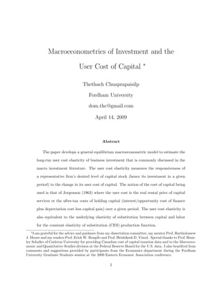
  • 21. Figure 1: United States data. All variables are in logs. 4 Data for VECM estimation The data used in this study are aggregate time-series data for the United States and Canada that represent a large and a small open-economy respectively. The data set consists of quar- terly time series on the variables zt for the period between 1962q4 and 2006q2. A description of data sources and the calculation of the user cost variable is given in Appendix C. 5 Univariate Unit-Root Tests Prior to estimating the VECM (26) or (27), the first step in the analysis is to ascertain whether the data suggest that the variables in zt are integrated of order one, I(1) and are cointegrated with similar cointegration ranks as the number of long-run reduced form theoretical relationships postulated in section 3.1. The augmented Dickey-Fuller (ADF) test results for individual time series of the variables in zt are given in Tables 1 and 2 for the U.S. and Canadian data respectively for the maximum augmented lag length of four and effective 21
  • 22. Figure 2: United States data in first differences. Figure 3: Canadian data. All variables are in logs. 22
  • 23. Figure 4: Canadian data in first differences. sample size of 172 from 1963q3 to 2006q2. The null hypothesis of a unit root, H0 : β = 0, cannot be rejected for most variables at the optimal lag length chosen according to the significance of the longest lag difference coefficient and the Akaike Information Criterion (AIC). The unit root null is rejected for the log of output (yt, yb, yc), employment (lt), consumption (ct) and net export (nxt) series in the U.S. data, and capital stock (kt), user cost (Rt) and short-term real returns (rrp t ) in the Canadian data however. Even though the unit root hypothesis is rejected for these series, most of the estimated ˆβ coefficients are close to zero and the implied AR coefficients (= 1 + ˆβ) are close to one suggesting near unit-root processes. Thus it may be the case that the ADF test has low power against the stationary alternative and is unable to distinguish a stochastic trend from the linear trend for these series. The Dickey-Fuller GLS (DF-GLS) test due to Elliott et al. (1996) which uses a generalized least square procedure to detrend the series has higher power than the standard ADF test.14 The DF-GLS test results in Table 3 and 4 suggest that the unit root null, 14 See Maddala and Kim (1998) and Pfaff (2006) for more description of the DF-GLS and related tests. 23
  • 24. Table 1: ADF unit root tests for the U.S. data. lt yt yb yc wt kt kc t ko t Test statistic -3.520* -4.363** -4.306** -4.176** -1.765 -2.559 -2.479 -2.940 1 + ˆβ 0.94900 0.89550 0.88637 0.89710 0.98818 0.99530 0.99360 0.99689 Lag length 1 2 2 2 3 3 3 3 Rt Rc t Ro t ct nxt rrp t gt Test statistic -1.867 -2.833 -2.583 -4.091** -3.134* -2.548 -2.921 1 + ˆβ 0.96364 0.93117 0.93218 0.92563 0.93793 0.92458 0.95373 Lag length 4 4 4 3 4 3 4 United States Data. ADF regressions: ∆yt = α + µt + βyt−1 + γ1∆yt−1 + . . . + γk∆yt−k + ut. Exclude time trend in the regressions of Ro t and nxt. Critical values derived from the response surfaces in MacKinnon (1991): 5% = −3.44, 1% = −4.01 with a constant and time trend; 5% = −2.88, 1% = −3.47 without time trend, for an effective sample size of 172, 1963q3- 2006q2. Optimal lag length, k chosen according to the AIC and significance of the last lagged difference with a maximum of 4 lags. Table 2: ADF unit root tests for Canadian data. lt yt wt kt Rt Test statistic -2.834 -2.903 -0.9327 -5.215** -4.074** 1 + ˆβ 0.95656 0.96552 0.98416 0.98281 0.63690 Lag length 1 1 4 1 2 ct nxt rrp t gt Test statistic -2.386 -2.287 -3.273* -3.034 1 + ˆβ 0.97280 0.93758 0.70794 0.97218 Lag length 3 0 3 4 Canadian Data. ADF regressions: ∆yt = α + µt + βyt−1 + γ1∆yt−1 + . . . + γk∆yt−k + ut. Exclude time trend in the regressions of nxt and rrp t . Critical values derived from the response surfaces in MacKinnon (1991): 5% = −3.44, 1% = −4.01 with a constant and time trend; 5% = −2.88, 1% = −3.47 without time trend, for an effective sample size of 172, 1963q3-2006q2. Optimal lag length, k chosen according to the AIC and significance of the last lagged difference with a maximum of 4 lags. 24
  • 25. Table 3: ADF-GLS unit root tests for the U.S. data. lt yt yb yc wt kt kc t ko t Test statistic -2.0426 -1.47362 -1.89296 -1.21192 -1.46407 -2.4472 -2.2497 -1.11017 1 + ˆα0 0.9794 0.9835 0.9733 0.9863 0.9930 0.9956 0.9954 0.9991 Lag length 1 2 2 2 3 3 3 3 Rt Rc t Ro t ct nxt rrp t gt Test statistic -1.89878 -2.65464 -2.46817 -1.62595 -2.98335* -2.10471 -2.26166 1 + ˆα0 0.9637 0.9377 0.9398 0.9835 0.9434 0.9439 0.9703 Lag length 4 4 4 3 4 3 4 United States data. ADF-GLS regressions: ∆yd t = α0yd t−1 + α1∆yd t−1 + . . . + αk∆yd t−k + εt where yd t is the locally detrended series of yt with a constant, a linear time trend based on the coefficients from auxiliary regressions. Critical values: 10% = −2.64, 5% = −2.93, 2.5% = −3.18, 1% = −3.46 for effective sample size of 172, 1963q3-2006q2. Optimal lag length, k chosen according to the significance of the last lagged difference with a maximum of 4 lags. Table 4: ADF-GLS unit root tests for Canadian data. lt yt wt kt Rt Test statistic -1.81334 -0.703825 -0.792521 -5.30459** -4.05417** 1 + ˆα0 0.97804 0.99467 0.98892 0.98276 0.64674 Lag length 1 1 4 1 2 ct nxt rrp t gt Test statistic -1.08944 -2.34524 -3.42775* -0.494054 1 + ˆα0 0.99085 0.93750 0.683445 0.99669 Lag length 3 0 3 4 Canadian Data. ADF-GLS regressions: ∆yd t = α0yd t−1 + α1∆yd t−1 + . . . + αk∆yd t−k + εt where yd t is the locally detrended series of yt with a constant, a linear time trend based on the coefficients from auxiliary regressions. Critical values: 10% = −2.64, 5% = −2.93, 2.5% = −3.18, 1% = −3.46 for effective sample size of 172, 1963q3-2006q2. Optimal lag length, k chosen according to the significance of the last lagged difference with a maximum of 4 lags. 25
  • 26. H0 : α0 = 0, can now be accepted for most series. For the U.S. data, only net export (nxt) exhibits some stationarity as the unit root null is weakly rejected at 5% significance level. The implied AR coefficients (= 1 + ˆβ) is close to one however so nxt is likely to be a near unit-root process with a substantial degree of non-stationarity remaining. The unit root null is rejected for the capital stock (kt), user cost (Rt) and short-term real returns (rrp t ) series in the Canadian data still and any remaining non-stationarity has to instead be associated with the vector process involving all variables in a multivariate setting as described in the next section. Unit roots tests can be applied further to the variable in its difference format, ∆yt to see whether the differenced series is I(1) hence whether the original time series is I(2) i.e. whether the original time series, yt can be described by a stochastic process with two unit roots for its distributed lag polynomial and needs to be differenced twice to become weakly stationary. The ADF test results for the variables in their differences are give in Tables 5 and 6 for the United States and Canadian data respectively. The unit root null hypothesis is rejected for almost all the differenced series suggesting that the corresponding level series are at most I(1). The only series that seems to be integrated of order two, I(2) is the high-tech capital stock series kc t in the U.S. data. Other capital stock series for the U.S. also exhibit some degree of I(2)ness with the implied AR coefficients (= 1 + ˆβ) closer to one for the differenced series but the unit root null is rejected at 5% significance level. With the exception of high-tech capital stock kc t , the variables series can therefore be taken as being I(1) overall and incorporated into the VECM of section 3.2. 6 Johansen’s Maximum Likelihood Estimation and Cointegration Rank Tests In a multivariate setting, cointegration rank tests are used to ascertain whether the vector of nine variables, zt = (lt, yt, wt, kt, Rt, ct, nxt, rrt, gt) in section 3.2 can instead be described 26
  • 27. Table 5: ADF unit root tests for the U.S. data in first differences. ∆lt ∆yt ∆yb ∆yc ∆wt ∆kt ∆kc t ∆ko t Test statistic -6.320** -6.640** -6.769** -7.090** -3.826** -3.553** -2.628 -3.119* 1 + ˆβ 0.61175 0.38669 0.36679 0.28727 0.68388 0.93218 0.95257 0.94348 Lag length 0 1 1 1 4 2 2 2 ∆Rt ∆Rc t ∆Ro t ∆ct ∆nxt ∆rrp t ∆gt Test statistic -5.802** -5.552** -10.84** -4.900** -4.306** -7.596** -3.927** 1 + ˆβ 0.17565 0.21956 0.16510 0.48754 0.45151 -0.062973 0.52386 Lag length 3 3 0 2 3 2 3 United States Data. ADF regressions: ∆2 yt = α + β∆yt−1 + γ1∆2 yt−1 + . . . + γk∆2 yt−k + ut. Critical values derived from the response surfaces in MacKinnon (1991): 5% = −2.88, 1% = −3.47 for an effective sample size of 165, 1965q2-2006q2. Optimal lag length, k chosen according to the AIC and significance of the last lagged difference with a maximum of 4 lags. Table 6: ADF unit root tests for Canadian data in first differences. ∆lt ∆yt ∆wt ∆kt ∆Rt Test statistic -8.000** -5.585** -4.509** -3.944** -9.978** 1 + ˆβ 0.43568 0.34776 0.34039 0.88846 -1.5386 Lag length 0 4 3 3 3 ∆ct ∆nxt ∆rrp t ∆gt Test statistic -5.103** -12.30** -12.37** -4.600** 1 + ˆβ 0.38007 0.042431 -1.2816 0.33421 Lag length 2 0 2 3 Canadian Data. ADF regressions: ∆2 yt = α + β∆yt−1 + γ1∆2 yt−1 + . . . + γk∆2 yt−k +ut. Critical values derived from the response surfaces in MacKinnon (1991): 5% = −2.88, 1% = −3.47 for an effective sample size of 165, 1965q2- 2006q2. Optimal lag length, k chosen according to the AIC and significance of the last lagged difference with a maximum of 4 lags. 27
  • 28. by a stationary vector autoregressive (VAR) process with all the roots of its characteristic polynomial lying outside the unit circle i.e. zt ∼ I(0) and the Π matrix in the VEC repre- sentation (26) is of full rank, or whether the vector process is non-stationary I(1) with 9 − r unit roots and r cointegration relations for the 9 × 9 matrix, Π of rank r. Given that the series of the variables in zt have the order of integration of at most one i.e. difference-stationary, Johansen (1988, 1991) and Johansen and Juselius (1990) provide a maximum likelihood procedure to estimate β in the matrix Π = αβ of the VECM (26) under a Guassian distributional assumption for vt, and derive a likelihood ratio (LR) test to determine the number unit roots and the number of cointegration relations in the data.15 The estimation process starts with the Frisch-Waugh regressions of ∆zt and zt−1 on lagged differences ∆zt−1, ∆zt−2, . . . , ∆zt−p+1 and any deterministic or exogenous terms outside the cointegration relations in order to concentrate out the short-run transitory effects.16 The two n × 1 vectors of residuals from the regressions, r0t and r1t respectively, result in the concentrated model r0t = Πr1t + εt (28) which summarizes low-frequency adjustments towards the long-run cointegration relations. Under the distributional assumption of multivariate normality, εt ∼ Nn (0, Ω), the con- centrated log likelihood function for (28) and the data with an effective sample size of T 15 A complete description of the procedure is given in Johansen (1996, Ch. 6) and also in Juselius (2006, Ch. 7), Hamilton (1994, Ch. 20) and Garratt et al. (2006, Ch. 6). The results reported below are from the estimation of β∗ in the matrix Π∗ = αβ∗ in (26) when the trend term is restricted to the cointegration relations. 16 Frisch-Waugh regressions of ∆yt and z∗ t−1 = zt−1, t on ∆gt, ∆zt−1, ∆zt−2, . . . , ∆zt−p+1 and the con- stant term are used for the case of restricted trend and weakly exogenous gt in (27) for the estimation below. 28
  • 29. is lc (Π) = −Tn 2 (1 + ln 2π) − T 2 ln |Ω| = −Tn 2 (1 + ln 2π) − T 2 ln T−1 T t=1 εtεt = −Tn 2 (1 + ln 2π) − T 2 ln T−1 T t=1 (r0t − Πr1t) (r0t − r1tΠ ) = −Tn 2 (1 + ln 2π) − T 2 ln |S00 − ΠS10 − S01Π + ΠS11Π | where S represents the squared correlations, Sij = T−1 T t=1 ritrjt . Unrestricted estimates for Π can be obtained by maximizing the likelihood function or minimizing the sum of squares in the expression above so that ˆΠ = S01 (S11)−1 . The second step of the procedure is to impose a reduced rank restriction Π = αβ and estimate the n × r matrices α and β separately. According to VECM (26), if 0 < r < n then the matrix Π has a reduced rank of r i.e. there are r stationary linear combinations for the variables in zt, β zt that make the level term, Πzt−1 on the right hand side of (26) stationary.17 Since the difference terms are also I(0), the equation as whole is balanced and hence vt in (26) and εt in (28) are stationary.18 The estimation can be done by initially obtaining a maximum likelihood (MLE) or least squares (OLS) estimator of α given β as ˆα (β) = S01β (β S11β) −1 . Then substitute α = ˆα (β) in to the log likelihood function above to obtain ˆlc (β) = −Tn 2 (1 + ln 2π) − T 2 ln S00 − S01β (β S11β) −1 β S10 which can be maximized with respect to β by minimizing the expression for ˆΩ (β) on the 17 The stationary cointegration relations, β zt are taken as long-run reduced form errors ξt in (25) as deviations from the reduced form relations of the macroeconometric model derived in section 3. 18 If r = n then the matrix Π is of full rank and zt is stationary. There is no rank reduction and the VECM represents a VAR model in levels of the stationary variables. If r = 0, on the other hand, then the matrix Π is of zero rank and there is no linear combination of variables in zt that is stationary. The elements in zt represent n individual I(1) processes with no common stochastic trend. An appropriate model is a VAR in first differences instead. 29
  • 30. right-hand side (derived from the formula for a determinant of partition matrices), ˆΩ (β) = S00 − S01β (β S11β) −1 β S10 = |S00| · β S11 − S10S−1 00 S01 β |β S11β| . The optimal choice, ˆβ is obtained by solving the eigenvalue problem |ρN − M| = 0 where M = S11 − S10S−1 00 S01 and N = S11.19 With the resulting n eigenvalues ˆλi = (1 − ˆρi), ˆΩ ˆβ = |S00| n i=1 (1 − ˆλi) (29) and the maximized log likelihood is l∗ c ˆβ = −Tn 2 (1 + ln 2π) − T 2 ln |S00| − T 2 n i=1 ln(1 − ˆλi) Essentially canonical correlation analysis has been applied to the stationary residual vector, r0t and the nonstationary residual vector, r1t to correspond with the stationary error term, εt from the reduced rank regression of (28) when Π = αβ .20 The eigenvalues, ˆλi arranged in descending order, ˆλ1 > . . . > ˆλn ≥ 0 give the squared canonical correlation ˆr2 corr,i between a linear combination of r0t and a linear combination of r1t. Thus the size of the eigenvalue provides a measure of the extent to which the relation, ˆβir1t is correlated with the stationary part of r0t, hence how stationary the long-run cointegration relation ˆβizt−1 is. The number of stationary relations can be determined through cointegration rank tests with the likelihood ratio statistics based on the likelihood function hence the expression for |Ω| in (29). The ‘trace’ statistics, −T n i=r+1 ln(1 − ˆλi) is used to test the null hypothesis, H0 : Rank (Π) = r hence r stationary relations and n − r unit roots against the full rank stationary alternative 19 Since, as pointed out in Juselius (2006) according to Lemma A.8 in Johansen (1996), a function f(x) = |X MX| |X NX| is maximized by solving the eigenvalue problem |ρN − M| = 0. 20 See Johansen (1996, Appendix A) or Hamilton (1994, Ch. 20) for a description of the canonical corre- lation analysis and the motivation for its use in the Johansen’s procedure. 30
  • 31. with no unit roots, H1 : Rank (Π) = n. The statistics is derived as the likelihood ratio, −2 ln Q (H0|H1) = T ln |S00| (1 − ˆλ1)(1 − ˆλ2) · · · (1 − ˆλr) |S00| (1 − ˆλ1)(1 − ˆλ2) · · · (1 − ˆλr) · · · (1 − ˆλn) τn−r = −T ln(1 − ˆλr+1) + · · · + ln(1 − ˆλn) Consecutive tests are applied starting from r = 0 with increasing hypothesized rank when the null is rejected until non-rejection occurs at a particular rank. A similar test can also be done using the ‘maximum eigenvalue’ statistic, −T ln(1 − ˆλr+1) for testing the same null hypothesis against the alternative, H1 : Rank (Π) = r + 1. Unlike the trace test, using the maximum eigenvalue tests in sequence does not lead to a consistent test procedure however. Both statistics have the distribution that is a functional of n − r dimensional Brownian motion under the null hypothesis. The critical values for both tests, also for different cases involving the constant and a trend terms, are given in Johansen and Juselius (1990). Critical values for the cases with weakly exogenous I(1) variables are given in Harbo et al. (1998) and Pesaran et al. (2000). The p-values for the trace test results below are based on the approximations to the asymptotic distributions in Doornik (1998).21 Table 7 gives the trace test result for the United States data for the period between 1962q4 to 2006q2. The null hypothesis of four cointegration relations and four (= 8−4) unit roots is rejected whereas the null of five cointegration relations and three (= 8 − 5) unit roots is not rejected. Therefore the trace test suggests that the long run matrix, Π has a reduced rank of five. The five largest eigenvalues among those that maximize the log-likelihood of (27) are substantially larger than 0.1 and represent nonzero correlations between the corresponding five relations, ˆβir1t and the stationary part of r0t. The trace test results confirm that the five relations, hence the cointegration relations, ˆβizt−1 are stationary. For a given cointegration rank, r the eigenvectors ˆvi corresponding to the r largest non- 21 Cointegration rank tests for an I(2) model are also available with second difference of zt, ∆2 zt placed instead on the left-hand side of the error-correcting equation together with an extra reduced rank condition on the coefficient Γ of ∆zt−1 on the right-hand side. See Rahbek et al. (1999), Paruolo (1996) and Johansen (1995b) for details. 31
  • 32. Table 7: I(1) Cointegration Rank Test for the VECM of (27), 1962q4 to 2006q2. Eigenvalue Log-likelihood for rank 5111.889 0 0.42671 5160.571 1 0.26748 5187.807 2 0.23491 5211.236 3 0.19858 5230.605 4 0.19419 5249.497 5 0.063103 5255.201 6 0.058681 5260.492 7 0.025690 5262.769 8 H0 : rank (Π) ≤ Trace Statistics p-value 0 301.76 [ 0.000 ] ∗∗ 1 204.40 [ 0.000 ] ∗∗ 2 149.93 [ 0.000 ] ∗∗ 3 103.07 [ 0.003 ] ∗∗ 4 64.328 [ 0.044 ] ∗ 5 26.544 [ 0.709 ] 6 15.137 [ 0.570 ] 7 4.5545 [ 0.665 ] Asymptotic p-values based on: Restricted trend and unre- stricted constant. Number of lags used: 2. United States data with gt as a weakly exogenous variable. zero eigenvalues provide a basis for the space of cointegrating vectors each of which can be written as many linear combinations of the eigenvectors; ˆβi = b1 ˆv1 + . . . + br ˆvr, for many different values of scalars, bi. The remaining n − r nonstationary relations, ˆvizt−1 for i = r + 1, . . . , n correspond to the n − r zero eigenvalues. Each cointegrating vector can then be identified by normalizing the eigenvectors ˆV = (ˆv1, . . . , ˆvn) by ˆV S11 ˆV = I according to the Johansen’s statistical identification condition so that ˆβ = (ˆv1, . . . , ˆvr) when ˆβ S11 ˆβ = Ir once normalized and ˆα = S01 ˆβ. Alternatively ˆβ can be identified with the same maximized likelihood value and also over-identified through a set of long-run restrictions on each cointegration relation as described in Johansen (1995a), or according to theoretical restrictions from the long-run reduced form relations in section 3.2 as suggested by Pesaran and Shin (2002) and Garratt, Lee, Pesaran and Shin (2006).22 22 See Boswijk and Doornik (2004) for a review of various identification approaches. 32
  • 33. 7 Estimation of the Long Run Relations The VECM in section 3.2 is estimated here with the VAR lag order of p = 2. The likelihood maximization procedure subject to general linear restrictions is implemented with the PcGive software version 12.10 (Doornik and Hendry, 2007b) which uses Algorithm 4 of Doornik and O’Brien (2002) based on Boswijk (1995) scaled linear switching method.23 The resulting ˆα estimator is asymptotically normally distributed but the estimator for β has a mixed normal limiting distribution with a stochastic variance-covariance matrix. The t-ratios ˆβi/SE ˆβi follow the standard distribution, nonetheless, and can still be used as usual to determine the significance of the maximum likelihood estimates. Long-run coefficient restrictions in the model are also tested as over-identifying restrictions relative to a just-identified model with r2 restrictions imposed.24 Given a cointegration rank of r, the over-identified model, Hc r can be tested against a just-identified alternative, Hr in the stationary I(0) space by using the log-likelihood ratio statistics, −2 ln Λ (Hc r |Hr) = 2 l∗ c ˆθ1 − l∗ c ˆθ0 = T r i=1 ln(1 − ˆλc i ) − r i=1 ln(1 − ˆλi) where l∗ c ˆθ1 and l∗ c ˆθ0 are the maximized log-likelihood values for the just-identified model, Hr and the over-identified model, Hc r respectively. The test statistics has an asymp- totic χ2 distribution with the degrees of freedom depending on the number of over-identifying restrictions.25 23 See Boswijk and Doornik (2004) for a review of various identification approaches and related algorithms to compute maximum likelihood estimates and likelihood ratio statistics. 24 For any non-singular r×r matrix Q, the reduced rank matrix αβ = αQQ−1 β = (αQ) Q−1 β = ˜α ˜β . In addition, any set of coefficient restrictions that results in this rotation of the cointegration space (e.g. normalizing a particular coefficient in the cointegrating vector) will not change the maximized value of the likelihood function regardless of whether there are enough restrictions to achieve identification or not. It is possible however to achieve identification through a rotation of the cointegration space without changing the likelihood value e.g. by normalizing the eigenvectors according to the Johansen’s statistical identification condition or through a set of coefficient restrictions according to Johansen (1995a) or Pesaran and Shin (2002) as mentioned above. 25 The number of over-identifying restrictions is calculated in PcGive using the algorithm of Doornik (1995). Juselius (2006, Ch.12), Boswijk and Doornik (2004) and Pesaran and Shin (2002) also discuss the determination of degrees of freedom. 33
  • 34. The null hypothesis for over-identifying restrictions on β is that the restricted linear combination of the vector process βc i is stationary. If the over-identifying restrictions are rejected when ˆλc i (as the squared canonical correlation coefficients between a linear combi- nation of the stationary part of rc 0t and a linear combination of the non-stationary rc 1t from the vector process ∆zt and zt−1) are small then βc i are seen as being outside the ‘stationary space’ spanned by β for the given rank, r and the restricted cointegration relations, ˆβc i zt are no longer stationary. Since from (29), diag ˆλ1, . . . , ˆλr = ˆβ S10S−1 00 S01 ˆβ = ˆα S−1 00 ˆα once β is normalized according to the Johansen’s identification condition β S11β = Ir above, the rejection of the null hypothesis when ˆλc i are close to zero also implies that ˆαi are not signif- icantly different from zero i.e. the restricted cointegration relations exhibit no statistically significant mean-reversion and there is no equilibrium correction. Weak exogeneity restric- tions on α can also be tested directly using the likelihood ratio test. The null hypothesis for weak exogeneity of a particular variable in zt is that the corresponding row of the α matrix is zero, thereby indicating a lack of error correction feedbacks on the variable. The long-run coefficient estimates for the VECM in section 3.2 using the U.S data is given in Tables 8 and 9. The model contains ten over-identifying restrictions that are strongly re- jected according to the likelihood ratio (LR) test statistics with ten degrees of freedom, χ2 (10) = 56.487 (p-value = 0.0000). Therefore the long-run reduced from theoretical rela- tions as derived in section 3 are altogether too restrictive for the data with their reduced form errors being outside the cointegration space for the given rank. The loss of the cointe- gration property makes the estimated VEC system (27) nonstationary as a whole. This can be seen from the plots of the relations i.e. their long-run reduced form errors in Figure 5. These correspond to ˆβir1t in the model (28) above when the short-run dynamics have been concentrated out. The errors are non-stationary and show no tendency for a correction to- wards the (trend-adjusted) zero means. The cointegration rank test in section 6 above also suggests a rank of 5 thus the nonstationarity for the rank 6 system may also be the result of a unit root that should have been taken as a common stochastic trend driving the vector 34
  • 35. Table 8: Long-run β∗ estimates for the reduced form VECM of (27) with rank(Π∗) = 6 and p = 2, 1962q4 to 2006q2. z∗ t−1 Labor Investment Production IS Consumption YC lt 1.0000 −1.0294 −0.23200 (0.00026580) yt −1.0000 −1.0000 1.0000 1.0000 wt 0.0016102 −0.23200 (0.00036649) (0.036737) kt 1.0000 0.027526 −0.32644 −0.83175 (0.00024531) (0.010583) (0.013684) Rt 0.48238 1.0000 (0.0029620) ct −0.51008 1.0000 (0.020409) nxt −0.036841 (0.0033195) rrp t 0.27746 −0.037431 (0.032959) (0.017517) gt −0.12631 (0.0092347) Trend 0.0029837 −0.0030511 (0.0000342) (0.0000354) United States data. Standard errors in parentheses. Estimated parameters in bold indi- cate significance of the t-ratios at the 0.1% level. Likelihood function maximized under general restrictions based on Doornik (1995) (scaled linear) switching algorithm under weak convergence criterion of |l (θi+1) − l (θi)| ≤ = 0.03. Log-likelihood = 5226.95693. −T/2 ln |Ω| = 7213.47087. Beta is identified and 10 over-identifying restrictions are im- posed. LR test statistics: χ2 (10) = 56.487 [0.0000]∗∗ . Number of observations: 175. Number of parameters: 150. All variables are in logs. kt and Rt are for equipment and software investment. The log short-term real return measure is calculated based on the investment goods price inflation and multiplied by the relative investment goods price so that rrp t = [ln(1 + rt) − πI t+1] × PI t /PY t . 35
  • 36. Table 9: α adjustment coefficient estimates for the reduced form VECM of (27) with rank(Π∗) = 6 and p = 2, 1962q4 to 2006q2. Equation Labor Investment Production IS Consumption YC ∆lt 26.731 −0.62002 26.010 −0.0014817 0.17835 0.29797 (14.818) (0.41212) (14.406) (0.096873) (0.047952) (0.20443) ∆yt 40.890 −1.1025 39.634 −0.30030 0.15664 0.52435 (20.495) (0.57003) (19.926) (0.13399) (0.066324) (0.28276) ∆wt −3.1104 0.098311 −3.0907 −0.010653 0.023089 −0.058989 (9.7598) (0.27145) (9.4887) (0.063806) (0.031583) (0.134654) ∆kt 10.720 −0.26010 10.399 0.082062 0.021830 0.12329 (3.0264) (0.084172) (2.9423) (0.019785) (0.0097935) (0.041753) ∆Rt −469.33 13.076 −456.81 0.63192 −0.076112 −6.5513 (98.646) (2.7436) (95.906) (0.64491) (0.31922) (1.3610) ∆ct 45.143 −1.2438 43.836 0.060003 −0.0072804 0.60300 (19.817) (0.55116) (19.266) (0.12955) (0.064128) (0.27340) ∆nxt −68.902 3.1654 −67.341 1.6565 1.2276 −1.7027 (99.240) (2.7601) (96.483) (0.64879) (0.32115) (1.3692) ∆rrp t 10.785 −0.54028 10.490 −0.0059184 −0.33803 0.27540 (37.549) (1.0443) (36.506) (0.24548) (0.12151) (0.51805) Standard errors in parentheses. Estimated parameters in bold indicate significance of the t-ratios at the 5% level. Long run β∗ and α estimates obtained from the concentrated model (28): r0t = Π∗r1t + εt of the conditional VECM: ∆yt = ay − Π∗z∗ t−1 + Γy1∆zt−1 + ψy0∆gt+uyt where Π∗ = αβ∗. Estimated cointegration relations, ˆβ∗r1 from the preceding table correspond to the following reduced form error correction terms ˆξ ∗ t = ˆβ∗z∗ t−1: ˆξ1,t+1 = lt − yt + 0.0016ωt + 0.0030t Ld ˆξ2,t+1 = kt − yt + 0.48238Rt Investment ˆξ3,t+1 = yt − 1.0294lt + 0.0275kt − 0.0031t Production ˆξ4,t+1 = yt − 0.3264kt − 0.5101ct − 0.0368nxt − 0.1263gt IS ˆξ5,t+1 = ct − 0.2320lt − 0.2320ωt − 0.8318kt + 0.2775rrp t Consumption ˆξ6,t+1 = Rt − 0.0374rrp t Y C . 36
  • 37. Figure 5: Reduced form errors for the long-run relations. Estimated −ˆξt for the VECM (27), 1962q4 to 2006q2. process. The user cost elasticity is precisely estimated at around -0.48 but is likely to be biased due to the nonstationarity of the system. In order to arrive at a cointegrated system that is consistent with the data whilst retaining the structure of the model as much as possible, the next step in the analysis is to find a set of just-identified restrictions on the long-run coefficients such that the cointegration property of the system will still be maintained once some over-identifying restrictions are imposed on the investment equation of interest for the purpose of estimating the user cost elasticity. The just- identifying restrictions are maintained assumptions that resemble the original model guided by theory with some of the original theoretical restrictions being relaxed and still uniquely determine the cointegration vectors. The underlying theoretical relations may still be linear combinations of the cointegration relations and therefore a statistically just-identified model with unique estimates of the coefficients for β may not necessary be identifying in the theoretical sense. Over-identifying restrictions are however imposed to separate out the economic effects as much as possible given the number of cointegration relations hence the 37
  • 38. remaining number of stochastic trends driving the vector process and given the accompanying just-identified model assumptions. Since the trace test in section 6 above suggests a cointegration rank of 5, the analysis proceeds with the estimation of a rank 5 system where the yield curve relation is collapsed and superimposed inside the consumption and investment relations. The two relations now include both the long-term user cost capital, Rt and short-term real returns, rrp t . The short- term real returns, rrp t and weakly exogenous government expenditure, gt are also present in all five relations. These modifications result in a rank 5 system with the following just- identified restrictions, β =             1 −1 β13 0 0 0 −β17 −β18 −β19 0 −1 0 1 β25 0 −β27 −β28 −β29 −β31 1 0 −β34 0 0 0 β38 −β39 0 1 0 −β44 0 −β46 −β47 −β48 −β49 −β51 0 −β51 −β54 −β55 1 0 +β58 −β59             b0 = (b10, b20, b30, b40, b50) and b1 = (b11, b21, b31, 0, 0) so that the long-run reduced form relations become lt = b10 + b11t + yt − β13ωt + β17nxt + β18rrt + β19gt + ξ1,t+1 Ld kt = b20 + b21t + yt − β25Rt + β27nxt + β28rrt + β29gt + ξ2,t+1 Investment yt = b30 + b31t + β31lt + β34kt − β38rrt + β39gt + ξ3,t+1 LRAS yt = b40 + β44kt + β46ct + β47nxt + β48rrt + β49gt + ξ4,t+1 IS ct = b50 + β51lt + β51ωt + β54kt + β55Rt − β58rrt + β59gt + ξ5,t+1 Consumption . Tables 10 and 11 contain the corresponding estimates for an over-identified model with weakly exogenous government expenditure, gt and time trend removed from the investment relation (β29 = 0, b21 = 0). The user cost elasticity estimate under the two over-identifying re- strictions is around -1.91 with net export, nxt still included in the cointegration relation. The 38
  • 39. Table 10: Long-run β∗ estimates for the over-identified VECM of (27) with rank(Π∗) = 5 and p = 2, 1962q4 to 2006q2. z∗ t−1 Labor Investment Production IS Consumption lt 1.0000 −0.85208∗ −0.45304∗ (0.037352) yt −1.0000 −1.0000 1.0000 1.0000 wt 0.12922∗ −0.45304∗ (0.032059) (0.056240) kt 1.0000 −0.26361∗ −0.035386 −0.40647∗ (0.018388) (0.013755) (0.024968) Rt 1.9125∗ −0.22315∗ (0.11895) (0.017498) ct −0.77822∗ 1.0000 (0.026293) nxt −0.067944∗ −1.0111∗ −0.049279∗ (0.0093073) (0.18595) (0.0044202) rrp t −0.26586∗ −6.6812∗ 0.23153∗ −0.10696∗ 0.77444∗ (0.057164) (1.0655) (0.050414) (0.019996) (0.091525) gt 0.073148∗ −0.18590∗ −0.16177∗ −0.23659∗ (0.025286) (0.025986) (0.012769) (0.033603) Trend 0.0028339∗ 0.00065454 (0.00013614) (0.00030597) United States data. Standard errors in parentheses. Estimated parameters in bold indicate significance of the t-ratios at the 5% level and at 1% level with an asterisk. Likelihood function maximized under general restrictions based on Doornik (1995) (scaled linear) switching algorithm under weak convergence criterion of |l (θi+1) − l (θi)| ≤ = 0.005. Log-likelihood = 5247.98759. −T/2 ln |Ω| = 7234.50154. Beta is identified and 2 over- identifying restrictions are imposed. LR test statistics: χ2(2) = 3.0193 [0.2210]. Number of observations: 175. Number of parameters: 151. All variables are in logs. kt and Rt are for equipment and software investment. The log short-term real return measure is calculated based on the investment goods price inflation and multiplied by the relative investment goods price so that rrp t = [ln(1 + rt) − πI t+1] × PI t /PY t . 39
  • 40. Table 11: α adjustment coefficient estimates for the over-identified VECM of (27) with rank(Π∗) = 5 and p = 2, 1962q4 to 2006q2. Equation Labor Investment Production IS Consumption ∆lt −0.066433 0.0095344∗ 0.028934 −0.11145 0.090029 (0.10738) (0.0043023) (0.13117) (0.093880) (0.052082) ∆yt 0.49876∗ −0.010069 0.47283∗ −0.48830∗ −0.088506 (0.15039) (0.0060257) (0.18371) (0.13149) (0.072945) ∆wt 0.078638 −0.0027374 −0.0051453 0.010466 0.017234 (0.071941) (0.0028824) (0.087881) (0.062897) (0.034894) ∆kt 0.077271∗ −0.0028891∗ 0.087255∗ 0.0050440 −0.012648 (0.022138) (0.00088701) (0.027043) (0.019355) (0.010738) ∆Rt −1.9667∗ 0.012601 −3.9010∗ 1.9932∗ 1.3729∗ (0.71329) (0.028579) (0.87134) (0.62362) (0.34597) ∆ct 0.34074∗ −0.0035532 0.35063 −0.0013989 −0.091877 (0.14455) (0.0057918) (0.17658) (0.12638) (0.070114) ∆nxt 0.73140 0.039095 −0.19918 0.91785 0.83582∗ (0.70116) (0.028093) (0.85651) (0.61301) (0.34008) ∆rrp t −0.077447 0.0058118 −0.12361 0.40675 −0.088550 (0.27242) (0.010915) (0.33278) (0.23818) (0.13213) United States data. Standard errors in parentheses. Estimated parameters in bold indicate significance of the t-ratios at the 10% level and at 5% level with an asterisk. Long run β∗ and α estimates obtained from the concentrated model (28): r0t = Π∗r1t + εt of the conditional VECM: ∆yt = ay − Π∗z∗ t−1 + Γy1∆zt−1 + ψy0∆gt + uyt where Π∗ = αβ∗. Estimated cointegration relations, ˆβ∗r1 from the preceding table correspond to the following reduced form error correction terms ˆξ ∗ t = ˆβ∗z∗ t−1: ˆξ1,t+1 = lt − yt + 0.1292ωt − 0.0679nxt − 0.2659rrp t + 0.0731gt + 0.0028t Labor ˆξ2,t+1 = kt − yt + 1.9125Rt − 1.0111nxt − 6.6812rrp t Investment ˆξ3,t+1 = yt − 0.8521lt − 0.2636kt + 0.2315rrp t − 0.1859gt + 0.0007t Production ˆξ4,t+1 = yt − 0.0354kt − 0.7782ct − 0.0493nxt − 0.1070rrp t − 0.1618gt IS ˆξ5,t+1 = ct − 0.4530lt − 0.4530ωt − 0.4065kt − 0.2231Rt + 0.7744rrp t − 0.2366gt Consumption 40
  • 41. Figure 6: Reduced form errors for the long-run relations. Estimated −ˆξt for the over- identified VECM of (27) with rank(Π∗) = 5 and p = 2, 1962q4 to 2006q2. likelihood ratio test of restrictions is not rejected at 20% significance level, χ2 (2) = 3.0193 (p-value = 0.2210). Thus much of the stationarity of the just-identified model is maintained. The cointegration relations that represent long-run reduced form errors for the over-identified rank 5 model are given in figure 6. The errors are now more stationary and adjust frequently towards the zero means. The ADF test for the reduced-formed error for the investment rela- tion, −ˆξ2,t = −(r1k,t−r1y,t+1.9125r1R,t−1.01112r1nx,t−6.6812r1rr,t), where r1i,t are the residu- als from the regressions of yt−1, kt−1, Rt−1, nxt−1 and rrt−1 on ∆gt, ∆zt−1, ∆zt−2, . . . , ∆zt−p+1 and the constant term in (27), in particular, rejects the unit-root null for any lag length including the optimal lag length of one significant lagged difference (and corresponding to most negative Akaike information criterion) at 1% significant level with the t-statistics on the lagged level of -4.029 compared with the 1% critical value of -3.47 (for an effective sample size of 171 from 1963q4 to 2006q2). The ADF(1) test for the relation involving the original vari- able series inclusive of the short-run dynamics, −(kt −yt +1.9125Rt −1.01112nxt −6.6812rrt), also rejects the unit-root null at 1% significant level with the t-statistics on the lagged level 41
  • 42. of -3.999 compared with the 1% critical value of -3.47 (for an effective sample size of 173 from 1963q2 to 2006q2). The likelihood ratio test of zero coefficient restriction for nxt in the investment relation is strongly rejected with the LR statistics, χ2 (3) = 16.865 (p-value = 0.0008). Thus net export can not be excluded from the investment relation without making the cointegration vector pointing outside the stationary cointegration space and resulting in a noncointegrated system. In the theoretical sense, the cointegration relation for investment not only contains the investment first-order condition (8) in section 2 that involves the cointegrating variables {kt, yt, Rt} but also includes demand side relations associated with other cointegration sets involving net exports and these variables e.g. {yt, nxt}, {yt, nxt, kt} or {yt, nxt, Rt}. Since yt and nxt are linked by domestic spending ct, kt and gt given external demand as described by the reduced-form IS relation (18) in section 3.1, the cointegration set {yt, nxt} can be thought of as being influenced by or representing domestic spending and foreign demand. The endogenous components of domestic spending, kt and ct are also related to the user cost variable, Rt through the first-order condition (17) and the consumption and yield curve relation (23) and (24) respectively, resulting in a larger cointegration set {yt, nxt, Rt}. Since the consumption component of domestic spending, ct is also related to the kt component through the consumption relation (23) and since kt also includes imports of foreign capital goods purchased from abroad, the cointegration set {yt, nxt, kt} can also be formed. In fact, from the loading coefficient estimates in Table 11, nxt significantly error corrects only to the long-run reduced form errors in the consumption relation. The investment and consumption relations are therefore likely to be related through net export by a common stochastic trend e.g. domestic and foreign demand shocks that affect the current account. In addition, the loading coefficient estimates in Table 11 also suggest that the user cost of capital, Rt significantly error corrects to all other relations apart from the investment relation itself thus reinforcing the idea that the long-run user cost is an equilibrating variable for the system as a whole and responds to the long-run reduced form shocks including those 42
  • 43. from exogenous policies. The loading coefficient estimates for the short-term real return, rrt on the other hand are not significant for any relations so that rrt is likely to represent monetary policy which only responds to short-run variations in the system.26 Similar long- run estimation results are also obtained if rrt is taken to be weakly exogenous in addition to the government expenditure, gt which represents the role fiscal policy. The trace test for the new system still suggests a cointegration rank of 5 and the over-identifying restrictions are not rejected; LR statistics, χ2 (2) = 3.6192 (p-value = 0.1637) when the model is estimated with otherwise the same set of restrictions as the model where rrt is endogenous. Thus the three stochastic trends in the rank 5 system of eight cointegrating variables and five cointegration relations may be associated with the cumulative trend generated by inter- nal and external demand shocks on the current account and two other trends due to shocks from weakly exogenous monetary and fiscal policies.27 The evidence from the long-run esti- mates therefore suggests that the estimated cointegration relation for investment represents an equilibrium condition that links both the aggregate demand and aggregate supply sides of the model as mentioned towards the end of section 3.1 and that the system as a whole incorporates sufficient structural features of the macroeconomy as described by the model. Although the underlying reduced form relations of the estimated system include other vari- ables that are not previously present in the original reduced form specification in section 3, it is possible to derive them as linear combinations of the original structural relations and new relations that may also explicitly consider, for example, the effects of expected exter- nal demand on firms’ investment decision and of the current account adjustments on the equilibrium interest rate and the long-run user cost of capital. Thus the estimated user cost 26 The test for weak exogeneity of rrt is rejected with LR statistics, χ2 (7) = 32.298 (p-value = 0.0000), however, possibly because of its inclusion in the production relation in the just-identified model. In an alternative model where net export, nxt is included in the production relation instead, the beta cointegration coefficient estimates in other relations are almost identical but different alpha loading coefficients result in a non-rejection of weak exogeneity of rrt with LR statistics, χ2 (7) = 12.161 (p-value = 0.0954). The likelihood ratio test for the weak exogeneity of gt in the rank 5 system, when all variables are endogenous in the cointegration relations with otherwise the same set of over-identifying restrictions, is also not rejected with the LR test statistics, χ2 (7) = 11.497 (p-value = 0.1184). 27 The supply shocks e.g. from technological progress are represented through the restricted trend in the system and will be further explored in the next section when R&D capital is considered. 43
  • 44. elasticity is likely to be influenced by demand-side factors and current account adjustments since net exports is included in the investment relation. Nonetheless, the estimated coeffi- cient of the user cost of capital in the investment relation is consistent with the stationary cointegrated system and represents a stable, albeit biased, estimate of the user cost elasticity from the data within the macroeconometrics framework. The relationship between nxt and yt implied by the estimated cointegration vector for the over-identified model in Table 10 is almost one-to-one so that a reduction in the user cost of capital not only raises the capital-output ratio according to the investment first-order condition but is also associated with a fall in net exports or an increase in the import to export ratio. With a one percent reduction in the user cost and the estimated the user cost elasticity coefficient on Rt of -1.9, the increase in the capital-output ratio will be less than 1.9 percent since net exports is also adjusting; kt − yt − nxt − 6.7rrp t = −1.9Rt. A fall in the user cost is associated with a corresponding fall in the short-term real return and a rise in consumption according to the yield curve and consumption relations. The resulting fall in national savings, in addition to the rise in investment due to the reduction in the user cost, therefore leads to a reduction in net export according to the IS relation (S − I = NX). In other words, the cointegration relation for investment with net export included is an equilibrium relation that combines the structural first-order condition (5) for investment with other relations through net export as explained above and may be written in level of the variables as a [(Yt · NXt)/Kt]1−σ = CK t where NXt = Xt/IMt . An alternative interpretation of the relation is that the marginal product of capital for the production of export goods28 is related to that for the economy as a whole and the relation represents a combination of the corresponding first-order conditions. In addition, net exports, NXt may also include parts of the domestically produced capital stock, e.g. equipment and software in this case, that are produced domestically and exported overseas less imports of 28 Or, more precisely, the ‘marginal product of capital for net exports’ or the ‘marginal product of capital for the ratio of exports to imports’ when nxt is taken as an expenditure based measure of the log of output in the production function of export goods relative to imports. 44
  • 45. Table 12: I(1) Cointegration Rank Test for the VECM of (27) excluding nxt, 1962q4 to 2006q2. Eigenvalue Log-likelihood for rank 4737.943 0 0.28374 4767.143 1 0.24492 4791.725 2 0.21070 4812.427 3 0.17062 4828.797 4 0.092038 4837.245 5 0.057638 4842.439 6 0.026981 4844.833 7 H0 : rank (Π) ≤ Trace Statistics p-value 0 213.78 [ 0.000 ] ∗∗ 1 155.38 [ 0.000 ] ∗∗ 2 106.22 [ 0.000 ] ∗∗ 3 64.811 [ 0.003 ] ∗ 4 32.072 [ 0.044 ] 5 15.176 [ 0.709 ] 6 4.7866 [ 0.570 ] Asymptotic p-values based on: Restricted trend and unrestricted constant. Number of lags used: 2. United States data with seven endogenous variables excluding nxt, and with weakly exogenous gt. foreign capital. A reduction in the user cost of capital encourages firms to retain or import capital stocks for domestic production, resulting in a fall in net exports. More fundamentally, NXt represents excess national savings over investment that does not contribute towards domestic capital accumulation but becomes claims on foreign capital stocks. Thus according to the consumption and yield curve relations in the model, a reduction in the user cost of capital hence the long run short-term real return results in an increase consumption and a fall in national savings, in addition to the rise investment according to the investment first-order condition, that together results in a reduction in the current account balance. If net exports, nxt does not appear explicitly in the model and is excluded from the estimated system altogether, then the trace test suggests a cointegration rank of 4 as shown in Table 12. Long-run estimates for rank 4 systems with either the IS relation (now proxies a current account relationship between excess savings over investment, S − I and the short- 45
  • 46. Table 13: I(1) Cointegration Rank Test for Canadian data 1962q4 to 2006q2. Eigenvalue Log-likelihood for rank 4174.126 0 0.45278 4226.881 1 0.30512 4258.733 2 0.28848 4288.514 3 0.19738 4307.753 4 0.16662 4323.701 5 0.15069 4337.993 6 0.084179 4345.687 7 0.035566 4348.856 8 H0 : rank (Π) ≤ Trace Statistics p-value 0 349.46 [ 0.000 ] ∗∗ 1 243.95 [ 0.000 ] ∗∗ 2 180.25 [ 0.000 ] ∗∗ 3 120.68 [ 0.000 ] ∗∗ 4 82.206 [ 0.000 ] ∗∗ 5 50.309 [ 0.007 ] ∗∗ 6 21.726 [ 0.152 ] 7 6.3374 [ 0.429 ] Asymptotic p-values based on: Restricted trend and unrestricted constant. Number of lags used: 2. Canadian data with weakly exogenous gt and eight endogenous variables. term and long-term real returns on capital) or the consumption relation included are given in Tables 14 and 15 respectively. The estimates for the cointegration vectors are almost identical in both cases with a smaller user cost elasticity estimate of around -0.46, which incidentally is very close to the wage elasticity of -0.42 in the labor demand equation. Time trend and exogenous government expenditure, gt need to be included in the investment relation for stationarity of the system however so the estimated cointegration relation still does not directly correspond to the investment first-order condition. The user cost elasticity estimates are larger at around -1.30 if the trend term is removed from the investment equation and around -1.75 if gt is also removed (whilst the wage elasticity is only slightly smaller at around -0.33) but the overidentifying restrictions hence the stationarity of the system as a whole are strongly rejected in both cases. With the small open-economy Canadian data, an estimate of the user cost elasticity can be obtained from a rank 5 system where net export is not included in the investment 46
  • 47. Table 14: Long-run β∗ and α estimates for the over-identified VECM of (27) with rank(Π∗) = 4 and p = 2 and without nxt in yt, 1962q4 to 2006q2. z∗ t−1 Labor Investment Production IS lt 1.0000 −0.84115∗ (0.047892) yt −1.0000 −1.0000 1.0000 1.0000 wt 0.42059∗ (0.041385) kt 1.0000 −0.26966∗ −0.13429∗ (0.021019) (0.021829) Rt 0.45887∗ −0.096013∗ (0.045718) (0.014433) ct −0.20187∗ −0.64876∗ (0.049111) (0.037625) rrp t −0.14444∗ −1.3773∗ 0.20088∗ 0.18721∗ (0.043405) (0.21307) (0.050320) (0.060569) gt 0.17811∗ 0.49889∗ −0.18698∗ −0.16901∗ (0.027851) (0.091072) (0.028721) (0.023078) Trend 0.0038785∗ −0.0070413∗ 0.00067983 (0.00036321) (0.00048258) (0.00034263) Equation ∆lt −0.14808 −0.047325 0.0050448 −0.20305∗ (0.086039) (0.024962) (0.10074) (0.079725) ∆yt 0.20162 −0.10570∗ 0.11037 −0.49655∗ (0.12116) (0.035151) (0.14186) (0.11227) ∆wt −0.0017314 −0.032634 −0.075266 −0.061118 (0.057734) (0.016750) (0.067599) (0.053497) ∆kt 0.035955∗ −0.0085562 0.041793 −0.0098927 (0.017882) (0.0051878) (0.020937) (0.016569) ∆Rt −1.9863∗ −0.33129∗ −3.3041∗ 1.2843∗ (0.56966) (0.16527) (0.66699) (0.52785) ∆ct 0.13514 −0.013521 0.14285 −0.16105 (0.11846) (0.034369) (0.13871) (0.10977) ∆rrp t −0.0062937 0.14720∗ −0.0052301 0.47495∗ (0.22162) (0.064298) (0.25949) (0.20536) United States data. Standard errors in parentheses. Estimated parameters in bold indicate sig- nificance of the t-ratios at the 10% level and at 5% level with an asterisk. Likelihood function maximized under general restrictions based on Doornik (1995) (scaled linear) switching algorithm under weak convergence criterion of |l (θi+1) − l (θi)| ≤ = 0.005. Log-likelihood = 4828.52228. −T/2 ln |Ω| = 6566.72198. Beta is identified and 1 over-identifying restriction is imposed. LR test statistics: χ2 (1) = 0.54849 [0.4589]. Number of observations: 175. Number of parameters: 117. All variables are in logs. kt and Rt are for equipment and software investment. The log short-term real return measure is calculated based on the investment goods price inflation and multiplied by the relative investment goods price so that rrp t = [ln(1 + rt) − πI t+1] × PI t /PY t . 47
  • 48. Table 15: Long-run β∗ and α estimates for the over-identified VECM of (27) with rank(Π∗) = 4 and p = 2 and without nxt in yt, 1962q4 to 2006q2. z∗ t−1 Labor Investment Production Consumption lt 1.0000 −0.84110∗ −0.52274 (0.042557) yt −1.0000 −1.0000 1.0000 wt 0.42065∗ −0.52274∗ (0.034470) (0.047029) kt 1.0000 −0.26973∗ −0.38164∗ (0.020380) (0.028002) Rt 0.45874∗ −0.24131∗ (0.046123) (0.028084) ct −0.20198∗ 1.0000 (0.035985) rrp t −0.14443∗ −1.3768∗ 0.20081∗ 0.84850∗ (0.042624) (0.21473) (0.049571) (0.12311) gt 0.17813∗ 0.49898∗ −0.18703∗ −0.24913∗ (0.025538) (0.087592) (0.028126) (0.043179) Trend 0.0038793∗ −0.0070423∗ 0.00068082∗ (0.00028251) (0.00047930) (0.00033096) Equation ∆lt 0.070587 0.087643∗ 0.15578 0.17576∗ (0.12627) (0.040171) (0.11718) (0.069076) ∆yt 0.73626∗ 0.22442∗ 0.47878∗ 0.42996∗ (0.17781) (0.056568) (0.16501) (0.097273) ∆wt 0.064032 0.0079375 −0.029891 0.052784 (0.084729) (0.026956) (0.078629) (0.046352) ∆kt 0.046567 −0.0019910 0.049106∗ 0.0085428 (0.026241) (0.0083484) (0.024352) (0.014356) ∆Rt −3.3681∗ −1.1852∗ −4.2564∗ −1.1118∗ (0.83599) (0.26596) (0.77581) (0.45734) ∆ct 0.30842 0.093464 0.26238 0.13920 (0.17385) (0.055309) (0.16134) (0.095107) ∆rrp t −0.51783 −0.16872 −0.35738 −0.41171∗ (0.32524) (0.10347) (0.30182) (0.17792) United States data. Standard errors in parentheses. Estimated parameters in bold indicate sig- nificance of the t-ratios at the 10% level and at 5% level with an asterisk. Likelihood function maximized under general restrictions based on Doornik (1995) (scaled linear) switching algorithm under weak convergence criterion of |l (θi+1) − l (θi)| ≤ = 0.005. Log-likelihood = 4828.5223. −T/2 ln |Ω| = 6566.722. Beta is identified and 1 over-identifying restriction is imposed. LR test statistics: χ2 (1) = 0.54844 [0.4590]. Number of observations: 175. Number of parameters: 117. All variables are in logs. kt and Rt are for equipment and software investment. The log short-term real return measure is calculated based on the investment goods price inflation and multiplied by the relative investment goods price so that rrp t = [ln(1 + rt) − πI t+1] × PI t /PY t . 48
  • 49. relation. Although the trace test suggests a cointegration rank of 6, an overidentified rank 6 system is found to be nonstationary with the likelihood ratio test of the overidentifying restrictions strongly rejected (LR test statistics, χ2 (4) = 24.253, p-value = 0.0001; the estimated user cost elasticity is -1.03). The cointegration estimates from a rank 5 system without net export in the investment relation are shown in Table 16. The user cost elasticity in the investment relation, that now represents the investment first-order condition (given the yield curve relationship between the short-term real returns, rrp t and the long-term user cost, Rt) is around -1.0. The user cost of capital Rt is also weakly exogenous with respect to the investment relation according to the loading adjustment coefficient estimate in Table 17. Capital stock, kt and labor lt are significantly adjusting to the reduced form shocks in the investment relation similar to the estimates from the U.S. data in Table 11. In addition, net exports, now absence from the investment relation, is significantly adjusting to the reduced form error. Thus the cointegration results for the investment relation corresponds to those obtained with the U.S. data in Table 10 and 11 apart from the fact that net exports, nxt can now be excluded from the relation. 8 Conclusion According to the estimation results for the α adjustment coefficients in section 7, the user cost of capital is found to be statistically significantly adjusting to the long-run reduced form shocks on several cointegration relations. Thus there is an evidence that the user cost variable is endogenous to the general equilibrium system and responses to macroeconomic shocks including external and policy shocks.29 The net exports variable is also found to be endogenous to the system. Table 11 shows that net exports respond to reduced form shocks on the modified consumption first-order condition (which also includes long-term user cost and government expenditure). The finding that the estimated investment relation for the 29 In addition, the user cost of capital is weakly exogenous to the long-run investment relation for the VEC system corresponding to the results in Tables 10 and 11 for the U.S. and Tables 16 and 17 for Canada. 49
  • 50. Table 16: Long-run β∗ estimates for the over-identified VECM of (27) with rank(Π∗) = 5 and p = 2, Canadian data 1962q4 to 2006q2. z∗ t−1 Labor Investment Production IS Consumption lt 1.0000 −2.4526∗ −0.47886∗ (0.28171) yt −1.0000 −1.0000 1.0000 1.0000 wt −0.18110 −0.47886∗ (0.11281) (0.10400) kt 1.0000 −0.41987 −0.16184∗ −0.053044 (0.19140) (0.028206) (0.039858) Rt 1.0237∗ 0.43557∗ (0.069226) (0.034454) ct −0.60125∗ 1.0000 (0.063907) nxt 0.35363∗ −0.21744∗ (0.041166) (0.018882) rrp t −0.63196∗ −5.7059∗ −2.0520∗ (0.066922) (0.36297) (0.16556) gt 0.40773∗ −0.19763∗ −0.26531∗ (0.050803) (0.029803) (0.061799) Trend 0.0016387∗ 0.0068328∗ (0.00021170) (0.0017842) Canadian data. Standard errors in parentheses. Estimated parameters in bold indicate significance of the t-ratios at the 5% level and at 1% level with an asterisk. Likelihood function maximized under general restrictions based on Doornik (1995) (scaled linear) switching algorithm under weak convergence criterion of |l (θi+1) − l (θi)| ≤ = 0.005. Log-likelihood = 4317.66804. −T/2 ln |Ω| = 6304.18198. Beta is identified and 6 over- identifying restrictions are imposed. LR test statistics: χ2(6) = 12.067 [0.0605]. Number of observations: 175. Number of parameters: 147. All variables are in logs. kt and Rt are for equipment and machinery investment. The log short-term real return measure is calculated based on the investment goods price inflation and multiplied by the relative investment goods price so that rrp t = [ln(1 + rt) − πI t+1] × PI t /PY t . 50
  • 51. Table 17: α adjustment coefficient estimates for the over-identified VECM of (27) with rank(Π∗) = 5 and p = 2, Canadian data 1962q4 to 2006q2. Equation Labor Investment Production IS Consumption ∆lt 0.038043∗ −0.029045∗ 0.045112∗ −0.045572 0.036723 (0.017648) (0.0098004) (0.010390) (0.048787) (0.025159) ∆yt 0.016385 −0.0045441 0.052714∗ −0.14508∗ −0.036508 (0.024534) (0.013624) (0.014444) (0.067821) (0.034974) ∆wt −0.023522 0.016770 0.011076 −0.059538 −0.044699 (0.035118) (0.019502) (0.020675) (0.097080) (0.050063) ∆kt 0.0066276 −0.0090714∗ 0.0065272 0.0067723 0.021301∗ (0.0055731) (0.0030948) (0.0032811) (0.015406) (0.0079448) ∆Rt 6.1195∗ 0.54378 0.71392 9.8098∗ −4.5350∗ (1.0008) (0.55576) (0.58920) (2.7666) (1.4267) ∆ct −0.018345 −0.011282 0.070811∗ 0.0053904 0.015186 (0.026811) (0.014889) (0.015784) (0.074116) (0.038220) ∆nxt −0.48545∗ 0.35068∗ 0.018205 1.0022∗ −0.79496∗ (0.088445) (0.049115) (0.052071) (0.24450) (0.12608) ∆rrp t 1.2046∗ 0.14321 0.034443 1.9025∗ −0.64865∗ (0.21803) (0.12108) (0.12836) (0.60272) (0.31081) Canadian data. Standard errors in parentheses. Estimated parameters in bold indicate significance of the t-ratios at the 10% level and at 5% level with an asterisk. Long run β∗ and α estimates obtained from the concentrated model (28): r0t = Π∗r1t + εt of the conditional VECM: ∆yt = ay − Π∗z∗ t−1 + Γy1∆zt−1 + ψy0∆gt + uyt where Π∗ = αβ∗. Estimated cointegration relations, ˆβ∗r1 from the preceding table correspond to the following reduced form error correction terms ˆξ ∗ t = ˆβ∗z∗ t−1: ˆξ1,t+1 = lt − yt − 0.1811ωt + 0.3536nxt − 0.6320rrp t + 0.4077gt + 0.0016t Labor ˆξ2,t+1 = kt − yt + 1.0237Rt − 5.7059rrp t Investment ˆξ3,t+1 = yt − 2.4526lt − 0.4199kt + 0.0068t Production ˆξ4,t+1 = yt − 0.1618kt − 0.6012ct − 0.2174nxt − 0.1976gt IS ˆξ5,t+1 = ct − 0.4789lt − 0.4789ωt − 0.0530kt + 0.4356Rt − 2.0520rrp t − 0.2653gt Consumption 51
  • 52. U.S. needs to include net exports in order to maintain the cointegration property of the VECM can be taken as an evidence for the influence of domestic savings and investment on the equilibrium long-term real interest hence on the endogenous user cost of capital in a large open economy. The inclusion of net export prevents a direct interpretation of the investment relation as the first-order condition for investment from which the user cost elasticity can be derived however. The large estimated user cost elasticities for equipment and software capital that are obtained from the investment relation (of around -1.9 according to Table 10 and as summarized in Table 21 below) may be biased since the cointegration relation also takes into account the equilibrium current account adjustment. If net exports variable is removed from the VEC system and linear time trend and weakly exogenous government expenditure is included in the investment relation for cointegration instead then the estimated user cost elasticities fall substantially to around -0.46 as shown in Tables 14 and 15. In an extension to the model of this study (Chuaprapaisilp, 2009, Ch. 5) if the time trend and weakly exogenous government expenditure in the investment relation are replaced by R&D capital stock, assuming capital augmenting R&D technology that makes the real wage weakly exogenous to the system, then small user cost elasticity estimates are also obtained. For most of these cases without the net exports variable in the system, the estimated user cost elasticity in the investment relation is larger (at around -1.1 to -1.3) if time trend or the technology capital variable is removed from the investment relation but cointegration is strongly rejected based on the likelihood ratio test. The VECM estimates for Canada as a small open economy in Table 16, in contrast, result in a user cost elasticity of around one. No additional variables other than short-term real returns need to be included included in the investment relation in order to maintain the cointegration property of the system. An application of similar cointegration techniques to the Canadian data confirm the small open-economy result. Table 18 gives the single equation dynamic OLS (DOLS) estimates of the user cost elasticity based on the empirical 52