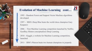
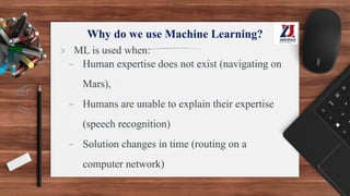
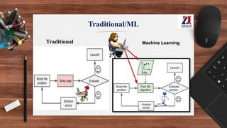
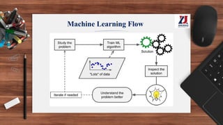
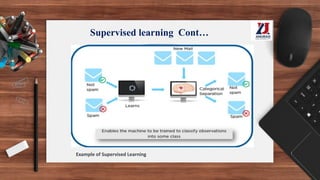
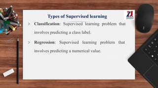
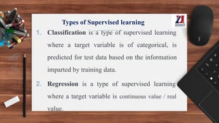
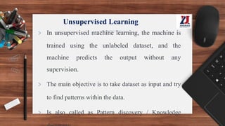
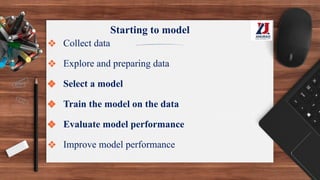
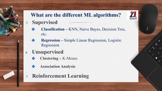
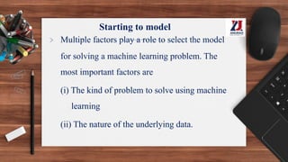
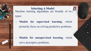
Machine Learning
Unit-I
Mrs. B. Ujwala,
Asst. Professor
What is Learning?
▪ “The process of gaining knowledge and expertise.”
From The Adult Learner by Malcolm Knowles
▪ “A process that leads to change, which occurs as a
result of experience and increases the potential of
improved performance and future learning.”
From How Learning Works: Seven Research-Based
Principles for Smart Teaching by Susan Ambrose, et al.
What is Machine Learning?
Informal Definition: Arthur Samuel, Scientist, StanfordLab
▪ Machine Learning is the field of study that gives computers
the ability to learn without being explicitly programmed.
Formal Definition : Tom Mitchell, Professor of ML Dept,
Carnegie Mellon University
▪ A computer program is said to learn from experience (E)
with respect to some class of task (T) and some
performance measure (P), if its performance at tasks in T,
as measured by P, improves with experience E.
What is Machine Learning? Cont…
In general, to have a well-defined learning problem, we must
identify the following:
1. Class of task
2. Performance measurement that needs to be improved
3. Source of experience
Example: Robot navigation in a maze
Class of task: Reaching the end of the maze
Performance measurement: Time taken to reach the end of the maze
Source of experience: Navigating the maze from start to finish by the
robot
Evolution of Machine Learning
▪ 1950 – Alan Turing proposes “Learning Machine”
▪ 1952 – Arthur Samuel developed first Machine Learning program
that cloud play Checkers
▪ 1957 – Frank Rosenblatt designed the first neural network program
▪ 1967 – Nearest Neighbor algorithm created
▪ 1979 – Stanford University students develop first self-driving cart
that can navigate and avoid obstacles in a room
▪ 1982 – Recurrent Neural Network developed
▪ 1989 – Reinforcement Learning Conceptualized; Beginning of
commercialization of ML
Evolution of Machine Learning cont…
▪ 1995 – Random Forest and Support Vector Machine algorithms
developed
▪ 1997 – IBM’s Deep Blue beats the world chess champion Gary
Kasparov
▪ 2006 – First Machine Learning competition launched by Netflix;
Geoffrey Hinton conceptualizes Deep Learning
▪ 2010 – Kaggle, a website for Machine Learning competition,
launched
▪ 2011– IBM’s Watson beats two human champions in jeopardy
▪ 2016 – Google’s AlphaGo Program beats professional human
player
Why do we use Machine Learning?
> ML is used when:
- Human expertise does not exist (navigating on
Mars),
- Humans are unable to explain their expertise
(speech recognition)
- Solution changes in time (routing on a
computer network)
Traditional/ML
Traditional Machine Learning
Machine Learning Flow
Types of Machine Learning
> Machine learning can be classified into 3 types of
algorithms.
1. Supervised Learning
2. Unsupervised Learning
3. Reinforcement
Types of Machine Learning
Supervised learning
> In Supervised learning, the system is presented with
data which is labeled, and based on the training, the
machine predicts the output.
> The main goal of the supervised learning technique
is to map the input variable(x) with the output
variable(y).
> Some real-world applications of supervised learning
are weather prediction, sales forecasting, stock price
Labeled Data
Supervised learning Cont…
Example of Supervised Learning
Types of Supervised learning
> Classification: Supervised learning problem that
involves predicting a class label.
> Regression: Supervised learning problem that
involves predicting a numerical value.
Types of Supervised learning
1. Classification is a type of supervised learning
where a target variable is of categorical, is
predicted for test data based on the information
imparted by training data.
2. Regression is a type of supervised learning
where a target variable is continuous value / real
value.
Unsupervised Learning
> In unsupervised machine learning, the machine is
trained using the unlabeled dataset, and the
machine predicts the output without any
supervision.
> The main objective is to take dataset as input and try
to find patterns within the data.
> Is also called as Pattern discovery / Knowledge
Unsupervised Learning
Example of Unsupervised Learning
Unsupervised Learning
Example of Unsupervised Learning
Types of Unsupervised learning
1. Clustering or cluster analysis is a machine learning
technique, which groups the unlabelled dataset.
It can be defined as "A way of grouping the data
points into different clusters, consisting of similar
data points. The objects with the possible
similarities remain in a group that has less or no
similarities with another group.”
Types of Unsupervised learning
The clustering technique can be widely used in various
tasks. Some most common uses of this technique are:
> Social network analysis
> Image segmentation
> Anomaly detection, etc.
Types of Unsupervised learning
2. Association: Association learning is a rule
based machine learning that finds important
relations between variables or features in a data set. ,
such as people that buy X also tend to buy Y.
Reinforcement Learning
▪ Reinforcement learning describes a class of problems
where an agent operates in an environment and
must learn to operate using feedback.
▪ Reinforcement learning follows trial and error method
to get the desired result.
Reinforcement Learning
> Reinforcement learning problems are reward-based.
For every task or for every step completed, there will
be a reward received by the agent. If the task is not
achieved correctly, there will be some penalty added.
> An example of a reinforcement problem is playing a
game where the agent has the goal of getting a high
score and can make moves in the game and received
feedback in terms of punishments or rewards.
Reinforcement Learning
The agent observes the environment, takes an action to interact with
the environment, and receives positive or negative reward.
Reinforcement Learning
Example of Reinforcement Learning
Reinforcement Learning
> AlphaGo used RL to defeat the best human Go player.
> RL is an effective tool for personalized online marketing. It
considers the demographic details and browsing history of
the user real-time to show most relevant advertisements.
Reinforcement Learning
> Reinforcement learning algorithms are widely used in
the gaming industries to build games. It is also used
to train robots to do human tasks.
Machine Learning Applications
1. Traffic Alerts - Google Maps
2. Social Media - Automatic Friend Tagging Suggestions in
Facebook (face detection and Image recognition)
3. Transportation and Commuting – Uber & Ola
4. Products Recommendations - 35% of Amazon’s revenue
is generated by Product Recommendations.
Machine Learning Applications
5. Virtual Personal Assistants – (Speech Recognition,
Speech to Text Conversion, Natural Language Processing,
Text to Speech Conversion)
6. Self Driving Cars - Tesla
7. Dynamic Pricing
8. Google Translate
9. Online Video Streaming
10. Fraud Detection
Detailed Machine Learning Process
Preparing to
Model
Input
Data
Refine
d
Data
Learning
Performance
Evaluation
Performance
Improvement
Ste
p 1
Ste
p 2
Ste
p 3
Ste
p 4
Machine Learning Steps
1. Collecting Data
2. Preparing the Data
3. Choosing a Model
4. Training the Model
5. Evaluating the Model
6. Parameter Tuning
7. Making Predictions
Preparing to Model
Learning
Performance Evaluation
Performance Improvement
Machine Learning Activities
Activities in ML
Preparing to Model
The following are the preparation activities done once the input
data comes into the ML system:
▪ Understand the type of data
▪ Explore the data to understand data quality
▪ Explore the relationships amongst the data
▪ Find potential issues in data
▪ Remediate data, if needed
▪ Apply following pre-processing steps
Dimensionality reduction
Feature subset selection
BASIC TYPES OF DATA IN MACHINE LEARNING
• A dataset is a collection of related information or records
• Each row of a dataset is called a record
• Each dataset also has multiple attributes also termed as feature,
variable, dimension
• Example datasets on students
BASIC TYPES OF DATA
Data types can be categorized broadly into two types
1. Qualitative data (also called Categorical data) –
Information which can’t be measured
i. Nominal data is one which has no numeric value– Nationality, Blood
group, Gender...
ii. Ordinal data can be arranged in a sequence – Grade, Satisfaction
level
2. Quantitative data (also called Numeric data) – Information
which can be measured
i. Interval data is numeric data for which not only the order is
known, but the exact difference between values is also known.
Eg:Body temperature
ii. Ratio data is numeric data for which exact value can be
measured. Eg: Age, Weight
Exploring structure of data
> Standard dataset may have the data dictionary, which is a
metadata repository
> With the understanding of the data set attributes, we can
start exploring the numeric and categorical attributes
separately
Exploring numerical data – use box plot and histogram
> Understand the central tendency –
- Mean
- Median
- Mode
> Understand data spread
Data Exploration – central tendency
Mean vs. Median for Auto MPG
Data Exploration – Data spread
> Consider the data values of two attributes
- Attribute 1 values – 44, 46, 48, 45 and 47
- Attribute 2 values – 34, 46, 59, 39 and 52
> Both the set of values have a mean and median of 46.
> First set of values is more concentrated or clustered
around the mean / median value
Data Exploration – data value position
> Any data set attribute has five values
- Minimum
- First quartile (Q1)
- Median (Q2)
- Third quartile (Q3), and
- Maximum
Minimum Maximum
Median
(Q2)
Q3
Q1
Plotting and exploring numerical data
Box plot is an effective mechanism to get one-shot
view and understand the nature of the data
Histogram is an effective visualization plot, which
helps in understanding the distribution of numeric
data into series of intervals, also termed as ‘bins’
Data Exploration – Box plot
Data Exploration – Histogram
Histogram of mpg Histogram of cylinders Histogram of displacement
Histogram of weight Histogram of acceleration Histogram of model.year
Histogram of origin Histogram of horsepower
Exploring relationship between variables
> Scatter plot – shows the relationship between
two variables
> Two-way cross-tabulations(cross-tabs) are
used to understand the relationship of two
categorical attributes in concise way
> It has a matrix format that represents a
summarized view of the bi-variate frequency
distribution
Data Exploration – Scatter plot
Data Exploration – Cross-tabs
Data Quality
> Most occurring data quality issues are:
- Missing values
- Outliers
Missing values of attribute “horsepower” in Auto MPG
Remediate data issues
> Remove missing values / outliers – If number of records
are not many, remove them.
> Imputation - Impute the value with mean or median or
mode
> Capping - In this technique, we cap our outliers data and
make the limit i.e, above a particular value or less than that
value, all the values will be considered as outliers, and the
number of outliers in the dataset gives that capping number.
> Estimate missing values – Assign attribute values of
Other Pre-processing Steps
> Dimensionality reduction
- Principal component analysis (PCA)
- Singular Value Decomposition (SVD)
- Linear Discriminant Analysis (LDA)
> Feature subset selection achieved by
- Removing irrelevant features
- Selecting a subset of potentially redundant
features
Modeling and Evaluation
ML Process
> Basic learning process can be divided into three parts:
1. Data Input
2. Abstraction – gives the summarized and structured
format, such that meaningful insight is obtained from
data
3. Generalization
> This structured representation of raw input data to
the meaningful pattern is called a model.
> The process of assigning a model, and fitting a specific
model to a data set is called model training.
What is modeling in context of machine learning?
> Modelling is the process of selecting and applying an
algorithm for solving a machine learning problem.
> A machine learning algorithm creates its cognitive
capability by building a mathematical formulation or
function, known as target function, based on the
features in the input data set.
Selecting a Model
Starting to model
❖ Collect data
❖ Explore and preparing data
❖ Select a model
❖ Train the model on the data
❖ Evaluate model performance
❖ Improve model performance
What are the different ML algorithms?
> Supervised
❖ Classification – KNN, Naive Bayes, Decision Tree,
etc.
❖ Regression – Simple Linear Regression, Logistic
Regression
> Unsupervised
❖ Clustering – K-Means
❖ Association Analysis
> Reinforcement Learning
Starting to model
> Multiple factors play a role to select the model
for solving a machine learning problem. The
most important factors are
(i) The kind of problem to solve using machine
learning
(ii) The nature of the underlying data.
Selecting A Model
Machine learning algorithms are broadly of two
types:
> Models for supervised learning, which
primarily focus on solving predictive problems
> Models for unsupervised learning, which
solve descriptive problems.
Selecting a model
Predictive models (supervised)
> The models which are used for prediction of
target features of categorical value are known
as classification models.
> The target feature is known as a class and the
categories to which classes are divided into are
called levels
Selecting a model
> Predictive models (supervised)
❖ Predict the value of a category or class
✔ Problems that can be solved : Prediction of
win/loss, fraudulent transactions, etc.
✔ Examples : k-Nearest Neighbor (kNN), Naïve
Bayes, Decision Tree, etc.
❖ Predict numerical values of the target
✔ Problems that can be solved : Prediction of
revenue growth, rainfall amount, etc,
✔ Examples: Linear Regression, Logistic
Regression, etc.
Selecting a model
Descriptive models
(unsupervised) – used to
describe a dataset or gain insight
from a dataset
❖ Group together similar data
instances
❖ Problems that can be solved:
Customer grouping or
segmentation based on social,
demographic, etc. factors
❖ Most popular model for
clustering is k-Means
Training a Model – Holdout Method
(For Supervised Learning)
Training
Data
Inp
ut
Dat
a
Test
Data
Trained
Model
70% - 80%
20% -
30%
Model
Performance
> Smaller datasets may have the challenges to divide
the data of some of the classes proportionally
amongst training and test datasets
> A special variant of holdout method, called repeated
holdout, is sometimes employed to ensure the
randomness of the composed data sets.
Training a Model – k-Fold Cross-Validation
(For Supervised Learning)
Training a Model
k-Fold Cross-Validation
> In k-fold cross-validation technique, the data set is
divided into k-completely separate random partitions
called folds. It is basically repeated holdout into ‘k’
folds.
> The value of ‘k’in k-fold cross validation can be set to
any number. Two extremely popular approaches are:
1.10-fold cross-validation (10-fold CV)
2.Leave-one-out cross-validation (LOOCV)
k-Fold Cross-Validation
Training a Model K-Fold Cross-Validation
> 10-fold cross-validation is by far the most popular
approach. In this approach, for each of the 10-folds, each
comprising of approximately 10% of the data, one of the
folds is used as the test data for validating model
performance trained based on the remaining 9 folds (or 90%
of the data).
> This is repeated 10 times, once for each of the 10 folds
being used as the test data and the remaining folds as the
training data. The average performance across all folds is
being reported. Figure 3.3 depicts the detailed approach of
selecting the ‘k’folds in k-fold cross-validation.
k-Fold Cross-Validation
Leave-one-out cross-validation
Leave-one-out cross-validation is a special case
of cross-validation where the number of folds equals the
number of instances in the data set. Thus, the learning
algorithm is applied once for each instance, using all other
instances as a training set and using the selected instance as a
single-item test set.
Bootstrap sampling
• Bootstrap sampling or simply bootstrapping is a popular
way to identify training and test data sets from the input
data set. It uses the technique of Simple Random Sampling
with Replacement (SRSWR).
• Bootstrapping randomly picks data instances from the input
data set, with the possibility of the same data instance to be
picked multiple times.
Bootstrap sampling
Lazy vs. Eager learning
> Lazy learning (e.g., instance-based learning): Simply stores
training data (or only minor processing) and waits until it is
given a test tuple
> Eager learning (eg. Decision trees, SVM, NN): Given a set
of training set, constructs a classification model before
receiving new (e.g., test) data to classify
> Lazy learning : less time in training but more time in
predicting Accuracy
Model Representation and Interpretability
> Target function of a model is the function defining the
relationship between the input (also called predictor or
independent) variables and the output (also called
response or dependent or target) variable.
> It is represented in the general form: Y = f (X) + e,
where Y is the output variable, X represents the input
variables and ‘e’ is a random error term.
> Fitness of a target function approximated by a learning
algorithm determines how correctly it is able to classify
Model Overfitting and Underfitting
> Underfitting: is a situation when your model is too
simple for your data. More formally, your hypothesis about
data distribution is wrong and too simple — for example,
your data is quadratic and your model is linear. This situation
is also called high bias.
> Underfitting may occurs:
i. When trying to represent a non-linear data with a linear model
ii. Due to unavailability of sufficient training data.
> Underfitting results in both poor performance with training
Model Overfitting and Underfitting
> Overfitting is a situation when your model is too
complex for your data. More formally, your hypothesis about
data distribution is wrong and too complex — for example,
your data is linear and your model is high-degree
polynomial. This situation is also called high variance..
> Overfitting, in many cases, occur as a result of trying to fit
an excessively complex model to closely match the training
data
- Good accuracy on training data but poor on test data
Train a model – Under vs. Over Fit
Und
er
fit
Balan
ced
fit
Ov
er
fit
Und
er
fit
Balan
ced
fit
Ov
er
fit
Bias-Variance Trade-off
> In supervised learning, the class value assigned by
the learning model built based on the training data
may differ from the actual class value.
> This error in learning can be of two types –
1. errors due to ‘bias’
2. error due to ‘variance’
ERRORS DUE TO BIAS
> Errors due to bias arise from simplifying assumptions
made by the model to make the target function less
complex or easier to learn.
> Underfitting results in high bias
Training Set 1 Training Set 2 Training Set 3 Training Set 4
ERRORS DUE TO VARIANCE
> Errors due to variance occur from difference in training data
sets used to train the model.
> Overfitting, results in high variance
Training Set 1 Training Set 2 Training Set 3 Training Set 4
Bias - variance trade-off
> Underfitting: model is too “simple” to represent all
the relevant class characteristics
- High bias and low variance
- High training error and high test error
> Overfitting: model is too “complex” and fits
irrelevant characteristics (noise) in the data
- Low bias and high variance
- Low training error and high test error
Train a model – Bias vs. Variance
EVALUATING PERFORMANCE OF A MODEL
> Based on the number of correct and incorrect
classifications or predictions made by a model, the
accuracy of the model is calculated.
> There are four possibilities with regards to the cricket
match win/loss prediction:
1. The model predicted win and the team won - True Positive (TP)
2. The model predicted win and the team lost - False Positive (FP)
3. The model predicted loss and the team won - False Negative (FN)
4. The model predicted loss and the team lost - True Negative (TN)
Evaluating a model (classification)
> For any classification model, model accuracy is given by total
number of correct classifications (either as the class of interest,
i.e. True Positive or as not the class of interest, i.e. True
Negative) divided by total number of classifications done.
> A matrix containing correct and incorrect predictions in the
form of TPs, FPs, FNs and TNs is known as confusion matrix.
Evaluating a model (classification)
Actual
Win
Actual
Loss
Predicted
Win 85 4
Predicted
Loss 2 9
Model accuracy =
=
=
= 0.94 or 94%
Evaluating a model (classification)
> The percentage of misclassifications is indicated using error
rate which is measured as
> In context of the previous confusion matrix,
Evaluating a model (classification)
> Some measures of model performance which are more important than
accuracy.
Evaluating a model (regression)
Evaluating a model (clustering)
“Clustering is in the eye of the beholder”
> Internal evaluation
- Silhouette width
> External evaluation
- Purity
Evaluating a model (clustering)
a
i1
a
i2
ain
_1
Cluster 1
Cluster 2
Cluster 3
Cluster 4
b14
(1)
b14
(2)
b14
(
n4
)
Silhouette width calculation
si·loh·et
Thank You

MachineLearning_Unit-I.pptx.pdtegfdxcdsfxf

  • 1.
    Machine Learning Unit-I Mrs. B.Ujwala, Asst. Professor
  • 2.
    What is Learning? ▪“The process of gaining knowledge and expertise.” From The Adult Learner by Malcolm Knowles ▪ “A process that leads to change, which occurs as a result of experience and increases the potential of improved performance and future learning.” From How Learning Works: Seven Research-Based Principles for Smart Teaching by Susan Ambrose, et al.
  • 3.
    What is MachineLearning? Informal Definition: Arthur Samuel, Scientist, StanfordLab ▪ Machine Learning is the field of study that gives computers the ability to learn without being explicitly programmed. Formal Definition : Tom Mitchell, Professor of ML Dept, Carnegie Mellon University ▪ A computer program is said to learn from experience (E) with respect to some class of task (T) and some performance measure (P), if its performance at tasks in T, as measured by P, improves with experience E.
  • 4.
    What is MachineLearning? Cont… In general, to have a well-defined learning problem, we must identify the following: 1. Class of task 2. Performance measurement that needs to be improved 3. Source of experience Example: Robot navigation in a maze Class of task: Reaching the end of the maze Performance measurement: Time taken to reach the end of the maze Source of experience: Navigating the maze from start to finish by the robot
  • 5.
    Evolution of MachineLearning ▪ 1950 – Alan Turing proposes “Learning Machine” ▪ 1952 – Arthur Samuel developed first Machine Learning program that cloud play Checkers ▪ 1957 – Frank Rosenblatt designed the first neural network program ▪ 1967 – Nearest Neighbor algorithm created ▪ 1979 – Stanford University students develop first self-driving cart that can navigate and avoid obstacles in a room ▪ 1982 – Recurrent Neural Network developed ▪ 1989 – Reinforcement Learning Conceptualized; Beginning of commercialization of ML
  • 6.
    Evolution of MachineLearning cont… ▪ 1995 – Random Forest and Support Vector Machine algorithms developed ▪ 1997 – IBM’s Deep Blue beats the world chess champion Gary Kasparov ▪ 2006 – First Machine Learning competition launched by Netflix; Geoffrey Hinton conceptualizes Deep Learning ▪ 2010 – Kaggle, a website for Machine Learning competition, launched ▪ 2011– IBM’s Watson beats two human champions in jeopardy ▪ 2016 – Google’s AlphaGo Program beats professional human player
  • 7.
    Why do weuse Machine Learning? > ML is used when: - Human expertise does not exist (navigating on Mars), - Humans are unable to explain their expertise (speech recognition) - Solution changes in time (routing on a computer network)
  • 8.
  • 9.
  • 10.
    Types of MachineLearning > Machine learning can be classified into 3 types of algorithms. 1. Supervised Learning 2. Unsupervised Learning 3. Reinforcement
  • 11.
  • 12.
    Supervised learning > InSupervised learning, the system is presented with data which is labeled, and based on the training, the machine predicts the output. > The main goal of the supervised learning technique is to map the input variable(x) with the output variable(y). > Some real-world applications of supervised learning are weather prediction, sales forecasting, stock price
  • 13.
  • 14.
  • 15.
    Types of Supervisedlearning > Classification: Supervised learning problem that involves predicting a class label. > Regression: Supervised learning problem that involves predicting a numerical value.
  • 16.
    Types of Supervisedlearning 1. Classification is a type of supervised learning where a target variable is of categorical, is predicted for test data based on the information imparted by training data. 2. Regression is a type of supervised learning where a target variable is continuous value / real value.
  • 17.
    Unsupervised Learning > Inunsupervised machine learning, the machine is trained using the unlabeled dataset, and the machine predicts the output without any supervision. > The main objective is to take dataset as input and try to find patterns within the data. > Is also called as Pattern discovery / Knowledge
  • 18.
    Unsupervised Learning Example ofUnsupervised Learning
  • 19.
    Unsupervised Learning Example ofUnsupervised Learning
  • 20.
    Types of Unsupervisedlearning 1. Clustering or cluster analysis is a machine learning technique, which groups the unlabelled dataset. It can be defined as "A way of grouping the data points into different clusters, consisting of similar data points. The objects with the possible similarities remain in a group that has less or no similarities with another group.”
  • 21.
    Types of Unsupervisedlearning The clustering technique can be widely used in various tasks. Some most common uses of this technique are: > Social network analysis > Image segmentation > Anomaly detection, etc.
  • 22.
    Types of Unsupervisedlearning 2. Association: Association learning is a rule based machine learning that finds important relations between variables or features in a data set. , such as people that buy X also tend to buy Y.
  • 23.
    Reinforcement Learning ▪ Reinforcementlearning describes a class of problems where an agent operates in an environment and must learn to operate using feedback. ▪ Reinforcement learning follows trial and error method to get the desired result.
  • 24.
    Reinforcement Learning > Reinforcementlearning problems are reward-based. For every task or for every step completed, there will be a reward received by the agent. If the task is not achieved correctly, there will be some penalty added. > An example of a reinforcement problem is playing a game where the agent has the goal of getting a high score and can make moves in the game and received feedback in terms of punishments or rewards.
  • 25.
    Reinforcement Learning The agentobserves the environment, takes an action to interact with the environment, and receives positive or negative reward.
  • 26.
    Reinforcement Learning Example ofReinforcement Learning
  • 27.
    Reinforcement Learning > AlphaGoused RL to defeat the best human Go player. > RL is an effective tool for personalized online marketing. It considers the demographic details and browsing history of the user real-time to show most relevant advertisements.
  • 28.
    Reinforcement Learning > Reinforcementlearning algorithms are widely used in the gaming industries to build games. It is also used to train robots to do human tasks.
  • 29.
    Machine Learning Applications 1.Traffic Alerts - Google Maps 2. Social Media - Automatic Friend Tagging Suggestions in Facebook (face detection and Image recognition) 3. Transportation and Commuting – Uber & Ola 4. Products Recommendations - 35% of Amazon’s revenue is generated by Product Recommendations.
  • 30.
    Machine Learning Applications 5.Virtual Personal Assistants – (Speech Recognition, Speech to Text Conversion, Natural Language Processing, Text to Speech Conversion) 6. Self Driving Cars - Tesla 7. Dynamic Pricing 8. Google Translate 9. Online Video Streaming 10. Fraud Detection
  • 31.
    Detailed Machine LearningProcess Preparing to Model Input Data Refine d Data Learning Performance Evaluation Performance Improvement Ste p 1 Ste p 2 Ste p 3 Ste p 4
  • 32.
    Machine Learning Steps 1.Collecting Data 2. Preparing the Data 3. Choosing a Model 4. Training the Model 5. Evaluating the Model 6. Parameter Tuning 7. Making Predictions Preparing to Model Learning Performance Evaluation Performance Improvement
  • 33.
  • 34.
    Preparing to Model Thefollowing are the preparation activities done once the input data comes into the ML system: ▪ Understand the type of data ▪ Explore the data to understand data quality ▪ Explore the relationships amongst the data ▪ Find potential issues in data ▪ Remediate data, if needed ▪ Apply following pre-processing steps Dimensionality reduction Feature subset selection
  • 35.
    BASIC TYPES OFDATA IN MACHINE LEARNING • A dataset is a collection of related information or records • Each row of a dataset is called a record • Each dataset also has multiple attributes also termed as feature, variable, dimension • Example datasets on students
  • 37.
    BASIC TYPES OFDATA Data types can be categorized broadly into two types 1. Qualitative data (also called Categorical data) – Information which can’t be measured i. Nominal data is one which has no numeric value– Nationality, Blood group, Gender... ii. Ordinal data can be arranged in a sequence – Grade, Satisfaction level 2. Quantitative data (also called Numeric data) – Information which can be measured i. Interval data is numeric data for which not only the order is known, but the exact difference between values is also known. Eg:Body temperature ii. Ratio data is numeric data for which exact value can be measured. Eg: Age, Weight
  • 38.
    Exploring structure ofdata > Standard dataset may have the data dictionary, which is a metadata repository > With the understanding of the data set attributes, we can start exploring the numeric and categorical attributes separately Exploring numerical data – use box plot and histogram > Understand the central tendency – - Mean - Median - Mode > Understand data spread
  • 39.
    Data Exploration –central tendency Mean vs. Median for Auto MPG
  • 40.
    Data Exploration –Data spread > Consider the data values of two attributes - Attribute 1 values – 44, 46, 48, 45 and 47 - Attribute 2 values – 34, 46, 59, 39 and 52 > Both the set of values have a mean and median of 46. > First set of values is more concentrated or clustered around the mean / median value
  • 41.
    Data Exploration –data value position > Any data set attribute has five values - Minimum - First quartile (Q1) - Median (Q2) - Third quartile (Q3), and - Maximum Minimum Maximum Median (Q2) Q3 Q1
  • 42.
    Plotting and exploringnumerical data Box plot is an effective mechanism to get one-shot view and understand the nature of the data Histogram is an effective visualization plot, which helps in understanding the distribution of numeric data into series of intervals, also termed as ‘bins’
  • 43.
  • 44.
    Data Exploration –Histogram Histogram of mpg Histogram of cylinders Histogram of displacement Histogram of weight Histogram of acceleration Histogram of model.year Histogram of origin Histogram of horsepower
  • 45.
    Exploring relationship betweenvariables > Scatter plot – shows the relationship between two variables > Two-way cross-tabulations(cross-tabs) are used to understand the relationship of two categorical attributes in concise way > It has a matrix format that represents a summarized view of the bi-variate frequency distribution
  • 46.
  • 47.
  • 48.
    Data Quality > Mostoccurring data quality issues are: - Missing values - Outliers Missing values of attribute “horsepower” in Auto MPG
  • 49.
    Remediate data issues >Remove missing values / outliers – If number of records are not many, remove them. > Imputation - Impute the value with mean or median or mode > Capping - In this technique, we cap our outliers data and make the limit i.e, above a particular value or less than that value, all the values will be considered as outliers, and the number of outliers in the dataset gives that capping number. > Estimate missing values – Assign attribute values of
  • 50.
    Other Pre-processing Steps >Dimensionality reduction - Principal component analysis (PCA) - Singular Value Decomposition (SVD) - Linear Discriminant Analysis (LDA) > Feature subset selection achieved by - Removing irrelevant features - Selecting a subset of potentially redundant features
  • 51.
  • 52.
  • 53.
    > Basic learningprocess can be divided into three parts: 1. Data Input 2. Abstraction – gives the summarized and structured format, such that meaningful insight is obtained from data 3. Generalization > This structured representation of raw input data to the meaningful pattern is called a model. > The process of assigning a model, and fitting a specific model to a data set is called model training.
  • 54.
    What is modelingin context of machine learning? > Modelling is the process of selecting and applying an algorithm for solving a machine learning problem. > A machine learning algorithm creates its cognitive capability by building a mathematical formulation or function, known as target function, based on the features in the input data set.
  • 55.
  • 56.
    Starting to model ❖Collect data ❖ Explore and preparing data ❖ Select a model ❖ Train the model on the data ❖ Evaluate model performance ❖ Improve model performance
  • 57.
    What are thedifferent ML algorithms? > Supervised ❖ Classification – KNN, Naive Bayes, Decision Tree, etc. ❖ Regression – Simple Linear Regression, Logistic Regression > Unsupervised ❖ Clustering – K-Means ❖ Association Analysis > Reinforcement Learning
  • 58.
    Starting to model >Multiple factors play a role to select the model for solving a machine learning problem. The most important factors are (i) The kind of problem to solve using machine learning (ii) The nature of the underlying data.
  • 59.
    Selecting A Model Machinelearning algorithms are broadly of two types: > Models for supervised learning, which primarily focus on solving predictive problems > Models for unsupervised learning, which solve descriptive problems.
  • 60.
    Selecting a model Predictivemodels (supervised) > The models which are used for prediction of target features of categorical value are known as classification models. > The target feature is known as a class and the categories to which classes are divided into are called levels
  • 61.
    Selecting a model >Predictive models (supervised) ❖ Predict the value of a category or class ✔ Problems that can be solved : Prediction of win/loss, fraudulent transactions, etc. ✔ Examples : k-Nearest Neighbor (kNN), Naïve Bayes, Decision Tree, etc. ❖ Predict numerical values of the target ✔ Problems that can be solved : Prediction of revenue growth, rainfall amount, etc, ✔ Examples: Linear Regression, Logistic Regression, etc.
  • 62.
    Selecting a model Descriptivemodels (unsupervised) – used to describe a dataset or gain insight from a dataset ❖ Group together similar data instances ❖ Problems that can be solved: Customer grouping or segmentation based on social, demographic, etc. factors ❖ Most popular model for clustering is k-Means
  • 63.
    Training a Model– Holdout Method (For Supervised Learning) Training Data Inp ut Dat a Test Data Trained Model 70% - 80% 20% - 30% Model Performance
  • 64.
    > Smaller datasetsmay have the challenges to divide the data of some of the classes proportionally amongst training and test datasets > A special variant of holdout method, called repeated holdout, is sometimes employed to ensure the randomness of the composed data sets. Training a Model – k-Fold Cross-Validation (For Supervised Learning)
  • 65.
    Training a Model k-FoldCross-Validation > In k-fold cross-validation technique, the data set is divided into k-completely separate random partitions called folds. It is basically repeated holdout into ‘k’ folds. > The value of ‘k’in k-fold cross validation can be set to any number. Two extremely popular approaches are: 1.10-fold cross-validation (10-fold CV) 2.Leave-one-out cross-validation (LOOCV)
  • 66.
  • 67.
    Training a ModelK-Fold Cross-Validation > 10-fold cross-validation is by far the most popular approach. In this approach, for each of the 10-folds, each comprising of approximately 10% of the data, one of the folds is used as the test data for validating model performance trained based on the remaining 9 folds (or 90% of the data). > This is repeated 10 times, once for each of the 10 folds being used as the test data and the remaining folds as the training data. The average performance across all folds is being reported. Figure 3.3 depicts the detailed approach of selecting the ‘k’folds in k-fold cross-validation.
  • 68.
  • 69.
    Leave-one-out cross-validation Leave-one-out cross-validationis a special case of cross-validation where the number of folds equals the number of instances in the data set. Thus, the learning algorithm is applied once for each instance, using all other instances as a training set and using the selected instance as a single-item test set.
  • 70.
    Bootstrap sampling • Bootstrapsampling or simply bootstrapping is a popular way to identify training and test data sets from the input data set. It uses the technique of Simple Random Sampling with Replacement (SRSWR). • Bootstrapping randomly picks data instances from the input data set, with the possibility of the same data instance to be picked multiple times.
  • 71.
  • 72.
    Lazy vs. Eagerlearning > Lazy learning (e.g., instance-based learning): Simply stores training data (or only minor processing) and waits until it is given a test tuple > Eager learning (eg. Decision trees, SVM, NN): Given a set of training set, constructs a classification model before receiving new (e.g., test) data to classify > Lazy learning : less time in training but more time in predicting Accuracy
  • 73.
    Model Representation andInterpretability
  • 74.
    > Target functionof a model is the function defining the relationship between the input (also called predictor or independent) variables and the output (also called response or dependent or target) variable. > It is represented in the general form: Y = f (X) + e, where Y is the output variable, X represents the input variables and ‘e’ is a random error term. > Fitness of a target function approximated by a learning algorithm determines how correctly it is able to classify
  • 75.
    Model Overfitting andUnderfitting > Underfitting: is a situation when your model is too simple for your data. More formally, your hypothesis about data distribution is wrong and too simple — for example, your data is quadratic and your model is linear. This situation is also called high bias. > Underfitting may occurs: i. When trying to represent a non-linear data with a linear model ii. Due to unavailability of sufficient training data. > Underfitting results in both poor performance with training
  • 76.
    Model Overfitting andUnderfitting > Overfitting is a situation when your model is too complex for your data. More formally, your hypothesis about data distribution is wrong and too complex — for example, your data is linear and your model is high-degree polynomial. This situation is also called high variance.. > Overfitting, in many cases, occur as a result of trying to fit an excessively complex model to closely match the training data - Good accuracy on training data but poor on test data
  • 77.
    Train a model– Under vs. Over Fit Und er fit Balan ced fit Ov er fit Und er fit Balan ced fit Ov er fit
  • 78.
    Bias-Variance Trade-off > Insupervised learning, the class value assigned by the learning model built based on the training data may differ from the actual class value. > This error in learning can be of two types – 1. errors due to ‘bias’ 2. error due to ‘variance’
  • 79.
    ERRORS DUE TOBIAS > Errors due to bias arise from simplifying assumptions made by the model to make the target function less complex or easier to learn. > Underfitting results in high bias Training Set 1 Training Set 2 Training Set 3 Training Set 4
  • 80.
    ERRORS DUE TOVARIANCE > Errors due to variance occur from difference in training data sets used to train the model. > Overfitting, results in high variance Training Set 1 Training Set 2 Training Set 3 Training Set 4
  • 81.
    Bias - variancetrade-off > Underfitting: model is too “simple” to represent all the relevant class characteristics - High bias and low variance - High training error and high test error > Overfitting: model is too “complex” and fits irrelevant characteristics (noise) in the data - Low bias and high variance - Low training error and high test error
  • 82.
    Train a model– Bias vs. Variance
  • 83.
  • 84.
    > Based onthe number of correct and incorrect classifications or predictions made by a model, the accuracy of the model is calculated. > There are four possibilities with regards to the cricket match win/loss prediction: 1. The model predicted win and the team won - True Positive (TP) 2. The model predicted win and the team lost - False Positive (FP) 3. The model predicted loss and the team won - False Negative (FN) 4. The model predicted loss and the team lost - True Negative (TN)
  • 85.
    Evaluating a model(classification) > For any classification model, model accuracy is given by total number of correct classifications (either as the class of interest, i.e. True Positive or as not the class of interest, i.e. True Negative) divided by total number of classifications done. > A matrix containing correct and incorrect predictions in the form of TPs, FPs, FNs and TNs is known as confusion matrix.
  • 86.
    Evaluating a model(classification) Actual Win Actual Loss Predicted Win 85 4 Predicted Loss 2 9 Model accuracy = = = = 0.94 or 94%
  • 87.
    Evaluating a model(classification) > The percentage of misclassifications is indicated using error rate which is measured as > In context of the previous confusion matrix,
  • 88.
    Evaluating a model(classification) > Some measures of model performance which are more important than accuracy.
  • 89.
    Evaluating a model(regression)
  • 90.
    Evaluating a model(clustering) “Clustering is in the eye of the beholder” > Internal evaluation - Silhouette width > External evaluation - Purity
  • 91.
    Evaluating a model(clustering) a i1 a i2 ain _1 Cluster 1 Cluster 2 Cluster 3 Cluster 4 b14 (1) b14 (2) b14 ( n4 ) Silhouette width calculation si·loh·et
  • 92.