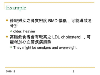
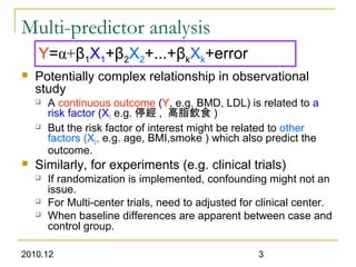
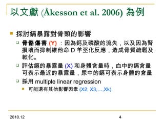
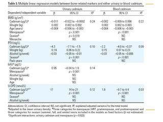
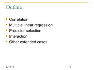
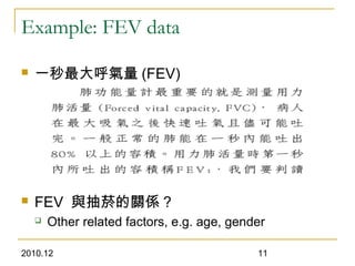
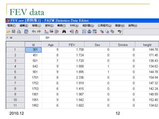
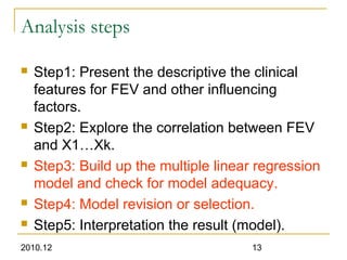
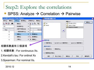
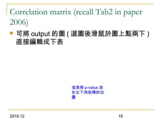
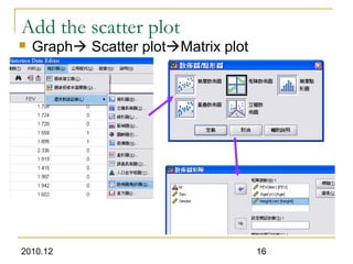
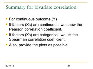
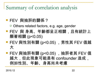
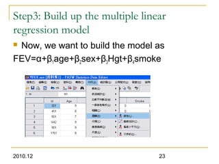
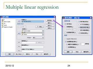
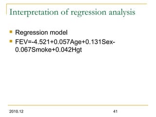
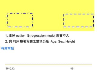
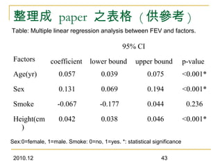
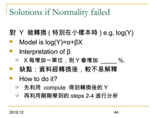
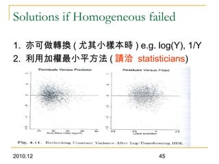
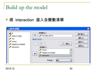
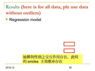
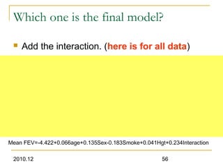
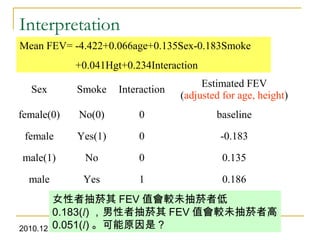
This document discusses using linear regression analysis to explore relationships between variables. It provides an example of using regression to study the relationship between bone mineral density (BMD) and risk factors like menopause and diet. Multiple linear regression allows considering relationships while adjusting for potential confounding factors. The document outlines steps for correlation analysis, building regression models, and checking assumptions. It provides an example analysis of factors related to lung function (FEV) using these steps.

1. 2010.12 1
Linear regression analysis
線性迴歸分析
Wen, shuhui
shwen@mail.tcu.edu.tw
2010.12

2. 2010.12 2
Example
 停經婦女之骨質密度 BMD 偏低，可能導致易
骨折
 older, heavier
 高脂飲食者會有較高之 LDL cholesterol ，可
能增加心血管疾病風險
 They might be smokers and overweight.

3. 2010.12 3
Multi-predictor analysis
 Potentially complex relationship in observational
study
 A continuous outcome (Y, e.g. BMD, LDL) is related to a
risk factor (X1 e.g. 停經 , 高脂飲食 )
 But the risk factor of interest might be related to other
factors (X2, e.g. age, BMI,smoke ) which also predict the
outcome.
 Similarly, for experiments (e.g. clinical trials)
 If randomization is implemented, confounding might not an
issue.
 For Multi-center trials, need to adjusted for clinical center.
 When baseline differences are apparent between case and
control group.
Y=α+β1X1+β2X2+...+βkXk+error

4. 2010.12 4
以文獻 (Åkesson et al. 2006) 為例
 探討鎘暴露對骨頭的影響
 骨骼傷害 (Y) ：因為鈣及磷酸的流失，以及因為腎
損壞而抑制維他命 D 羊巠化反應，造成骨質疏鬆及
軟化。
 評估鎘的暴露量 (X) 和身體含量時，血中的鎘含量
可表示最近的暴露量，尿中的鎘可表示身體的含量
 採用 multiple linear regression
 可能還有其他影響因素 (X2, X3,…,Xk)

5. 2010.12 5
Statistical analyses
 Data from two independent groups of subjects
were compared by the Mann-Whitney U-test. We
used Spearman rank correlation (rs) or Kendall’s
tau to assess univariate associations (p ≤ 0.1). In
multiple linear regression models, each bone-
related variable was evaluated in relation to
cadmium, potential confounders (factors
associated with both cadmium and bone) and
effect modifiers (factors associated with bone).
We explored possible interactions in the model.

6. 2010.12 6
Statistical analyses
Because the season of sampling correlated with blood
and urinary cadmium, BMD, PTH, U-DPD, and
urinary calcium, it was included in the models.
Residual and goodness-of-fit analyses indicated no
deviation from a linear pattern in the regression
models. The final regression model included, apart
from cadmium, only statistically significant variables
(p ≤ 0.05). All tests were two sided, and statistical
evaluation was performed using SPSS (version 12.01;
SPSS Inc., Chicago, IL, USA).

7. 2010.12 7

8. 2010.12 8

9. 2010.12 9

10. 2010.12 10
Outline
 Correlation
 Multiple linear regression
 Predictor selection
 Interaction
 Other extended cases

11. 2010.12 11
Example: FEV data
 一秒最大呼氣量 (FEV)
 FEV 與抽菸的關係 ?
 Other related factors, e.g. age, gender

12. 2010.12 12
FEV data

13. 2010.12 13
Analysis steps
 Step1: Present the descriptive the clinical
features for FEV and other influencing
factors.
 Step2: Explore the correlation between FEV
and X1…Xk.
 Step3: Build up the multiple linear regression
model and check for model adequacy.
 Step4: Model revision or selection.
 Step5: Interpretation the result (model).

14. 2010.12 14
Step2: Explore the correlations
 SPSS: Analyze  Correlation  Pairwise
相關係數處有三個選項
1. 相關係數 : For continuous Xs.
2.Kendall’s tau: For ordinal Xs
3.Spearman: For nominal Xs.

15. 2010.12 15
Correlation matrix (recall Tab2 in paper
2006)
 可將 output 的圖 ( 選圖後滑鼠於圖上點兩下 )
直接編輯成下表
或是將 p-value 放
在左下角矩陣的位
置

16. 2010.12 16
Add the scatter plot
 Graph Scatter plotMatrix plot

17. 2010.12 17
Matrix scatter plot
 散佈圖與相
關係數矩陣
搭配著看
 相關係數看
出正相關且
達顯著
 散佈圖可看
出是否為線
性相關

18. 2010.12 18
For nominal variables, Spearman rs is
more suitable.
 Look at the correlation of FEV and gender(or
smoke)

19. 2010.12 19
Spearman rs
 FEV 與性別 (0=female,1=male) 有關，男性
其 FEV 較大
 FEV 與抽菸 (0=No,1=Yes) 有關，抽菸者其
FEV 較大

20. 2010.12 20
FEV vs. smoke
 抽菸者 FEV
值大 ?
 可能的原因
是抽菸者多
為男性或者
年齡較大 ( 體
型較大 )
 Confounder?

21. 2010.12 21
Summary for bivariate correlation
 For continuous outcome (Y)
 If factors (Xs) are continuous, we show the
Pearson correlation coefficient.
 If factors (Xs) are categorical, we list the
Spearman correlation coefficient.
 Also, provide the plots as possible.

22. 2010.12 22
Summary of correlation analysis
 FEV 與抽菸的關係 ?
 Others related factors, e.g. age, gender
 FEV 與 身高、年齡都呈正相關，且有統計上
顯著相關 (p<0.05)
 FEV 與性別有關 (p<0.05) ，男性其 FEV 值越
大
 FEV 與抽菸有關 (p<0.05) ，抽菸者其 FEV 值
越大，但此現象可能是有 confounder 造成，
例如性別、年齡、身高尚未考慮

23. 2010.12 23
Step3: Build up the multiple linear
regression model
 Now, we want to build the model as
FEV=α+β1age+β2sex+β3Hgt+β4smoke

24. 2010.12 24
Multiple linear regression

25. 2010.12 25
Check for model adequacy.
 點進”圖形”後選擇常態機率圖 ( 為檢驗資料是
否符合常態性假設 )
 畫殘差圖 (Y axis: 殘差值 , X axis:FEV 值 )
 為判斷同質性假設
 若此兩假設不符
則後續檢定迴歸
係數之結果可能
會不對 (not valid)

26. 2010.12 26
Results-1:Pearson Correlation matrix
 除了看出 FEV 與因子 (Xs) 間相關以外， Xs
彼此也有些達統計相關 e.g. age vs. Hgt

27. 2010.12 27
Results-2: Adjusted R-square
 FEV 的變異可被模式中所有因子共同解釋的變
異比例為 0.774 。換句話說，還有 22.6% 為
誤差，可能還有其他影響 FEV 因素未被考慮
。

28. 2010.12 28
Result-3:Collinearity diagnosis( 共線
性 )
 Collinearity: 意指 Xs 彼此高相關而影響 β 值
估計，如此則須再 revise the model.
 檢查指標為 VIF. 若 VIF>10 則表示該變項與
其他變數高相關，可考慮拿掉

29. 2010.12 29
Result-4-1: Normality
 圖中直線若接近
45 度直線則表示
常態性假設成立
 通常 sample size
若夠大可不用太擔
心常態性不成立
 如果常態性不成立
，一般會將 Y 轉換
成 log(Y) 重新做
regression

30. 2010.12 30
Result-4-2: Homogeneous
 正常圖形應該看來
是雜亂無 pattern
 右圖看來有點扇形
(Fan shape) 可能
是違反同質性
 另外 Y-axis 標準化
殘差值落在 (-3,3)
之外的就是異常值

31. 2010.12 31
Outliers
 下表即為 outliers. 一般也可以拿掉後重做
regression. (Do you know how to do it?)

32. 2010.12 32
Influential point
Criterion Bound
Leverage, h >2/n
Studentized residual, r >3
DFFIT >2
Cook's distance >1
High-leverage point could be x-outlier. Influential
point, i.e. one or more β-hat would change by a
large amount.

33. 2010.12 33
Influential point (2)
Reference: Page 122 from Vittinghoff et al. 2005

34. 2010.12 34
Outliers or influential points?
 有 outliers. 無影響點 (max cook’s
distance<1)

35. 2010.12 35
Step4: Model revision or selection.
 根據初步分析結果
 FEV 可被 age, gender, smoke. Height 解釋變異之
比例達 77.4%
 常態性符合，同質性雖不甚符合，但 n 夠大
 無共線性問題，無影響點，有 5 個異常值
 Model revision
 試著將 outliers 去掉後再做一次

36. 2010.12 36
先儲存標準化殘差，再利用 selection
功能將 outlier 去掉
執行完
regression
後請到
資料
選擇觀察值

37. 2010.12 37
Delete outliers and do regression again
 條件為 abs(ZRE_1) <=3

38. 2010.12 38
Interpretation of regression analysis
 重新做 regression 後的結果即可仿照 page
23-33 步驟 檢視統計結果
 N=649 ( 原本有 654 筆 )

39. 2010.12 39
Adjusted R-square (new)
 R-square is 78.7%. A little larger than
previous one.

40. 2010.12 40
Normality, Collinearity, Homogeneous
 Normality 符合
 常態機率圖 接近 45 度直線
 Collinearity
 VIF 皆小於 10, 無共線性
 Homogeneous
 殘差圖與之前一樣
 Outliers
 雖有但很輕微 ( 很接近 3) 故不再排除

41. 2010.12 41
Interpretation of regression analysis
 Regression model
 FEV=-4.521+0.057Age+0.131Sex-
0.067Smoke+0.042Hgt

42. 2010.12 42
1. 拿掉 outlier 後 regression model 影響不大
2. 與 FEV 顯著相關之變項仍是 Age, Sex, Height
有異常點

43. 2010.12 43
整理成 paper 之表格 ( 供參考 )
95% CI
Factors coefficient lower bound upper bound p-value
Age(yr) 0.057 0.039 0.075 <0.001*
Sex 0.131 0.069 0.194 <0.001*
Smoke -0.067 -0.177 0.044 0.236
Height(cm
)
0.042 0.038 0.046 <0.001*
Sex:0=female, 1=male. Smoke: 0=no, 1=yes. *: statistical significance
Table: Multiple linear regression analysis between FEV and factors.

44. 2010.12 44
Solutions if Normality failed
對 Y 做轉換 ( 特別在小樣本時 ) e.g, log(Y)
 Model is log(Y)=α+βX
 Interpretation of β
 X 每增加一單位，則 Y 會增加 _____ %.
 缺點：資料經轉換後，較不易解釋
 How to do it?
 先利用 compute 得到轉換後的 Y
 再利用剛剛學到的 steps 2-4 進行分析

45. 2010.12 45
Solutions if Homogeneous failed
1. 亦可做轉換 ( 尤其小樣本時 ) e.g. log(Y), 1/Y
2. 利用加權最小平方法 ( 請洽 statisticians)

46. 2010.12 46
Solutions if Collinearity exists
 Model selection
 利用模式選取的方式，放入較顯著的變項，以避免
Xs 之間之高相關
 Forward, Backward, Stepwise regression
 Stepwise 較常使用

47. 2010.12 47
Stepwise regression

48. 2010.12 48
Results

49. 2010.12 49
Selected model
Model is FEV=-4.449+0.041Hgt+0.061Age+0.161Sex
(here is for all data, plz use data without outliers)

50. 2010.12 50
Interaction
 若 Z 與 X 對 Y 的交互作用存在，則 Z 的值不
同時， X 與 Y 的關係會改變
 統計角度，可畫出 Y 的 mean plot for each X*Z
group
 模式中要加入 interaction effect, 作法是
 加入 X 與 Z 的交乘項 X*Z ，檢定 X*Z 的迴歸係數
是否為 0 ，若顯著則 X 與 Z 之 interaction 存在

51. 2010.12 51
Sex vs. Smoke?

52. 2010.12 52
Check for mean FEV
由敘述性統計值看來
男生的 FEV 值與女生的 FEV 值之差異會因抽菸狀態不同而不同
可能有交互作用存在 (from statistical viewpoint)
此處尚未考慮 Age, Height 的影響喔，
若加入 confounder 後關係會再改變 !
(Multiple regression)

53. 2010.12 53
Add interaction effects
 檢驗抽菸與性別之交互作用
 1. 先新增加乘項 (name it as “interaction”)

54. 2010.12 54
Build up the model
 將 interaction 選入自變數清單

55. 2010.12 55
Results (here is for all data, plz use data
without outliers)
 Regression model
抽 與性別之交互作用存在，此時菸
的 smoke 主效應亦存在

56. 2010.12 56
Which one is the final model?
 Add the interaction. (here is for all data)
Mean FEV=-4.422+0.066age+0.135Sex-0.183Smoke+0.041Hgt+0.234Interaction

57. 2010.12 57
Interpretation
Sex Smoke Interaction
Estimated FEV
(adjusted for age, height)
female(0) No(0) 0 baseline
female Yes(1) 0 -0.183
male(1) No 0 0.135
male Yes 1 0.186
Mean FEV= -4.422+0.066age+0.135Sex-0.183Smoke
+0.041Hgt+0.234Interaction
女性者抽菸其 FEV 值會較未抽菸者低
0.183(l) ，男性者抽菸其 FEV 值會較未抽菸者高
0.051(l) 。可能原因是 ?

58. 2010.12 58
會是身高影響 ?

59. 2010.12 59
Further issues
 What if Y is not continuous?
 If Y is binary, say disease vs. healthy. Suggest
use the logistic regression (next class by Prof.
Hsieh).
 What if Y are repeated measure, say pre/post
Y?
 Might use post-Y as response variable, and
adjusted for pre-Y and Xs. (For 2 time points)
 For several time points, suggest use “repeated-
measure” ANOVA. ( 請洽 statisticians)

60. 2010.12 60
References
1. M. Pagano, K. Gauvereau. Principles of
Biostatistics(2nd Ed). Australia ; Pacific Grove,
CA : Duxbury, 2000. ( 歐亞書局代理 )
2. Rosner B. (2006) Fundamentals of Biostatistics
(6th ed). Belmont, CA : Thomson-Brooks/Cole ( 歐
亞代理 )
3. Vittinghoff E., Glidden D.V., Shiboski S.C.,
McCulloch C.E. Regression Methods in
Biostatistics. Spreinger 2005.
4. 史麗珠 (2005) ，進階應用生物統計學。學富文化
，台北。