Lecture_3_Mathematics_for_Machine_Learning.pptx

CS 404/504
Special Topics: Adversarial
Machine Learning
Dr. Alex Vakanski

2
CS 404/504, Fall 2021
Lecture 3
Mathematics for Machine Learning

3
CS 404/504, Fall 2021
Lecture Outline
• Linear algebra
 Vectors
 Matrices
 Eigen decomposition
• Differential calculus
• Optimization algorithms
• Probability
 Random variables
 Probability distributions
• Information theory

4
CS 404/504, Fall 2021
Notation
• Scalar (integer or real)
• Vector (bold-font, lower case)
• Matrix (bold-font, upper-case)
• Tensor ((bold-font, upper-case)
• Random variable (normal font, upper-case)
• Set membership: is member of set
• Cardinality: number of items in set
• Norm of vector
• or Dot product of vectors and
• Set of real numbers
• Real numbers space of dimension n
• or Function (map): assign a unique value to each input
value
• Function (map): map an n-dimensional vector into a scalar

5
CS 404/504, Fall 2021
Notation
• Element-wise product of matrices A and B
• Pseudo-inverse of matrix A
• n-th derivative of function f with respect to x
• Gradient of function f with respect to x
• Hessian matrix of function f
• Random variable has distribution
• Probability of given
• Gaussian distribution with mean and variance
• Expectation of with respect to
• Variance of
• Covariance of and
• Correlation coefficient for and
• Kullback-Leibler divergence for distributions and
• Cross-entropy for distributions and

6
CS 404/504, Fall 2021
Vectors
• Vector definition
 Computer science: vector is a one-dimensional array of ordered real-valued scalars
 Mathematics: vector is a quantity possessing both magnitude and direction,
represented by an arrow indicating the direction, and the length of which is
proportional to the magnitude
• Vectors are written in column form or in row form
 Denoted by bold-font lower-case letters
• For a general form vector with elements the vector lies in the -dimensional space
Vectors

7
CS 404/504, Fall 2021
Geometry of Vectors
• First interpretation of a vector: point in space
 E.g., in 2D we can visualize the data points with
respect to a coordinate origin
• Second interpretation of a vector: direction in
space
 E.g., the vector has a direction of 3 steps to the right
and 2 steps up
 The notation is sometimes used to indicate that the
vectors have a direction
 All vectors in the figure have the same direction
• Vector addition
 We add the coordinates, and follow the directions
given by the two vectors that are added
Vectors
Picture from: http://d2l.ai/chapter_appendix-mathematics-for-deep-learning/geometry-linear-algebraic-ops.html#geometry-of-vectors

8
CS 404/504, Fall 2021
Geometry of Vectors
• The geometric interpretation of vectors as points in space allow us to consider a
training set of input examples in ML as a collection of points in space
 Hence, classification can be viewed as discovering how to separate two clusters of
points belonging to different classes (left picture)
o Rather than distinguishing images containing cars, planes, buildings, for example
 Or, it can help to visualize zero-centering and normalization of training data (right
picture)
Vectors

9
CS 404/504, Fall 2021
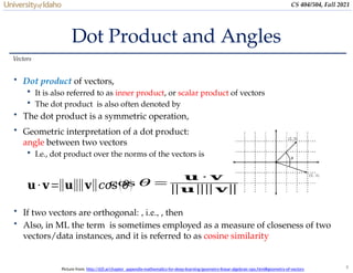
• Geometric interpretation of a dot product:
angle between two vectors
 I.e., dot product over the norms of the vectors is
Dot Product and Angles
• Dot product of vectors,
 It is also referred to as inner product, or scalar product of vectors
 The dot product is also often denoted by
• The dot product is a symmetric operation,
Vectors
𝐮∙ 𝐯=‖𝐮‖‖𝐯‖𝑐𝑜𝑠(𝜃)
cos 𝜃 =
𝐮 ∙ 𝐯
‖𝐮‖
‖𝐯‖
Picture from: http://d2l.ai/chapter_appendix-mathematics-for-deep-learning/geometry-linear-algebraic-ops.html#geometry-of-vectors
• If two vectors are orthogonal: , i.e., , then
• Also, in ML the term is sometimes employed as a measure of closeness of two
vectors/data instances, and it is referred to as cosine similarity

10
CS 404/504, Fall 2021
Norm of a Vector
• A vector norm is a function that maps a vector to a scalar value
 The norm is a measure of the size of the vector
• The norm should satisfy the following properties:
 Scaling:
 Triangle inequality:
 Must be non-negative:
• The general norm of a vector is obtained as:
 On next page we will review the most common norms, obtained for and
Vectors
‖𝐱‖𝑝=
(∑
𝑖=1
𝑛
|𝑥𝑖|
𝑝
)
1
𝑝

11
CS 404/504, Fall 2021
Norm of a Vector
• For we have norm
 Also called Euclidean norm
 It is the most often used norm
 norm is often denoted just as with the subscript 2 omitted
 Uses the absolute values of the elements
 Discriminate between zero and non-zero elements
 Known as infinity norm, or max norm
 Outputs the absolute value of the largest element
• norm outputs the number of non-zero elements
 It is not an norm, and it is not really a norm function either (it is incorrectly called a
norm)
Vectors
‖𝐱‖∞=max
𝑖
|𝑥𝑖|
‖𝐱‖2=
√∑
𝑖=1
𝑛
𝑥𝑖
2
=√𝐱
𝑇
𝐱
‖𝐱‖1 =∑
𝑖=1
𝑛
|𝑥𝑖|

12
CS 404/504, Fall 2021
Vector Projection
• Orthogonal projection of a vector onto vector
 The projection can take place in any space of
dimensionality ≥ 2
 The unit vector in the direction of is
o A unit vector has norm equal to 1
 The length of the projection of onto is
 The orthogonal project is the vector
Vectors
Slide credit: Jeff Howbert — Machine Learning Math Essentials

13
CS 404/504, Fall 2021
Hyperplanes
• Hyperplane is a subspace whose dimension is one less than that of its ambient
space
 In a 2D space, a hyperplane is a straight line (i.e., 1D)
 In a 3D, a hyperplane is a plane (i.e., 2D)
 In a d-dimensional vector space, a hyperplane has dimensions, and divides the space
into two half-spaces
• Hyperplane is a generalization of a concept of plane in high-dimensional space
• In ML, hyperplanes are decision boundaries used for linear classification
 Data points falling on either sides of the hyperplane are attributed to different classes
Hyperplanes
Picture from: https://kgpdag.wordpress.com/2015/08/12/svm-simplified/

14
CS 404/504, Fall 2021
Hyperplanes
• For example, for a given data point , we can use dot-
product to find the hyperplane for which
 I.e., all vectors with can be classified as one class, and
all vectors with can be classified as another class
• Solving , we obtain
 I.e., the solution is the set of points for which meaning
the points lay on the line that is orthogonal to the vector
o That is the line
 The orthogonal projection of onto is
Hyperplanes
𝐰
Picture from: http://d2l.ai/chapter_appendix-mathematics-for-deep-learning/geometry-linear-algebraic-ops.html#hyperplanes

15
CS 404/504, Fall 2021
Hyperplanes
• In a 3D space, if we have a vector and try to find all points that satisfy , we can
obtain a plane that is orthogonal to the vector
 The inequalities and again define the two subspaces that are created by the plane
• The same concept applies to high-dimensional spaces as well
Hyperplanes
Picture from: http://d2l.ai/chapter_appendix-mathematics-for-deep-learning/geometry-linear-algebraic-ops.html#hyperplanes

16
CS 404/504, Fall 2021
Matrices
• Matrix is a rectangular array of real-valued scalars arranged in m horizontal
rows and n vertical columns
 Each element belongs to the ith
row and jth
column
 The elements are denoted or or or
• For the matrix , the size (dimension) is or
 Matrices are denoted by bold-font upper-case letters
Matrices

17
CS 404/504, Fall 2021
Matrices
• Addition or subtraction
• Scalar multiplication
• Matrix multiplication
 Defined only if the number of columns of the left matrix is the same as the number of
rows of the right matrix
 Note that
Matrices
  , ,
, i j i j
i j
  
A B A B
  ,
, i j
i j
c c
 
A A
  ,1 1, ,2 2, , ,
, i j i j i n n j
i j
   
AB A B A B A B


18
CS 404/504, Fall 2021
Matrices
• Transpose of the matrix: has the rows and columns exchanged
 Some properties
• Square matrix: has the same number of rows and columns
• Identity matrix ( In ): has ones on the main diagonal, and zeros elsewhere
 E.g.: identity matrix of size 3×3 :
Matrices
  ,
,
T
j i
i j

A A
3
1 0 0
0 1 0
0 0 1
 
 
 
 
 
I

19
CS 404/504, Fall 2021
Matrices
• Determinant of a matrix, denoted by det(A) or is a real-valued scalar encoding
certain properties of the matrix
 E.g., for a matrix of size 2×2:
 For larger-size matrices the determinant of a matrix id calculated as
 In the above, is a minor of the matrix obtained by removing the row and column
associated with the indices i and j
• Trace of a matrix is the sum of all diagonal elements
• A matrix for which is called a symmetric matrix
Matrices
det
a b
ad bc
c d
 
 
 
 
 
 
 

20
CS 404/504, Fall 2021
Matrices
• Elementwise multiplication of two matrices A and B is called the Hadamard
product or elementwise product
 The math notation is
Matrices

21
CS 404/504, Fall 2021
Matrix-Vector Products
• Consider a matrix and a vector
• The matrix can be written in terms of its row vectors (e.g., is the first row)
• The matrix-vector product is a column vector of length m, whose ith
element is
the dot product
• Note the size:
Matrices

22
CS 404/504, Fall 2021
Matrix-Matrix Products
• To multiply two matrices and
• We can consider the matrix-matrix product as dot-products of rows in and
columns in
• Size:
Matrices

23
CS 404/504, Fall 2021
Linear Dependence
• For the following matrix
• Notice that for the two columns and , we can write
 This means that the two columns are linearly dependent
• The weighted sum is referred to as a linear combination of the vectors and
 In this case, a linear combination of the two vectors exist for which
• A collection of vectors are linearly dependent if there exist coefficients not all
equal to zero, so that
• If there is no linear dependence, the vectors are linearly independent
Matrices
𝐁=
[2 −1
4 − 2]

24
CS 404/504, Fall 2021
Matrix Rank
• For an matrix, the rank of the matrix is the largest number of linearly
independent columns
• The matrix B from the previous example has , since the two columns are linearly
dependent
• The matrix C below has , since it has two linearly independent columns
 I.e., , ,
Matrices
𝐁=
[2 −1
4 − 2]

25
CS 404/504, Fall 2021
Inverse of a Matrix
• For a square matrix A with rank , is its inverse matrix if their product is an
identity matrix I
• Properties of inverse matrices
• If (i.e., ), then the inverse does not exist
 A matrix that is not invertible is called a singular matrix
• Note that finding an inverse of a large matrix is computationally expensive
 In addition, it can lead to numerical instability
• If the inverse of a matrix is equal to its transpose, the matrix is said to be
orthogonal matrix
Matrices
 
 
1
1
1 1 1


  


A A
AB B A
1 T


A A

26
CS 404/504, Fall 2021
Pseudo-Inverse of a Matrix
• Pseudo-inverse of a matrix
 Also known as Moore-Penrose pseudo-inverse
• For matrices that are not square, the inverse does not exist
 Therefore, a pseudo-inverse is used
• If , then the pseudo-inverse is and
• If , then the pseudo-inverse is and
 E.g., for a matrix with dimension , a pseudo-inverse can be found of size , so that
Matrices

27
CS 404/504, Fall 2021
Tensors
• Tensors are n-dimensional arrays of scalars
 Vectors are first-order tensors,
 Matrices are second-order tensors,
 E.g., a fourth-order tensor is
• Tensors are denoted with upper-case letters of a special font face (e.g., )
• RGB images are third-order tensors, i.e., as they are 3-dimensional arrays
 The 3 axes correspond to width, height, and channel
 E.g., 224 × 224 × 3
 The channel axis corresponds to the color channels (red, green, and blue)
Tensors

28
CS 404/504, Fall 2021
Manifolds
• Earlier we learned that hyperplanes generalize the concept of planes in high-
dimensional spaces
 Similarly, manifolds can be informally imagined as generalization of the concept of
surfaces in high-dimensional spaces
• To begin with an intuitive explanation, the surface of the Earth is an example of a
two-dimensional manifold embedded in a three-dimensional space
 This is true because the Earth looks locally flat, so on a small scale it is like a 2-D plane
 However, if we keep walking on the Earth in one direction, we will eventually end up
back where we started
o This means that Earth is not really flat, it only looks locally like a Euclidean plane, but at large
scales it folds up on itself, and has a different global structure than a flat plane
Manifolds

29
CS 404/504, Fall 2021
Manifolds
• Manifolds are studied in mathematics under topological spaces
• An n-dimensional manifold is defined as a topological space with the property
that each point has a neighborhood that is homeomorphic to the Euclidean space
of dimension n
 This means that a manifold locally resembles Euclidean space near each point
 Informally, a Euclidean space is locally smooth, it does not have holes, edges, or other
sudden changes, and it does not have intersecting neighborhoods
 Although the manifolds can have very complex structure on a large scale, resemblance
of the Euclidean space on a small scale allows to apply standard math concepts
Manifolds
• Examples of 2-dimensional manifolds are shown
in the figure
 The surfaces in the figure have been conveniently
cut up into little rectangles that were glued together
 Those small rectangles locally look like flat
Euclidean planes
Picture from: http://bjlkeng.github.io/posts/manifolds/

30
CS 404/504, Fall 2021
Manifolds
• Examples of one-dimensional manifolds
 Upper figure: a circle is a l-D manifold embedded in 2-D,
where each arc of the circle locally resembles a line segment
 Lower figures: other examples of 1-D manifolds
 Note that a number 8 figure is not a manifold because it has
an intersecting point (it is not Euclidean locally)
• It is hypothesized that in the real-world, high-dimensional
data (such as images) lie on low-dimensional manifolds
embedded in the high-dimensional space
 E.g., in ML, let’s assume we have a training set of images with
size pixels
 Learning an arbitrary function in such high-dimensional
space would be intractable
 Despite that, all images of the same class (“cats” for example)
might lie on a low-dimensional manifold
 This allows function learning and image classification
Manifolds
Picture from: http://bjlkeng.github.io/posts/manifolds/

31
CS 404/504, Fall 2021
Manifolds
• Example:
 The data points have 3 dimensions (left figure), i.e., the input space of the data is 3-
dimensional
 The data points lie on a 2-dimensional manifold, shown in the right figure
 Most ML algorithms extract lower-dimensional data features that enable to distinguish
between various classes of high-dimensional input data
o The low-dimensional representations of the input data are called embeddings
Manifolds

32
CS 404/504, Fall 2021
Eigen Decomposition
• Eigen decomposition is decomposing a matrix into a set of eigenvalues and
eigenvectors
• Eigenvalues of a square matrix are scalars and eigenvectors are non-zero
vectors that satisfy
• Eigenvalues are found by solving the following equation
• If a matrix has n linearly independent eigenvectors with corresponding
eigenvalues , the eigen decomposition of is given by
 Columns of the matrix are the eigenvectors, i.e.,
 is a diagonal matrix of the eigenvalues, i.e.,
• To find the inverse of the matrix A, we can use
 This involves simply finding the inverse of a diagonal matrix
Eigen Decomposition

33
CS 404/504, Fall 2021
Eigen Decomposition
• Decomposing a matrix into eigenvalues and eigenvectors allows to analyze
certain properties of the matrix
 If all eigenvalues are positive, the matrix is positive definite
 If all eigenvalues are positive or zero-valued, the matrix is positive semidefinite
 If all eigenvalues are negative or zero-values, the matrix is negative semidefinite
o Positive semidefinite matrices are interesting because they guarantee that ,
• Eigen decomposition can also simplify many linear-algebraic computations
 The determinant of A can be calculated as
 If any of the eigenvalues are zero, the matrix is singular (it does not have an inverse)
• However, not every matrix can be decomposed into eigenvalues and eigenvectors
 Also, in some cases the decomposition may involve complex numbers
 Still, every real symmetric matrix is guaranteed to have an eigen decomposition
according to , where is an orthogonal matrix
Eigen Decomposition

34
CS 404/504, Fall 2021
Eigen Decomposition
• Geometric interpretation of the eigenvalues and eigenvectors is that they allow to
stretch the space in specific directions
 Left figure: the two eigenvectors and are shown for a matrix, where the two vectors
are unit vectors (i.e., they have a length of 1)
 Right figure: the vectors and are multiplied with the eigenvalues and
o We can see how the space is scaled in the direction of the larger eigenvalue
• E.g., this is used for dimensionality reduction with PCA (principal component
analysis) where the eigenvectors corresponding to the largest eigenvalues are
used for extracting the most important data dimensions
Eigen Decomposition
Picture from: Goodfellow (2017) – Deep Learning

35
CS 404/504, Fall 2021
Singular Value Decomposition
• Singular value decomposition (SVD) provides another way to factorize a matrix,
into singular vectors and singular values
 SVD is more generally applicable than eigen decomposition
 Every real matrix has an SVD, but the same is not true of the eigen decomposition
o E.g., if a matrix is not square, the eigen decomposition is not defined, and we must use SVD
• SVD of an matrix is given by
 is an matrix, is an matrix, and is an matrix
 The elements along the diagonal of are known as the singular values of A
 The columns of are known as the left-singular vectors
 The columns of are known as the right-singular vectors
• For a non-square matrix , the squares of the singular values are the eigenvalues
of , i.e., for
• Applications of SVD include computing the pseudo-inverse of non-square
matrices, matrix approximation, determining the matrix rank
Singular Value Decomposition

36
CS 404/504, Fall 2021
Matrix Norms
• Frobenius norm – calculates the square-root of the
summed squares of the elements of matrix
 This norm is similar to Euclidean norm of a vector
• Spectral norm – is the largest singular value of matrix
 Denoted
 The singular values of are ,…,
• norm – is the sum of the Euclidean norms of the
columns of matrix
• Max norm – is the largest element of matrix X
Matrix Norms
‖𝐗‖𝐹=√∑
𝑖=1
𝑚
∑
𝑗=1
𝑛
𝑥𝑖𝑗
2
‖𝐗‖2=𝜎𝑚𝑎𝑥 (𝐗 )
‖𝐗‖2,1=∑
𝑗=1
𝑛
√∑
𝑖=1
𝑚
𝑥𝑖𝑗
2
‖𝐗‖max=max
𝑖 , 𝑗
(𝑥𝑖𝑗 )

37
CS 404/504, Fall 2021
Differential Calculus
• For a function the derivative of f is defined as
• If exists, f is said to be differentiable at a
• If f ‘ is differentiable for , then f is differentiable on this interval
 We can also interpret the derivative as the instantaneous rate of change of with respect
to x
 I.e., for a small change in x, what is the rate of change of
• Given , where x is an independent variable and y is a dependent variable, the
following expressions are equivalent:
• The symbols , D, and are differentiation operators that indicate operation of
differentiation

38
CS 404/504, Fall 2021
• The following rules are used for computing the derivatives of explicit functions

39
CS 404/504, Fall 2021
Higher Order Derivatives
• The derivative of the first derivative of a function is the second derivative of
• The second derivative quantifies how the rate of change of is changing
 E.g., in physics, if the function describes the displacement of an object, the first
derivative gives the velocity of the object (i.e., the rate of change of the position)
 The second derivative gives the acceleration of the object (i.e., the rate of change of the
velocity)
• If we apply the differentiation operation any number of times, we obtain the n-th
derivative of

40
CS 404/504, Fall 2021
Taylor Series
• Taylor series provides a method to approximate any function at a point if we
have the first n derivatives
• For instance, for , the second-order approximation of a function is
• Similarly, the approximation of with a Taylor polynomial of n-degree is
• For example, the figure shows the first-order,
second-order, and fifth-order polynomial of
the exponential function at the point
Picture from: http://d2l.ai/chapter_appendix-mathematics-for-deep-learning/single-variable-calculus.html

41
CS 404/504, Fall 2021
Geometric Interpretation
• To provide a geometric interpretation of the derivatives, let’s consider a first-
order Taylor series approximation of at
• The expression approximates the function by a line which passes through the
point and has slope (i.e., the value of at the point )
• Therefore, the first derivative of a
function is also the slope of the
tangent line to the curve of the
function
Picture from: http://d2l.ai/chapter_appendix-mathematics-for-deep-learning/single-variable-calculus.html

42
CS 404/504, Fall 2021
Partial Derivatives
• So far, we looked at functions of a single variable, where
• Functions that depend on many variables are called multivariate functions
• Let be a multivariate function with n variables
 The input is an n-dimensional vector and the output is a scalar y
 The mapping is
• The partial derivative of y with respect to its ith
parameter is
• To calculate ( pronounced “del” or we can just say “partial derivative”), we can
treat as constants and calculate the derivative of y only with respect to
• For notation of partial derivatives, the following are equivalent:

43
CS 404/504, Fall 2021
Gradient
• We can concatenate partial derivatives of a multivariate function with respect to
all its input variables to obtain the gradient vector of the function
• The gradient of the multivariate function with respect to the n-dimensional
input vector , is a vector of n partial derivatives
• When there is no ambiguity, the notations or are often used for the gradient
instead of
 The symbol for the gradient is the Greek letter (pronounced “nabla”), although is
more often it is pronounced “gradient of f with respect to x”
• In ML, the gradient descent algorithm relies on the opposite direction of the
gradient of the loss function with respect to the model parameters for
minimizing the loss function
 Adversarial examples can be created by adding perturbation in the direction of the
gradient of the loss with respect to input examples for maximizing the loss function

44
CS 404/504, Fall 2021
Hessian Matrix
• To calculate the second-order partial derivatives of multivariate functions, we
need to calculate the derivatives for all combination of input variables
• That is, for a function with an n-dimensional input vector , there are second
partial derivatives for any choice of i and j
• The second partial derivatives are assembled in a matrix called the Hessian
• Computing and storing the Hessian matrix for functions with high-dimensional
inputs can be computationally prohibitive
 E.g., the loss function for a ResNet50 model with approximately 23 million parameters,
has a Hessian of (trillion) parameters

45
CS 404/504, Fall 2021
Jacobian Matrix
• The concept of derivatives can be further generalized to vector-valued functions
(or, vector fields)
• For an n-dimensional input vector , the vector of functions is given as
• The matrix of first-order partial derivates of the vector-valued function is an
matrix called a Jacobian
 For example, in robotics a robot Jacobian matrix gives the partial derivatives of the
translational and angular velocities of the robot end-effector with respect to the joints
(i.e., axes) velocities

46
CS 404/504, Fall 2021
Integral Calculus
• For a function defined on the domain , the definite integral of the function is
denoted
• Geometric interpretation of the integral is the area between the horizontal axis
and the graph of between the points a and b
 In this figure, the integral is the sum of blue areas (where minus the pink area
(where )
Integral Calculus
Picture from: https://mjo.osborne.economics.utoronto.ca/index.php/tutorial/index/1/clc/t

47
CS 404/504, Fall 2021
Optimization
• Optimization is concerned with optimizing an objective function — finding the
value of an argument that minimizes of maximizes the function
 Most optimization algorithms are formulated in terms of minimizing a function
 Maximization is accomplished vie minimizing the negative of an objective function
(e.g., minimize )
 In minimization problems, the objective function is often referred to as a cost function
or loss function or error function
• Optimization is very important for machine learning
 The performance of optimization algorithms affect the model’s training efficiency
• Most optimization problems in machine learning are nonconvex
 Meaning that the loss function is not a convex function
 Nonetheless, the design and analysis of algorithms for solving convex problems has
been very instructive for advancing the field of machine learning
Optimization

48
CS 404/504, Fall 2021
Optimization
• Optimization and machine learning have related, but somewhat different goals
 Goal in optimization: minimize an objective function
o For a set of training examples, reduce the training error
 Goal in ML: find a suitable model, to predict on data examples
o For a set of testing examples, reduce the generalization error
• For a given empirical function g (dashed purple curve), optimization algorithms
attempt to find the point of minimum empirical risk
Optimization
• The expected function f (blue curve) is
obtained given a limited amount of training
data examples
• ML algorithms attempt to find the point of
minimum expected risk, based on minimizing
the error on a set of testing examples
o Which may be at a different location than the
minimum of the training examples
o And which may not be minimal in a formal sense
Picture from: http://d2l.ai/chapter_optimization/optimization-intro.html

49
CS 404/504, Fall 2021
Stationary Points
• Stationary points ( or critical points) of a differentiable function of one variable
are the points where the derivative of the function is zero, i.e.,
• The stationary points can be:
 Minimum, a point where the derivative changes from negative to positive
 Maximum, a point where the derivative changes from positive to negative
 Saddle point, derivative is either positive or negative on both sides of the point
• The minimum and maximum points are collectively known as extremum points
Optimization
• The nature of stationary points can be
determined based on the second derivative
of at the point
 If , the point is a minimum
 If , the point is a maximum
 If , inconclusive, the point can be a saddle
point, but it may not
• The same concept also applies to gradients
of multivariate functions

50
CS 404/504, Fall 2021
Local Minima
• Among the challenges in optimization of model’s parameters in ML involve local
minima, saddle points, vanishing gradients
• For an objective function , if the value at a point x is the minimum of the
objective function over the entire domain of x, then it is the global minimum
• If the value of at x is smaller than the values of the objective function at any
other points in the vicinity of x, then it is the local minimum
Optimization
 The objective functions in ML usually have
many local minima
o When the solution of the optimization
algorithm is near the local minimum, the
gradient of the loss function approaches or
becomes zero (vanishing gradients)
o Therefore, the obtained solution in the final
iteration can be a local minimum, rather than
the global minimum

51
CS 404/504, Fall 2021
Saddle Points
• The gradient of a function at a saddle point is 0, but the point is not a minimum
or maximum point
 The optimization algorithms may stall at saddle points, without reaching a minima
• Note also that the point of a function at which the sign of the curvature changes
is called an inflection point
 An inflection point () can also be a saddle point, but it does not have to be
• For the 2D function (right figure), the saddle point is at (0,0)
 The point looks like a saddle, and gives the minimum with respect to x, and the
maximum with respect to y
Optimization
saddle point
x

52
CS 404/504, Fall 2021
Convex Optimization
• A function of a single variable is concave if every line segment joining two
points on its graph does not lie above the graph at any point
• Symmetrically, a function of a single variable is convex if every line segment
joining two points on its graph does not lie below the graph at any point
Optimization
Picture from: https://mjo.osborne.economics.utoronto.ca/index.php/tutorial/index/1/cv1/t

53
CS 404/504, Fall 2021
Convex Functions
• In mathematical terms, the function fis a convex function if for all points and for
all
Optimization

54
CS 404/504, Fall 2021
Convex Functions
• One important property of convex functions is that they do not have local
minima
 Every local minimum of a convex function is a global minimum
 I.e., every point at which the gradient of a convex function = 0 is the global minimum
 The figure below illustrates two convex functions, and one nonconvex function
Optimization
Picture from: http://d2l.ai/chapter_optimization/convexity.html
convex non-convex convex

55
CS 404/504, Fall 2021
Convex Functions
• Another important property of convex functions is stated by the Jensen’s
inequality
• Namely, if we let and , the definition of convex function becomes
• The Danish mathematician Johan Jensen showed that this can be generalized for
all that are non-negative real numbers a, to the following:
• This inequality is also identical to
 I.e., the expectation of a convex function is larger than the convex function of an
expectation
Optimization

56
CS 404/504, Fall 2021
Convex Sets
• A set in a vector space is a convex set is for any the line segment connecting a
and b is also in
• For all , we have
for all
Optimization
• In the figure, each point represents a 2D vector
 The left set is nonconvex, and the other two sets are convex
• Properties of convex sets include:
 If and are convex sets, then is also convex
 If and are convex sets, then is not necessarily convex

57
CS 404/504, Fall 2021
Derivatives and Convexity
• A twice-differentiable function of a single variable is convex if and only if its
second derivative is non-negative everywhere
 Or, we can write,
 For example, is convex, since , and , meaning that
• A twice-differentiable function of many variables is convex if and only if its
Hessian matrix is positive semi-definite everywhere
 Or, we can write,
 This is equivalent to stating that all eigenvalues of the Hessian matrix are non-negative
(i.e.,
Optimization

58
CS 404/504, Fall 2021
Constrained Optimization
• The optimization problem that involves a set of constraints which need to be
satisfied to optimize the objective function is called constrained optimization
• E.g., for a given objective function and a set of constraint functions
• The points that satisfy the constraints form the feasible region
• Various optimization algorithms have been developed for handling optimization
problems based on whether the constraints are equalities, inequalities, or a
combination of equalities and inequalities
Optimization

59
CS 404/504, Fall 2021
Lagrange Multipliers
• One approach to solving optimization problems is to substitute the initial
problem with optimizing another related function
• The Lagrange function for optimization of the constrained problem on the
previous page is defined as
where
• The variables are called Lagrange multipliers and ensure that the constraints are
properly enforced
 They are chosen just large enough to ensure that
• This is a saddle-point optimization problem where one wants to minimize with
respect to and simultaneously maximize with respect to
 The saddle point of gives the optimal solution to the original constrained optimization
problem
Optimization

60
CS 404/504, Fall 2021
Projections
• An alternative strategy for satisfying constraints are projections
• E.g., gradient clipping in NNs can require that the norm of the gradient is
bounded by a constant value c
• Approach:
 At each iteration during training
 If the norm of the gradient , then the update is
 If the norm of the gradient , then the update is
• Note that since is a unit vector (i.e., it has a norm = 1), then the vector has a
norm =
• Such clipping is the projection of the gradient g onto the ball of radius c
 Projection on the unit ball is for
Optimization

61
CS 404/504, Fall 2021
Projections
• More generally, a projection of a vector onto a set is defined as
• This means that the vector is projected onto the closest vector that belongs to the
set
Optimization
• For example, in the figure, the blue circle represents
a convex set
 The points inside the circle project to itself
o E.g., is the yellow vector, its closest point in the set is i:
the distance between and is
 The points outside the circle project to the closest
point inside the circle
o E.g., is the yellow vector, its closest point in the set is the
red vector
o Among all vectors in the set , the red vector has the
smallest distance to , i.e.,

62
CS 404/504, Fall 2021
First-order vs Second-order Optimization
• First-order optimization algorithms use the gradient of a function for finding
the extrema points
 Methods: gradient descent, proximal algorithms, optimal gradient schemes
 The disadvantage is that they can be slow and inefficient
• Second-order optimization algorithms use the Hessian matrix of a function for
finding the extrema points
 This is since the Hessian matrix holds the second-order partial derivatives
 Methods: Newton’s method, conjugate gradient method, Quasi-Newton method,
Gauss-Newton method, BFGS (Broyden-Fletcher-Goldfarb-Shanno) method,
Levenberg-Marquardt method, Hessian-free method
 The second-order derivatives can be thought of as measuring the curvature of the loss
function
 Recall also that the second-order derivative can be used to determine whether a
stationary points is a maximum , minimum (
 This information is richer than the information provided by the gradient
 Disadvantage: computing the Hessian matrix is computationally expensive, and even
prohibitive for high-dimensional data
Optimization

63
CS 404/504, Fall 2021
Lower Bound and Infimum
• Lower bound of a subset from a partially ordered set is an element of , such that
for all
 E.g., for the subset from the natural numbers , lower bounds are the numbers 2, 1, 0, ,
and all other natural numbers
• Infimum of a subset from a partially ordered set is the greatest lower bound i,
denoted
 It is the maximal quantity such that for all
 E.g., the infimum of the set is 2, since it is the greatest lower bound
• Example: consider the subset of positive real numbers (excluding zero)
 The subset does not have a minimum, because for every small positive number, there
is a another even smaller positive number
 On the other hand, all real negative numbers and 0 are lower bounds on the subset
 0 is the greatest lower bound of all lower bounds, and therefore, the infimum of is 0
Optimization

64
CS 404/504, Fall 2021
Upper Bound and Supremum
• Upper bound of a subset from a partially ordered set is an element of , such that
for all
 E.g., for the subset from the natural numbers , upper bounds are the numbers 8, 9, 40,
and all other natural numbers
• Supremum of a subset from a partially ordered set is the least upper bound i,
denoted
 It is the minimal quantity such that for all
 E.g., the supremum of the subset is , since it is the least upper bound
• Example: for the subset of negative real numbers (excluding zero)
 All real positive numbers and 0 are upper bounds
 0 is the least upper bound, and therefore, the supremum of
Optimization

65
CS 404/504, Fall 2021
Lipschitz Function
• A function is a Lipschitz continuous function if a constant exists, such that for
all points ,
• Such function is also called a -Lipschitz function
• Intuitively, a Lipschitz function cannot change too fast
 I.e., if the points and are close (i.e., the distance is small), that means that the and
are also close (i.e., the distance is also small)
o The smallest real number that bounds the change of for all points , is the Lipschitz constant
of the function
 For a -Lipschitz function , the first derivative is bounded everywhere by
• E.g., the function is 1-Lipschitz over
 Since
 I.e.,
Optimization

66
CS 404/504, Fall 2021
Lipschitz Continuous Gradient
• A differentiable function has a Lipschitz continuous gradient if a constant
exists, such that for all points ,
• For a function with a -Lipschitz gradient, the second derivative is bounded
everywhere by
• E.g., consider the function
 is not a Lipschitz continuous function, since , so when then , i.e., the derivative is not
bounded everywhere
 Since , therefore the gradient is 2-Lipschitz everywhere, since the second derivative is
bounded everywhere by 2
Optimization

67
CS 404/504, Fall 2021
Probability
• Intuition:
 In a process, several outcomes are possible
 When the process is repeated a large number of times, each outcome occurs with a
relative frequency, or probability
 If a particular outcome occurs more often, we say it is more probable
• Probability arises in two contexts
 In actual repeated experiments
o Example: You record the color of 1,000 cars driving by. 57 of them are green. You estimate the
probability of a car being green as 57/1,000 = 0.057.
 In idealized conceptions of a repeated process
o Example: You consider the behavior of an unbiased six-sided die. The expected probability of
rolling a 5 is 1/6 = 0.1667.
o Example: You need a model for how people’s heights are distributed. You choose a normal
distribution to represent the expected relative probabilities.
Probability

68
CS 404/504, Fall 2021
Probability
• Solving machine learning problems requires to deal with uncertain quantities, as
well as with stochastic (non-deterministic) quantities
 Probability theory provides a mathematical framework for representing and
quantifying uncertain quantities
• There are different sources of uncertainty:
 Inherent stochasticity in the system being modeled
o For example, most interpretations of quantum mechanics describe the dynamics of subatomic
particles as being probabilistic
 Incomplete observability
o Even deterministic systems can appear stochastic when we cannot observe all of the variables
that drive the behavior of the system
 Incomplete modeling
o When we use a model that must discard some of the information we have observed, the
discarded information results in uncertainty in the model’s predictions
o E.g., discretization of real-numbered values, dimensionality reduction, etc.
Probability

69
CS 404/504, Fall 2021
Random variables
• A random variable is a variable that can take on different values
 Example: = rolling a die
o Possible values of comprise the sample space, or outcome space,
o We denote the event of “seeing a 5” as or
o The probability of the event is or
o Also, can be used to denote the probability that takes the value of 5
• A probability distribution is a description of how likely a random variable is to
take on each of its possible states
 A compact notation is common, where is the probability distribution over the random
variable
o Also, the notation can be used to denote that the random variable has probability distribution
• Random variables can be discrete or continuous
 Discrete random variables have finite number of states: e.g., the sides of a die
 Continuous random variables have infinite number of states: e.g., the height of a
person
Probability

70
CS 404/504, Fall 2021
Axioms of probability
• The probability of an event in the given sample space , denoted as , must
satisfies the following properties:
 Non-negativity
o For any event ∈ ,
 All possible outcomes
o Probability of the entire sample space is 1,
 Additivity of disjoint events
o For all events ∈ that are mutually exclusive (, the probability that both events happen is equal
to the sum of their individual probabilities, +
• The probability of a random variable must obey the axioms of probability over
the possible values in the sample space
Probability

71
CS 404/504, Fall 2021
Discrete Variables
• A probability distribution over discrete
variables may be described using a
probability mass function (PMF)
 E.g., sum of two dice
• A probability distribution over continuous
variables may be described using a
probability density function (PDF)
 E.g., waiting time between eruptions of Old
Faithful
 A PDF gives the probability of an infinitesimal
region with volume
 To find the probability over an interval [a, b],
we can integrate the PDF as follows:
Probability
Picture from: Jeff Howbert — Machine Learning Math Essentials

72
CS 404/504, Fall 2021
Multivariate Random Variables
• We may need to consider several random variables at a time
 If several random processes occur in parallel or in sequence
 E.g., to model the relationship between several diseases and symptoms
 E.g., to process images with millions of pixels (each pixel is one random variable)
• Next, we will study probability distributions defined over multiple random
variables
 These include joint, conditional, and marginal probability distributions
• The individual random variables can also be grouped together into a random
vector, because they represent different properties of an individual statistical unit
• A multivariate random variable is a vector of multiple random variables
Probability

73
CS 404/504, Fall 2021
Joint Probability Distribution
• Probability distribution that acts on many variables at the same time is known as
a joint probability distribution
• Given any values x and y of two random variables and , what is the probability
that = x and = y simultaneously?
 denotes the joint probability
 We may also write for brevity
Probability

74
CS 404/504, Fall 2021
Marginal Probability Distribution
• Marginal probability distribution is the probability distribution of a single
variable
 It is calculated based on the joint probability distribution
 I.e., using the sum rule:
o For continuous random variables, the summation is replaced with integration,
 This process is called marginalization
Probability

75
CS 404/504, Fall 2021
Conditional Probability Distribution
• Conditional probability distribution is the probability distribution of one
variable provided that another variable has taken a certain value
 Denoted
• Note that:
Probability

76
CS 404/504, Fall 2021
Bayes’ Theorem
• Bayes’ theorem – allows to calculate conditional probabilities for one variable
when conditional probabilities for another variable are known
• Also known as Bayes’ rule
• Multiplication rule for the joint distribution is used:
• By symmetry, we also have:
• The terms are referred to as:
 , the prior probability, the initial degree of belief for
 , the posterior probability, the degree of belief after incorporating the knowledge of
 , the likelihood of g
 P(Y), the evidence
 Bayes’ theorem: posterior probability
Probability

77
CS 404/504, Fall 2021
Independence
• Two random variables and are independent if the occurrence of does not reveal
any information about the occurrence of
 E.g., two successive rolls of a die are independent
• Therefore, we can write:
 The following notation is used:
 Also note that for independent random variables:
• In all other cases, the random variables are dependent
 E.g., duration of successive eruptions of Old Faithful
 Getting a king on successive draws form a deck (the drawn card is not replaced)
• Two random variables and are conditionally independent given another
random variable if and only if
 This is denoted as
Probability

78
CS 404/504, Fall 2021
Continuous Multivariate Distributions
• Same concepts of joint, marginal, and conditional probabilities apply for
continuous random variables
• The probability distributions use integration of continuous random variables,
instead of summation of discrete random variables
 Example: a three-component Gaussian mixture probability distribution in two
dimensions
Probability

79
CS 404/504, Fall 2021
Expected Value
• The expected value or expectation of a function with respect to a probability
distribution is the average (mean) when is drawn from
• For a discrete random variable X, it is calculated as
• For a continuous random variable X, it is calculated as
 When the identity of the distribution is clear from the context, we can write
 If it is clear which random variable is used, we can write just
• Mean is the most common measure of central tendency of a distribution
 For a random variable:
 This is similar to the mean of a sample of observations:
 Other measures of central tendency: median, mode
Probability

80
CS 404/504, Fall 2021
Variance
• Variance gives the measure of how much the values of the function deviate from
the expected value as we sample values of X from
• When the variance is low, the values of cluster near the expected value
• Variance is commonly denoted with
 The above equation is similar to a function
 We have
 This is similar to the formula for calculating the variance of a sample of observations:
• The square root of the variance is the standard deviation
 Denoted
Probability

81
CS 404/504, Fall 2021
Covariance
• Covariance gives the measure of how much two random variables are linearly
related to each other
• If and
 Then, the covariance is:
 Compare to covariance of actual samples:
• The covariance measures the tendency for and to deviate from their means in
same (or opposite) directions at same time
Probability
𝑋 𝑋
𝑌 𝑌
No covariance High covariance

82
CS 404/504, Fall 2021
Correlation
• Correlation coefficient is the covariance normalized by the standard deviations
of the two variables
 It is also called Pearson’s correlation coefficient and it is denoted
 The values are in the interval
 It only reflects linear dependence between variables, and it does not measure non-
linear dependencies between the variables
Probability

83
CS 404/504, Fall 2021
Covariance Matrix
• Covariance matrix of a multivariate random variable with states is an matrix,
such that
• I.e.,
• The diagonal elements of the covariance matrix are the variances of the elements
of the vector
• Also note that the covariance matrix is symmetric, since
Probability

84
CS 404/504, Fall 2021
Probability Distributions
• Bernoulli distribution
 Binary random variable with states
 The random variable can encodes a coin flip
which comes up 1 with probability p and 0
with probability
 Notation:
• Uniform distribution
 The probability of each value is
 Notation:
 Figure:
Probability
𝑝=0.3
Picture from: http://d2l.ai/chapter_appendix-mathematics-for-deep-learning/distributions.html

85
CS 404/504, Fall 2021
• Binomial distribution
 Performing a sequence of n independent
experiments, each of which has probability p of
succeeding, where
 The probability of getting k successes in n trials
is
 Notation:
• Poisson distribution
 A number of events occurring independently in
a fixed interval of time with a known rate
 A discrete random variable with states has
probability
 The rate is the average number of occurrences of
the event
 Notation:
Probability
𝑛=10, 𝑝=0.2
𝜆=5

86
CS 404/504, Fall 2021
• Gaussian distribution
 The most well-studied distribution
o Referred to as normal distribution or informally bell-shaped distribution
 Defined with the mean and variance
 Notation:
 For a random variable with n independent measurements, the density is
Probability

87
CS 404/504, Fall 2021
• Multinoulli distribution
 It is an extension of the Bernoulli distribution, from binary class to multi-class
 Multinoulli distribution is also called categorical distribution or generalized Bernoulli
distribution
 Multinoulli is a discrete probability distribution that describes the possible results of a
random variable that can take on one of k possible categories
o A categorical random variable is a discrete variable with more than two possible outcomes
(such as the roll of a die)
 For example, in multi-class classification in machine learning, we have a set of data
examples , and corresponding to the data example is a k-class label representing one-
hot encoding
o One-hot encoding is also called 1-of-k vector, where one element has the value 1 and all other
elements have the value 0
o Let’s denote the probabilities for assigning the class labels to a data example by
o We know that and for the different classes
o The multinoulli probability of the data example is
o Similarly, we can calculate the probability of all data examples as
Probability

88
CS 404/504, Fall 2021
Information Theory
• Information theory studies encoding, decoding, transmitting, and manipulating
information
 It is a branch of applied mathematics that revolves around quantifying how much
information is present in different signals
• As such, information theory provides fundamental language for discussing the
information processing in computer systems
 E.g., machine learning applications use the cross-entropy loss, derived from
information theoretic considerations
• A seminal work in this field is the paper A Mathematical Theory of Communication
by Clause E. Shannon, which introduced the concept of information entropy for
the first time
 Information theory was originally invented to study sending messages over a noisy
channel, such as communication via radio transmission
Information Theory

89
CS 404/504, Fall 2021
Self-information
• The basic intuition behind information theory is that learning that an unlikely
event has occurred is more informative than learning that a likely event has
occurred
 E.g., a message saying “the sun rose this morning” is so uninformative that it is
unnecessary to be sent
 But, a message saying “there was a solar eclipse this morning” is very informative
• Based on that intuition, Shannon defined the self-information of an event as
 is the self-information, and is the probability of the event
• The self-information outputs the bits of information received for the event
 For example, if we want to send the code “0010” over a channel
 The event “0010” is a series of codes of length n (in this case, the length is 4)
 Each code is a bit (0 or 1), and occurs with probability of ; for this event
Information Theory

90
CS 404/504, Fall 2021
Entropy
• For a discrete random variable that follows a probability distribution with a
probability mass function , the expected amount of information through entropy
(or Shannon entropy) is
• Based on the expectation definition , we can rewrite the entropy as
• If is a continuous random variable that follows a probability distribution with a
probability density function , the entropy is
 For continuous random variables, the entropy is also called differential entropy
Information Theory

91
CS 404/504, Fall 2021
Entropy
• Intuitively, we can interpret the self-information () as the amount of surprise we
have at seeing a particular outcome
 We are less surprised when seeing a more frequent event
• Similarly, we can interpret the entropy () as the average amount of surprise from
observing a random variable
 Therefore, distributions that are closer to a uniform distribution have high entropy
 Because there is little surprise when we draw samples from a uniform distribution,
since all samples have similar values
Information Theory

92
CS 404/504, Fall 2021
Kullback–Leibler Divergence
• Kullback-Leibler (KL) divergence (or relative entropy) provides a measure of
how different two probability distribution are
• For two probability distributions and over the same random variable , the KL
divergence is
• For discrete random variables, this formula is equivalent to
• When base 2 logarithm is used, provides the amount of information in bits
 In machine learning, the natural logarithm is used (with base e): the amount of
information is provided in nats
• KL divergence can be considered as the amount of information lost when the
distribution is used to approximate the distribution
 E.g., in GANs, is the distribution of true data, is the distribution of synthetic data
Information Theory

93
CS 404/504, Fall 2021
Kullback–Leibler Divergence
• KL divergence is non-negative:
• if and only if and are the same distribution
• The most important property of KL divergence is that it is non-symmetric, i.e.,
• Because is non-negative and measures the difference between distributions, it is
often considered as a “distance metric” between two distributions
 However, KL divergence is not a true distance metric, because it is not symmetric
 The asymmetry means that there are important consequences to the choice of whether
to use or
• An alternative divergence which is non-negative and symmetric is the Jensen-
Shannon divergence, defined as
 In the above, M is the average of the two distributions,
Information Theory

94
CS 404/504, Fall 2021
Cross-entropy
• Cross-entropy is closely related to the KL divergence, and it is defined as the
summation of the entropy and KL divergence
• Alternatively, the cross-entropy can be written as
• In machine learning, let’s assume a classification problem based on a set of data
examples , that need to be classified into k classes
 For each data example we have a class label
o The true labels follow the true distribution
 The goal is to train a classifier (e.g., a NN) parameterized by , that outputs a predicted
class label for each data example
o The predicted labels follow the estimated distribution
 The cross-entropy loss between the true distribution and the estimated distribution is
calculated as:
o The further away the true and estimated distributions are, the greater the cross-entropy loss is
Information Theory

95
CS 404/504, Fall 2021
Maximum Likelihood
• Cross-entropy is closely related to the maximum likelihood estimation
• In ML, we want to find a model with parameters that maximize the probability
that the data is assigned the correct class, i.e.,
 For the classification problem from previous page, we want to find parameters so that for the data
examples the probability of outputting class labels is maximized
o I.e., for some data examples, the predicted class will be different than the true class the goal is
to find that results in an overall maximum probability
• From Bayes’ theorem, is proportional to
 This is true since does not depend on the parameters
 Also, we can assume that we have no prior assumption on which set of parameters are
better than any others
• Recall that is the likelihood, therefore, the maximum likelihood estimate of is
based on solving
Information Theory

96
CS 404/504, Fall 2021
Maximum Likelihood
• For a total number of n observed data examples , the predicted class labels for
the data example is
 Using the multinoulli distribution, the probability of predicting the true class label is ,
where
 E.g., we have a problem with 3 classes , and an image of a car , the true label , and let’s
assume a predicted label , then the probability is
• Assuming that the data examples are independent, the likelihood of the data
given the model parameters can be written as
• Log-likelihood is often used because it simplifies numerical calculations, since it
transforms a product with many terms into a summation, e.g.,
 A negative of the log-likelihood allows us to use minimization approaches, i.e.,
• Thus, maximizing the likelihood is the same as minimizing the cross-entropy
Information Theory

97
CS 404/504, Fall 2021
References
1. A. Zhang, Z. C. Lipton, M. Li, A. J. Smola, Dive into Deep Learning, https://d2l.ai
, 2020.
2. I. Goodfellow, Y. Bengio, A. Courville, Deep Learning, MIT Press, 2017.
3. M. P. Deisenroth, A. A. Faisal, C. S. Ong, Mathematics for Machine Learning,
Cambridge University Press, 2020.
4. Jeff Howbert — Machine Learning Math Essentials presentation
5. Brian Keng – Manifolds: A Gentle Introduction blog
6. Martin J. Osborne – Mathematical Methods for Economic Theory (link)

Lecture_3_Mathematics_for_Machine_Learning.pptx

More Related Content

Similar to Lecture_3_Mathematics_for_Machine_Learning.pptx

More from TamilSelvi165

Recently uploaded

Lecture_3_Mathematics_for_Machine_Learning.pptx