Signal and system

1. ECE 8443 – Pattern Recognition
EE 3512 – Signals: Continuous and Discrete
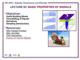
• Objectives:
Useful Building Blocks
Time-Shifting of Signals
Derivatives
Sampling (Introduction)
• Resources:
Wiki: Impulse Function
Wiki: Unit Step
TOH: Derivatives
Purdue: CT and DT Signals
LECTURE 02: BASIC PROPERTIES OF SIGNALS
Audio:
URL:

2. EE 3512: Lecture 02, Slide 2
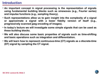
• An important concept in signal processing is the representation of signals
using fundamental building blocks such as sinewaves (e.g., Fourier series)
and impulse functions (e.g., sampling theory).
• Such representations allow us to gain insight into the complexity of a signal
or approximate a signal with a lower fidelity version of itself (e.g.,
progressively scanned jpeg encoding of images).
• In today’s lecture we will investigate some simple signals that can be used as
these building blocks.
• We will also discuss some basic properties of signals such as time-shifting
and basic operations such as integration and differentiation.
• We will learn how to represent continuous-time (CT) signals as a discrete-time
(DT) signal by sampling the CT signal.
Introduction

3. EE 3512: Lecture 02, Slide 3
The Impulse Function
• The unit impulse, also known as a Delta
function or a Dirac distribution, is defined by:
The impulse function can be approximated by a
rectangular pulse with amplitude A and time
duration 1/A.
• For any real number, K:
This is depicted to the right.
• The definition of an impulse for a DT signal is:
Note that:
 
  0
number
real
any
for
,
1
0
,
0
2
/
2
/













d
t
t
    0
for
,
2
/
2
/
2
/
2
/



 
 











K
d
K
d
K






0
,
0
0
,
1
]
[
n
n
n

  .
1





n
n

1/

K
t
t

4. EE 3512: Lecture 02, Slide 4
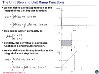
The Unit Step and Unit Ramp Functions
• We can define a unit step function as the
integral of the unit impulse function:
• This can be written compactly as:
• Similarly, the derivative of a unit step
function is a unit impulse function.
• We can define a unit ramp function as the
integral of a unit step function:
 
    0
for
,
1
0
for
,
0
)
(







 


 


t
d
d
t
d
t
u
t t
t
t









 
    0
for
,
0
for
,
0
)
(
0







 





t
t
d
u
d
u
t
d
u
t
r
t t
t






t
 






0
,
0
0
,
1
t
t
t
u

5. EE 3512: Lecture 02, Slide 5
The DT Unit Step and Unit Ramp Functions
• We can sum a DT unit pulse to arrive at a
DT unit step function:
• We can define a time-limited pulse, often referred
to as a discrete-time rectangular pulse:
• We can sum a unit step to arrive at
the unit ramp function:
 
      0
for
,
1
0
1
0
0
for
,
0
]
[
1










 


 


n
m
m
n
m
n
u
n
m
n
m
n
m




   
    0
for
,
0
for
,
0
0







 


 


n
n
m
m
u
n
m
u
n
r
n
m
n
m
n
m



 





n
other
all
,
0
2
/
)
1
(
,...,
1
,
0
,
1
,...,
2
/
)
1
(
,
1
]
[
L
L
n
n
pL

6. EE 3512: Lecture 02, Slide 6
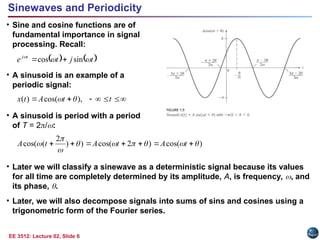
Sinewaves and Periodicity
• Sine and cosine functions are of
fundamental importance in signal
processing. Recall:
• A sinusoid is an example of a
periodic signal:
• A sinusoid is period with a period
of T = 2/:
• Later we will classify a sinewave as a deterministic signal because its values
for all time are completely determined by its amplitude, A, is frequency, , and
its phase, .
• Later, we will also decompose signals into sums of sins and cosines using a
trigonometric form of the Fourier series.
   
t
j
t
e t
j



sin
cos 







 t
t
A
t
x ),
cos(
)
( 

)
cos(
)
2
cos(
)
)
2
(
cos( 







 





 t
A
t
A
t
A

7. EE 3512: Lecture 02, Slide 7
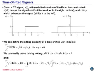
Time-Shifted Signals
• Given a CT signal, x(t), a time-shifted version of itself can be constructed:
x(t-t1) delays the signal (shifts it forward, or to the right, in time), and x(t+t1),
which advances the signal (shifts it to the left).
• We can define the sifting property of a time-shifted unit impulse:
We can easily prove this by noting:
and:
    0
any
for
),
(
1
1
1
1 












t
t
t
f
d
t
f
       
1
1
1 t
t
f
t
f 

 




           
  






























1
1
1
1
1
1
)
(
)
1
(
)
( 1
1
1
1
1
1
1
t
t
t
t
t
t
t
f
t
f
d
t
t
f
d
t
t
f
d
t
f

8. EE 3512: Lecture 02, Slide 8
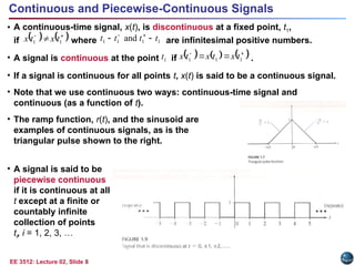
Continuous and Piecewise-Continuous Signals
• A continuous-time signal, x(t), is discontinuous at a fixed point, t1,
if where are infinitesimal positive numbers.
• A signal is continuous at the point if .
• If a signal is continuous for all points t, x(t) is said to be a continuous signal.
• Note that we use continuous two ways: continuous-time signal and
continuous (as a function of t).
• The ramp function, r(t), and the sinusoid are
examples of continuous signals, as is the
triangular pulse shown to the right.
• A signal is said to be
piecewise continuous
if it is continuous at all
t except at a finite or
countably infinite
collection of points
ti, i = 1, 2, 3, …
   


 1
1 t
x
t
x 1
1
1
1 and t
t
t
t 
 

1
t      



 1
1
1 t
x
t
x
t
x

9. EE 3512: Lecture 02, Slide 9
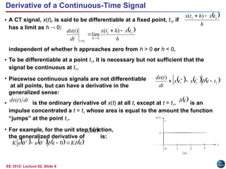
Derivative of a Continuous-Time Signal
• A CT signal, x(t), is said to be differentiable at a fixed point, t1, if
has a limit as h  0:
independent of whether h approaches zero from h > 0 or h < 0.
• To be differentiable at a point t1, it is necessary but not sufficient that the
signal be continuous at t1.
• Piecewise continuous signals are not differentiable
at all points, but can have a derivative in the
generalized sense:
• is the ordinary derivative of x(t) at all t, except at t = t1. is an
impulse concentrated a t = t1 whose area is equal to the amount the function
“jumps” at the point t1.
• For example, for the unit step function,
the generalized derivative of is:
 
h
t
x
h
t
x
dt
t
dx
h
t
t
1
1
0
)
(
lim
)
(
1





 
h
t
x
h
t
x 1
1 )
( 

   
   
1
1
1
)
(
t
t
t
x
t
x
dt
t
dx


 


dt
t
dx )
(  
t

 
t
Ku
   
     
t
K
t
u
u
K 
 

 

0
0
0

10. EE 3512: Lecture 02, Slide 10
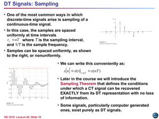
DT Signals: Sampling
• One of the most common ways in which
discrete-time signals arise is sampling of a
continuous-time signal.
• In this case, the samples are spaced
uniformly at time intervals
where T is the sampling interval,
and 1/T is the sample frequency.
• Samples can be spaced uniformly, as shown
to the right, or nonuniformly.
nT
tn 
• We can write this conveniently as:
• Later in the course we will introduce the
Sampling Theorem that defines the conditions
under which a CT signal can be recovered
EXACTLY from its DT representation with no loss
of information.
• Some signals, particularly computer generated
ones, exist purely as DT signals.
  )
(
)
( nT
x
t
x
n
x nT
t

 

11. EE 3512: Lecture 02, Slide 11
• Representation of signals using fundamental building blocks can be a useful
abstraction.
• We introduced four very important basic signals: impulse, unit step, ramp
and a sinewave. Further we introduced CT and DT versions of these.
• We introduced a mathematical representation for time-shifting a signal, and
introduced the sifting property.
• We discussed the concept of a continuous signal and noted that many of our
useful building blocks are discontinuous at some point in time (e.g., impulse
function). Further DT signals are inherently discontinuous.
• We introduced the concept of a derivative of a continuous signal and noted
that the derivative of a discrete-time signal is a bit more complicated.
• Finally, we presented some introductory material on sampling.
Summary