2
Local Searching
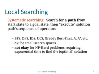
Systematic searching:Search for a path from
start state to a goal state, then “execute” solution
path’s sequence of operators
– BFS, DFS, IDS, UCS, Greedy Best-First, A, A*, etc.
– ok for small search spaces
– not okay for NP-Hard problems requiring
exponential time to find the (optimal) solution
AI - 4: Local Searching
5
Traveling Salesperson Problem(TSP)
A salesperson wants to visit a list of cities
stopping in each city only once
(sometimes also must return to the first city)
traveling the shortest distance
f = total distance traveled
AI - 4: Local Searching
6.
6
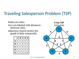
Traveling Salesperson Problem(TSP)
Nodes are cities
Arcs are labeled with distances
between cities
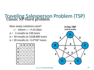
Adjacency matrix (notice the
graph is fully connected):
5 City TSP
(not to scale)
5
9
8
4
A
E
D
B C
5
6
7
5 3
2
A B C D E
A 0 5 8 9 7
B 5 0 6 5 5
C 8 6 0 2 3
D 9 5 2 0 4
E 7 5 3 4 0
AI - 4: Local Searching
7.
7
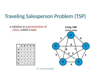
Traveling Salesperson Problem(TSP)
a solution is a permutation of
cities, called a tour
5 City TSP
(not to scale)
5
9
8
4
A
E
D
B C
5
6
7
5 3
2
A B C D E
A 0 5 8 9 7
B 5 0 6 5 5
C 8 6 0 2 3
D 9 5 2 0 4
E 7 5 3 4 0
AI - 4: Local Searching
8.
8
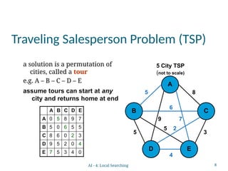
Traveling Salesperson Problem(TSP)
a solution is a permutation of
cities, called a tour
e.g. A – B – C – D – E
5 City TSP
(not to scale)
5
9
8
4
A
E
D
B C
5
6
7
5 3
2
A B C D E
A 0 5 8 9 7
B 5 0 6 5 5
C 8 6 0 2 3
D 9 5 2 0 4
E 7 5 3 4 0
assume tours can start at any
city and returns home at end
AI - 4: Local Searching
9.
9
How torepresent a state?
Successor function?
Heuristics?
How would you solve TSP
using A or A* Algorithm?
AI - 4: Local Searching
10.
10
Traveling Salesperson Problem(TSP)
How many solutions exist?
n! where n = # of cities
n = 5 results in 120 tours
n = 10 results in 3,628,800 tours
n = 20 results in ~2.4*1018
tours
5 City TSP
(not to scale)
5
9
8
4
A
E
D
B C
5
6
7
5 3
2
A B C D E
A 0 5 8 9 7
B 5 0 6 5 5
C 8 6 0 2 3
D 9 5 2 0 4
E 7 5 3 4 0
Classic NP-Hard problem
AI - 4: Local Searching
11.
11
Solving Optimization Problemsusing Local Search
Methods
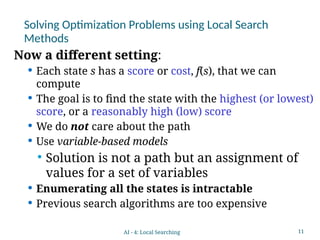
Now a different setting:
Each state s has a score or cost, f(s), that we can
compute
The goal is to find the state with the highest (or lowest)
score, or a reasonably high (low) score
We do not care about the path
Use variable-based models
Solution is not a path but an assignment of
values for a set of variables
Enumerating all the states is intractable
Previous search algorithms are too expensive
AI - 4: Local Searching
12.
12
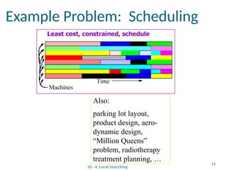
Example Problem: Scheduling
Also:
parkinglot layout,
product design, aero-
dynamic design,
“Million Queens”
problem, radiotherapy
treatment planning, …
AI - 4: Local Searching
13.
13
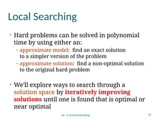
Local Searching
• Hardproblems can be solved in polynomial
time by using either an:
– approximate model: find an exact solution
to a simpler version of the problem
– approximate solution: find a non-optimal solution
to the original hard problem
• We'll explore ways to search through a
solution space by iteratively improving
solutions until one is found that is optimal or
near optimal
AI - 4: Local Searching
14.
14
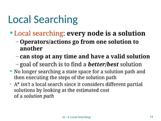
Local Searching
Localsearching: every node is a solution
– Operators/actions go from one solution to
another
– can stop at any time and have a valid solution
– goal of search is to find a better/best solution
No longer searching a state space for a solution path and
then executing the steps of the solution path
• A* isn't a local search since it considers different partial
solutions by looking at the estimated cost
of a solution path
AI - 4: Local Searching
15.
15
Local Searching
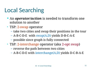
Anoperator/action is needed to transform one
solution to another
• TSP: 2-swap operator
– take two cities and swap their positions in the tour
– A-B-C-D-E with swap(A,D) yields D-B-C-A-E
– possible since graph is fully connected
• TSP: 2-interchange operator (aka 2-opt swap)
– reverse the path between two cities
– A-B-C-D-E with interchange(A,D) yields D-C-B-A-E
AI - 4: Local Searching
16.
16
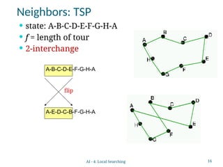
Neighbors: TSP
state:A-B-C-D-E-F-G-H-A
f = length of tour
2-interchange
A-B-C-D-E-F-G-H-A
A-E-D-C-B-F-G-H-A
flip
AI - 4: Local Searching
17.
17
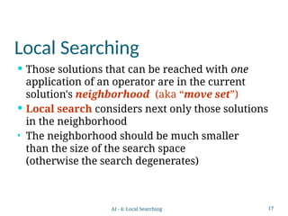
Local Searching
Thosesolutions that can be reached with one
application of an operator are in the current
solution's neighborhood (aka “move set”)
Local search considers next only those solutions
in the neighborhood
• The neighborhood should be much smaller
than the size of the search space
(otherwise the search degenerates)
AI - 4: Local Searching
18.
18
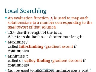
Local Searching
Anevaluation function, f, is used to map each
solution/state to a number corresponding to the
quality/cost of that solution
• TSP: Use the length of the tour;
A better solution has a shorter tour length
• Maximize f:
called hill-climbing (gradient ascent if
continuous)
• Minimize f:
called or valley-finding (gradient descent if
continuous)
• Can be used to maximize/minimize some cost
AI - 4: Local Searching
19.
19
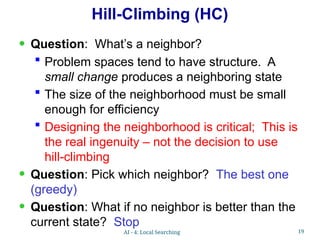
Hill-Climbing (HC)
• Question:What’s a neighbor?
Problem spaces tend to have structure. A
small change produces a neighboring state
The size of the neighborhood must be small
enough for efficiency
Designing the neighborhood is critical; This is
the real ingenuity – not the decision to use
hill-climbing
• Question: Pick which neighbor? The best one
(greedy)
• Question: What if no neighbor is better than the
current state? Stop
AI - 4: Local Searching
20.
20
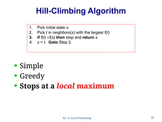
Hill-Climbing Algorithm
1. Pickinitial state s
2. Pick t in neighbors(s) with the largest f(t)
3. if f(t) <f(s) then stop and return s
4. s = t. Goto Step 2.
• Simple
• Greedy
• Stops at a local maximum
AI - 4: Local Searching
21.
21
Useful mentalpicture: f is a surface (‘hills’)
in state space
But we can’t see the entire landscape all at
once. Can only see a neighborhood; like
climbing in fog.
state
f
Global optimum,
where we want to be
Local Optima in Hill-Climbing
state
f
fog
AI - 4: Local Searching
22.
22
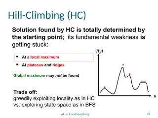
Hill-Climbing (HC)
Ata local maximum
At plateaus and ridges
Global maximum may not be found
f(y)
y
Trade off:
greedily exploiting locality as in HC
vs. exploring state space as in BFS
Solution found by HC is totally determined by
the starting point; its fundamental weakness is
getting stuck:
AI - 4: Local Searching
23.
23
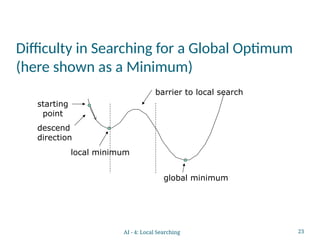
Difficulty in Searchingfor a Global Optimum
(here shown as a Minimum)
starting
point
descend
direction
local minimum
global minimum
barrier to local search
AI - 4: Local Searching
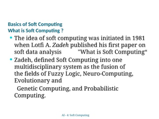
Basics of SoftComputing
What is Soft Computing ?
The idea of soft computing was initiated in 1981
when Lotfi A. Zadeh published his first paper on
soft data analysis "What is Soft Computing“
Zadeh, defined Soft Computing into one
multidisciplinary system as the fusion of
the fields of Fuzzy Logic, Neuro-Computing,
Evolutionary and
Genetic Computing, and Probabilistic
Computing.
AI - 4: Soft Computing
28.
• Soft Computingis the fusion of methodologies
designed to model and enable solutions to real
world problems, which are not modeled or too
difficult to model mathematically.
• The aim of Soft Computing is to exploit the
tolerance for imprecision, uncertainty,
approximate reasoning, and partial truth in
order to achieve close resemblance with human
like decision making.
AI - 4: Soft Computing
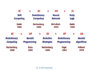
Definitions of SoftComputing (SC)
Lotfi A. Zadeh, 1 99 2 :
"Soft Computing is an emerging approach
to computing which parallel the remarkable
ability of the human mind to reason and learn in
a environment of uncertainty and imprecision"
AI - 4: Soft Computing
31.
The Soft Computingconsists of several
computing paradigms mainly :
Fuzzy Systems, Neural Networks, and Genetic
Algorithms.
• Fuzzy set : for knowledge representation via fuzzy
If - Then rules.
• Neural Networks : for learning and adaptation
• Genetic Algorithms : for evolutionary computation
AI - 4: Soft Computing
32.
These methodologiesform the core of SC.
Hybridization of these three creates a successful
synergic effect; that is, hybridization creates a
situation where different entities cooperate
advantageously for a final outcome.
Soft Computing is still growing and developing.
Hence, a clear definite agreement on what
comprises Soft Computing has not yet been
reached. More new sciences are still merging
into Soft Computing.
AI - 4: Soft Computing
33.
Goals of SoftComputing
Soft Computing is a new multidisciplinary field,
to construct new generation of Artificial
Intelligence, known as Computational
Intelligence.
The main goal of Soft Computing is to develop
intelligent machines to provide solutions to real
world problems, which are not modeled, or too
difficult to model mathematically.
AI - 4: Soft Computing
34.
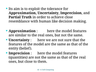
Its aimis to exploit the tolerance for
Approximation, Uncertainty, Imprecision, and
Partial Truth in order to achieve close
resemblance with human like decision making.
Approximation : here the model features
are similar to the real ones, but not the same.
Uncertainty : here we are not sure that the
features of the model are the same as that of the
entity (belief).
Imprecision : here the model features
(quantities) are not the same as that of the real
ones, but close to them.
AI - 4: Soft Computing
35.
Applications
The applications ofSoft Computing have proved
two the advantages:
First, in solving nonlinear problems; where
mathematical models are not available or not
possible.
Second, introducing the human knowledge such
as cognition, recognition, understanding,
learning, and others into the field of computing.
AI - 4: Soft Computing
36.
The resultedin the possibility of constructing
intelligent systems such as autonomous self-
tuning systems, and automated design system
AI - 4: Soft Computing
37.
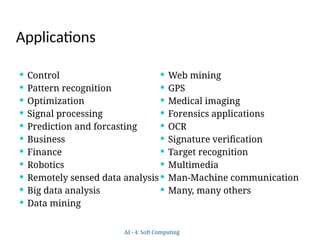
Applications
Control
Patternrecognition
Optimization
Signal processing
Prediction and forcasting
Business
Finance
Robotics
Remotely sensed data analysis
Big data analysis
Data mining
Web mining
GPS
Medical imaging
Forensics applications
OCR
Signature verification
Target recognition
Multimedia
Man-Machine communication
Many, many others
AI - 4: Soft Computing
38.
38
Syllabus
To begin,first explained,
the definitions,
the goals, and
the importance of the soft computing.
Later, presented its different fields, that is,
Neural Computing
Evolutionary Computing
Fuzzy Computing
AI - 4: Soft Computing
#22 CLICK ANIM: 1. solution text, 2. diagram, 3. local max text, 4. local max points, 5. plateau text, 6. plateau line,
7. global max text, 8. global max point, 9. trade off text
explain how start determines solution
HC starting is Madison would get stuck on Bascom hill
#23 Local search techniques, such as steepest descend method, are very good in finding local optima. However, difficulties arise when the global optima is different from the local optima. Since all the immediate neighboring points around a local optima is worse than it in the performance value, local search can not proceed once trapped in a local optima point. We need some mechanism that can help us escape the trap of local optima. And the simulated annealing is one of such methods.


![tilt sensor Mundher Al_tiabi.pptx [تم الإصلاح]_33٠٢٢١٣٤_٠٧١٦٤٨.pptx](https://cdn.slidesharecdn.com/ss_thumbnails/tiltsensormundheraltiabi-251106125741-7aadf2db-thumbnail.jpg?width=640&height=640&fit=bounds)


