Story so far
•Pattern classification tasks such as “does this picture contain a cat”, or
“does this recording include HELLO” are best performed by scanning for
the target pattern
• Scanning an input with a network and combining the outcomes is
equivalent to scanning with individual neurons hierarchically
– First level neurons scan the input
– Higher-level neurons scan the “maps” formed by lower-level neurons
– A final “decision” unit or subnetwork makes the final decision
• Deformations in the input can be handled by “pooling”
• For 2-D (or higher-dimensional) scans, the structure is called a
convolutional network
• For 1-D scan along time, it is called a Time-delay neural network
2
A little history
•How do animals see?
– What is the neural process from eye to recognition?
• Early research:
– largely based on behavioral studies
• Study behavioral judgment in response to visual stimulation
• Visual illusions
– and gestalt
• Brain has innate tendency to organize disconnected bits into whole objects
– But no real understanding of how the brain processed images
4
5.
Hubel and Wiesel1959
• First study on neural correlates of vision.
– “Receptive Fields in Cat Striate Cortex”
• “Striate Cortex”: Approximately equal to the V1 visual cortex
– “Striate” – defined by structure, “V1” – functional definition
• 24 cats, anaesthetized, immobilized, on artificial respirators
– Anaesthetized with truth serum
– Electrodes into brain
• Do not report if cats survived experiment, but claim brain tissue was studied
5
6.
Hubel and Wiesel1959
• Light of different wavelengths incident on the retina
through fully open (slitted) Iris
– Defines immediate (20ms) response of retinal cells
• Beamed light of different patterns into the eyes and
measured neural responses in striate cortex
6
7.
Hubel and Wiesel1959
• Restricted retinal areas which on illumination influenced the firing of single cortical
units were called receptive fields.
– These fields were usually subdivided into excitatory and inhibitory regions.
• Findings:
– A light stimulus covering the whole receptive field, or diffuse illumination of the whole retina,
was ineffective in driving most units, as excitatory regions cancelled inhibitory regions
• Light must fall on excitatory regions and NOT fall on inhibitory regions, resulting in clear patterns
– A spot of light gave greater response for some directions of movement than others.
• Can be used to determine the receptive field
– Receptive fields could be oriented in a vertical, horizontal or oblique manner.
• Based on the arrangement of excitatory and inhibitory regions within receptive fields.
mice
monkey
From Huberman and Neil, 2011
From Hubel and Wiesel
7
8.
Hubel and Wiesel59
• Response as orientation of input light rotates
– Note spikes – this neuron is sensitive to vertical bands
8
9.
Hubel and Wiesel
•Oriented slits of light were the most effective stimuli for activating
striate cortex neurons
• The orientation selectivity resulted from the previous level of input
because lower-level neurons responding to a slit also responded to
patterns of spots if they were aligned with the same orientation as
the slit.
• In a later paper (Hubel & Wiesel, 1962), they showed that within
the striate cortex, two levels of processing could be identified
– Between neurons referred to as simple S-cells and complex C-cells.
– Both types responded to oriented slits of light, but complex cells were
not “confused” by spots of light while simple cells could be confused
9
10.
Hubel and Wieselmodel
• ll
Transform from circular retinal
receptive fields to elongated fields for
simple cells. The simple cells are
susceptible to fuzziness and noise
Composition of complex receptive
fields from simple cells. The C-cell
responds to the largest output from a
bank of S-cells to achieve oriented
response that is robust to distortion
10
11.
Hubel and Wiesel
•Complex C-cells build from similarly oriented simple cells
– They “fine-tune” the response of the simple cell
• Show complex buildup – building more complex patterns
by composing early neural responses
– Successive transformation through Simple-Complex
combination layers
• Demonstrated more and more complex responses in
later papers
– Later experiments were on waking macaque monkeys
• Too horrible to recall
11
12.
Hubel and Wiesel
•Complex cells build from similarly oriented simple cells
– The “tune” the response of the simple cell and have similar response to the simple cell
• Show complex buildup – from point response of retina to oriented response of
simple cells to cleaner response of complex cells
• Lead to more complex model of building more complex patterns by composing
early neural responses
– Successive transformations through Simple-Complex combination layers
• Demonstrated more and more complex responses in later papers
• Experiments done by others were on waking monkeys
– Too horrible to recall
12
13.
Adding insult toinjury..
• “However, this model cannot accommodate
the color, spatial frequency and many other
features to which neurons are tuned. The
exact organization of all these cortical columns
within V1 remains a hot topic of current
research.”
13
Poll 1
15
According toHubel and Wiesel which type of cells found patterns in the input and which cells “cleaned”
up these patterns?
S cells find patterns and C cells clean them up
C cells find patterns and S cells clean them up
16.
Forward to 1980
•Kunihiko Fukushima
• Recognized deficiencies in the
Hubel-Wiesel model
• One of the chief problems: Position invariance of
input
– Your grandmother cell fires even if your grandmother
moves to a different location in your field of vision
Kunihiko Fukushima
16
17.
NeoCognitron
• Visual systemconsists of a hierarchy of modules, each comprising a
layer of “S-cells” followed by a layer of “C-cells”
– is the lth layer of S cells, is the lth layer of C cells
• S-cells respond to the signal in the previous layer
• C-cells confirm the S-cells’ response
• Only S-cells are “plastic” (i.e. learnable), C-cells are fixed in their
response
Figures from Fukushima, ‘80
17
18.
NeoCognitron
• Each simple-complexmodule includes a layer of S-cells and a layer of C-cells
• S-cells are organized in rectangular groups called S-planes.
– All the cells within an S-plane have identical learned responses
• C-cells too are organized into rectangular groups called C-planes
– One C-plane per S-plane
– All C-cells have identical fixed response
• In Fukushima’s original work, each C and S cell “looks” at an elliptical region in the
previous plane
Each cell in a plane “looks” at a slightly shifted
region of the input than the adjacent cells in
the plane.
… “through” the previous layer planes
18
19.
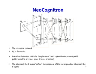
NeoCognitron
• The completenetwork
• U0 is the retina
• In each subsequent module, the planes of the S layers detect plane-specific
patterns in the previous layer (C layer or retina)
• The planes of the C layers “refine” the response of the corresponding planes of the
S layers 19
20.
Neocognitron
• S cells:RELU like activation
– is a RELU
• C cells: Also RELU like, but with an inhibitory bias
– Fires if weighted combination of S cells fires strongly
enough
–
20
21.
Neocognitron
• S cells:RELU like activation
– is a RELU
• C cells: Also RELU like, but with an inhibitory bias
– Fires if weighted combination of S cells fires strongly
enough
–
Could simply replace these
strange functions with a
RELU and a max
21
22.
NeoCognitron
• The deeperthe layer, the larger the receptive field of
each neuron
– Cell planes get smaller with layer number
– Number of planes increases
• i.e the number of complex pattern detectors increases with layer 22
23.
Learning in theneocognitron
• Unsupervised learning
• Randomly initialize S cells, perform Hebbian learning updates in response to input
– update = product of input and output : ∆𝑤 = 𝑥 𝑦
• Within any layer, at any position, only the maximum S from all the layers is
selected for update
– Also viewed as max-valued cell from each S column
• Ensures only one of the planes picks up any feature
• If multiple max selections are on the same plane, only the largest is chosen
– But across all positions, multiple planes will be selected
• Updates are distributed across all cells within the plane
max
23
24.
Learning in theneocognitron
• Ensures different planes learn different features
– E.g. Given many examples of the character “A” the different cell
planes in the S-C layers may learn the patterns shown
• Given other characters, other planes will learn their components
– Going up the layers goes from local to global receptor fields
• Winner-take-all strategy makes it robust to distortion
• Unsupervised: Effectively clustering
24
25.
Neocognitron – finale
•Fukushima showed it successfully learns to
cluster semantic visual concepts
– E.g. number or characters, even in noise
25
Poll 2
27
Fukushima’s modelis an unsupervised CNN, true or false
True
False
Supervision can be added to Fukushima’s model, true or false
True
False
28.
Adding Supervision
• Theneocognitron is fully unsupervised
– Semantic labels are automatically learned
• Can we add external supervision?
• Various proposals:
– Temporal correlation: Homma, Atlas, Marks, ‘88
– TDNN: Lang, Waibel et. al., 1989, ‘90
• Convolutional neural networks: LeCun
28
29.
Supervising the neocognitron
•Add an extra decision layer after the final C layer
– Produces a class-label output
• We now have a fully feed forward MLP with shared parameters
– All the S-cells within an S-plane have the same weights
• Simple backpropagation can now train the S-cell weights in every plane of
every layer
– C-cells are not updated
Output
class
label(s)
29
30.
Scanning vs. multiplefilters
• Note: The original Neocognitron actually uses many
identical copies of a neuron in each S and C plane
– Mathematically identical to “scanning” with a single copy
30
31.
Supervising the neocognitron
•The Math
– Assuming square receptive fields, rather than elliptical ones
– Receptive field of S cells in lth layer is
– Receptive field of C cells in lth layer is
• C cells “stride” by more than one pixel, resulting in a shrinking, or “downsampling” of
the maps
Output
class
label(s)
31
32.
Supervising the neocognitron
•This is, identical to “scanning” (convolving) with a
single neuron/filter (what LeNet actually did)
Output
class
label(s)
𝑺,𝒍,𝒏 𝑺,𝒍,𝒏 𝑪,𝒍 𝟏,𝒑
𝑲𝒍
𝑲𝒍
𝒑
𝑪,𝒍,𝒏
∈ , , ∈( , )
𝑺,𝒍,𝒏
32
Story so far
•The mammalian visual cortex contains of S cells, which capture oriented
visual patterns and C cells which perform a “majority” vote over groups of
S cells for robustness to noise and positional jitter
• The neocognitron emulates this behavior with planar banks of S and C
cells with identical response, to enable shift invariance
– Only S cells are learned
– C cells perform the equivalent of a max over groups of S cells for robustness
– Unsupervised learning results in learning useful patterns
• LeCun’s LeNet added external supervision to the neocognitron
– S planes of cells with identical response are modelled by a scan (convolution)
over image planes by a single neuron
– C planes are emulated by cells that perform a max over groups of S cells
• Reducing the size of the S planes
– Giving us a “Convolutional Neural Network” 34
35.
The general architectureof a
convolutional neural network
• A convolutional neural network comprises “convolutional” and “downsampling” layers
– Convolutional layers comprise neurons that scan their input for patterns
• Correspond to S planes
– Downsampling layers perform max operations on groups of outputs from the convolutional layers
• Correspond to C planes
– The two may occur in any sequence, but typically they alternate
• Followed by an MLP with one or more layers
Multi-layer
Perceptron
Output
35
36.
The general architectureof a
convolutional neural network
• A convolutional neural network comprises of “convolutional” and
“downsampling” layers
– The two may occur in any sequence, but typically they alternate
• Followed by an MLP with one or more layers
Multi-layer
Perceptron
Output
36
37.
The general architectureof a
convolutional neural network
• Convolutional layers and the MLP are learnable
– Their parameters must be learned from training data for the target
classification task
• Down-sampling layers are fixed and generally not learnable
Multi-layer
Perceptron
Output
37
38.
A convolutional layer
•A convolutional layer comprises of a series of “maps”
– Corresponding the “S-planes” in the Neocognitron
– Variously called feature maps or activation maps
Maps
Previous
layer
38
39.
A convolutional layer
•Each activation map has two components
– An affine map, obtained by convolution over maps in the previous layer
• Each affine map has, associated with it, a learnable filter
– An activation that operates on the output of the convolution
Previous
layer
Previous
layer
39
40.
A convolutional layer:affine map
• All the maps in the previous layer contribute
to each convolution
Previous
layer
Previous
layer
40
41.
A convolutional layer:affine map
• All the maps in the previous layer contribute to
each convolution
– Consider the contribution of a single map
Previous
layer
Previous
layer
41
42.
What is aconvolution
• Scanning an image with a “filter”
– Note: a filter is really just a perceptron, with weights
and a bias
1 1 1 0 0
0 1 1 1 0
1 1 1
0 0
0 0 0
1 1
0 1 0
1 0
Example 5x5 image with binary
pixels
1 0 1
0 1 0
1
1 0
0
Example 3x3 filter
bias
42
43.
What is aconvolution
• Scanning an image with a “filter”
– At each location, the “filter and the underlying map values are
multiplied component wise, and the products are added along with
the bias
1 0 1
0 1 0
1
1 0
Input Map
Filter
0
bias
43
44.
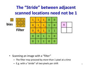
The “Stride” betweenadjacent
scanned locations need not be 1
• Scanning an image with a “filter”
– The filter may proceed by more than 1 pixel at a time
– E.g. with a “stride” of two pixels per shift
1 1 1 0 0
0 1 1 1 0
1 1 1
0 0
0 0 0
1 1
0 1 0
1 0
4
x1 x0 x1
x0 x1 x0
x1
x1 x0
1 0 1
0 1 0
1
1 0
Filter
0
bias
44
45.
The “Stride” betweenadjacent
scanned locations need not be 1
• Scanning an image with a “filter”
– The filter may proceed by more than 1 pixel at a time
– E.g. with a “hop” of two pixels per shift
1 1 1 0 0
0 1 1 1 0
1 1 1
0 0
0 0 0
1 1
0 1 0
1 0
x1 x0 x1
x0 x1 x0
x1
x1 x0
1 0 1
0 1 0
1
1 0
Filter
0
bias 4 4
45
46.
The “Stride” betweenadjacent
scanned locations need not be 1
• Scanning an image with a “filter”
– The filter may proceed by more than 1 pixel at a time
– E.g. with a “hop” of two pixels per shift
1 1 1 0 0
0 1 1 1 0
1 1 1
0 0
0 0 0
1 1
0 1 0
1 0
x1 x0 x1
x0 x1 x0
x1
x1 x0
1 0 1
0 1 0
1
1 0
Filter
0
bias 4 4
2
46
47.
The “Stride” betweenadjacent
scanned locations need not be 1
• Scanning an image with a “filter”
– The filter may proceed by more than 1 pixel at a time
– E.g. with a “hop” of two pixels per shift
1 1 1 0 0
0 1 1 1 0
1 1 1
0 0
0 0 0
1 1
0 1 0
1 0
x1 x0 x1
x0 x1 x0
x1
x1 x0
1 0 1
0 1 0
1
1 0
Filter
0
bias 4 4
2 4
47
48.
What really happens
•Each output is computed from multiple maps simultaneously
• There are as many weights (for each output map) as
size of the filter x no. of maps in previous layer
Previous
layer
filter
Input layer
Output map
48
49.
What really happens
•Each output is computed from multiple maps simultaneously
• There are as many weights (for each output map) as
size of the filter x no. of maps in previous layer
𝑧 1,𝑖, 𝑗 = 𝑤 1,𝑚, 𝑘, 𝑙 𝐼 𝑚, 𝑖 + 𝑙 − 1, 𝑗 + 𝑘 − 1 + 𝑏
Previous
layer
Input layer
Output map
49
50.
What really happens
•Each output is computed from multiple maps simultaneously
• There are as many weights (for each output map) as
size of the filter x no. of maps in previous layer
𝑧 1,𝑖, 𝑗 = 𝑤 1,𝑚, 𝑘, 𝑙 𝐼 𝑚, 𝑖 + 𝑙 − 1, 𝑗 + 𝑘 − 1 + 𝑏
Previous
layer
Input layer
Output map
50
51.
What really happens
•Each output is computed from multiple maps simultaneously
• There are as many weights (for each output map) as
size of the filter x no. of maps in previous layer
Previous
layer
𝑧 1,𝑖, 𝑗 = 𝑤 1,𝑚, 𝑘, 𝑙 𝐼 𝑚, 𝑖 + 𝑙 − 1, 𝑗 + 𝑘 − 1 + 𝑏
Input layer
Output map
51
52.
What really happens
•Each output is computed from multiple maps simultaneously
• There are as many weights (for each output map) as
size of the filter x no. of maps in previous layer
Previous
layer
𝑧 1,𝑖, 𝑗 = 𝑤 1,𝑚, 𝑘, 𝑙 𝐼 𝑚, 𝑖 + 𝑙 − 1, 𝑗 + 𝑘 − 1 + 𝑏
Input layer
Output map
52
53.
What really happens
•Each output is computed from multiple maps simultaneously
• There are as many weights (for each output map) as
size of the filter x no. of maps in previous layer
Previous
layer
𝑧 1,𝑖, 𝑗 = 𝑤 1,𝑚, 𝑘, 𝑙 𝐼 𝑚, 𝑖 + 𝑙 − 1, 𝑗 + 𝑘 − 1 + 𝑏
Input layer
Output map
53
54.
What really happens
•Each output is computed from multiple maps simultaneously
• There are as many weights (for each output map) as
size of the filter x no. of maps in previous layer
Previous
layer
𝑧 1,𝑖, 𝑗 = 𝑤 1,𝑚, 𝑘, 𝑙 𝐼 𝑚, 𝑖 + 𝑙 − 1, 𝑗 + 𝑘 − 1 + 𝑏
Input layer
Output map
54
55.
What really happens
•Each output is computed from multiple maps simultaneously
• There are as many weights (for each output map) as
size of the filter x no. of maps in previous layer
𝑧 1,𝑖, 𝑗 = 𝑤 1,𝑚, 𝑘, 𝑙 𝐼 𝑚, 𝑖 + 𝑙 − 1, 𝑗 + 𝑘 − 1 + 𝑏
Previous
layer
Input layer
Output map
55
56.
What really happens
•Each output is computed from multiple maps simultaneously
• There are as many weights (for each output map) as
size of the filter x no. of maps in previous layer
Previous
layer
𝑧 1,𝑖, 𝑗 = 𝑤 1,𝑚, 𝑘, 𝑙 𝐼 𝑚, 𝑖 + 𝑙 − 1, 𝑗 + 𝑘 − 1 + 𝑏
Input layer
Output map
56
57.
What really happens
•Each output is computed from multiple maps simultaneously
• There are as many weights (for each output map) as
size of the filter x no. of maps in previous layer
Previous
layer
𝑧 1,𝑖, 𝑗 = 𝑤 1,𝑚, 𝑘, 𝑙 𝐼 𝑚, 𝑖 + 𝑙 − 1, 𝑗 + 𝑘 − 1 + 𝑏
Input layer
Output map
57
58.
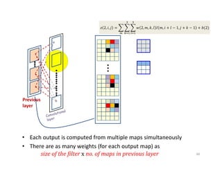
• Each outputis computed from multiple maps simultaneously
• There are as many weights (for each output map) as
size of the filter x no. of maps in previous layer
𝑧 2,𝑖, 𝑗 = 𝑤 2,𝑚, 𝑘, 𝑙 𝐼 𝑚, 𝑖 + 𝑙 − 1, 𝑗 + 𝑘 − 1 + 𝑏(2)
Previous
layer
filter1 filter2
58
59.
• Each outputis computed from multiple maps simultaneously
• There are as many weights (for each output map) as
size of the filter x no. of maps in previous layer
Previous
layer
𝑧 2,𝑖, 𝑗 = 𝑤 2,𝑚, 𝑘, 𝑙 𝐼 𝑚, 𝑖 + 𝑙 − 1, 𝑗 + 𝑘 − 1 + 𝑏(2)
59
60.
• Each outputis computed from multiple maps simultaneously
• There are as many weights (for each output map) as
size of the filter x no. of maps in previous layer
Previous
layer
𝑧 2,𝑖, 𝑗 = 𝑤 2,𝑚, 𝑘, 𝑙 𝐼 𝑚, 𝑖 + 𝑙 − 1, 𝑗 + 𝑘 − 1 + 𝑏(2)
60
61.
A different view
•..A stacked arrangement of planes
• We can view the joint processing of the various
maps as processing the stack using a three-
dimensional filter
Stacked arrangement
of kth layer of maps
Filter applied to kth layer of maps
(convolutive component plus bias)
61
62.
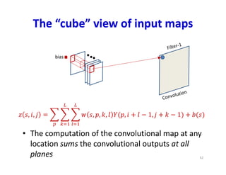
The “cube” viewof input maps
• The computation of the convolutional map at any
location sums the convolutional outputs at all
planes
bias
62
63.
• The computationof the convolutional map at any
location sums the convolutional outputs at all
planes
One map
bias
The “cube” view of input maps
63
64.
• The computationof the convolutional map at any
location sums the convolutional outputs at all
planes
All maps
bias
The “cube” view of input maps
64
65.
• The computationof the convolutional map at any
location sums the convolutional outputs at all
planes
bias
The “cube” view of input maps
65
66.
• The computationof the convolutional map at any
location sums the convolutional outputs at all
planes
bias
The “cube” view of input maps
66
67.
• The computationof the convolutional map at any
location sums the convolutional outputs at all
planes
bias
The “cube” view of input maps
67
68.
• The computationof the convolutional map at any
location sums the convolutional outputs at all
planes
bias
The “cube” view of input maps
68
69.
• The computationof the convolutional map at any
location sums the convolutional outputs at all
planes
bias
The “cube” view of input maps
69
70.
CNN: Vector notationto compute a
single output map
The weight W(l,j)is now a 3D Dl-1xKlxKl tensor (assuming
square receptive fields)
The product in blue is a tensor inner product with a
scalar output
Y(0) = Image
for l = 1:L # layers operate on vector at (x,y)
for x = 1:Wl-1-Kl+1
for y = 1:Hl-1-Kl+1
for j = 1:Dl
segment = Y(l-1,:,x:x+Kl-1,y:y+Kl-1) #3D tensor
z(l,j,x,y) = W(l,j).segment #tensor inner prod.
Y(l,j,x,y) = activation(z(l,j,x,y))
Y = softmax( {Y(L,:,:,:)} )
70
71.
Engineering consideration: Thesize of
the result of the convolution
• The size of the output of the convolution operation depends on
implementation factors
– The size of the input, the size of the filter, and the stride
• And may not be identical to the size of the input
– Let’s take a brief look at this for completeness sake
bias
71
The size ofthe convolution
• Image size:
• Filter:
• Stride:
• Output size (each side) =
– Assuming you’re not allowed to go beyond the edge of the input
1 1 1 0 0
0 1 1 1 0
1 1 1
0 0
0 0 0
1 1
0 1 0
1 0
Filter
0
bias
?
78
79.
Convolution Size
• Simpleconvolution size pattern:
– Image size:
– Filter:
– Stride:
– Output size (each side) =
• Assuming you’re not allowed to go beyond the edge of the input
• Results in a reduction in the output size
– Even if
– Sometimes not considered acceptable
• If there’s no active downsampling, through max pooling and/or
, then the output map should ideally be the same size as the
input
79
80.
Solution
• Zero-pad theinput
– Pad the input image/map all around
• Add PL rows of zeros on the left and PR rows of zeros on the right
• Add PL rows of zeros on the top and PL rows of zeros at the bottom
– PL and PR chosen such that:
• PL = PR OR | PL – PR| = 1
• PL+ PR = M-1
– For stride 1, the result of the convolution is the same size as the original
image
1 1 1 0 0
0 1 1 1 0
1 1 1
0 0
0 0 0
1 1
0 1 0
1 0
1 0 1
0 1 0
1
1 0
Filter
0
bias
0
0
0
0
0
0
0
0
0
0
0 0 0 0 0
0 0
0 0 0 0 0
0 0
80
81.
Solution
• Zero-pad theinput
– Pad the input image/map all around
– Pad as symmetrically as possible, such that..
– For stride 1, the result of the convolution is the
same size as the original image
1 1 1 0 0
0 1 1 1 0
1 1 1
0 0
0 0 0
1 1
0 1 0
1 0
1 0 1
0 1 0
1
1 0
Filter
0
bias
0
0
0
0
0
0
0
0
0
0
0 0 0 0 0
0 0
0 0 0 0 0
0 0
81
82.
Zero padding
• Foran width filter:
– Odd : Pad on both left and right with columns of zeros
– Even : Pad one side with columns of zeros, and the other with
columns of zeros
– The resulting image is width
– The result of the convolution is width
• The top/bottom zero padding follows the same rules to maintain
map height after convolution
• For hop size , zero padding is adjusted to ensure that the size
of the convolved output is
– Achieved by first zero padding the image with
columns/rows of zeros and then applying above rules
82
83.
A convolutional layer
•The convolution operation results in an affine map
• An Activation is finally applied to every entry in the map
Previous
layer
Previous
layer
83
84.
Convolutional neural net:
Vectornotation
The weight W(l,j)is now a 4D DlxDl-1xKlxKl tensor (assuming
square receptive fields)
The product in blue is a tensor inner product with a
scalar output
Y(0) = Image
for l = 1:L # layers operate on vector at (x,y)
for x = 1:Wl-1-Kl+1
for y = 1:Hl-1-Kl+1
segment = Y(l-1,:,x:x+Kl-1,y:y+Kl-1) #3D tensor
z(l,:,x,y) = W(l).segment #tensor inner prod.
Y(l,:,x,y) = activation(z(l,;,x,y))
Y = softmax( {Y(L,:,:,:)} )
84
85.
The other component
Downsampling/Pooling
•Convolution (and activation) layers are followed intermittently by
“downsampling with pooling” layers
– Typically (but not always) “max” pooling
– Often, they alternate with convolution, though this is not necessary
Multi-layer
Perceptron
Output
85
86.
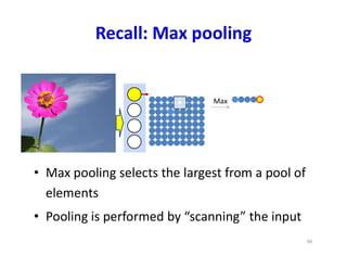
Max pooling
• Maxpooling selects the largest from a pool of
elements
• Pooling is performed by “scanning” the input
Max
3 1
4 6
Max
6
86
87.
Recall: Max pooling
Max
13
6 5
Max
6 6
• Max pooling selects the largest from a pool of
elements
• Pooling is performed by “scanning” the input
87
88.
Recall: Max pooling
Max
32
5 7
Max
6 6 7
• Max pooling selects the largest from a pool of
elements
• Pooling is performed by “scanning” the input
88
89.
Recall: Max pooling
Max
•Max pooling selects the largest from a pool of
elements
• Pooling is performed by “scanning” the input
89
90.
Recall: Max pooling
Max
•Max pooling selects the largest from a pool of
elements
• Pooling is performed by “scanning” the input
90
91.
Recall: Max pooling
Max
•Max pooling scans with a stride of 1 confer
jitter-robustness, but do not constitute
downsampling
• Downsampling requires a stride greater than 1
91
92.
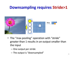
Downsampling requires Stride>1
•The “max pooling” operation with “stride”
greater than 1 results in an output smaller than
the input
– One output per stride
– The output is “downsampled”
Max
92
93.
• The “maxpooling” operation with “stride”
greater than 1 results in an output smaller than
the input
– One output per stride
– The output is “downsampled”
Max
Downsampling requires Stride>1
93
94.
• The “maxpooling” operation with “stride”
greater than 1 results in an output smaller than
the input
– One output per stride
– The output is “downsampled”
Max
Downsampling requires Stride>1
94
95.
• The “maxpooling” operation with “stride”
greater than 1 results in an output smaller than
the input
– One output per stride
– The output is “downsampled”
Max
Downsampling requires Stride>1
95
96.
• The “maxpooling” operation with “stride”
greater than 1 results in an output smaller than
the input
– One output per stride
– The output is “downsampled”
Max
Downsampling requires Stride>1
96
97.
• The “maxpooling” operation with “stride”
greater than 1 results in an output smaller than
the input
– One output per stride
– The output is “downsampled”
Max
Downsampling requires Stride>1
97
98.
• The “maxpooling” operation with “stride”
greater than 1 results in an output smaller than
the input
– One output per stride
– The output is “downsampled”
Max
Downsampling requires Stride>1
98
99.
• The “maxpooling” operation with “stride”
greater than 1 results in an output smaller than
the input
– One output per stride
– The output is “downsampled”
Max
Downsampling requires Stride>1
99
100.
• The “maxpooling” operation with “stride”
greater than 1 results in an output smaller than
the input
– One output per stride
– The output is “downsampled”
Downsampling requires Stride>1
Max
100
101.
Max Pooling layerat layer
Max pooling
for j = 1:Dl
m = 1
for x = 1:stride(l):Wl-1-Kl+1
n = 1
for y = 1:stride(l):Hl-1-Kl+1
pidx(l,j,m,n) = maxidx(Y(l-1,j,x:x+Kl-1,y:y+Kl-1))
Y(l,j,m,n) = Y(l-1,j,pidx(l,j,m,n))
n = n+1
m = m+1
101
a) Performed separately for every map (j).
*) Not combining multiple maps within a single max operation.
b) Keeping track of location of max
102.
1 1 24
5 6 7 8
3 2 1 0
1 2 3 4
Single depth slice
x
y
max pool with 2x2 filters
and stride 2 6 8
3 4
Downsampling: Size of output
• An picture compressed by a pooling filter with
stride results in an output map of side
• Typically do not zero pad
103.
1 1 24
5 6 7 8
3 2 1 0
1 2 3 4
Single depth slice
x
y
Mean pool with 2x2
filters and stride 2 3.25 5.25
2 2
Alternative to Max pooling:
Mean Pooling
• Compute the mean of the pool, instead of the max
104.
Mean Pooling layerat layer
Mean pooling
for j = 1:Dl
m = 1
for x = 1:stride(l):Wl-1-Kl+1
n = 1
for y = 1:stride(l):Hl-1-Kl+1
Y(l,j,m,n) = mean(Y(l-1,j,x:x+Kl-1,y:y+Kl-1))
n = n+1
m = m+1
104
a) Performed separately for every map (j)
105.
Alternative to Maxpooling:
-norm
• Compute a p-norm of the pool
1 1 2 4
5 6 7 8
3 2 1 0
1 2 3 4
Single depth slice
x
y
P-norm with 2x2 filters
and stride 2, = 5 4.86 8
2.38 3.16
,
106.
Other options
• Thepooling may even be a learned filter
• The same network is applied on each block
• (Again, a shared parameter network)
1 1 2 4
5 6 7 8
3 2 1 0
1 2 3 4
Single depth slice
x
y
Network applies to each
2x2 block and strides by
2 in this example
6 8
3 4
Network in network
107.
Or even onlywith conovlutions
• Downsampling may even be done by a simple convolution
layer with stride larger than 1
– Replacing the maxpooling layer with a conv layer
Just a plain old convolution
layer with stride>1
107
108.
Fully convolutional network
(nopooling)
The weight W(l,j)is now a 3D Dl-1xKlxKl tensor (assuming
square receptive fields)
The product in blue is a tensor inner product with a
scalar output
Y(0) = Image
for l = 1:L # layers operate on vector at (x,y)
for x,m = 1:stride(l):Wl-1-Kl+1 # double indices
for y,n = 1:stride(l):Hl-1-Kl+1
for j = 1:Dl
segment = y(l-1,:,x:x+Kl-1,y:y+Kl-1) #3D tensor
z(l,j,m,n) = W(l,j).segment #tensor inner prod.
Y(l,j,m,n) = activation(z(l,j,m,n))
Y = softmax( {Y(L,:,:,:)} )
108
Poll 3
110
The fullyconvolutional neural net is identical to a scanning MLP with distributed representation: true or
false
True
False
The fully convolutional neural network is a shift-invariant pattern detector, true or false
True
False
111.
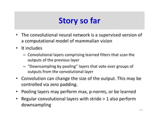
Story so far
•The convolutional neural network is a supervised version of
a computational model of mammalian vision
• It includes
– Convolutional layers comprising learned filters that scan the
outputs of the previous layer
– “Downsampling by pooling” layers that vote over groups of
outputs from the convolutional layer
• Convolution can change the size of the output. This may be
controlled via zero padding.
• Pooling layers may perform max, p-norms, or be learned
• Regular convolutional layers with stride > 1 also perform
downsampling
111
Preprocessing
• Large imagesare a problem
– Too much detail
– Will need big networks
• Typically scaled to small sizes, e.g. 128x128 or
even 32x32
– Based on how much will fit on your GPU
– Typically cropped to square images
– Filters are also typically square
116
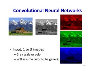
• Input isconvolved with a set of K1 filters
– Typically K1 is a power of 2, e.g. 2, 4, 8, 16, 32,..
– Filters are typically 5x5, 3x3, or even 1x1
Convolutional Neural Networks
K1 total filters
Filter size:
118
119.
• Input isconvolved with a set of K1 filters
– Typically K1 is a power of 2, e.g. 2, 4, 8, 16, 32,..
– Filters are typically 5x5, 3x3, or even 1x1
Convolutional Neural Networks
Small enough to capture fine features
(particularly important for scaled-down images)
K1 total filters
Filter size:
119
120.
• Input isconvolved with a set of K1 filters
– Typically K1 is a power of 2, e.g. 2, 4, 8, 16, 32,..
– Filters are typically 5x5, 3x3, or even 1x1
Convolutional Neural Networks
What on earth is this?
Small enough to capture fine features
(particularly important for scaled-down images)
K1 total filters
Filter size:
120
121.
• A 1x1filter is simply a perceptron that operates over the depth of the
stack of maps, but has no spatial extent
– Takes one pixel from each of the maps (at a given location) as input
– A non-distributed layer of the scanning MLP
The 1x1 filter
121
122.
• Input isconvolved with a set of K1 filters
– Typically K1 is a power of 2, e.g. 2, 4, 8, 16, 32,..
– Better notation: Filters are typically 5x5(x3), 3x3(x3), or
even 1x1(x3)
Convolutional Neural Networks
K1 total filters
Filter size:
122
123.
• Input isconvolved with a set of K1 filters
– Typically K1 is a power of 2, e.g. 2, 4, 8, 16, 32,..
– Better notation: Filters are typically 5x5(x3), 3x3(x3), or even 1x1(x3)
– Typical stride: 1 or 2
Convolutional Neural Networks
Total number of parameters:
Parameters to choose: , and
1. Number of filters
2. Size of filters
3. Stride of convolution
K1 total filters
Filter size:
123
124.
• The inputmay be zero-padded according to
the size of the chosen filters
Convolutional Neural Networks
K1 total filters
Filter size:
124
125.
• First convolutionallayer: Several convolutional filters
– Filters are “3-D” (third dimension is color)
– Convolution followed typically by a RELU activation
• Each filter creates a single 2-D output map
Convolutional Neural Networks
K1 filters of size:
𝐿 × 𝐿 × 3
𝑧 (𝑖, 𝑗) = 𝑤 𝑐, 𝑘, 𝑙 𝐼 𝑖 + 𝑘, 𝑗 + 𝑙 + 𝑏
( )
∈{ , , }
The layer includes a convolution operation
followed by an activation (typically RELU)
125
126.
Learnable parameters inthe first
convolutional layer
• The first convolutional layer comprises filters,
each of size
– Spatial span:
– Depth : 3 (3 colors)
• This represents a total of parameters
– “+ 1” because each filter also has a bias
• All of these parameters must be learned
126
127.
• First downsamplinglayer: From each block of each
map, pool down to a single value
– For max pooling, during training keep track of which position
had the highest value
Convolutional Neural Networks
𝐼/𝐷 × (𝐼/𝐷
Filter size:
𝐿 × 𝐿 × 3
pool
The layer pools PxP blocks
of into a single value
It employs a stride D between
adjacent blocks
∈ ( ),
∈ ( )
𝑋𝑤𝑖𝑛(𝑖) = [ 𝑖 − 1 𝐷 + 1, 𝑖 − 1 𝐷 + 𝑃]
𝑌𝑤𝑖𝑛(𝑗) = [ 𝑗 − 1 𝐷 + 1, 𝑗 − 1 𝐷 + 𝑃]
127
128.
• First downsamplinglayer: From each block of each
map, pool down to a single value
– For max pooling, during training keep track of which position
had the highest value
Convolutional Neural Networks
𝐼/𝐷 × (𝐼/𝐷
Filter size:
𝐿 × 𝐿 × 3
Parameters to choose:
Size of pooling block
Pooling stride
pool
Choices: Max pooling or
mean pooling?
Or learned pooling?
∈ ( ),
∈ ( )
𝑋𝑤𝑖𝑛(𝑖) = [ 𝑖 − 1 𝐷 + 1, 𝑖 − 1 𝐷 + 𝑃]
𝑌𝑤𝑖𝑛(𝑗) = [ 𝑗 − 1 𝐷 + 1, 𝑗 − 1 𝐷 + 𝑃]
128
129.
• First downsamplinglayer: From each block of each
map, pool down to a single value
– For max pooling, during training keep track of which position
had the highest value
𝐼/𝐷 × (𝐼/𝐷
Convolutional Neural Networks
Filter size:
𝐿 × 𝐿 × 3
pool
∈ ( ),
∈ ( )
𝑋𝑤𝑖𝑛(𝑖) = [ 𝑖 − 1 𝐷 + 1, 𝑖 − 1 𝐷 + 𝑃]
𝑌𝑤𝑖𝑛(𝑗) = [ 𝑗 − 1 𝐷 + 1, 𝑗 − 1 𝐷 + 𝑃]
129
130.
• First downsamplinglayer: From each block of each
map, pool down to a single value
– For max pooling, during training keep track of which position
had the highest value
Convolutional Neural Networks
𝐼/𝐷 × (𝐼/𝐷
Filter size:
𝐿 × 𝐿 × 3
pool
∈ ( ),
∈ ( )
𝑋𝑤𝑖𝑛(𝑖) = [ 𝑖 − 1 𝐷 + 1, 𝑖 − 1 𝐷 + 𝑃]
𝑌𝑤𝑖𝑛(𝑗) = [ 𝑗 − 1 𝐷 + 1, 𝑗 − 1 𝐷 + 𝑃]
𝐾 = 𝐾 . Just using the
new index 𝐾 for notational
uniformity.
Pooling layers do not change
the number of maps because
pooling is performed individually
on each of the maps in the
previous layer.
130
131.
• First poolinglayer: Drawing it differently for
convenience
Convolutional Neural Networks
1
1
𝐾1 × 𝐼 × 𝐼 𝐾2 × 𝐼/𝐷 × 𝐼/𝐷
2
131
132.
• First poolinglayer: Drawing it differently for
convenience
1
1
𝐾1 × 𝐼 × 𝐼 𝐾2 × 𝐼/𝐷 × 𝐼/𝐷
Convolutional Neural Networks
2
Jargon: Filters are often called “Kernels”
The outputs of individual filters are called “channels”
The number of filters ( 1, 2, etc) is the number of channels
132
133.
• Second convolutionallayer: 3-D filters resulting in 2-D maps
– Alternately, a kernel with output channels
Convolutional Neural Networks
2 3 3
3
3
( )
1
1
𝐾1 × 𝐼 × 𝐼 𝐾2 × 𝐼/𝐷 × 𝐼/𝐷
2
133
134.
• Second convolutionallayer: 3-D filters resulting in 2-D maps
2 3 3
3
3
( )
Convolutional Neural Networks
1
1
𝐾1 × 𝐼 × 𝐼 𝐾2 × 𝐼/𝐷 × 𝐼/𝐷
2
Total number of parameters:
All these parameters must be learned
Parameters to choose: , and
1. Number of filters
2. Size of filters
3. Stride of convolution
134
Convolutional Neural Networks
•This continues for several layers until the final convolved output is fed to
a softmax
– Or a full MLP
3
1
1
𝐾1 × 𝐼 × 𝐼
4
2 3 3
3
𝐾2 × 𝐼/𝐷 × 𝐼/𝐷
2
137
138.
The Size ofthe Layers
• Each convolution layer with stride 1 typically maintains the size of the image
– With appropriate zero padding
– If performed without zero padding it will decrease the size of the input
• Each convolution layer will generally increase the number of maps from the
previous layer
– Increasing layers reduces the amount of information lost by subsequent
downsampling
• Each pooling layer with stride decreases the size of the maps by a factor of
• Filters within a layer must all be the same size, but sizes may vary with layer
– Similarly for pooling, may vary with layer
• In general the number of convolutional filters increases with layers
138
139.
Parameters to choose(design choices)
• Number of convolutional and downsampling layers
– And arrangement (order in which they follow one another)
• For each convolution layer:
– Number of filters
– Spatial extent of filter
• The “depth” of the filter is fixed by the number of filters in the previous layer 𝐾
– The stride
• For each downsampling/pooling layer:
– Spatial extent of filter
– The stride
• For the final MLP:
– Number of layers, and number of neurons in each layer
139
Poll 4
141
What isthe relationship between the number of channels in the output of a convolutional layer and the
number of neurons in the corresponding layer of a scanning MLP
They are the same
The two are not related
Training
• Training isas in the case of the regular MLP
– The only difference is in the structure of the network
• Training examples of (Image, class) are provided
• Define a divergence between the desired output and true output of the
network in response to any input
• Network parameters are trained through variants of gradient descent
• Gradients are computed through backpropagation
1 2
3
143
144.
Learning the network
•Parameters to be learned:
– The weights of the neurons in the final MLP
– The (weights and biases of the) filters for every convolutional layer
3
1
1
𝐾1 × 𝐼 × 𝐼
3
learnable learnable
learnable
2 3 3
3
𝐾2 × 𝐼/𝐷 × 𝐼/𝐷
2
144
145.
Learning the CNN
•In the final “flat” multi-layer perceptron, all the weights and biases
of each of the perceptrons must be learned
• In the convolutional layers the filters must be learned
• Let each layer have maps
– is the number of maps (colours) in the input
• Let the filters in the th layer be size
• For the th layer we will require filter parameters
• Total parameters required for the convolutional layers:
∈
145
146.
Defining the loss
•The loss for a single instance
1
convolve convolve
Div()
d(x)
y(x)
Input: x
Div (y(x),d(x))
3
1
𝐾1 × 𝐼 × 𝐼
4
2 3 3
3
𝐾2 × 𝐼/𝐷 × 𝐼/𝐷
2
146
147.
Problem Setup
• Givena training set of input-output pairs
• The loss on the ith instance is
• The total loss
• Minimize w.r.t
147
148.
Training CNNs throughGradient Descent
• Gradient descent algorithm:
• Initialize all weights and biases
• Do:
– For every layer for all filter indices update:
•
• Until has converged
148
Total training loss:
Assuming the bias is also
represented as a weight
149.
Training CNNs throughGradient Descent
• Gradient descent algorithm:
• Initialize all weights and biases
• Do:
– For every layer for all filter indices update:
•
• Until has converged
149
Total training loss:
Assuming the bias is also
represented as a weight
Backpropagation: Final flatlayers
• Backpropagation continues in the usual manner
until the computation of the derivative of the
divergence w.r.t the inputs to the first “flat” layer
– Important to recall: the first flat layer is only the
“flattening” of the maps from the final convolutional
layer
( )
1 2
3
Conventional backprop until here
152
153.
Backpropagation: Convolutional and
Poolinglayers
• Backpropagation from the flat MLP requires
special consideration of
– The shared computation in the convolutional layers
– The pooling layers (particularly maxout)
1 2
3
Need adjustments here
( )
153
Learning the network
•Have shown the derivative of divergence w.r.t every intermediate output,
and every free parameter (filter weights)
• Can now be embedded in gradient descent framework to learn the
network
2
2
155
156.
Story so far
•The convolutional neural network is a supervised
version of a computational model of mammalian vision
• It includes
– Convolutional layers comprising learned filters that scan
the outputs of the previous layer
– Downsampling layers that operate over groups of outputs
from the convolutional layer to reduce network size
• The parameters of the network can be learned through
regular back propagation
– Continued in next lecture.. 156


![• First downsampling layer: From each block of each
map, pool down to a single value
– For max pooling, during training keep track of which position
had the highest value
Convolutional Neural Networks
𝐼/𝐷 × (𝐼/𝐷
Filter size:
𝐿 × 𝐿 × 3
pool
The layer pools PxP blocks
of into a single value
It employs a stride D between
adjacent blocks
∈ ( ),
∈ ( )
𝑋𝑤𝑖𝑛(𝑖) = [ 𝑖 − 1 𝐷 + 1, 𝑖 − 1 𝐷 + 𝑃]
𝑌𝑤𝑖𝑛(𝑗) = [ 𝑗 − 1 𝐷 + 1, 𝑗 − 1 𝐷 + 𝑃]
127](https://image.slidesharecdn.com/lec10-250803154459-b02f747c/85/lec10-CNN2-pdf-127-320.jpg)
![• First downsampling layer: From each block of each
map, pool down to a single value
– For max pooling, during training keep track of which position
had the highest value
Convolutional Neural Networks
𝐼/𝐷 × (𝐼/𝐷
Filter size:
𝐿 × 𝐿 × 3
Parameters to choose:
Size of pooling block
Pooling stride
pool
Choices: Max pooling or
mean pooling?
Or learned pooling?
∈ ( ),
∈ ( )
𝑋𝑤𝑖𝑛(𝑖) = [ 𝑖 − 1 𝐷 + 1, 𝑖 − 1 𝐷 + 𝑃]
𝑌𝑤𝑖𝑛(𝑗) = [ 𝑗 − 1 𝐷 + 1, 𝑗 − 1 𝐷 + 𝑃]
128](https://image.slidesharecdn.com/lec10-250803154459-b02f747c/85/lec10-CNN2-pdf-128-320.jpg)
![• First downsampling layer: From each block of each
map, pool down to a single value
– For max pooling, during training keep track of which position
had the highest value
𝐼/𝐷 × (𝐼/𝐷
Convolutional Neural Networks
Filter size:
𝐿 × 𝐿 × 3
pool
∈ ( ),
∈ ( )
𝑋𝑤𝑖𝑛(𝑖) = [ 𝑖 − 1 𝐷 + 1, 𝑖 − 1 𝐷 + 𝑃]
𝑌𝑤𝑖𝑛(𝑗) = [ 𝑗 − 1 𝐷 + 1, 𝑗 − 1 𝐷 + 𝑃]
129](https://image.slidesharecdn.com/lec10-250803154459-b02f747c/85/lec10-CNN2-pdf-129-320.jpg)
![• First downsampling layer: From each block of each
map, pool down to a single value
– For max pooling, during training keep track of which position
had the highest value
Convolutional Neural Networks
𝐼/𝐷 × (𝐼/𝐷
Filter size:
𝐿 × 𝐿 × 3
pool
∈ ( ),
∈ ( )
𝑋𝑤𝑖𝑛(𝑖) = [ 𝑖 − 1 𝐷 + 1, 𝑖 − 1 𝐷 + 𝑃]
𝑌𝑤𝑖𝑛(𝑗) = [ 𝑗 − 1 𝐷 + 1, 𝑗 − 1 𝐷 + 𝑃]
𝐾 = 𝐾 . Just using the
new index 𝐾 for notational
uniformity.
Pooling layers do not change
the number of maps because
pooling is performed individually
on each of the maps in the
previous layer.
130](https://image.slidesharecdn.com/lec10-250803154459-b02f747c/85/lec10-CNN2-pdf-130-320.jpg)


