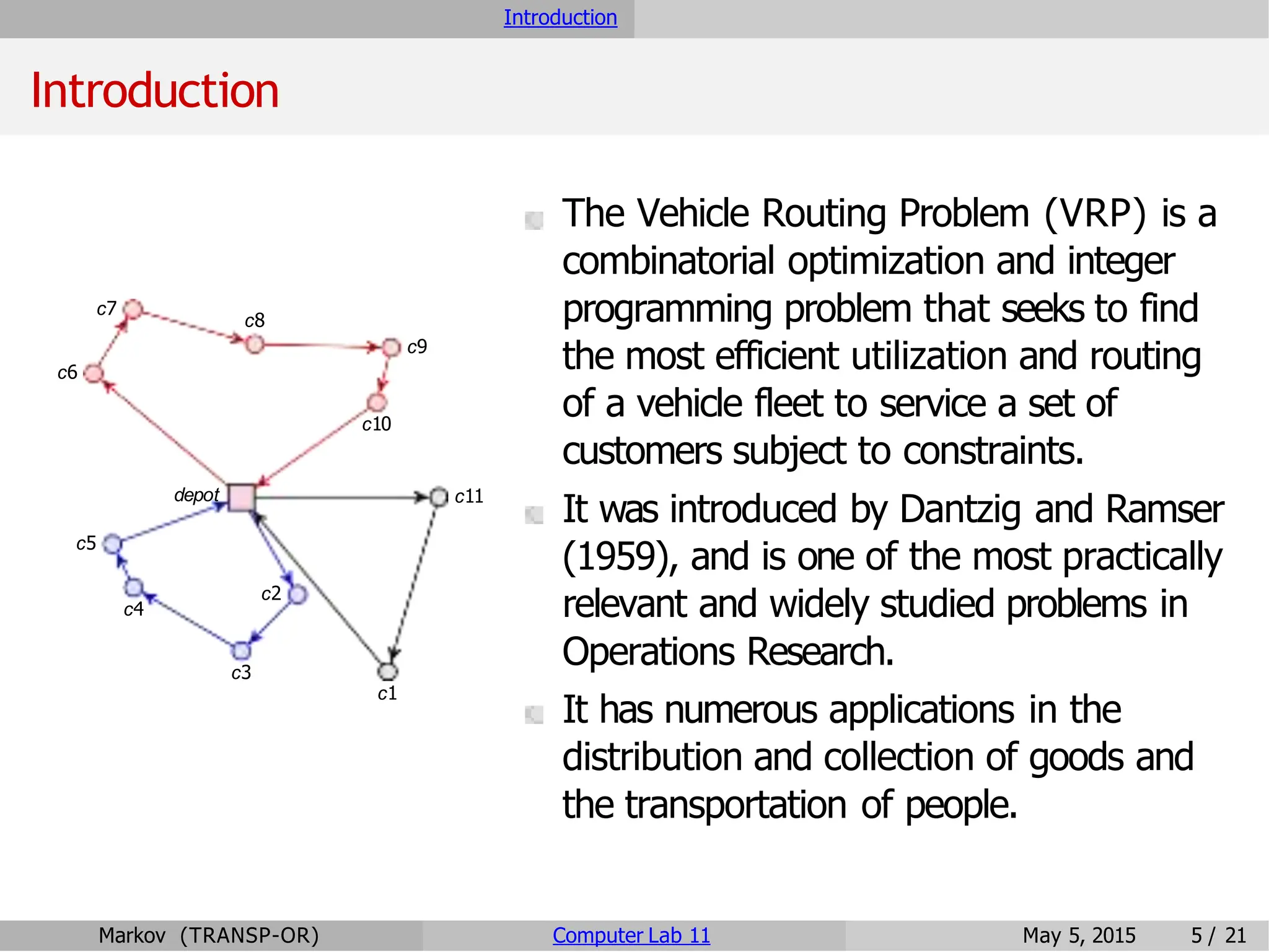
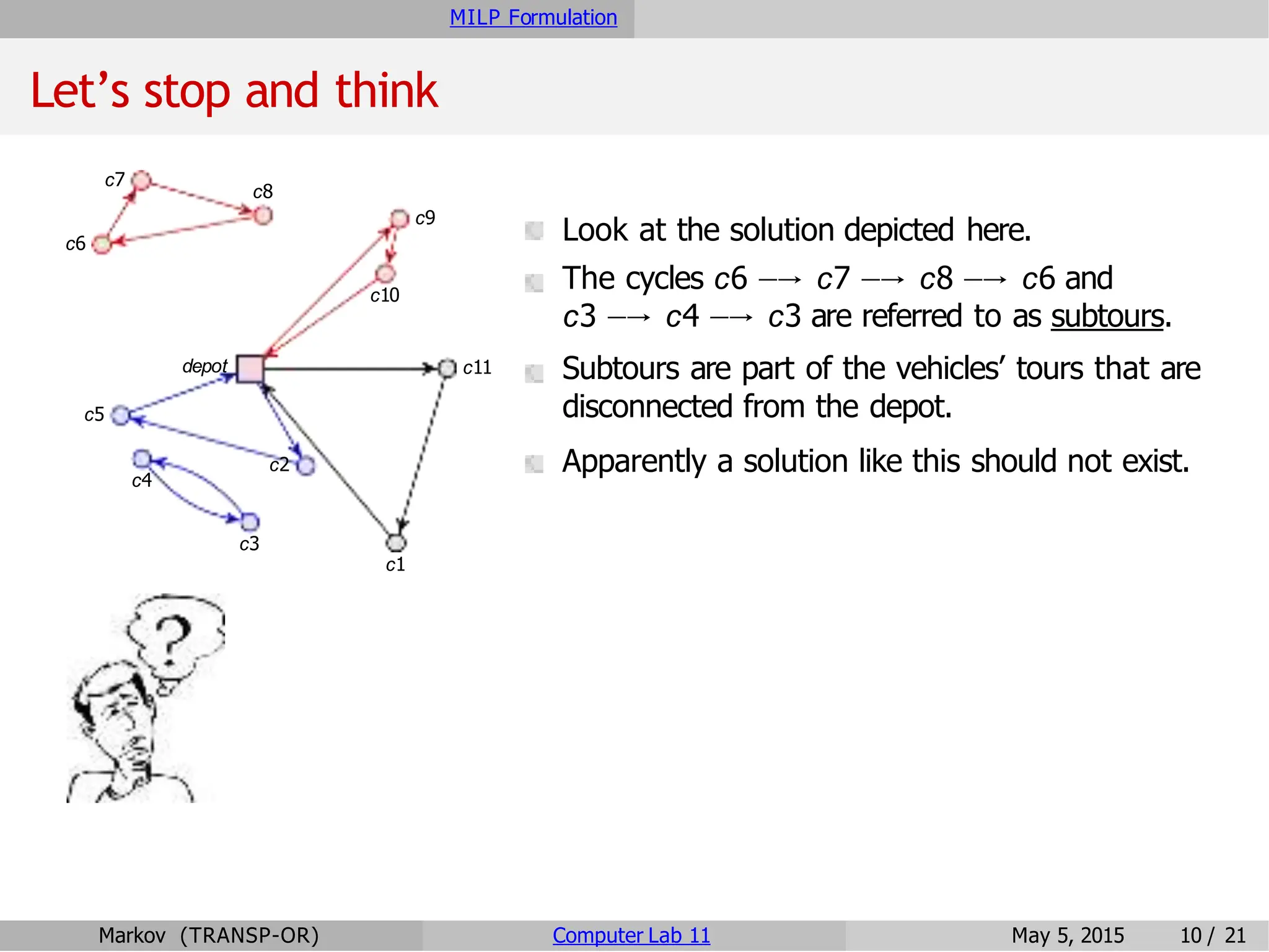
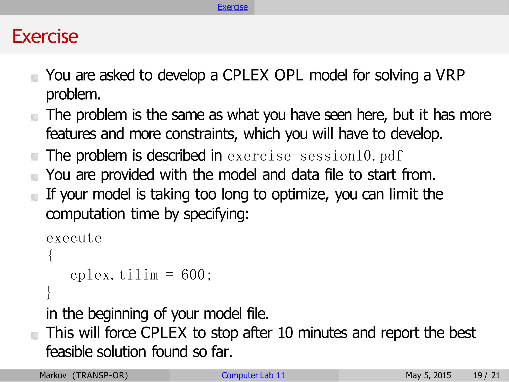
The Vehicle Routing Problem
Decision-aid Methodologies in Transportation: Computer Lab 11
Iliya Markov
Transport and Mobility Laboratory
School of Architecture, Civil and Environmental Engineering
École Polytechnique Fédérale de Lausanne
May 5, 2015
Markov (TRANSP-OR) Computer Lab 11 May 5, 2015 1 / 21
Overview
1 Introduction
2 MILP Formulation
3 Extensions
4 Solution approaches
5 Exercise
6 References
Markov (TRANSP-OR) Computer Lab 11 May 5, 2015 2 / 21
Introduction
Overview
1 Introduction
2 MILP Formulation
3 Extensions
4 Solution approaches
5 Exercise
6 References
Markov (TRANSP-OR) Computer Lab 11 May 5, 2015 3 / 21
Introduction
Introduction
Markov (TRANSP-OR) Computer Lab 11 May 5, 2015 4 / 21
Introduction
Introduction
depot c11
c10
c9
c8
c7
c6
c5
c4
c3
c2
c1
The Vehicle Routing Problem (VRP) is a
combinatorial optimization and integer
programming problem that seeks to find
the most efficient utilization and routing
of a vehicle fleet to service a set of
customers subject to constraints.
It was introduced by Dantzig and Ramser
(1959), and is one of the most practically
relevant and widely studied problems in
Operations Research.
It has numerous applications in the
distribution and collection of goods and
the transportation of people.
Markov (TRANSP-OR) Computer Lab 11 May 5, 2015 5 / 21
MILP Formulation
Overview
1 Introduction
2 MILP Formulation
3 Extensions
4 Solution approaches
5 Exercise
6 References
Markov (TRANSP-OR) Computer Lab 11 May 5, 2015 6 / 21
MILP Formulation
Formulating the capacitated VRP (CVRP)
We present the three-index directed vehicle-flow formulation of the
VRP, modified from Golden, Magnanti and Nguyen (1977). For it, we
need to define the following:
Sets:
K is a set of identical vehicles
N is a set of all nodes, where the depot is represented by two nodes, o
and d, for the start and end point of each tour
Parameters:
Q is the vehicle capacity
qi is the demand at node i
cij is the travel cost from node i to j
Variables:
xijk = 1 iff vehicle k moves from node i to j; 0 otherwise
yik = 1 iff vehicle k visits node i; 0 otherwise
uik is the cumulated demand serviced by vehicle k when arriving at
node i
Markov (TRANSP-OR) Computer Lab 11 May 5, 2015 7 / 21
MILP Formulation
Formulating the capacitated VRP (CVRP)
Objective: minimize total travel cost
Σ Σ Σ
minimize c x
k∈K i∈N j ∈N
ij ijk
Markov (TRANSP-OR) Computer Lab 11 May 5, 2015 8 / 21
MILP Formulation
Formulating the capacitated VRP (CVRP)
Objective: minimize total travel cost
Σ Σ Σ
minimize c x
k∈K i∈N j ∈N
A customer is visited by exactly one vehicle
ij ijk
Σ
k∈K
ik
s.t. y = 1, ∀
i ∈N  {o,d}
Markov (TRANSP-OR) Computer Lab 11 May 5, 2015 8 / 21
MILP Formulation
Formulating the capacitated VRP (CVRP)
Objective: minimize total travel cost
Σ Σ Σ
minimize c x
k∈K i∈N j ∈N
A customer is visited by exactly one vehicle
ij ijk
Σ
k∈K
ik
s.t. y = 1, ∀
i ∈N  {o,d}
Path-flow
s.t.
Σ
j ∈N{i}
ijk
x −
Σ
j ∈N{i}
xjik = 0, ∀
i ∈N  {o,d},k ∈K
∀
k ∈K
s.t.
Σ
j∈N{o}
ojk
x −
Σ
j∈N{o}
xjok = 1,
Markov (TRANSP-OR) Computer Lab 11 May 5, 2015 8 / 21
MILP Formulation
Formulating the capacitated VRP (CVRP)
Coupling
s.t. yik =
Σ
j ∈N{i}
xijk , ∀
i ∈N  {d},k ∈K
∀
k ∈K
s.t. ydk =
Σ
i∈N{d}
xidk,
Markov (TRANSP-OR) Computer Lab 11 May 5, 2015 9 / 21
MILP Formulation
Formulating the capacitated VRP (CVRP)
Coupling
s.t. yik =
Σ
j ∈N{i}
xijk , ∀
i ∈N  {d},k ∈K
∀
k ∈K
s.t. ydk =
Σ
i∈N{d}
xidk,
Domain
s.t. xijk ∈ {0,1}, ∀i,j ∈ N, k ∈ K
s.t. yik ∈ {0,1}, ∀i ∈ N, k ∈ K
Markov (TRANSP-OR) Computer Lab 11 May 5, 2015 9 / 21
MILP Formulation
Let’s stop and think
depot c11
c10
c9
c8
c7
c6
c5
c4
c3
c2
c1
Look at the solution depicted here.
The cycles c6 −→ c7 −→ c8 −→ c6 and
c3 −→ c4 −→ c3 are referred to as subtours.
Subtours are part of the vehicles’ tours that are
disconnected from the depot.
Apparently a solution like this should not exist.
Markov (TRANSP-OR) Computer Lab 11 May 5, 2015 10 / 21
MILP Formulation
Let’s stop and think
c9
c8
c7
c4
c6 Look at the solution depicted here.
c10 The cycles c6 −→ c7 −→ c8 −→ c6 and
c3 −→ c4 −→ c3 are referred to as subtours.
depot c11 Subtours are part of the vehicles’ tours that are
c5 disconnected from the depot.
c2 Apparently a solution like this should not exist.
However, is it a feasible solution for the model
c3
c1 defined above?
Let’s check constraint by constraint.
Markov (TRANSP-OR) Computer Lab 11 May 5, 2015 10 / 21
MILP Formulation
Let’s stop and think
depot c11
c10
c9
c8
c7
c6
c5
c4
c3
c2
c1
Σ Σ Σ
min c x
k∈K i∈N j ∈N
ij ijk
Σ
k∈K
ik
s.t. y = 1, ∀
i ∈ N  { o, d}
∀
i ∈ N  { o, d} , k ∈ K
∀
k ∈ K
∀
i ∈ N  { d} , k ∈ K
∀
k ∈ K
∀
i, j ∈ N, k ∈ K
∀
i ∈ N, k ∈ K
Σ
j ∈N { i} j ∈N { i}
ijk
x −
Σ
xjik = 0,
j∈N{o} j∈N{o}
xojk −
Σ Σ
xjok = 1,
Σ
ik ijk
y = x ,
j ∈N { i}
ydk =
Σ
xidk ,
i∈N { d}
xijk ∈ { 0, 1} ,
yik ∈ { 0, 1} ,
Markov (TRANSP-OR) Computer Lab 11 May 5, 2015 11 / 21
MILP Formulation
Subtour elimination constraints
The constraints we are missing are called
subtour elimination constraints (SEC).
Their role is to eliminate the possibility of subtours and to enforce the
vehicle capacity constraints.
SEC can be formulated in different ways, with an impact on the
number of SEC and the integrality gap.
Markov (TRANSP-OR) Computer Lab 11 May 5, 2015 12 / 21
MILP Formulation
Subtour elimination constraints
The constraints we are missing are called
subtour elimination constraints (SEC).
Their role is to eliminate the possibility of subtours and to enforce the
vehicle capacity constraints.
SEC can be formulated in different ways, with an impact on the
number of SEC and the integrality gap.
In the labs, we will focus on the so-called MTZ-formulation
introduced by Miller, Tucker and Zemlin (1960) for the TSP.
The first set of constraints links the node demand qi with the
cumulated demand uik in a big-M fashion:
s.t. uik + qj ≤ujk + Q(1 −xijk ), ∀
i,j ∈N,k ∈K
The second set of constraints enforces the vehicle capacity and
provides a lower bound for uik:
s.t. qi ≤uik ≤Q, ∀
i ∈N, k ∈K
Markov (TRANSP-OR) Computer Lab 11 May 5, 2015 12 / 21
MILP Formulation
Complete model
min
Σ Σ Σ
k∈K i∈N j ∈N
c x
ij ijk
Σ
k∈K
ik
s.t. y = 1, ∀
i ∈ N  { o, d}
∀
i ∈ N  { o, d} , k ∈ K
∀
k ∈ K
∀
i ∈ N  { d} , k ∈ K
∀
k ∈ K
∀
i, j ∈ N, k ∈ K
∀
i ∈ N, k ∈ K
∀
i, j ∈ N, k ∈ K
∀
i ∈ N, k ∈ K
xijk −
Σ Σ
j ∈N { i} j ∈N { i}
xjik = 0,
xojk −
Σ Σ
j∈N{o} j∈N{o}
xjok = 1,
yik =
Σ
j ∈N { i}
xijk ,
ydk =
Σ
i∈N { d}
xidk ,
uik + qj ≤ ujk + Q(1 − xijk ),
qi ≤ uik ≤ Q,
xijk ∈ { 0, 1} ,
yik ∈ { 0, 1} ,
Markov (TRANSP-OR) Computer Lab 11 May 5, 2015 13 / 21
Extensions
Overview
1 Introduction
2 MILP Formulation
3 Extensions
4 Solution approaches
5 Exercise
6 References
Markov (TRANSP-OR) Computer Lab 11 May 5, 2015 14 / 21
Extensions
Versions of the VRP
Many versions of the VRP have been considered in the literature
Capacitated VRP
VRP with time windows
Pickup and delivery VRP
VRP with backhauls
VRP with split deliveries
Periodic VRP
Heterogeneous fleet VRP
Dial-a-ride problem (DARP)
Stochastic VRP
Dynamic VRP
Inventory routing problem (IRP)
etc...
The interested student is referred to Toth and Vigo (2002) or Toth
and Vigo (2014). The full text of the former can be accessed online
from the EPFL library website if you are on campus or connected
through VPN.
Markov (TRANSP-OR) Computer Lab 11 May 5, 2015 15 / 21
Solution approaches
Overview
1 Introduction
2 MILP Formulation
3 Extensions
4 Solution approaches
5 Exercise
6 References
Markov (TRANSP-OR) Computer Lab 11 May 5, 2015 16 / 21
Solution approaches
Solution approaches
The VRP, and by generalization, all of its extensions are NP-hard.
Solution approaches can broadly be classified into three categories:
Exact approaches:
Branch-and-bound
Branch-and-cut
Branch-and-price-and-cut
Heuristic approaches:
Construction heuristics
Improvement heuristics
Metaheuristics–neighborhood based, population based
Hybridizations
Markov (TRANSP-OR) Computer Lab 11 May 5, 2015 17 / 21
Exercise
Overview
1 Introduction
2 MILP Formulation
3 Extensions
4 Solution approaches
5 Exercise
6 References
Markov (TRANSP-OR) Computer Lab 11 May 5, 2015 18 / 21
Exercise
Exercise
You are asked to develop a CPLEX OPL model for solving a VRP
problem.
The problem is the same as what you have seen here, but it has more
features and more constraints, which you will have to develop.
The problem is described in exercise-session10.pdf
You are provided with the model and data file to start from.
If your model is taking too long to optimize, you can limit the
computation time by specifying:
execute
{
cplex.tilim = 600;
}
in the beginning of your model file.
This will force CPLEX to stop after 10 minutes and report the best
feasible solution found so far.
Markov (TRANSP-OR) Computer Lab 11 May 5, 2015 19 / 21
References
Overview
1 Introduction
2 MILP Formulation
3 Extensions
4 Solution approaches
5 Exercise
6 References
Markov (TRANSP-OR) Computer Lab 11 May 5, 2015 20 / 21
References
Dantzig, G. and Ramser, R. (1959). The truck
dispatching problem. Management Science,
6:80–91.
Golden, B. L., Magnanti, T. L. and Nguyen, H. Q.
(1977). Implementing vehicle routing algorithms.
Networks, 7(2):133–148.
Miller, D.L.,Tucker, A.W., and Zemlin, R.A. (1960).
Integer programming formulations of traveling
salesman problems. Journal of the ACM, 326–329.
Toth, P and Vigo, D. (2002). The Vehicle Routing
Problem. SIAM.
Toth, P and Vigo, D. (2014). Vehicle Routing:
Problems, Methods, and Applications, Second
Edition. SIAM.
Markov (TRANSP-OR) Computer Lab 11 May 5, 2015 21 / 21

Lab11-Presentation_vehicule routing probleme.pptx

  • 1.
    The Vehicle RoutingProblem Decision-aid Methodologies in Transportation: Computer Lab 11 Iliya Markov Transport and Mobility Laboratory School of Architecture, Civil and Environmental Engineering École Polytechnique Fédérale de Lausanne May 5, 2015 Markov (TRANSP-OR) Computer Lab 11 May 5, 2015 1 / 21
  • 2.
    Overview 1 Introduction 2 MILPFormulation 3 Extensions 4 Solution approaches 5 Exercise 6 References Markov (TRANSP-OR) Computer Lab 11 May 5, 2015 2 / 21
  • 3.
    Introduction Overview 1 Introduction 2 MILPFormulation 3 Extensions 4 Solution approaches 5 Exercise 6 References Markov (TRANSP-OR) Computer Lab 11 May 5, 2015 3 / 21
  • 4.
  • 5.
    Introduction Introduction depot c11 c10 c9 c8 c7 c6 c5 c4 c3 c2 c1 The VehicleRouting Problem (VRP) is a combinatorial optimization and integer programming problem that seeks to find the most efficient utilization and routing of a vehicle fleet to service a set of customers subject to constraints. It was introduced by Dantzig and Ramser (1959), and is one of the most practically relevant and widely studied problems in Operations Research. It has numerous applications in the distribution and collection of goods and the transportation of people. Markov (TRANSP-OR) Computer Lab 11 May 5, 2015 5 / 21
  • 6.
    MILP Formulation Overview 1 Introduction 2MILP Formulation 3 Extensions 4 Solution approaches 5 Exercise 6 References Markov (TRANSP-OR) Computer Lab 11 May 5, 2015 6 / 21
  • 7.
    MILP Formulation Formulating thecapacitated VRP (CVRP) We present the three-index directed vehicle-flow formulation of the VRP, modified from Golden, Magnanti and Nguyen (1977). For it, we need to define the following: Sets: K is a set of identical vehicles N is a set of all nodes, where the depot is represented by two nodes, o and d, for the start and end point of each tour Parameters: Q is the vehicle capacity qi is the demand at node i cij is the travel cost from node i to j Variables: xijk = 1 iff vehicle k moves from node i to j; 0 otherwise yik = 1 iff vehicle k visits node i; 0 otherwise uik is the cumulated demand serviced by vehicle k when arriving at node i Markov (TRANSP-OR) Computer Lab 11 May 5, 2015 7 / 21
  • 8.
    MILP Formulation Formulating thecapacitated VRP (CVRP) Objective: minimize total travel cost Σ Σ Σ minimize c x k∈K i∈N j ∈N ij ijk Markov (TRANSP-OR) Computer Lab 11 May 5, 2015 8 / 21
  • 9.
    MILP Formulation Formulating thecapacitated VRP (CVRP) Objective: minimize total travel cost Σ Σ Σ minimize c x k∈K i∈N j ∈N A customer is visited by exactly one vehicle ij ijk Σ k∈K ik s.t. y = 1, ∀ i ∈N {o,d} Markov (TRANSP-OR) Computer Lab 11 May 5, 2015 8 / 21
  • 10.
    MILP Formulation Formulating thecapacitated VRP (CVRP) Objective: minimize total travel cost Σ Σ Σ minimize c x k∈K i∈N j ∈N A customer is visited by exactly one vehicle ij ijk Σ k∈K ik s.t. y = 1, ∀ i ∈N {o,d} Path-flow s.t. Σ j ∈N{i} ijk x − Σ j ∈N{i} xjik = 0, ∀ i ∈N {o,d},k ∈K ∀ k ∈K s.t. Σ j∈N{o} ojk x − Σ j∈N{o} xjok = 1, Markov (TRANSP-OR) Computer Lab 11 May 5, 2015 8 / 21
  • 11.
    MILP Formulation Formulating thecapacitated VRP (CVRP) Coupling s.t. yik = Σ j ∈N{i} xijk , ∀ i ∈N {d},k ∈K ∀ k ∈K s.t. ydk = Σ i∈N{d} xidk, Markov (TRANSP-OR) Computer Lab 11 May 5, 2015 9 / 21
  • 12.
    MILP Formulation Formulating thecapacitated VRP (CVRP) Coupling s.t. yik = Σ j ∈N{i} xijk , ∀ i ∈N {d},k ∈K ∀ k ∈K s.t. ydk = Σ i∈N{d} xidk, Domain s.t. xijk ∈ {0,1}, ∀i,j ∈ N, k ∈ K s.t. yik ∈ {0,1}, ∀i ∈ N, k ∈ K Markov (TRANSP-OR) Computer Lab 11 May 5, 2015 9 / 21
  • 13.
    MILP Formulation Let’s stopand think depot c11 c10 c9 c8 c7 c6 c5 c4 c3 c2 c1 Look at the solution depicted here. The cycles c6 −→ c7 −→ c8 −→ c6 and c3 −→ c4 −→ c3 are referred to as subtours. Subtours are part of the vehicles’ tours that are disconnected from the depot. Apparently a solution like this should not exist. Markov (TRANSP-OR) Computer Lab 11 May 5, 2015 10 / 21
  • 14.
    MILP Formulation Let’s stopand think c9 c8 c7 c4 c6 Look at the solution depicted here. c10 The cycles c6 −→ c7 −→ c8 −→ c6 and c3 −→ c4 −→ c3 are referred to as subtours. depot c11 Subtours are part of the vehicles’ tours that are c5 disconnected from the depot. c2 Apparently a solution like this should not exist. However, is it a feasible solution for the model c3 c1 defined above? Let’s check constraint by constraint. Markov (TRANSP-OR) Computer Lab 11 May 5, 2015 10 / 21
  • 15.
    MILP Formulation Let’s stopand think depot c11 c10 c9 c8 c7 c6 c5 c4 c3 c2 c1 Σ Σ Σ min c x k∈K i∈N j ∈N ij ijk Σ k∈K ik s.t. y = 1, ∀ i ∈ N { o, d} ∀ i ∈ N { o, d} , k ∈ K ∀ k ∈ K ∀ i ∈ N { d} , k ∈ K ∀ k ∈ K ∀ i, j ∈ N, k ∈ K ∀ i ∈ N, k ∈ K Σ j ∈N { i} j ∈N { i} ijk x − Σ xjik = 0, j∈N{o} j∈N{o} xojk − Σ Σ xjok = 1, Σ ik ijk y = x , j ∈N { i} ydk = Σ xidk , i∈N { d} xijk ∈ { 0, 1} , yik ∈ { 0, 1} , Markov (TRANSP-OR) Computer Lab 11 May 5, 2015 11 / 21
  • 16.
    MILP Formulation Subtour eliminationconstraints The constraints we are missing are called subtour elimination constraints (SEC). Their role is to eliminate the possibility of subtours and to enforce the vehicle capacity constraints. SEC can be formulated in different ways, with an impact on the number of SEC and the integrality gap. Markov (TRANSP-OR) Computer Lab 11 May 5, 2015 12 / 21
  • 17.
    MILP Formulation Subtour eliminationconstraints The constraints we are missing are called subtour elimination constraints (SEC). Their role is to eliminate the possibility of subtours and to enforce the vehicle capacity constraints. SEC can be formulated in different ways, with an impact on the number of SEC and the integrality gap. In the labs, we will focus on the so-called MTZ-formulation introduced by Miller, Tucker and Zemlin (1960) for the TSP. The first set of constraints links the node demand qi with the cumulated demand uik in a big-M fashion: s.t. uik + qj ≤ujk + Q(1 −xijk ), ∀ i,j ∈N,k ∈K The second set of constraints enforces the vehicle capacity and provides a lower bound for uik: s.t. qi ≤uik ≤Q, ∀ i ∈N, k ∈K Markov (TRANSP-OR) Computer Lab 11 May 5, 2015 12 / 21
  • 18.
    MILP Formulation Complete model min ΣΣ Σ k∈K i∈N j ∈N c x ij ijk Σ k∈K ik s.t. y = 1, ∀ i ∈ N { o, d} ∀ i ∈ N { o, d} , k ∈ K ∀ k ∈ K ∀ i ∈ N { d} , k ∈ K ∀ k ∈ K ∀ i, j ∈ N, k ∈ K ∀ i ∈ N, k ∈ K ∀ i, j ∈ N, k ∈ K ∀ i ∈ N, k ∈ K xijk − Σ Σ j ∈N { i} j ∈N { i} xjik = 0, xojk − Σ Σ j∈N{o} j∈N{o} xjok = 1, yik = Σ j ∈N { i} xijk , ydk = Σ i∈N { d} xidk , uik + qj ≤ ujk + Q(1 − xijk ), qi ≤ uik ≤ Q, xijk ∈ { 0, 1} , yik ∈ { 0, 1} , Markov (TRANSP-OR) Computer Lab 11 May 5, 2015 13 / 21
  • 19.
    Extensions Overview 1 Introduction 2 MILPFormulation 3 Extensions 4 Solution approaches 5 Exercise 6 References Markov (TRANSP-OR) Computer Lab 11 May 5, 2015 14 / 21
  • 20.
    Extensions Versions of theVRP Many versions of the VRP have been considered in the literature Capacitated VRP VRP with time windows Pickup and delivery VRP VRP with backhauls VRP with split deliveries Periodic VRP Heterogeneous fleet VRP Dial-a-ride problem (DARP) Stochastic VRP Dynamic VRP Inventory routing problem (IRP) etc... The interested student is referred to Toth and Vigo (2002) or Toth and Vigo (2014). The full text of the former can be accessed online from the EPFL library website if you are on campus or connected through VPN. Markov (TRANSP-OR) Computer Lab 11 May 5, 2015 15 / 21
  • 21.
    Solution approaches Overview 1 Introduction 2MILP Formulation 3 Extensions 4 Solution approaches 5 Exercise 6 References Markov (TRANSP-OR) Computer Lab 11 May 5, 2015 16 / 21
  • 22.
    Solution approaches Solution approaches TheVRP, and by generalization, all of its extensions are NP-hard. Solution approaches can broadly be classified into three categories: Exact approaches: Branch-and-bound Branch-and-cut Branch-and-price-and-cut Heuristic approaches: Construction heuristics Improvement heuristics Metaheuristics–neighborhood based, population based Hybridizations Markov (TRANSP-OR) Computer Lab 11 May 5, 2015 17 / 21
  • 23.
    Exercise Overview 1 Introduction 2 MILPFormulation 3 Extensions 4 Solution approaches 5 Exercise 6 References Markov (TRANSP-OR) Computer Lab 11 May 5, 2015 18 / 21
  • 24.
    Exercise Exercise You are askedto develop a CPLEX OPL model for solving a VRP problem. The problem is the same as what you have seen here, but it has more features and more constraints, which you will have to develop. The problem is described in exercise-session10.pdf You are provided with the model and data file to start from. If your model is taking too long to optimize, you can limit the computation time by specifying: execute { cplex.tilim = 600; } in the beginning of your model file. This will force CPLEX to stop after 10 minutes and report the best feasible solution found so far. Markov (TRANSP-OR) Computer Lab 11 May 5, 2015 19 / 21
  • 25.
    References Overview 1 Introduction 2 MILPFormulation 3 Extensions 4 Solution approaches 5 Exercise 6 References Markov (TRANSP-OR) Computer Lab 11 May 5, 2015 20 / 21
  • 26.
    References Dantzig, G. andRamser, R. (1959). The truck dispatching problem. Management Science, 6:80–91. Golden, B. L., Magnanti, T. L. and Nguyen, H. Q. (1977). Implementing vehicle routing algorithms. Networks, 7(2):133–148. Miller, D.L.,Tucker, A.W., and Zemlin, R.A. (1960). Integer programming formulations of traveling salesman problems. Journal of the ACM, 326–329. Toth, P and Vigo, D. (2002). The Vehicle Routing Problem. SIAM. Toth, P and Vigo, D. (2014). Vehicle Routing: Problems, Methods, and Applications, Second Edition. SIAM. Markov (TRANSP-OR) Computer Lab 11 May 5, 2015 21 / 21