1. Karanam Sekhara
Use of Analytics in Human Resources
A Sample of 1470 observations is taken, with
 Impact of Age, Gender, Education field, Marital Status, Monthly Income, Relationship
Satisfaction, Job Involvement, Job Level, Job Satisfaction, Percent Salary hike on Attrition
To study the above variable’s effect on attrition, T-Test (Numerical-Categorical) and Chi-Test
(Categorical- Categorical) are used.
 Age on Attrition
Age in this case is Numerical (integer) and Attrition is categorical (factor). As one of the variables is an
integer and the other one is a factor. We apply T-Test
Hypothesis
Null Hypothesis
(H0)
There is no significant difference between average age of the employees
who left the organisation and who are still working in organisation.
Alternate Hypothesis
(H1)
There is significant difference between average age of the employees
who left the organisation and who are still working in organisation.
Command: t.test(hrproject$Age~hrproject$Attrition)
Result:
t = 5.828, df = 316.93, p-value = 1.38e-08
95 percent confidence interval: 2.618930 5.288346
sample estimates: mean in group No Yes
37.56123 33.60759
Since p-value<0.05, we Reject H0 & Accept H1
Hence, there is significant difference between average age of the employees who left the
organisation and who are still working in organisation.
588
882
0
100
200
300
400
500
600
700
800
900
1000
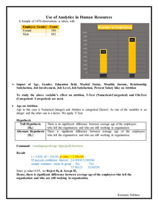
Female Male
Number of EmployeesEmployee Gender Count
Female 588
Male 882

2. Karanam Sekhara
 Gender on Attrition
Gender and Attrition are categorical (factor). As both variables are factor. We apply Chi-Square Test
Hypothesis
Null Hypothesis
(H0)
There is no association between gender and attrition
Alternate Hypothesis
(H1)
There is association between gender and attrition
Command: chisq.test(table(hrproject$Gender,hrproject$Attrition))
Result:
X-squared = 1.117, df = 1, p-value = 0.2906
Since p-value >0.05, we Accept H0
Hence, there is no association between gender and attrition
 Education field on Attrition
Both Education field and Attrition are categorical (factor). As both variables are factor, we apply Chi-
Square Test
Hypothesis
Null Hypothesis
(H0)
There is no association between Education field and attrition
Alternate Hypothesis
(H1)
There is association between Education field and attrition
Command: chisq.test(table(hrproject$EducationField,hrproject$Attrition))
Result:
X-squared = 16.025, df = 5, p-value = 0.006774
Since p-value <0.05, we Reject H0 & Accept H1
Hence, there is association between Education Field and Attrition

3. Karanam Sekhara
 Marital Status on Attrition
Both Marital Status and Attrition are categorical (factor). As both variables are factor, we apply Chi-
Square Test
Hypothesis
Null Hypothesis
(H0)
There is no association between Marital Status and attrition
Alternate Hypothesis
(H1)
There is association between Marital Status and attrition
Command: chisq.test(table(hrproject$MaritalStatus,hrproject$Attrition))
Result:
X-squared = 46.164, df = 2, p-value = 9.456e-11
Since p-value <0.05, we Reject H0 & Accept H1
Hence, there is association between Marital Status and Attrition
 Monthly Income on Attrition
Here monthly income is Numerical (integer) and Attrition is categorical (factor). As one of the variables
is an integer and the other one is a factor. We apply T-Test
Hypothesis
Null Hypothesis
(H0)
There is no significant difference between average monthly income of the
employees who left the organisation and who are still working in
organisation.
Alternate Hypothesis
(H1)
There is significant difference between average monthly income of the
employees who left the organisation and who are still working in
organisation.
Command: t.test(hrproject$MonthlyIncome~hrproject$Attrition)
Result: t = 7.4826, df = 412.74, p-value = 4.434e-13
95 percent confidence interval: 1508.244 2583.050
sample estimates: mean in group No Yes
6832.740 4787.093
Since p-value<0.05, we Reject H0 & Accept H1
Hence, there is significant difference between average monthly income of the employees who left
the organisation and who are still working in organisation.

4. Karanam Sekhara
 Relationship Satisfaction on Attrition
Here Relationship Satisfaction is Numerical (integer) and Attrition is categorical (factor). As one of the
variables is an integer and the other one is a factor. We apply T-Test
Hypothesis
Null Hypothesis
(H0)
There is no significant difference between average Relationship Satisfaction
of the employees who left the organisation and who are still working in
organisation.
Alternate Hypothesis
(H1)
There is significant difference between average Relationship Satisfaction of
the employees who left the organisation and who are still working in
organisation.
Command: t.test(hrproject$RelationshipSatisfaction~hrproject$Attrition)
Result:
t = 1.7019, df = 323.54, p-value = 0.08973
95 percent confidence interval: -0.02102367 0.29067575
sample estimates: mean in group No Yes
2.733982 2.599156
Since p-value>0.05, we Accept H0
Hence, there is significant difference between average Relationship Satisfaction of the employees
who left the organisation and who are still working in organisation.
 Job Involvement on Attrition
Here Job Involvement is Numerical (integer) and Attrition is categorical (factor). As one of the variables
is an integer and the other one is a factor. We apply T-Test
Hypothesis
Null Hypothesis
(H0)
There is no significant difference between average Job Involvement of the
employees who left the organisation and who are still working in
organisation.
Alternate Hypothesis
(H1)
There is significant difference between average Job Involvement of the
employees who left the organisation and who are still working in
organisation.
Command: t.test(hrproject$JobInvolvement~hrproject$Attrition)
Result: t = 4.6602, df = 312.81, p-value = 4.681e-06
95 percent confidence interval: 0.1453097 0.3576727
sample estimates: mean in group No Yes
2.770479 2.518987
Since p-value<0.05, we Reject H0 & Accept H1
Hence, there is significant difference between average age of the employees who left the
organisation and who are still working in organisation.

5. Karanam Sekhara
 Job Level on Attrition
Here Job Level is Numerical (integer) and Attrition is categorical (factor). As one of the variables is an
integer and the other one is a factor. We apply T-Test
Hypothesis
Null Hypothesis
(H0)
There is no significant difference between average Job Level of the
employees who left the organisation and who are still working in
organisation.
Alternate Hypothesis
(H1)
There is significant difference between average Job Level of the employees
who left the organisation and who are still working in organisation.
Command: t.test(hrproject$JobLevel~hrproject$Attrition)
Result: t = 7.3859, df = 376.25, p-value = 9.845e-13
95 percent confidence interval: 0.3733861 0.6443231
sample estimates: mean in group No Yes
2.145985 1.637131
Since p-value<0.05, we Reject H0 & Accept H1
Hence, there is significant difference between average Job Level of the employees who left the
organisation and who are still working in organisation.
 Job Satisfaction on Attrition
Here Job Satisfaction is Numerical (integer) and Attrition is categorical (factor). As one of the variables
is an integer and the other one is a factor. We apply T-Test
Hypothesis
Null Hypothesis
(H0)
There is no significant difference between average Job Satisfaction of the
employees who left the organisation and who are still working in
organisation.
Alternate Hypothesis
(H1)
There is significant difference between average Job Satisfaction of the
employees who left the organisation and who are still working in
organisation.
Command: t.test(hrproject$JobSatisfaction~hrproject$Attrition)
Result: t = 3.9261, df = 328.59, p-value = 0.0001052
95 percent confidence interval: 0.1547890 0.4656797
sample estimates: mean in group No Yes
2.778589 2.468354
Since p-value<0.05, we Reject H0 & Accept H1
There is significant difference between average Job Satisfaction of the employees who left the
organisation and who are still working in organisation.

6. Karanam Sekhara
 Percent Salary hike on Attrition
Here is Numerical (integer) and Attrition is categorical (factor). As one of the variables is an integer and
the other one is a factor. We apply T-Test
Hypothesis
Null Hypothesis
(H0)
There is no significant difference between average Percent Salary hike of the
employees who left the organisation and who are still working in
organisation.
Alternate Hypothesis
(H1)
There is significant difference between average Percent Salary hike of the
employees who left the organisation and who are still working in
organisation.
Command: t.test(hrproject$PercentSalaryHike~hrproject$Attrition)
Result:
t = 0.50424, df = 326.11, p-value = 0.6144
95 percent confidence interval: -0.3890709 0.6572652
sample estimates: mean in group No Yes
15.23114 15.09705
Since p-value>0.05, we Accept H0
There is no significant difference between average Percent Salary hike of the employees who left
the organisation and who are still working in organisation.
Descriptive Statistics,
1470 obs. of 35 variables, With 9 variables categorical and 26 variables Numerical type data.
Age Attrition Gender Department MaritalStatus
Minimum 18Years No: 1233 Female:588 H R 63 Divorced :327
Maximum 60Years Yes: 237 Male :882 R&D 961 Married :673
Sales 446 Single :470
HourlyRate MonthlyIncome OverTime
Min. : 30.00 Min. : 1009 No :1054
Median : 66.00 Median : 4919 Yes :416
Mean : 65.89 Mean : 6503
Max. :100.00 Max. :19999
EducationField JobRole
Human Resources 27 Sales Executive :326
Life Sciences 606 Research Scientist :292
Marketing 159 Laboratory Technician :259
Medical 464 Manufacturing Director :145
Other 82 Healthcare Representative :131
Technical Degree 132 Manager :102
(Other) :215

7. Karanam Sekhara
NumCompanies PercentSalary Performance Relationship
Worked Hike Rating Satisfaction
Min. :0.000 Min. :11.00 Min. :3.000 Min. :1.000
Median :2.000 Median :14.00 Median :3.000 Median :3.000
Mean :2.693 Mean :15.21 Mean :3.154 Mean :2.712
Max. :9.000 Max. :25.00 Max. :4.000 Max. :4.000
TotalWorkingYears TrainingTimesLastYear YearsAtCompany
Min. : 0.00 Min. :0.000 Min. : 0.000
Median :10.00 Median :3.000 Median : 5.000
Mean :11.28 Mean :2.799 Mean : 7.008
Max. :40.00 Max. :6.000 Max. : 40.000
YearsInCurrentRole YearsSinceLastPromotion YearsWithCurrManager
Min. : 0.000 Min. : 0.000 Min. : 0.000
Median : 3.000 Median : 1.000 Median : 3.000
Mean : 4.229 Mean : 2.188 Mean : 4.123
Max. :18.000 Max. :15.000 Max. :17.000
Cross Tabulations
Gender, Attrition
Command: table(hrdata$Gender,hrdata$Attrition)
Plot:
pie3D(theta=pi/4, explode=0.1,table(hrdata$Attrition),col=c("yellow","blue"),labels = names(table(hrda
ta$Attrition)),main="Employee Attrition")
barplot(beside=T,table(hrdata$Attrition,hrdata$Gender),xlab="Gender", ylab="No.of Employees",main
="Gender Wise Attrition",col=c("yellow","blue"))
Result:
No Yes
Female 501 87
Male 732 150
Attrition in Males is Higher than Females

8. Karanam Sekhara
Gender, Education Field
Command: table(hrdata$Gender,hrdata$EducationField)
Plot:
pie3D(theta=pi/4,explode=0.1,table(hrdata$EducationField),col=rainbow(6),labels=names(table(hrdata$
EducationField)),main="Employee Education ")
barplot(beside=T,table(hrdata$EducationField,hrdata$Gender),xlab="Gender", ylab="No.of Employees
",main="Gender Wise Education Field",col=rainbow(6))
Result:
Human Resources Life Sciences Marketing Medical Other Technical Degree
Female 8 240 69 190 29 52
Male 19 366 90 274 53 80
The contribution of Male Employees is more in Human Resources, Life Sciences, Technical Degree and
Other, while contribution of Female Employees is more in Marketing and Medical Education Fields

9. Karanam Sekhara
Gender, Job Satisfaction
Command: table(hrdata$Gender,hrdata$JobSatisfaction)
Plot:
pie3D(theta=pi/4,explode=0.1,table(hrdata$JobSatisfaction),col=rainbow(4),labels=names(table(hrdata$
JobSatisfaction)),main="Employee Job Satisfaction ")
barplot(beside=T,table(hrdata$JobSatisfaction,hrdata$Gender),xlab="Gender", ylab="No.of Employees
",main="Gender Wise Job Satisfacation",col = rainbow(4))
Result: 1 2 3 4
Female 119 118 181 170
Male 170 162 261 289
Job Satisfaction in case of Male Employees is more in level 3&4 compared to that of females by
2.6%

10. Karanam Sekhara
Gender, Marital Status, Attrition
Command: table(hrdata$Gender,hrdata$MaritalStatus,hrdata$Attrition)
Plot:
pie3D(theta=pi/4,explode=0.1,table(hrdata$MaritalStatus),col=c("Red","yellow","green"),labels=names
(table(hrdata$MaritalStatus)),main="Employee Marital Status")
barplot(beside=T,table(hrdata$MaritalStatus,hrdata$Attrition),xlab="Attrition", ylab="No. of Employee
s",main="Marital Status Wise Attrition",col=c("Red","yellow","green"))
Result:
No Yes
Divorced Married Single Divorced Married Single
Female 108 241 152 9 31 47
Male 186 348 198 24 53 73
Attrition in Male Employees is more compared to Females Employees in every Marital Status Category,
But, attrition in case of Marital Status -Single Category is almost same at 9%.

11. Karanam Sekhara
Gender, Department, Attrition
Command: table(hrdata$Gender,hrdata$Department,hrdata$Attrition)
Plot:
pie3D(theta=pi/4,explode=0.1,table(hrdata$Department),col=c("Red","yellow","green"),labels=names(t
able(hrdata$Department)),main="Employee Departments")
barplot(beside=T,table(hrdata$Department,hrdata$Attrition),xlab="Attrition", ylab="No. of Employees"
,main="Employee Departments Wise Attrition",col=c("Red","yellow","green"))
Result: No Yes
HR R & D Sales HR R & D Sales
Female 14 336 151 6 43 38
Male 37 492 203 6 90 54
Major Attrition is from R&D and Sales with Female Employee’s attrition being more in Sales compared
to Male Employees by 0.3%.

12. Karanam Sekhara
Hypothesis tests and analysis
i. Gender vs Percent Salary Hike
Here Percent Salary Hike is Numerical (integer) and Gender is categorical (factor). As one of the
variables is an integer and the other one is a factor, so we apply T-Test
Hypothesis
Null Hypothesis
(H0)
There is no significant difference between average Percent Salary Hike of the
female and male employees.
Alternate Hypothesis
(H1)
There is significant difference between average Percent Salary Hike of the
female and male employees.
Command: t.test(hrproject$PercentSalaryHike~hrproject$Gender)
Result: t = -0.10432, df = 1242.4, p-value = 0.9169
95 percent confidence interval: -0.4041984 0.3633821
sample estimates: mean in group Female mean in group Male
15.19728 15.21769
Since p-value>0.05, we Accept H0
There is no significant difference between average Percent Salary Hike of female and male
employees.
ii. Gender vs Job Satisfaction
Here Job Satisfaction is Numerical (integer) and Gender is categorical (factor). As one of the
variables is an integer and the other one is a factor. We apply T-Test
Hypothesis
Null Hypothesis
(H0)
There is no significant difference between average Job Satisfaction of female
employees and male employees.
Alternate Hypothesis
(H1)
There is significant difference between average Job Satisfaction of female
employees and male employees.
Command: t.test(hrproject$JobSatisfaction~hrproject$Gender)
Result:
t = -1.2773, df = 1266.6, p-value = 0.2017
95 percent confidence interval: -0.18976672 0.04010685
sample estimates: mean in group Female mean in group Male
2.683673 2.758503
Since p-value>0.05, we Accept H0
There is no significant difference between average Job Satisfaction of female and male
employees.

13. Karanam Sekhara
iii. Job Involvement Vs Job Satisfaction
Here both Job Involvement and Job Satisfaction are Numerical (integer) type data, so we apply
correlation to find the relationship.
Hypothesis
Null Hypothesis
(H0)
There is no correlation between Job Involvement and Job Satisfaction of the
employees.
Alternate Hypothesis
(H1)
There is correlation between Job Involvement and Job Satisfaction of the
employees.
Command: cor.test(hrproject$JobInvolvement,hrproject$JobSatisfaction)
Result: t = -0.82303, df = 1468, p-value = 0.4106
95 percent confidence interval: -0.07252374 0.02968414
sample estimates: cor
-0.02147591
Since p-value>0.05, we Accept H0
i. There is no correlation (almost zero) between Job Involvement and Job Satisfaction of the
employees. Job Involvement and Job Satisfaction are weakly correlated with negative side.
ii. Marital Status vs Job Satisfaction
Here Percent Salary Hike is Numerical (integer) and Education Field is multi-level categorical
(factor). So, we apply One Way ANOVA Test.
Hypothesis
Null Hypothesis
(H0)
There is no significant difference of means among and between Education
Field and Percent Salary Hike of the employees.
Alternate Hypothesis
(H1)
There is significant difference of means among and between Education Field
and Percent Salary Hike of the employees.
Command: aov(hrproject$JobSatisfaction~hrproject$MaritalStatus)
summary(aov(hrproject$JobSatisfaction~hrproject$MaritalStatus))
Result: Terms:
hrproject$MaritalStatus Residuals
Sum of Squares 1.1577 1785.5423
Deg. of Freedom 2 1467
Residual standard error: 1.10324
Summary:
Df Sum Sq Mean Sq F value Pr(>F)
MaritalStatus 2 1.2 0.5789 0.476 0.622
Residuals 1467 1785.5 1.2171
Since Pr-value>0.05, we Accept H0
There is no significant difference of means among and between Education Field and
Percent Salary Hike of the employees.

14. Karanam Sekhara
iii. Education Field Vs Percent Salary Hike
Here Percent Salary Hike is Numerical (integer) and Education Field is multi-level categorical
(factor). So, we apply One Way ANOVA Test.
Hypothesis
Null Hypothesis
(H0)
There is no significant difference of means among and between Education
Field and Percent Salary Hike of the employees.
Alternate Hypothesis
(H1)
There is significant difference of means among and between Education Field
and Percent Salary Hike of the employees.
Command: aov(hrproject$PercentSalaryHike~hrproject$EducationField)
summary(aov(hrproject$PercentSalaryHike~hrproject$EducationField))
Result: Terms:
hrproject$EducationField Residuals
Sum of Squares 70.722 19606.745
Deg. of Freedom 5 1464
Residual standard error: 3.659588
Summary:
Df Sum Sq Mean Sq F value Pr(>F)
EducationField 5 71 14.14 1.056 0.383
Residuals 1464 19607 13.39
Since Pr-value>0.05, we Accept H0
There is no significant difference of means among and between Education Field and
Percent Salary Hike of the employees.
iv. Job Satisfaction Vs Age
Here Job Satisfaction and Age both are Numerical (integer) type data so, we apply correlation test.
Hypothesis
Null Hypothesis
(H0)
There is no correlation between Job Satisfaction and Age of the employees.
Alternate Hypothesis
(H1)
There is correlation between Job Satisfaction and Age of the employees.
Command: cor.test(hrproject$Age,hrproject$JobSatisfaction)
Result: t = -0.18743, df = 1468, p-value = 0.8513
95 percent confidence interval: -0.05600533 0.04624715
sample estimates: cor
-0.004891877
Since p-value>0.05, we Accept H0
There is no correlation (almost zero) between Age and Job Satisfaction of the employees.
In this case, Job Satisfaction and Age are weakly correlated and is negative

15. Karanam Sekhara
Multiple Linear Regression
Command:
Regression Model 1
hrdatareg1=lm(MonthlyIncome~Gender+EducationField+JobInvolvement+JobLevel+Perce
ntSalaryHike+JobRole+performanceratingfactor+YearsAtCompany+OverTime+YearsInCur
rentRole,data=hrdata)
Regression Model 2
Hrdatareg2=lm(MonthlyIncome~MonthlyRate+Department+JobLevel+EducationField+JobI
nvolvement+JobRole+YearsAtCompany,data=hrdata)
Regression Model 3
hrdatareg3=lm(MonthlyIncome~MonthlyRate+JobLevel+JobInvolvement+JobRole+YearsA
tCompany,data=hrdata)
summary(hrdatareg3)
plot(hrdatareg3)
Output:
After removing the insignificant factors from Regression Model 1 & 2, we have a Multiple R-Squared
value of 94.2% in Regression Model 3.
Residuals:
Min 1Q Median 3Q Max
-3743.1 -676.2 -31.3 675.9 4136.1
Coefficients:
Estimate Std. Error t value Pr(>|t|)
(Intercept) 3.168e+02 2.156e+02 1.469 0.141956
MonthlyRate -4.417e-03 4.187e-03 -1.055 0.291629
JobLevel 2.996e+03 5.830e+01 51.388 < 2e-16 ***
JobInvolvement -8.887e+01 4.189e+01 -2.121 0.034061 *
JobRoleHuman Resources -2.868e+02 1.944e+02 -1.475 0.140373
JobRoleLaboratory Technician -5.562e+02 1.395e+02 -3.987 7.02e-05 ***
JobRoleManager 4.097e+03 1.805e+02 22.703 < 2e-16 ***
JobRoleManufacturing Director -1.528e+02 1.373e+02 -1.112 0.266205
JobRoleResearch Director 3.979e+03 1.819e+02 21.879 < 2e-16 ***
JobRoleResearch Scientist -4.343e+02 1.385e+02 -3.136 0.001746 **
JobRoleSales Executive -1.598e+02 1.181e+02 -1.353 0.176162
JobRoleSales Representative -6.786e+02 1.768e+02 -3.838 0.000129 ***
YearsAtCompany 1.297e+01 5.812e+00 2.232 0.025792 *
---
Signif. codes: 0 ‘***’ 0.001 ‘**’ 0.01 ‘*’ 0.05 ‘.’ 0.1 ‘ ’ 1
Multiple R-squared: 0.942, Adjusted R-squared: 0.9415
F-statistic: 1971 on 12 and 1457 DF, p-value: < 2.2e-16

16. Karanam Sekhara
Below graphs show the effect of various variables on Monthly Income of the Employee
Regression Model 3 is a good fit for explaining the various variables which have effect the monthly
income. But, all Job Roles comparatively don’t have significate effect in Regression Model 3, like
Human Resources, Manufacturing Director and Sales Executive Job Roles don’t have much effect.
After considering the significate variables we have the following equation has regression equation
Monthly Income= 3.168e+02+2.996e+03*(JobLevel) - 8.887e+01*(JobInvolvement) - 5.562e+02*(JobRole
LaboratoryTechnician) + 4.097e+03*(JobRoleManager)+ 3.979e+03*(JobRoleResearch
Director) -4.343e+02*(JobRoleResearch Scientist) - 6.786e+02*(JobRoleSales
Representative).
For every positive and negative coefficient there is a corresponding increase and decrease in monthly
Income ofthe employees.

17. Karanam Sekhara
Conduct Decision Tree Analysis and Logistic Regressionand predict the accuracy
Command For Decision Tree Analysis:
hrdatarpart=rpart(Attrition~.,data=hrdata)
plot(hrdatarpart, uniform=TRUE,main="Attrition Desicion Tree")
text(hrdatarpart, use.n=TRUE, all=TRUE,cex=1.01)
Command For Accurancy:
hrdatactreepredict=predict(hrdatactree,type="response")
table(hrdata$Attrition,hrdatactreepredict)
(1157+100)/(1157+76+137+100)
Result:
From above Decision Tree, we know that 237 employees left the company.
 110 employees having working year more than 2.5 years. Out of 110 employees, 27 left due to Job Role
out of which 17 were unhappy with hourly rates.
 127 employees left due to overtime, out of which 48 had monthly income more than Rs.2475. And out of
48 employees 36 were unhappy with daily rates and 12 due to years spent in current role. Remaining
employees who had monthly income less than Rs. 2475 left company due Stock option level (37),
monthly rate (21) and training times last year (16).
Hence we can say that out of 237 employees, 81 left company due to job roles. So, company
management should consider the overtime, job roles, stock options and monthly rates.
Accuracy Result: the accuracy of this model is 85%
No Yes
No 1157 76
Yes 137 100
(1157+100)/(1157+76+137+100) = 0.8551020408

18. Karanam Sekhara
Command for Logistic Regression:
hrdata1=data.frame(hrdata$Attrition,hrdata$MonthlyIncome,hrdata$Gender,hrdata$EducationField,
hrdata$JobInvolvement,hrdata$JobLevel,hrdata$PercentSalaryHike,hrdata$JobRole,
hrdata$performanceratingfactor,hrdata$YearsAtCompany,hrdata$OverTime,
hrdata$YearsInCurrentRole)
str(hrdata1)
hrdatalogit=glm(Attrition~MonthlyIncome+annualincome+OverTime+TotalWorkingYears,data=hrdata,
family="binomial")
summary(hrdatalogit)
hrdatalogitpredict=predict(hrdatalogit,type="response")
table(hrdata1$hrdata.Attrition,hrdatalogitpredict>0.5)
(1232+5)/(1+232+1232+5)
Result:
Deviance Residuals:
Min 1Q Median 3Q Max
-1.1808 -0.5712 -0.4672 -0.2783 2.9683
Coefficients: (1 not defined because of singularities)
Estimate Std. Error z value Pr(>|z|)
(Intercept) -1.258e+00 1.534e-01 -8.199 2.43e-16 ***
MonthlyIncome -6.808e-05 3.088e-05 -2.205 0.02746 *
annualincome NA NA NA NA
OverTimeYes 1.396e+00 1.508e-01 9.258 < 2e-16 ***
TotalWorkingYears -5.408e-02 1.745e-02 -3.099 0.00194 **
---
Signif. codes: 0 ‘***’ 0.001 ‘**’ 0.01 ‘*’ 0.05 ‘.’ 0.1 ‘ ’ 1
(Dispersion parameter for binomial family taken to be 1)
Null deviance: 1298.6 on 1469 degrees of freedom
Residual deviance: 1157.6 on 1466 degrees of freedom
AIC: 1165.6
Number of Fisher Scoring iterations: 5
FALSE TRUE
No 1232 1
Yes 232 5
(1232+5)/(1+232+1232+5)
0.8394211
 For a one unit decrease in MonthlyIncome there is decrease of 6.808e-05 in attrition.
 For a one unit decrease in TotalWorkingYears there is decrease of 5.408e-02 in attrition.
 For 1 unit increase in OverTimeYes, there is an increase of 1.396e+00 in attrition.
 This logistic regression model has an accuracy of 83.9%