INTRODUCTION TO MACHINE LEARNING FOR MATERIALS SCIENCE

3/5/24, 9:02 PM .intromllab-0
https://proxy.nanohub.org/weber/2367463/J0nPMJG4WA0CGdrv/7/apps/intromllab.ipynb?appmode_scroll=13804 1/52
INTRODUCTION TO MACHINE LEARNING FOR MATERIALS SCIENCE
LAB ACTIVITY
Authors: Ben Afflerbach, Computational Materials Group, University of Wisconsin–Madison, and Rundong Jiang, Citrine Informatics
This lab introduces students to an end-to-end example of applying a machine learning (ML) workflow to a materials science dataset to address a
research problem. The lab aims at deepening the conceptual understanding of ML, and while procedural skills such as writing Python code are
not the focus of this lab, students will gain experience with a number of standard open source packages by interacting with code snippets
through the Jupyter Notebook format and describing what each essential command does.
If you're unfamiliar with Jupyter Notebooks, take a moment to read about the lesson format. Otherwise, go through the "prerequisites" section
and click the "begin lesson" button below to get started!

PREREQUISITES
SAVING YOUR WORK ON NANOHUB
This is a hosted Jupyter Notebook on Nanohub. Any edits you've made to this notebook will not be carried over! So it's encouraged to make the
copy first and then work through the lab in that copied version.
You can do that by selecting File -> Make a Copy in the top left of the page.
Once you've made a copy, you can save that copy by clicking the save button again in the top left of the page.
When you make that copy, you'll have to go through a slightly different proccess to access the copied verison:
Launch the baseline "Jupyter Notebook" tool on Nanohub: https://nanohub.org/resources/jupyter
(https://nanohub.org/resources/jupyter)
Once you have that open, navigate in the file tree and open the notebook: Data -> Results -> (Most Recent Session Number) -> introml1ab -
> bin -> intromllab-Copy1.ipynb
PRIOR KNOWLEDGE
This lab activity is appropriate for students with a good conceptual understanding of a materials-focused machine learning workflow. For
example, you should feel comfortable:
listing key components of a ML workflow
explaining the importance of featurization / feature generation for materials data
identifying the relationship between cross-validation and overfitting
distinguishing between a parameter and a hyperparameter
evaluating model performance using common error metrics
Feel free to use modules 1-6 of "Introduction to Machine Learning for Materials Science" as a refresher, before proceeding with this lab. This is a
series of slide decks included under "supporting docs" on the tool's webpage www.nanohub.org/tools/intromllab
(http://www.nanohub.org/tools/intromllab)

TABLE OF CONTENTS
LESSON FORMAT
JUPYTER NOTEBOOKS TIPS AND TRICKS
SECTION 0: SETUP
SECTION 1: DATA INSPECTION
IMPORTING DATASET
Exercise 1.1
DATA CLEANING
Exercise 1.2
Exercise 1.3
EVALUATING DATA AVAILABILITY
Exercise 1.4
Exercise 1.5
Exercise 1.6
SECTION 2: FEATURE GENERATION
MASTML CONFIGURATION
UNDERSTANDING COMPOSITIONAL AVERAGE FEATURES
Exercise 2.1

SECTION 3: FEATURE ENGINEERING
REMOVE CONSTANT COLUMNS
Exercise 3.1
REMOVE HIGHLY CORRELATED COLUMNS
Exercise 3.2
FEATURE NORMALIZATION
SECTION 4: SETUP FOR MODEL EVALUATION
ESTABLISHING TRAIN/TEST SPLIT
EVALUATING TRAIN/TEST SPLIT
Exercise 4.1
SECTION 5: FITTING AND EVALUATING A DEFAULT MODEL
FITTING THE DECISION TREE MODEL
EVALUATING MODEL PERFORMANCE ON TRAINING DATA
Exercise 5.1
EVALUATING MODEL PERFORMANCE ON TEST DATA
Exercise 5.2

SECTION 6: HYPERPARAMETER OPTIMIZATION
ESTABLISHING A CROSS-VALIDATION SCHEME
DEFINING A PARAMETER SPACE
SETTING UP A GRID SEARCH
Exercise 6.1
VISUALIZING BIAS-VARIANCE TRADEOFF
Exercise 6.2
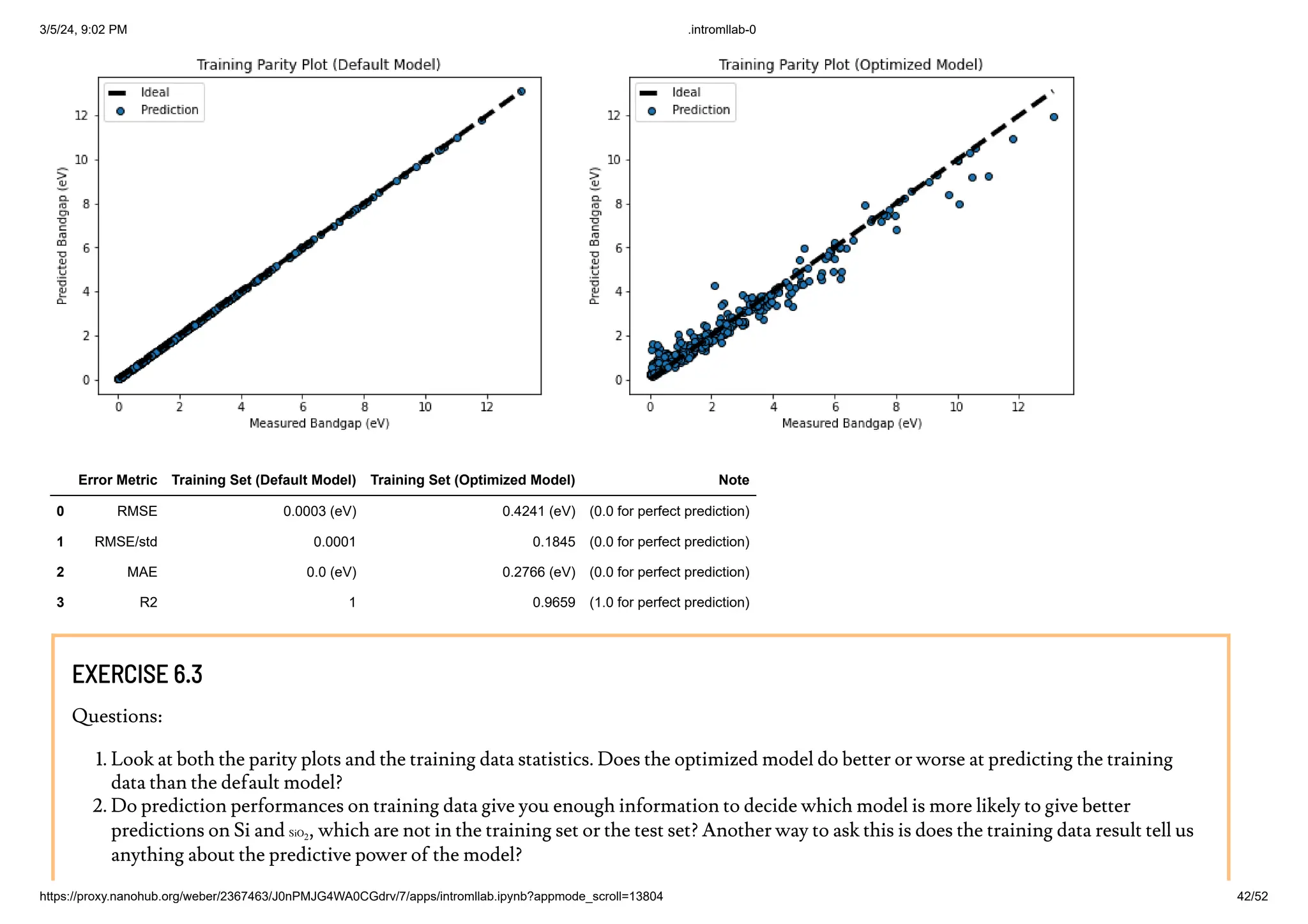
DEFAULT VS. OPTIMIZED MODEL: TRAINING AND VALIDATION DATA PERFORMANCE
Exercise 6.3
DEFAULT VS. OPTIMIZED MODEL: TEST DATA PERFORMANCE
Exercise 6.4
Exercise 6 5
[-----------------------------------BEGIN LESSON----------------
-------------------]
LESSON FORMAT
This is a Jupyter Notebook. It allows you to interact with this page by writing and running code. As you move through this notebook, you
will see unique sections. Within each section, there are learning goals for the section, an overview of the content covered in each section,
and then the content for the section itself. This content can take the form of written lessons, code examples, or coding exercises. The
instructions for the coding exercises are wrapped in an orange rectangle. These instructions will be followed by a code block that resembles
this:

### FINISH THE CODE BELOW ###
[Your code goes here]
#---------------------------#
Throughout this notebook you'll also see green boxes with the title ProTip that look much like this one. These boxes contain inportant
helpful information
JUPYTER NOTEBOOK TIPS AND TRICKS
CELLS
Each individual part of this notebook is known as a cell. The orange highlight bar along the left edge of this page indicates which cell is
active.
MOVING BETWEEN ACTIVE CELLS
You can move between cells by hitting the up and down arrows or by clicking on the cell you want to focus on. The up and down arrow
keys will only move you between cells when you are not in edit mode.
EDIT MODE
Hit the enter key on the active cell to "enter" it and edit its contents. While in edit mode, the up and down arrow keys will not move you
between cells. Double clicking a cell will also enable edit mode.
RUNNING A CELL
Hit shift + enter to run the active cell. In a code cell, the code will run and if there is output, it will be displayed immediately below the
code cell. In a markdown cell, the markdown will be rendered. Running a cell will automatically make the following cell the new active cell.
EXIT EDIT MODE

If you're editing a cell and want to exit edit mode, hit the esc key. This will exit edit mode, but the current cell will still be the active cell.
This action will not run the cell. It will enable you to use the up and down arrow keys to move between cells again.
ADDING A CELL
When you're not in edit mode, hit b to add a new cell. The new cell will be added directly below the active cell.
DELETING A CELL
When you're not in edit mode, hit x to delete the active cell.
SWITCHING BETWEEN MARKDOWN AND CODE
When you're not in edit mode, you can convert a code cell to a markdown cell by hitting the m key, and convert a markdown cell to a code
cell by hitting the c key.
SETUP
Back to TOC
LEARNING OUTCOMES
1. Describe the purpose of essential Python packages used in this lab
2. Recall that helper functions are available in this lab
PYTHON PACKAGES
There are a number of Python packages we'll use throughout the lab. Each of the import statements below imports or loads these packages in so
that we can use them. A brief description is given for each one.

HELPER FUNCTIONS
The final import we'll do is import some custom functions that mainly put together the plots and some specific analysis that we'll use throughout
the lab. If you're interested in learning what exactly these look like you can open up the helper_functions.py text file that is in the same folder as
this notebook.
There are a number of steps we'll take which would normally have a random state. In order to have consistent results we'll fix them all by setting
a random seed for all those processes.
MATERIALS BACKGROUND
Back to TOC
BAND GAP DATASET
Throughout the lab we'll be working with a digitized version of a band gap dataset compiled by two scientists, W.H. Strehlow and E.L. Cook.
They compiled this dataset of elementary and binary compound semiconductors in 1973 by searching through 723 individual references. Along
with simply compiling reported measurements they also took the time to identify more and less reliable data points by taking "into consideration
the material, the method of measurement, the reported sample purity, and the experimental conditions." They also comment that experimental
measures are often greater than 5% in error and seldom less than 1%.
https://citrination.com/datasets/1160/show_files (https://citrination.com/datasets/1160/show_files)
USES IN MATERIALS SCIENCE
Having access to a dataset such as this is a great place to start for machine learning. In this case band gap data has been generated over many years,
and often times the first step in any machine learning problem is simply acquiring the data. Luckily Strehlow and Cook have done the largest part
of the work for us already! So now let's think about how we might want to use the data that we have. We'll focus on two potential applications for
our machine learning models, which will give us something to call back to when we want to decide how well the models are performing

PREDICTING MATERIALS FOR SINGLE-JUNCTION SOLAR CELLS
Solar power is growing as a renewable energy source and there are two main factors that could improve it's viability when competing with other
sources of energy. First is the cost of manufacturing materials, and the second is the efficiency of the Solar Cells themselves. If cost could be
lowered via the discovery of new materials that are cheaper, and the efficiency of cells can be improved by finding materials with ideal band gaps,
then solar energy could grow faster! So lets set our first goal as being a model that can predict potential solar materials based on their band gap.
For simplicity we'll limit ourselves to single-junction cells, which allows us to more clearly define an operational range of band gaps. Following
the suggestions from the links below (which cover things in much greater detail), in order to obtain reasonable efficiency in a single-junction
solar cell we would need a material with a band gap in the range of 1.0 eV to 1.7 eV. In order to make predictions in this range then, we would
need a model with an accuracy of +- 0.35 eV at the most to give us a shot and having predictions actually be within that range.
For a more thorough background see the following: http://solarcellcentral.com/junction_page.html
(http://solarcellcentral.com/junction_page.html) http://solarcellcentral.com/limits_page.html (http://solarcellcentral.com/limits_page.html)
PREDICTING WIDE BAND GAP SEMI-CONDUCTORS
There are also a range of semi-conductor devices that are relatively less well known which fall under the category of Wide Band Gap semi-
conductors (WBG). A few example devices would be in industrial motors where they can improve efficiency, in LED lighting and lasers, and in
general electronics. Several properties of WBGs that give these device improvements are their higher voltage, temperature, and frequency
operation ranges. For a more thorough discussion see the linked review! So again if we can build a model to predict WBG materials, we can
potentially accelerate development of these next generation devices. Our criteria for predicting WBG materials will be having a bandgap
between 2 eV and 4 eV. whereas more traditional semi-conductors have band gaps below 2 eV. That means for predicting WBG materials we
need a model with an accuracy of +- 1 eV!
Reference: https://www1.eere.energy.gov/manufacturing/rd/pdfs/wide_bandgap_semiconductors_factsheet.pdf
DATA CLEANING AND INSPECTION
Back to TOC

OVERVIEW
Before getting started, let's first get to know the dataset we'll be working with a little. We'll be taking a look at what information is contained in
each column, and how we can use that information to set ourselves up for success later when we start building our machine learning models.
Remember that machine learning models are looking for patterns in the data! So any cleaning or pre-processing that we're doing here is with the
goal of making those patterns easier to learn!
LEARNING OUTCOMES
1 Recall common issues with materials datasets that require data cleaning
CONTENT/EXERCISES/LESSONS
IMPORTING THE DATASET
Through out this lab, you will see many objects in the code named as _df , which stands for dataframe, the primary data structure from the
pandas package. It is similar to a spreadsheet or a table.
We won't discuss dataframe operations in detail in this lab. However, external resources are available for you to familiarize yourself with
dataframes such as this introduction (https://towardsdatascience.com/pandas-dataframe-a-lightweight-intro-680e3a212b96) and the pandas
documentation (https://pandas.pydata.org/pandas-docs/stable/reference/api/pandas.DataFrame.html).

TIP FOR VIEWING CELL OUTPUT
As shown above, some Cells generate visual output that will be displayed below after executing the Cell. In some cases, this output can be
fairly long. By single clicking or double clicking on the left side of the output section of the Cell, you can limit the length or minimize for
ease of viewing depending on preference.
Before we dig into too much detail, lets take a second to understand what is included in the dataset column by column:
1) Index
When dealing with large datasets having an explicit index is essential for keeping track of data points. Throughout the lab we'll be making
changes to the dataset, and without proper indexing it's easy to make mistakes and lose track of where data came from. By Specifying a unique
number to each datapoint we can always track things down to troubleshoot, make later changes, or track where something came from.
2) chemicalFormula Clean
This is the key input parameter for all of the models you'll build. Fundamentally all of the information that the model contains can be
represented by the chemical formulas in this column. Take a second to think about how powerful it would be to have a model that only has these
index chemicalFormula Clean Band gap values Clean Band gap units Band gap method Reliability
0 0 Li1F1 13.60 eV Reflection 1
2 2 Li1F1 12.60 eV Estimated 2
3 3 Li1F1 12.10 eV Absorption 2
4 4 Li1F1 12.00 eV Absorption 2
... ... ... ... ... ... ...
1442 1454 Th1O2 3.30 eV Reflection 2
1443 1455 UO 1.50 eV Thermal activation 1
1444 1456 U1O2 2.18 eV Absorption 1
1446 1458 U1O2 1.30 eV Thermal activation 2

simple letters and numbers as input. With an accurate model it would be possible to think of any composition of interest and obtain an almost
immediate prediction.
3) Band gap values Clean, Band gap units
Carrying on from the previous thought we have to ask ourselves "what is it that we're predicting?". In this case we have a dataset of band gap
values for semiconductors and insulators. Knowledge of a material's bandgap is essential for a whole range of semiconductor applications. If we
could predict a new material's band gap we could potentially accelerate discovery and design of materials, contributing to what is already more
than a 400 billion dollar industry!
4) Band gap method
We won't dive too deeply into the method information here directly, but notice that in the dataset we have a few different experimental
measurement types. This is often the case when putting together large datasets that not all data is exactly equal. The accuracy of a model is often
limited by the quality of data availabe so it's always important to understand where are the data comes from, and if it can be combined.
5) Reliability
As a simpler version of the idea above about data quality we have a column labeled "Reliability". The researcher who put the dataset together took
time to check each of their sources and come up with a reliability score or 1 or 2. A score of 1 indicates the most reliable data, and a 2 indicates
that the samples may have been less pure, or the experimental technique was less accurate. As part of the data cleaning process later on we'll only
EXERCISE 1.1
Question:
1. Look at the first 5 rows of this table. What do you notice about their chemical formula prevents us from this dataset as-is to train a
machine learning model?
Check or Submit Answers
DATA CLEANING
The bandgap dataset needs to be free of inconsistencies or ambiguities for machine learning to work properly. At this stage, the most important
criteria include:
1. Each set of inputs should only have one output. In our case, each material should only have one bandgap value.

2. There are no missing input or output values.
To tackle the first problem with duplicate data let's focus on the "Reliability" column to the far right. Notice that for many of the chemical
formulas in the dataset we have multiple measurements, with some being labeled as more reliable and others as less reliable. For now let's filter
out all the data points (rows in the dataset) that don't have a Reliability of 1, the most reliable label and see if that removed our duplicate data.
this can be accomplished in the single line of code below
Looking through the filtered data and paying attention to the chemical formula column there are still some formulas for which we have multiple
measurements. Because we don't have another way to decide which data points to keep, let's average the values between these multiple
measurements.
To do this we'll use a method in Pandas (the dataframe package we are using to handle the data) called groupby which allows us to create groups
of all of the identical formulas, and then average within each group.
index chemicalFormula Clean Band gap values Clean Band gap units Band gap method Reliability
6 6 Li1Cl1 9.330 eV Reflection 1
7 7 Li1Br1 7.950 eV Absorption 1
9 9 Li3Sb1 1.000 eV Thermal activation 1
... ... ... ... ... ... ...
1433 1445 Bi 0.015 eV Magnetoreflection 1
1436 1448 Th1O2 5.750 eV NaN 1
1437 1449 Th1O2 3.500 eV Absorption 1
1444 1456 U1O2 2.180 eV Absorption 1

EXERCISE 1.2
Question:
1. Look at the starting dataframe mastml_df, How Many data points did we start with? (make sure
to look at the very first dataframe we imported and not the one after filtering for reliability)
2. Now look at the cleaned dataframe mastml_df_clean, how many data points do we have now?
EVALUATING DATA AVAILABILITY
In general, the more data we have, the more confident we are at predicting properties of materials that are similar to our training data.
chemicalFormula Clean index Band gap values Clean Reliability
0 Ag1Br1 808.5 3.485 1.0
1 Ag1Cl1 793.5 4.190 1.0
2 Ag1N3 783.0 3.900 1.0
3 Ag1Te1 820.0 0.850 1.0
4 Ag2O1 785.0 1.200 1.0
... ... ... ... ...
462 Zr1Se2 739.0 2.000 1.0
463 Zr1Se3 740.0 1.250 1.0
464 Zr3O1 730.0 0.200 1.0
465 Zr6O1 729.0 0.180 1.0
466 ZrC 728.0 0.600 1.0

Now our dataset has been cleaned, let's start to look in more detail at the band gap values that we have. When preparing to work with a dataset,
EXERCISE 1.3
Question:
1. What is the range of band gap values?
2. Think ahead to once we build our model. Would a predicted error of 5 eV be considered small e
nough to be an accurate or useful prediction?
3. How about a predicted error of 0.5 eV?
Apart from just the ranges of values it is also useful to visualize the distribution of data.
Let's build a simple histogram of the band gap values.
count 467.000
mean 2.231
std 2.287
min 0.009
25% 0.695
50% 1.435
75% 3.000
max 13.105
Name: Band gap values Clean, dtype: float64

EXERCISE 1.4
Questions:
1. Is our band gap data balanced (i.e. uniformly distributed across its range)?
2. Given your answer to question 1, Would you expect that the model has similar performance between 0-2 eV as between 10-12 eV?
Challenges (optional questions):
3. What is one thing we can do to address this issue?
Let's also try to get a feel for the compositions present in our dataset.
Specifically we'll focus on looking at which elements are present in the data, and in what quantity.

EXERCISE 1.5
Questions:
1. What are the five most common elements in the dataset?
2. What are the five least common elements in the dataset?
3. Rank your confidence in the following predictions:
predictions containing Oxygen (oxides)
predictions containing Iridium
predictions containing an element that doesn't appear in the dataset at all
Element Count
8 O 240
10 Se 196
9 S 191
11 Te 187
15 As 141
... ... ...
66 Ta 3
39 Y 3
70 Ir 2
62 Tm 1
64 Lu 1
../data/bandgap_data_v3.csv exists, not creating new file

2. FEATURE GENERATION
Back to TOC
OVERVIEW
This section covers generating features from chemical formulas in the dataset. This featurization step is necessary to turn the text representation
of materials into a numerical representation that the models can understand! In order to make this notebook independent from outside code
versioning as much as possible, we'll use pre-generated features using the MAST-ML code package instead of generating them in real time in
this notebook. Though the features used are from a previous version of MAST-ML which generated a list of "composition average elemental
properties" to represent each unique material.
LEARNING OUTCOMES
1. Validate generated features by manual calculation
2. Assess generated features using criteria of variability
3. Inspect features for relative size and shape
4. Discuss qualities of a good feature
MASTML CONFIGURATION
Materials Simulation Toolkit for Machine Learning (MAST-ML) (https://mastmldocs.readthedocs.io/en/latest/) is an open-source Python
package designed to broaden and accelerate the use of machine learning in materials science research. It supports a full end-to-end machine
learning workflow including all of the steps that we code by hand in this lab, but here we will talk through how specifically it generates
Composition Average Elemental Properties to featurize a dataset.
The raw MASTML output combines the original data and the generated features in one single dataframe, which isn't ideal. To make our next
step (feature engineering) easier, We will split it into two dataframes:
1. target_data_df : target values (outputs)

Now, let's take a look at our target values first. Note that it still contains other input information (such as chemical formula) to help you
contextualize what the bandgap values mean. Later, we will drop these columns as they won't be used in the model training.
Let's also take a look at the features generated. Looking at the column names you will notice that each of them follows the pattern of:
ElementalProperty_composition_average
Some of these properties may be familiar to you such as AtomicWeight, which can be looked up in the periodic table of the elements. Others may
be a bit harder to understand from their shorthand such as BCCefflatcnt, which stands for Body Centered Cubic effective lattice constant. In
this case this property is describing information about how long certain bond lengths are within an idealized crystal of the element. Even though
they are more complex they have still be tabulated by previous researchers and therefore MAST-ML is able to simply look them up from known
resources to calculate the properties shown.
chemicalFormula Clean Band gap values Clean Band gap units index Reliability
0 Li1F1 13.105 eV 0 1
1 Li1Cl1 9.33 eV 6 1
2 Li1Br1 7.95 eV 7 1
3 Li3Sb1 1 eV 9 1
4 Li1I1 6 eV 10 1
... ... ... ... ... ...
462 Bi1I3 1.9625 eV 1437 1
463 Bi 0.015 eV 1445 1
464 Th1O2 4.625 eV 1448 1
465 UO 1.5 eV 1455 1
466 U1O2 2.18 eV 1456 1
467 rows × 5 columns

EXERCISE 2.1
Questions:
1. How many features have we generated?
VALIDATING COMPOSITIONAL AVERAGE FEATURES
The Features that we've generated are all compositional averages of elemental properties. Using an existing database of elemental properties, the
MASTML code reads in each of the chemical formulas in the dataset and combines each elemental property for each element in the formula
according to the following equation:
Property_CompositionAverage = A⋅Property_Valu +B⋅Property_Valu
eA eB
A+B
0 6.000000 1.135000 9311.576313 12.969702
1 10.000000 1.270000 9169.525548 21.197000
2 19.000000 1.345000 32.035942 43.422500
3 15.000000 1.560000 23.705899 35.645750
4 28.000000 1.440000 32.101458 66.922735
... ... ... ... ...
462 60.500000 1.422500 40.865008 147.423452
463 83.000000 1.700000 35.483459 208.980400
464 35.333333 1.086000 12405.753339 88.012287
465 50.000000 1.057500 9306.473007 127.014155
466 36.000000 0.948333 12401.714393 90.009237

Where A and B are the amounts of each element in the formula.
EXERCISE 2.2
Questions:
1. Calculate the for the chemical Formula
AtomicNumber_CompositionAverage .(AtomicNumbe = 3,AtomicNumbe = 51)
Li3Sb1 rLi rSb
3. FEATURE ENGINEERING
Back to TOC
OVERVIEW
The next big step we need to do before building models and making prediction is to make sure our features are useful for modeling. We'll
perform three checks on our features that should improve their usefulness. This step is similar to the initial dataset cleaning / pre-processing
that we did at the start of the lab, except now we're focusing on "cleaning" our features instead of cleaning the output data and compositions.
Feature Engineering Steps:
1) Remove Constant Columns
2) Remove Highly Correlated Columns
3) Normalize Features
LEARNING OUTCOMES
1. Explain benefits of feature normalization, removing correlated features, and removing constant features
2. Recall that good features should be able provide information about the target variable
3. Recall that good features provide unique information about the target variable
4. Define a basic normalization scheme
5. Execute a normalization scheme

REMOVE CONSTANT COLUMNS
Columns that have a constant value for all data points have no information and can't possibly help the ML model learn anything.
We'll throw those out.
EXERCISE 3.1
Questions:
1. How many features do we have left?
2. Should you worry about having too few useful features?
REMOVE HIGHLY CORRELATED FEATURES
Features that are extremely similar don't give any additional information beyond the first appearance.
They can also confuse the model by giving very similar information that may essentially overload the model.
Before we remove features, let's calculate the correlation matrix for all the features.
86
AtomicNumber_composition_average AtomicRadii_composition_average AtomicVolume_composition_average Ato
AtomicNumber_composition_average 1.000000 0.585580 0.405061
AtomicRadii_composition_average 0.585580 1.000000 0.609457
AtomicVolume_composition_average 0.405061 0.609457 1.000000
AtomicWeight_composition_average 0.998598 0.571820 0.382296
BCCefflatcnt_composition_average 0.628049 0.918506 0.449378

A better way to interpret this correlation matrix is by plotting a heatmap: The darker the color on the plot, the more highly correlated features
are.
Note the diagonal line with all 1 values. This is because each feature is by definition perfectly correlated with itself.
Type Markdown and LaTeX: α2

EXERCISE 3.2
Questions:
1. After filtering for highly correlated features how many features do we have left?
2. Are we worried about having too few useful features?
FEATURE NORMALIZATION
Finally the last thing that we need to do is perform some normalization or rescaling of our features.
Lets take a look at the updated feature dataset and pay attention to the types of features, their ranges, and scale similar to what we did for the
band gap earlier
71

It should be fairly apparent that our features come in many shapes and sizes. Machine Learning algorithms can be very sensitive to these
differences.
For example one feature may be several orders of magnitude larger in values and in range of values.
This can make some algorithms significantly biased towards those features so the best practice is usually to perform some alteration to make all
the features look similar, while still preserving the information they contain
In our case we're going to linearly rescale the features so that they all have the same minimum and same maximum. If you're interested in
checking of the details of how this is done you can check out the documentation for the Scikit-learn method we'll be using: https://scikit-
learn.org/stable/modules/generated/sklearn.preprocessing.MinMaxScaler.html (https://scikit-
learn.org/stable/modules/generated/sklearn.preprocessing.MinMaxScaler.html)
0 6.000000 1.135000 9311.576313 5.772386
1 10.000000 1.270000 9169.525548 6.658641
2 19.000000 1.345000 32.035942 6.919518
3 15.000000 1.560000 23.705899 6.704252
4 28.000000 1.440000 32.101458 7.343549
... ... ... ... ...
462 60.500000 1.422500 40.865008 8.158525
463 83.000000 1.700000 35.483459 7.821898
464 35.333333 1.086000 12405.753339 5.956046
465 50.000000 1.057500 9306.473007 5.880448
466 36.000000 0.948333 12401.714393 5.551922

challenge: Turn off the feature normalization. Feature normalization is a common practice to enable models to better learn from multiple
features when some are on significantly different scales. Try removing this section to see how the later results are affected. In the case of the
decision tree / random forest model being used by default this may not be the case, but what about other model types? Try doing the same thing
with a Kernel Ridge Regression Model for example.
Notice how compared to some of the previous sections, performing the scaling only took a few lines of code. This is the power of using existing
code packages and tools that are already out there!
4. SETUP FOR MODEL EVALUATION
Back to TOC
OVERVIEW
Before jumping in to model building, we have one last thing to think about: How are we going to know how well our models are performing?
We can test the model by asking it to predict the bandgap value of materials, compare it with measured values, and calculate its prediction error
using a range of error metrics (e.g. RMSE, R2, etc), but the naive approach of training and testing the model using the same dataset gives us a
biased estimate of model error because the model has seen all the data we are asking it to predict already.
To get an unbiased estimate of model error, we can employ a simple cross-validation technique: Setting aside a subset of data as our test set,
which the model won't access during the training process. The rest of the data constitutes the training set, which is used to train the model. This
allows us to then evaluate model performance by comparing model prediction on both seen data (training set) and unseen data (test set).
AtomicNumber_composition_average AtomicRadii_composition_average AtomicVolume_composition_average BCCefflatcnt_composition_average BC
0 0.012821 0.190923 0.583946 0.176111
1 0.064103 0.275430 0.575030 0.310002
2 0.179487 0.322379 0.001553 0.349415
3 0.128205 0.456964 0.001030 0.316893
4 0.294872 0.381847 0.001557 0.413475

LEARNING OUTCOMES
1. Explain how model evaluation is tied directly to ML application
2. Propose a train test split to only predict high bandgap materials
3. Define how training and test splits are used by a model
ESTABLISHING TRAIN/TEST SPLIT
For now lets split off 10% of the data for testing.
First, we store our cleaned and normalized inputs and outputs in new variables X and y for easier understanding and manipulation.
Normally, if you are using machine learning to predict the bandgap (or other properties) of a novel material, you won't know its real bandgap
until you fabricate and measure it in the lab, which is bad news for instructors: What's the point if we weren't able to validate the predictions and
show you the power of machine learning?
Therefore for instructional purposes, we will stage our prediction by using 5 common materials with known bandgap values instead - Si, SiO2,
C, NaCl, and Sn - and removing them from the dataset.
The following code accomplishes the above and is not important otherwise. Note that you do NOT need this step in a real research setting.
Then, we use the train_test_split() method from the scikit-learn package to generate the split. In this case, our input data X and
output data y are split into 4 parts:
X_train : training set input data
X_test : test set input data
y_train : training set output data
y_test : test set output data
We will continue referencing these 4 objects throughout the rest of this lab.

EVALUATING TRAIN/TEST SPLIT
One thing that can be interesting to check is how "representative" the splits are of the full dataset. In an ideal world we'd have enough data that
even splitting out 10% of it would have enough data in each set to accurately reproduce the whole dataset.
Below lets plot the same histogram of band gap values as we did before, and then plot the same for the train and test set.
EXERCISE 4.1
Questions:
1. Does it look like we have enough data that the test split is identical to the full dataset and the train split?
Check Answers

Answers:
1.
5. FITTING AND EVALUATING A DEFAULT MODEL
Back to TOC
OVERVIEW
Significance: Status quo: what did we do in last section So far, our dataset has been inspected, properly cleaned and split into training and test
sets. Gap: Fill gap:
what you will do: Now we finally get to the fun part: Building models and make predictions! We're going to fit a decision tree model to the
training data we created in the previous section. Then we'll use that model to predict both the test data and the training data.
LEARNING OUTCOMES
By the end of this section, you will be able to:
1. Evaluate model performance
A. Analyze parity plots for qualitative performance of models
B. Interpret error metrics to compare model performance
2. Recognize value of test data predictions in assessing predictive ability compared to training data
3. Identify key indicators of overfitting
4. Estimate model performance for two different ML applications

FITTING THE DECISION TREE MODEL
We'll train or "fit" a decision tree model using the RandomForestRegressor().fit() class from the scikit-learn package we imported
at the beginning of the notebook. Notice how this only takes 1 single line of code because we're leveraging existing code package that's been built
for us already. Also note that the actual class name that we're using is called RandomForestRegressor. This RandomForestRegressor class can be
configured to be identical to a decision tree, however the reason we'll use it is because later on it will give us more flexibility when we start
changing the model. A decision tree model is basically a random forest model with 1 tree, so we'll set the n_estimators hyperparameter to 1 to
make the model mimic a single decision tree.
Keep in mind that machine learning is much more than this 1 line of code: You have already gone through a ton of preprocessing and decision
making to reach this step!
The outputs above describes the hyperparameters selected (in this case, by default) to fit the decision tree model. and the parameters being
generated in the training process. You may also wonder what the decision tree looks like, and we will visualize the entire tree later.
We'll also go into more detail about what these (hyper)parameters are at a later time when they become more relevant. For now, we're glossing
over because simply knowing these (hyper)parameters doesn't help us evaluate model quality until we have seen its performance: How accurately
and precisely can our decision tree model predict bandgaps? We will jump into that.
As one last motivation as we start asssessing our model, lets predict two band gaps of materials you're probably familiar with, Silicon and Silica.
Silicon is used in practically every electronic device as a semiconductor, and Silica is basic window glass. You can look up the values of their band
gaps fro reference, but look how just in a few lines of code the model can already give us a rough idea of their values. We know Silicon is a semi-
conductor and it's bandgap should be fairly low, while the band gap for Silica has to be much higher because window glass shouldn't absorb any
light at all. Based on these predictions it seems like the model can already pick up on these trends! But as we've been mentioning, just making a
few select predictions is not a good way to measure overall performance, in the next sections we'll dig into more robus ways to measure the
performance!
EVALUATING MODEL PERFORMANCE ON TRAINING AND TEST DATA
To evaluate the model performance, we will use it to predict bandgaps of materials it was trained on (training set) as well as materials it has not
seen before (test set), and we will compare its performance on both datasets.
Model training complete.
Predicting Silicon Band Gap: [2.]
Predicting Silica Band Gap: [7.]

There are two main ways to understand and evaluate prediction performance:
1. Qualitatively, we can create a scatter plot with predicted values on the y-axis and the actual measured values on the x-axis, known as parity
plots or predicted versus actual plots. The more closely aligned the data points are to the ideal diagonal line, where each prediction matches
the measured value perfectly, the better the model performs on that specific dataset. Parity plots also surface outliers, trends and patterns in
the prediction results.
2. Quantitatively, we can measure model performance using statistical error metrics. Some of these error metrics, such as RMSE and R2, will
be familiar to you if you have taken an introductory statistics class.
Error Metric Training Data Test Data Note
0 RMSE 0.0003 (eV) 1.2398 (eV) (0.0 for perfect prediction)
1 RMSE/std 0.0001 0.5771 (0.0 for perfect prediction)
2 MAE 0.0 (eV) 0.723 (eV) (0.0 for perfect prediction)
3 R2 1 0.6669 (1.0 for perfect prediction)

We've generated a few different error metrics which we can use to asses the model's performance. One that we'll focus on throughout the lab is
the Root Mean Squared Error (RMSE), which we are going to use as a rough error bar when talking about predictive ability of the model.
Meaning when we're analyzing performance and asking questions about how accurate the model is is making predictions this is the statistic we'll
reference. It's important to note that this is just one choice we could make for assigning an error bar to the model's predictions. There are other,
more complex methods for generating error bars for model predictions, and we're going to ignore those for now in favor of simplicity. So
whenever we're asking you to think about the predictive power of the model for now think of model predictions as having a predicted value plus
or minus the RMSE.
EXERCISE 5.1
Questions:
1. Take a look at the training parity plot. Evaluate model prediction on training data by answering the following:
A. Is there enough information in the features to make predictions? Do the features model this data (training) well?
B. Are there any outliers?
C. Does it consistently overpredict/underpredict bandgap values in any particular range?
Take a look at all the training data statistics (RMSE, RMSE/std, MAE, R2). Assume these metrics, specifically RMSE, can be used to put an
error bar on any predictions we make. Recall that we identified two ML applications for this model, and answer:
2. Can we use this model to predict bandgap values of materials for making single-junction solar cell, which requires a bandgap between
1.1 and 1.7eV?
3. Can we use this model to predict high bandgap materials above 3 eV?
EXERCISE 5.2
Questions:
1. Take a look at the test parity plot. Evaluate model prediction on test data by answering the following:
A. Is there enough information in the features to make predictions?
B. Are there any outliers?

C. Does it consistently overpredict/underpredict bandgap values in any particular range?
2. Take a look at all the test data statistics (RMSE, RMSE/std, MAE, R2). Given what you now know about model performance on test
data, can we still use this model to predict bandgap values of materials for making single-junction solar cell, which requires a bandgap
between 1.1 and 1.7eV?
3. Again think about the use case for identifying high band gap materials above 3 eV, could the model differentiate between low and high
bandgap materials?
EXERCISE 5.3
Questions:
1. Compare both the parity plots and performance statistics for the training and test set. Is the model performing better on one set than
the other, or is there no difference? (No calculation needed.)
2. Which of the following most accurately describes this model: Underfit, overfit, or neither?
3. Should we use training data or test data to estimate model prediction performance?
VISUALIZING AND INTERPRETING THE DECISION TREE MODEL (OPTIONAL)
It's always important and helpful to understand how your ML model makes predictions - even more so for materials scientists, who are more
likely to trust the model prediction and fabricate the recommended materials if the prediction has an explanation that matches their physical
intuition (or defies it in a scientifically justifiable way).
However, it's often a challenge because many ML models are "black boxes", the inner workings of which are not interpretable to humans at all.
Decision trees are chosen for this lab partly because they are more interpretable than many other models. Even so, it becomes harder to extract
physical instinct from them as they grow larger.
As a final step, we will visualize the default decision tree model to help you understand what we've built. While the visualization doesn't quantify
its performance, it illustrates which features are important and explains the difference between model performances on training and test data.

LARGE CELL OUTPUT!
The output of the next cell is very large! Click the left side of the output to expand it for a full view, or click again to minimize it.
Minimizing the output after viewing also makes it easier to interact with the rest of the notebook.
Locate the decision node Density_composition_average ≤ 0.059 in the visualization above using Ctrl+F (Cmd+F on Macs).
This visualization explicitly constructs each node in the default tree. Using the decision node Density_composition_average ≤ 0.059 as
an example,
It lists which feature the node splits on, gives the mse for the data at that split, how many samples are at the node, and the value of the estimated
band gap if it was a leaf node.
It should be immediately apparent that the tree is incredibly large, and and so we'll pick a few things to focus on as we look through it briefly.

EXERCISE 5.4
Questions:
1. Looking at the Density_composition_average node identified above, how many samples from the training data are included at this
node?
2. Trace the branch down from this node until you find a leaf node. How many samples are included at this leaf node?
3. Inspect a few other leaf nodes until you identify how many samples are at the majority of leaf nodes, how many samples is this?
4. based on your previous analysis of overfitting, underfitting, or well fit does this support that previous claim about how the model is fit?
challenge (optional): We're currently leaving out a fairly small percentage of the data, 10%. Try going back and changing this to a few different
values to see how it changes the results. For example try: 5%, 25%, 50%, 75%.
To do this you can edit the test_fraction parameter at the start of Section 4 and rerun the cells after that.
6. IMPROVING THE MODEL BY OPTIMIZING HYPERPARAMETERS
Back to TOC
OVERVIEW (EDITED)
In the previous section, we evaluated the performance of a default model based on its performance in predicting a single set of test data. While
this model predicted the training data almost perfectly, predictions of the testing data showed significantly worse performance. This
combination of a model that perfectly reproduces training data, but can't predict data it hasn't seen is a classic sign of overfitting. One way to
address this issue to to try to alter the hyperparameters of the model.
When building our first model we used default settings from the scikit-learn package, we can attempt to improve the performance by
optimizing the hyperparameters of a model (think of them as tunable knobs).
This will be the penultimate task in this lab, before we select a final model and make predictions.

Remember that a machine learning model has two types of parameters:
The first are the regular parameters of the model. These would be the coefficients in the case of a linear model; in the case of the decision
tree, they are the nodes that get generated when the model is fit, and we don't set them directly.
The second are the hyperparameters. These are the variables that we adjust to change how the model learns and how it gets fit. For example,
for decision trees, we can limit how complex and large the tree can be by setting a number of hyperparameters including the maximum tree
depth and the maximum leaf nodes. We can also increase the number of trees that we train and make a model that is an average prediction
of these multiple trees.
In this lab, we'll focus in on one hyperparameter specifically called n_estimators . Each estimator is one decision tree, and by using the
RandomForestRegressor class from sci-kit-learn we can increase this number to build multiple individual trees which will all try to predict our
bandgaps. Taking average results from multiple decision trees can often improve model performance and reduces overfitting that can occur in a
single decision tree.
LEARNING OUTCOMES
1. Identify a hyperparameter for the random forest model
2. Perform a series of grid searches to find an optimal hyperparameter
3. Evaluate model performance for different hyperparameter configurations
4. Choose an optimal hyperparameter configuration
5. Assess overfitting from learning curves
6. Recall final optimized model training step before predictions can be made
7. Compare model validation techniques: k-fold CV vs. train/test split
8. Evaluate model performance for two different applications
9. Recall decision tree (as evidence from inspections) is in high variance regime
10. Recall random forest allows smoothing/averaging across many trees to reduce variance
DEFINING A PARAMETER SPACE
To optimize the hyperparameters we will perform a series of "grid searches". As the name implies we will define a grid of hyperparameter values
to try, and then build models at each of those grid points. By assessing model performance at each grid point we can make a plot to see how
model performance changes as a function of the hyperparameters.

As mentioned above we'll be focusing on just varying one hyperparameter, but fundamentally we could vary any number of them at a time and
make a higher dimensional grid that explores them all at once. The fundamental contraint to this type of strategy is the amount of time we are
willing to wait for results The more grid point we define the more models we need to build and therefore the more time it will take for the code
SETTING UP A CROSS-VALIDATION SCHEME
Before we setup our optimization we'll want to readress our methodology for model assessment. Previously we made a single Train vs Test split
in the data. This type of assessment is nice as a final check of a model once the hyperparameters are set, however think about what would happen
if we only used that single Test split as our method for assessment. The we could find the best model at predicting that specific subset of data, but
not the model that is best at predicting all of our available data. To adress this we'll use a cross-validation strategy from scikit-learn called
RepeatedKFold cross-validation. The main different is that instead of making a single split in the data we will make 'K' splits in the data and
predict each of those in turn by training on the remaining data. This means every data point is used in both training and testing. The "Repeated"
addition to the KFold method means that the process is repeated a number of times so that there are a total of "K" x "Repeats" splits in the model.
Now if we minimze the average error in predicting each split individually we can hopefully find a model that performns well in predicting all of
our data!
We'll set the number of splits to be 5, and also set a number of repeats to perform as 5. This means that in total we have 25 splits being generated
in the training data.
Default model uses the following hyperparameters:
{'bootstrap': False,
'ccp_alpha': 0.0,
'criterion': 'mse',
'max_depth': None,
'max_features': 'auto',
'max_leaf_nodes': None,
'max_samples': None,
'min_impurity_decrease': 0.0,
'min_impurity_split': None,
'min_samples_leaf': 1,
'min_samples_split': 2,
'min_weight_fraction_leaf': 0.0,
'n_estimators': 1,
'n_jobs': None,
'oob_score': False,
'random_state': 2345312,
'verbose': 0,
'warm_start': False}

Note: We're still leaving out the previously established testing data and not including it here. This is so we can go back after optimization and see
how we do at predicting that data!
SETTING UP A GRID SEARCH
With the cross validation established, and a grid of hyperparameters assigned we just need to put everything together and build all combinations
of models with the various splits and hyperparameters. Conveniently scikit-learn has build a method for doing just that.
The scikit-learn documentation on hyperparameter tuning describes such a grid search as consisting of:
1. an estimator (our decision tree regressor, for example);
2. a parameter space;
3. a method for searching or sampling candidates (we are limiting ourselves to a simple grid search in this lab);
4. a cross-validation scheme; and
5. a score function.
Note: While we are only demonstrating the simplest case of hyperparameter tuning in this lab, you should feel comfortable reading the scikit-
learn documentation for continued learning after completing this lab: https://scikit-learn.org/stable/modules/grid_search.html (https://scikit-
learn.org/stable/modules/grid_search.html)
WHY DO SOME SCORE FUNCTIONS HAVE A "NEG_" PREFIX?
Some of the score functions below have "neg" or negative in front. That's just done for computational reasons and doesn't change the actual
metrics. We'll invert them when analyzing later.
And just like that we've performed the grid search! to visualize the results see the code blocks below.
Grid search completed in 20.957 seconds.
{'bootstrap': 'True', 'n_estimators': 50}

VISUALIZING THE LEARNING CURVE
How do we find out the best value for the hyperparameter n_estimators from the grid search?
Let's check how the performance changed as a function of n_estimators by plotting the average Mean Squared Error (MSE) for both the
training and validation splits for each hyperparameter choice (specified in opt_dict ).
EXERCISE 6.1
Before diving into the questions lets run a few different grid searches to get a feel for how it works. By default the notebook is setup with a
very rough grid search which should run quickly. be careful adding too many grid points because it is possible to slow down the grid search
to the point of not finishing in hours or days. As a rule of thumb lets not set number of trees to be above 100, and lets not include more than
10 individual grid points in any one search. Try to get a sense of how performance varies with number of trees. Before answering questions
below set your grid to be [1,3,5,7,10,15,20,50] which should give a reasonable spread of values. As a reminder these edits are made in the
section above "defining a parameter space"
Questions:
Minimum Mean Squared Error: 1.281
Number of Trees at minimum: 50

1. Looking just at the training data curve above, what is the number for n_estimators that gives the smallest MSE?
2. How about for the validation data? Which value for n_estimators gives the smallest MSE?
3. Look at the trend in validation data. If n_estimators was increased beyond 50 do you think the model would change in performance
significantly?
4. Do we expect the model get more complex as we increase the number of trees?
5. Looking at just the validation curve, does increasing number of trees seem to increase overfitting at any point on the curve? This would
show up as worsening performance in the validation data as trees increase.
DEFAULT VS. OPTIMIZED MODEL: CROSS-VALIDATION PERFORMANCE
Looking at the previous learning cuve of performance versus the number of trees we can see the more trees seems to be giving better
performance, however past 20 trees the rate of improvement seems to decrease dramatically. Going forward we'll assume we're using a forest of
50 trees which should give significant improvement in performance compared to where we started.
Note: Recall that at each grid point, we are splitting the dataset into 5 random folds and repeating this process 5 times, which means we have
trained 50 different decision tree models using the same hyperparameter at that grid point total. Every error metric you see below is the average
value across 25 different models with the same hyperparameters but different splits of the training data.
Error metrics below are for models with the best hyperparameter from the previous grid search, so make sure the last time you ran the grid
search the largest number of trees was 50! You can check if you did this correctly with the cell block below, the n_estimators value should be
50
To compare back to our default model we can construct another grid search that only uses "1" for n_estimators . That way it will still be the
best model available.
We do CV on a single grid point ("1"), build 25 different models, and average across them to get the results below.
{'bootstrap': 'True', 'n_estimators': 50}
Average test RMSE: 1.1318 (0.0 for perfect prediction)
Average test RMSE/std: 0.4925 (0.0 for perfect prediction)
Average test MAE: 0.7634 (0.0 for perfect prediction)
Average test R2: 0.7487 (1.0 for perfect prediction)

EXERCISE 6.2
Questions:
1. Do we get improvement in the RMSE between the default and optimized model? What is the percentage improvement (
)?
For this lab we'll assume that the RMSE metric gives a reasonable error estimate on predictions. So any prediction we made we'll assume it
has + or - the CV RMSE value.
2. Assuming this level of accuraccy from the optimized model. Is our model accurate enough to predict single-junction solar materials?
where the key design metric is having a band gap between 1.1 eV and 1.7 eV?
3. How about our other task. Is the optimized model accurate enough to predict high bandgap materials? where the key metric is ensuring
predictions are above 3 eV?
|RMS −RMS |/RMS
Etestopt Etestdefault Etestdefault
DEFAULT VS. OPTIMIZED MODEL: TRAINING AND TEST DATA PERFORMANCE
The goal is to optimize performance on unseen data
Now, remember that we also have the set of Test data that we held out before any hyperparameter optimization. Lets see how the model has
changed in predicting that data. We'll make the same two parity plots as before where we use the new optimized hyperparameters.
We use the optimized hyperparameters to refit the model using the entire training set.
Average test RMSE: 1.4801 (0.0 for perfect prediction)
Average test RMSE/std: 0.6441 (0.0 for perfect prediction)
Average test MAE: 0.9831 (0.0 for perfect prediction)
Average test R2: 0.5694 (1.0 for perfect prediction)

EXERCISE 6.3
Questions:
1. Look at both the parity plots and the training data statistics. Does the optimized model do better or worse at predicting the training
data than the default model?
2. Do prediction performances on training data give you enough information to decide which model is more likely to give better
predictions on Si and , which are not in the training set or the test set? Another way to ask this is does the training data result tell us
anything about the predictive power of the model?
SiO2
Error Metric Training Set (Default Model) Training Set (Optimized Model) Note
3 R2 1 0.9659 (1.0 for perfect prediction)

EXERCISE 6.4
Questions:
1. Just looking at the testing data statistics, does the optimized model do better or worse at predicting the testing data?
2. Compare the difference between train and test RMSE for the default and optimized model. Did the difference between training and
test performance increase or decrease after hyperparameter optimization?
Error Metric Test Set (Default Model) Test Set (Optimized Model) Note
3 R2 0.6669 0.9196 (1.0 for perfect prediction)

3. Is this evidence that the optimized model is more overfit or less overfit?
EXERCISE 6.5
Questions:
1. Based on your answers to exercise 6.3 and 6.4, if you were to choose between the default model and the optimized model, what
decision will you make? Give at least 3 criteria for your evaluation.
7. MAKING PREDICTIONS
Back to TOC
OVERVIEW
In the final section of the lab we'll do one final test to gauge the model's performance. We've been trying throughout the lab to highlight the
importance of keeping a model's use case in mind throughout the process and building and training. In our case we are focusing on two potential
use cases. In predicting solar materials which require a bandgap between 1.1 and 1.7 eV, and wide bandgap materials which want a bandgap above
3 eV.
In the more general sense, important questions to ask are things like:
1) what is the necessary accuracy for predictions I want to make? For example we've highlighted two use cases for our band gap model, one that
requires a much more accurate model than the other.
2) What is the feature space I want to predict in (What compositions are we interested in predicting)? Our dataset is trained entirely on binary
and elementary semiconductors. Making predictions outside of this space would be very risky as a lot of our error estimates might break down.

LEARNING OUTCOMES
1. Judge model performance for two different applications
2. Assess previous error predictions
3 P i i i d l
Remember back when we first trained the model and predicted Silicon and Silica? Let do the same thing for fun with the optimized model. The
values have likely shifted.
When we fit the DT3 model we use the X_predict and y_predict versions of the dataset in which we removed 5 compounds so that we could
predict them now. Note that these predictions are a bit artificial because when we did the model optimization this data was included. In a true
research environment this isn't something you'd want to do.
Edit the cell below to change which compound is predicted between: Silicon, Silica, Salt, Diamond, and Tin
Change the Prediction_features object to one of the following:
xpredict_Si
xpredict_SiO2
xpredict_NaCl
xpredict_C
xpredict_Sn
Now for our final test on model performance. We are going to take the individual predictions on our Test data set and quantify how often the
model succeeded or failed in making predictions for both the Solar application and Wide Band Gap application. Below we've rearranged the
existing data from the parity plots in the previous section and printed it explicitly so we can look in more detail.
In doing this we are viewing the results of this regression model through the lens of classificaiton. Essentially the materials with known values in
a certain range will be viewed as one class of materials, and everything else as another class. We'll then assess how well the model does at correctly
identifying these classes of materials. If you want you read up on the background related to a few of these metrics you can look into the metrics
precision and recall for binary classifiers. During the exercises below we'll walk through the process of calculating the recall for this pseudo-
classification model.
Predicted Band Gap: [1.4931]

EXERCISE 7.1
Questions:
The first task was a use case where we want to predict single-junction solar materials and they need to have a band gap between 1.1 eV and
1.7 eV to have decent efficiency.
1. In the Test dataset how many materials do we have with band gaps within the range of being a good solar material? Note in terms of
classification we are identifying the number of positive cases in the dataset.
2. Now we'll compare to the Predictions. Find the number of times the positive cases identified in question 1 are predicted to be single-
junction solar materials (between 1.1 and 1.7 eV). This is referred to as the number of true positives, the number of times the positive
cases were predicted correctly. Divide this number of true positives by the total number of positive cases (from question 1) to obtain
the recall value. What is the recall of our pseudo-classifier to predict single-junction solar materials?
The second task was to identify high bandgap materials such as GaN, where the bandgap at at or above 3 eV.
3. In the Test dataset how many materials do we have with band gaps at or above 3 eV?
test predictions
31 0.064 0.811780
39 0.100 0.729860
10 0.100 0.761200
0 0.170 0.493340
21 0.200 2.313460
20 0.200 0.763130
37 0.230 0.781920
7 0.270 0.655300
9 0.310 0.407160
43 0.332 0.648860
38 0.400 0.837400

4. Perform the same process from question 2 (remember are classes are now defined differently for this new task) and calculate the recall
for predicting high bandgap materials. What is the recall in this case?
Think about the performance of the model in correctly completing both of the prediction tasks on the test dataset.
5. Based on the evidence from questions 1-4 which tasks can the model succeed at?
Challenges (optional questions):
6. There are a number of other classification metrics we could have used to assess the performance of the model on the two potential
tasks. Calculate the precision and false discovery rate for the two tasks. Do these metrics support the conclusion you made in question
5? We ignored this earlier in favor of simplicity, but potentially there is a more nuanced understanding of how the models might
perform.
THE END
So, are we officially done? What's next in the machine learning workflow?
hopefully you have your research problem down at this point. or else, figure out what you need to know, and whether ML can help with that
go back and reiterate on hyperparameter tuning
use a different model
get uncertainty estimate on your prediction by going from (decision) tree to (random) forest
redo data cleaning/featurization
get more data
what should you do next as a student?
if this is only interesting to you, and you don't plan to do ML yourself in the near future: solidify the big ideas and key takeaways.
if you want to get hands-on with ML:
think about your data
go through the lab again and figure out each line of code
change parameters and do all the challenges

read the docs for software packages such as scikit-learn or mastml that help us perform these machine learning workflows.
ANSWERS
Back to TOC
These are the answers for the code exercises.
BACK TO EXERCISE 1.1
1. There are duplicate entries for the same chemical formula
1. 1447 data points
2. 467 data points
1. 13.591 eV (13.096 eV if using the corrected averaging)
2. 5 eV would be much too large to be a useful prediction, being more than twice the standard deviation of the data
3. 0.5 eV would be a useful prediction error, being less than a quarter of the standard deviation in the dataset
1. No, there is significantly more data between 0 and 1 eV
2. No, making predictions above 5 eV might be unreasonable because we have so little data at the high end.
3. We might consider throwing out some low bandgap data to make this more balanced.

1. O, Se, S, Te, As
2. Lu, Tm, Ir, Y, Ta
3. Most confident in predictions of Oxides, then predictions containing Iridium, and least confident in predictions of an element that the
model hasn't seen before
1. 87 (scroll down to the bottom of the dataframe to see the nubmer of columns - each column represents a feature)
1. = 15
3∗3+51∗1
1+3
1. 86
2. No
1. 71
2. No (would be if very low like less than 10)
1. No the train and test splits are not identical, there may be some differences between train and test
1. A. Yes, the predictions line up with the ideal line really well.
B. No.

C. No, there is no consistent deviation from the ideal line.
2. Yes.
3. Yes.
1. A. Yes. The majority of predictions still lines up with the ideal line.
B. Yes, there are around 5-6 outliers spread out across the range of measured bandgaps.
C. No. Although there is more overall deviation from the ideal line, the predictions are spread out evenly on both sides of the ideal line
across the entire range and show no consistent over/underpredicting.
2. No. This use case requires that the prediction error doesn't exceed 0.3eV, but the test data RMSE is 1.2615 eV.
3. Yes.
1. Better on training set, worse on test set.
2. Overfit
3. we need to use test data because the goal of ML, in our case, is to predict properties of materials that the model hasn't seen before, and test
set performance is more representative of the prediction task.
1. 10
2. 1
3. 1
4. This supports the idea of the model being overfit as each training data point has it's own leaf node.
1. 50
2. 50
3. No, the model isn't changing as maximum leaf nodes increases beyond 20

4. Yes, the model is increasing in complexity as we add more trees
5. No, the model consistently improves in performance so it doesn't look like overfitting is increasing
1. Yes we see an improvement of 23.52%
2. No.
3. Yes.
1. The optimized model is worse at predicting training data
2. No, test or validation predictions are necessary to estimate predictive performance
1. The optimized model does better at predicting test data.
2. The difference between training and test performance decreased after hyperparameter optimization.
3. Less overfit, between the training data is more similar to test data.
1. In this lab, we use 3 main criteria for model selection:
A. Higher cross-validation score, which measures model prediction performance on unseen data
B. Better performance on test data, which also measures model prediction merformance on unseen data
C. Less overfit, which suggests the model is less likely to be adversely affected by spurious patterns in the training data
The optimized model has a higher CV score (see exercise 6.3), better performance on test data (exercise 6.4) and is less overfit (exercise 6.4)
than the default model. We choose the optimized model because we expect it to have better final prediction performance based on the 3
criteria listed above.

1. 7 materials between 1.1 and 1.7 eV
2. 1/7 of the materials is predicted in the range, ~14% of the time
3. 9 materials at or above 3 eV
4. 100% of materials are correctly predicted above 3 eV
5. The second task of identifying wide bandgap materials the model succeeds at

INTRODUCTION TO MACHINE LEARNING FOR MATERIALS SCIENCE

Recommended

Recommended

More Related Content

Similar to INTRODUCTION TO MACHINE LEARNING FOR MATERIALS SCIENCE

Similar to INTRODUCTION TO MACHINE LEARNING FOR MATERIALS SCIENCE (20)

Recently uploaded

Recently uploaded (20)

INTRODUCTION TO MACHINE LEARNING FOR MATERIALS SCIENCE