Impact of Cross Aisles in a Rectangular Warehouse:A Computational Study

Ertek, G., Incel, B. and Arslan, M. C. (2007). "Impact of Crossaisles in a rectangular warehouse: A
computational study," in Facility Logistics: Approaches and Solutions to Next Generation
Challenges, Editor: Maher Lahmar. Auerbach.
Note: This is the final draft version of this paper. Please cite this paper (or this final draft) as
above. You can download this final draft from http://research.sabanciuniv.edu.
Impact of Cross Aisles in a Rectangular Warehouse:
A Computational Study
Gürdal Ertek, Bilge Incel, and Mehmet Can Arslan
Faculty of Engineering and Natural Sciences
Sabanci University
Istanbul, Turkey

1
Impact of Cross Aisles in a Rectangular Warehouse: A Computational Study
Gürdal Ertek1
Sabancı University
Orhanlı, Tuzla, 34956, Istanbul, Turkey
ertekg@sabanciuniv.edu
Bilge Incel
Roketsan
Ankara-Samsun Karayolu 40. Km
06780, Elmadağ, Ankara, Turkey
b_incel@yahoo.com
Mehmet Can Arslan
Sabancı University
Orhanlı, Tuzla, 34956, Istanbul, Turkey
mehmeta@su.sabanciuniv.edu
Abstract
Order picking is typically the most costly operation in a warehouse and traveling is
typically the most time consuming task within order picking. In this study we focus on
the layout design for a rectangular warehouse, a warehouse with parallel storage blocks
with main aisles separating them. We specifically analyze the impact of adding cross
aisles that cut storage blocks perpendicularly, which can reduce travel times during order
picking by introducing flexibility in going from one main aisle to the next. We consider
two types of cross aisles, those that are equally spaced (Case 1) and those that are
unequally spaced, which respectively have equal and unequal distances among them. For
Case 2, we extend an earlier model and present a heuristic algorithm for finding the best
distances among cross aisles. We carry out extensive computational experiments for a
variety of warehouse designs. Our findings suggest that warehouse planners can obtain
great travel time savings through establishing equally spaced cross aisles, but little
additional savings in unequally-spaced cross isles. We present a look-up table that
provides the best number of equally spaced cross aisles when the number of cross aisles
(N) and the length of the warehouse (T) are given. Finally, when the values of N and T are
not known, we suggest establishing three cross aisles in a warehouse.
Keywords: warehouse design, warehouse layout, order picking, cross aisles, rectangular
warehouse.
1
Corresponding author

2
1. Introduction
Order picking is generally the most significant operation in a warehouse,
accounting for approximately 60% of all operational costs in a typical warehouse
(Frazelle, 2001, page 147). Cost of order picking is affected by the decisions regarding
the facility layout and the selection of storage and retrieval systems, and by the
implemented strategies such as zoning, batching and routing. Travel cost is typically the
largest cost component within order picking, accounting for about 50% of the costs
associated with order picking activities (Frazelle and Apple, 1996). Since order picking,
specifically traveling, is costly, reducing the travel time spent for order picking can
significantly reduce operational costs.
Figure 1. Case 0: A rectangular warehouse with four storage blocks, five main aisles, and
no cross aisles (The vectors show a route to pick an order with seven items).
In this chapter, we present the findings of a study that focuses on the strategic
layout decisions of how many cross aisles to establish within a rectangular warehouse
and how to determine the distances among them. A rectangular warehouse can be

3
defined as a warehouse with equi-length parallel storage blocks, separated by aisles in
between (Figure 1). A sub-region of a large warehouse where routing decisions are made
independently from the remaining regions can also be considered as a rectangular
warehouse, given that it satisfies the structural properties described above. A rectangular
warehouse may have only main aisles which separate the storage blocks vertically
(Figure 1), or may also contain one or more cross aisles perpendicular to the main aisles,
which divide the storage blocks horizontally (Figures 2, 3 and 4). The main advantage of
cross aisles is that they enable savings in travel times, especially during the order picking
operations. Figures 1 and 2 illustrate an example of a rectangular warehouse where the
creation of a cross aisle can reduce the travel distance while picking an order with seven
items: The addition of the cross aisle (Figure 2) shortens the travel distance by enabling
shortcuts from the 5th
main aisle to the 4th
main aisle and from the 4th
main aisle to the 3rd
main aisle.
Figure 2. The warehouse displayed in Case 0 with an interior cross aisle with shortcuts
linking main aisle 5 to main aisle 4 and main aisle 4 to main aisle 3.

4
Storage blocks typically consist of steel racks that are installed on the warehouse
floor permanently during the construction of a warehouse. Thus the decisions regarding
the quantities and dimensions of storage blocks, main aisles and cross aisles are strategic
decisions. These decisions should be made considering many factors, including:
 The physical dimensions of the building.
 The characteristics of the materials to be stored, including physical dimensions,
weights, shelf lives, pallet sizes and projected demand patterns.
 The characteristics of warehouse equipment such as forklifts and AGVs.
 The quantity and capabilities of the workforce.
 The capabilities of the information system; i.e., the Warehouse Management
System (WMS).
One classic challenge raised by these factors is how to incorporate the interactions
between different decision levels in the design and operation of warehouses
(Rouwenhorst et al., 2000). For example, the strategic decision of determining the best
warehouse layout, the tactical decision of assigning the products to the storage locations
in the best way, and the operational decision of determining the best order picking routes
are all interdependent. In our study we assume that the widths of the storage blocks, the
main aisles and the cross aisles are fixed, and that the items stored in the warehouse all
have the same demand frequencies. Even under these simplifying assumptions, the
strategic decisions regarding the number of cross aisles and the distances between them
(the lengths of storage blocks) have to be made by estimating the average travel distance
in order picking under a specific routing algorithm. Hence, in our study we assume that

5
the routing algorithm and the storage locations of products are pre-determined, and focus
on the strategic decisions regarding cross aisles.
Figure 3. A rectangular warehouse with equally spaced cross aisles (Case 1).
Figure 4. A rectangular warehouse with unequally spaced cross aisles (Case 2).

6
For a rectangular warehouse, one can identify the following three cases with
respect to the number of cross aisles N and the distances in between them:
 Case 0: Warehouse with no cross aisles (N=0), as shown in Figure 1.
 Case 1: Warehouse with N equally spaced cross aisles (N1), as shown in Figure
3.
 Case 2: Warehouse with N unequally spaced cross aisles (N1), as shown in
Figure 4.
In our study we seek answers to the following research questions regarding the
rectangular warehouse:
1. Should the cross aisles be established equally spaced (Case 1) or unequally spaced
(Case 2)? In other words, should the storage blocks have an equal length or
variable lengths?
2. How much travel time savings do cross aisles bring? Under which settings do
cross aisles bring the most travel time savings?
3. How many cross aisles should there ideally be in a rectangular warehouse? In
other words, what is the best number of cross aisles?
To answer these questions, we carry out extensive computational experiments
reflecting a variety of warehouse settings with different values for warehouse lengths (T),
number of cross aisles (M), and pick densities (D). Based on a thorough analysis of our
experimental results, we come up with solid answers to the research questions posed
above.
One unique aspect of our research is that we extensively apply the starfield
visualization technique from the field of information visualization. In starfield

7
visualization, various fields of a dataset are mapped to the axes of a colored 2-D or 3-D
scatter plot, and to the attributes of the glyphs (data points) such as color, size, and shape.
Information visualization is the growing field of computer science that combines the
fields of data mining, computer graphics, and exploratory data analysis (in statistics) in
pursuit of visually understanding data (Keim 2002, Spence 2001). The ultimate goal in
information visualization is to discover hidden patterns and gain actionable insights
through a variety of -possibly interactive- visualizations.
The use of a visualization approach in the analysis of our numerical results will
enable us to make important observations, and develop managerial insights. To the best
of our knowledge, this is the first attempt where data/information visualization techniques
are employed to this extent in the warehousing and facility logistics literature.
2. Related Literature
Rouwenhorst et al. (2000) present a reference framework and classification of
warehouse design and operating problems. Van den Berg and Zijm (1999) provide
another review of the warehousing literature that classifies warehouse management
problems. Sharp (2000) summarizes functional warehouse operations, database
considerations, and tactical, strategic and operational issues in warehouse planning and
design.
Within the vast facility logistics literature, there exists studies that solely focus on
order picking routing and order batching for the purpose of reducing travel time. An early
study by Ratliff and Rosenthal (1983) solves for the routing problem in order picking.
Based on the number of aisles, the authors propose an algorithm that solves the problem

8
to optimality. They state that the algorithm computation time grows linearly in the
number of aisles, and is thus scalable for solving real world problems.
Roodbergen and De Koster (2001) analyze the relationship between warehouse
layout and average travel time. They consider a rectangular warehouse in which a single
cross aisle divides the warehouse into two equal length blocks. The authors present a
dynamic programming algorithm to determine the shortest order picking routes, and show
that the addition of the cross aisle decreases average order picking time significantly.
In another study, Roodbergen and De Koster (2001) compare several algorithms
for routing order pickers in a warehouse with more than one cross aisle. They introduce
two new heuristics, combined and combined+
, and compare them with the S-Shape,
Largest Gap and Aisle-by-Aisle heuristics in the literature. The authors prove through
computational tests that the combined+
heuristic performs best among the five heuristics.
A branch-and-bound algorithm is used as a benchmark to compare the performances of
the generated heuristics.
De Koster et al. (1999) report a real world application, where they significantly
improve the efficiency of manual order picking activities at a large retail distribution
center in Netherlands. In the first stage of their study, the authors apply a routing
heuristic, which ensures that order pickers pick items from both sides of an aisle. This
heuristic alone achieves a 30% reduction in travel time, and consequently a saving of 1.2
order pickers. In the latter stage of their study the authors apply order batching, time-
savings method and a combined routing heuristic (De Koster and Van der Poort 1998)
jointly, and achieve 68% reduction in travel distance and a saving of 3 to 4 pickers. This

9
study is the perfect example of how the order picking strategies and routing algorithms
proposed in the literature can be applied in the real world to achieve substantial savings.
Our study is mainly related to the work of Vaughan and Petersen (1999), who
consider both layout and routing. Vaughan and Petersen are motivated by the fact that
cross aisles can reduce travel distances due to their flexibility in order picking. The
authors develop a shortest path pick sequencing model that is applicable to any number of
equally spaced cross aisles (equal length storage blocks) in the warehouse. Their model
assumes that all the items along an aisle are picked before proceeding to the next aisle,
and the order picking progresses from the leftmost aisle to the rightmost aisle. This policy
is referred to as aisle-by-aisle policy. The authors compute the optimal routes for a large
number of randomly generated picking requests, over a variety of warehouse layout and
order picking parameters. Their results suggest that when the main storage aisle length
(T) is small, an excessive number of cross aisles can increase the average travel distance.
This is true especially when the number of storage aisles (M) is small, and when pick
density is very small or very large. The authors warn that the savings due to cross aisles
diminish, even turn into losses, if the number of cross aisles becomes excessive. This is
because the extra distance to traverse the cross aisles increases the travel distances.
Additionally, the authors find out that as the main storage aisle length (T) increases the
optimal number of cross aisles also increases and report that cross aisles are most
beneficial for longer warehouses.

10
3. The Vaughan and Petersen Model
Vaughan and Petersen (1999) assume certain characteristics with respect to the
rectangular warehouses and order picking policies. Since our study is built on their
model, which we will refer to as the V&P model, these assumptions are also valid for our
model:
 There are parallel main aisles and products are stored on both sides of the main
aisles.
 Each order includes a number of items to be picked, which are generally located
in various main aisles.
 All stocks of a particular item are stored in a single location.
 Order pickers can traverse the aisles in both directions and change directions
within the main aisles.
 The main aisles are narrow enough to pick from both sides of the aisle without
changing position.
 The main aisles are wide enough such that two or more order pickers can operate
in the main aisle at the same time.
 There are two natural cross aisles in the warehouse, at the head and rear of the
warehouse.
 Cross aisles are not used to store items; they are only used to pass to the next
main aisle.
 The items of an order are collected in a single tour.
Block lengths are determined by the locations of the cross aisles that divide main
aisles perpendicularly. In our study, the number of cross aisles refers to the number of

11
interior cross aisles, which are between the default head and rear cross aisles. We
assume that picking routes start and end at the southeast and southwest corners of the
warehouse, respectively. Even though some research assumes that order picking ends at
the starting point (De Koster and Van der Poort 1998, Roodbergen and De Koster 2001),
this does not make a great change in travel distance (and thus travel time). Petersen
(1997) notes that this change results in at most 1% deviation in travel distance.
(a) (b)
Figure 5. (a) A warehouse with storage blocks of equal lengths and (b) a warehouse with
storage blocks with unequal lengths (Arrows represent the total vertical travel distance to
pick items in main aisle m when the main aisle is entered from the ith
cross aisle and left
from the jth
cross aisle).
The dynamic programming algorithm developed by Vaughan and Petersen (1999)
finds the optimal route to pick an order under the aisle-by-aisle policy. The complete
notation for their so called shortest path model is as follows:
L: Length of a storage block.
T: Length of the warehouse (equal to the length of main aisles),  LNT 1 .

12
M: Number of main aisles.
N: Number of interior cross aisles (The total number of cross aisles is N+2).
A: Width of a cross aisle. This parameter is essential for the calculation of the best aisle-
by-aisle route. The model assumes that an order picker walks along the center of the cross
aisles. This walking pattern is illustrated in Figure 5 and the additional distance of A/2 to
walk to the middle of the cross aisle is reflected in the formulas for B1m and B2m.
B: Width of a main aisle.
C: Width of a storage block.
The notation until now is related to the warehouse layout. The notation below is given for
to a particular order to be picked:
Km: The number of items to be picked by the order picker from main aisle m = 1, 2, .., M.
Thus the order consists of 
M
m
mK
1
items in total.
Xm(t): The location of an item t in main aisle m = 1, 2, …, M, and t = 1, 2, …, Km
(undefined if Km = 0) where 0  Xm(t)  T.
(The expressions listed below are demonstrated in Figure 5a.)
Xm
+
: The location of the item at the south-most location (highest value) in main aisle m
(undefined if Km = 0), i.e. Xm
+
=  max ( )m
t
X t .
Xm
-
: The location of the item at the north-most location (smallest value) in main aisle m
(undefined if Km = 0), i.e. Xm
-
=  min ( )m
t
X t .
Cm(i,j): The total vertical travel distance required to pick all the items in main aisle m, if
main aisle m is entered at cross aisle i and exited to main aisle m-1 at cross aisle j.

13
B1m(i,j): The length of forward-tracking leg required to pick the items in main aisle m to
the north of cross aisle h, h = min (i,j).
B2m(i,j): The length of back-tracking leg required to pick the items in main aisle m to the
south of cross aisle h, h = max (i,j).
fm(i): The minimum total picking distance required to pick all the items in aisle m, m-1,
m-2, ..., 2, 1 if main aisle m is entered at cross aisle position i.
In the V&P model Cm, B1m, and B2m are calculated as follows:
),(2)(),(1),( jiBALjijiBjiC mmm  ; where
 










);,min(for))/)),((min(5.0(),min(2
),,min(for0
,0for0
),(1
jLiLXLXjLiLAXjLiL
jLiLX
K
jiB
mmm
m
m
m
and
 










).,max(for))/)),max(((5.0(),max(2
),,max(for0
,0for0
),(2
jLiLXLjLiLXAXjLiL
jLiLX
K
jiB
mmm
m
m
m
The dynamic programming equations for each stage are given as follows:
 1( ) min ( , ) ( )m m m
j
f i C i j f j  , where 1 1( ) ( , 1)f i C i N  .
Stages of the dynamic programming are related to the main aisle numbers in the
warehouse. The desired shortest-path picking route is determined by evaluating
( 1)Mf N  .
4. The Modified Model
Now we present our model that allows us to find the best routes according to the aisle-by-
aisle heuristic for the case of unequally-spaced cross aisles (Case 2). The primary

14
difference between our model and the V&P model is that the storage blocks now have
variable lengths Li (Figure 5b) instead of a fixed length of L (Figure 5a) where Li is the
length of the ith
storage block for i = 1,…, N+1. Thus, the length of the warehouse T
which is equal to the length of the main aisles can be expressed as
1
1
N
i
i
T L


  .
Next, we define two new notations that give us the indices of the blocks where the north-
most and south-most items within an aisle are located:
Blockof(Xm
+
): Index of storage block Li in main aisle m where Xm
+
is located for i = 1, 2,
…, N+1.
Blockof(Xm
-
): Index of storage block Li in main aisle m where Xm
-
is located for i = 1, 2,
…, N+1.
Finally, the Cm, B1m and B2m values are calculated based on the modified
definitions of block lengths Li and the warehouse length T which can be expressed as:
max( , )
min( , ) 1
( , ) 1 ( , ) 2 ( , )
i j
m m s m
s i j
C i j B i j L i j A B i j
 
     ,
where
1 1
1 ( , ) 2 min( , ) (0.5 min( , ) ( ))
ji
m mm s f
s f
B i j L L A i j BlockofX X 
 
 
     
  
  , and
1 1
2 ( , ) 2 max( , ) (0.5 ( ) 1 max( , ))
ji
m mm s f
s f
B i j L L A Blockof i jX X 
 
 
      
  
 
5. Algorithms to Identify Best Storage Block Lengths Li
Given T, M, N, A, B, C and D values, the problem of finding the best storage
block lengths Li is a difficult problem. This is because the length of a tour is found by

15
solving a dynamic programming problem and the locations of the items are uniformly
distributed. The objective function to be minimized is the average travel distance (and
thus, the average travel time) over all orders, with the optimal travel distance for each
order computed through dynamic programming optimization. We thus develop and
implement two heuristic search algorithms, namely GSA (Grid Search Algorithm) and
RGSA (Refined Grid Search Algorithm), to find the best Li values. GSA takes a
warehouse (with its T, M, N, A, B, C values), a set of generated orders and the number of
grids as parameters, and identifies an initial solution, which consists of Li values. RGSA
takes the solution of GSA as the initial solution and carries out a search to reduce the
average travel distance (i.e., average travel time). These algorithms are given in pseudo-
code and are explained in the Appendix.
Table 1. Experimental design.
Factor Number of values Values
396scenarios
Length of main aisles (T) (meters) 6 30, 60, 90, 120, 150, 180
Number of main aisles (M) 6 5, 10, 15, 20, 25, 30
Pick density (D)
(items/aisle)
11 0.1, 0.5, 1.0, 1.5, 2.0,
2.5, 3.0, 3.5, 4.0, 4.5, 5.0
Number of cross aisles (N) 1 (for Case 0)
8 (for Case 1)
3 (for Case 2)
0
1, 2, 3, 4, 5, 6, 7, 8
1, 2, 3
(A, B, C) * (meters) 1 (2.50, 1.25, 1.25)
*: A: Width of a cross aisle; B: Width of a main aisle; C: Width of a storage block

16
6. Experimental Design
The different values of model parameters that we have used in our computational
experiments are depicted in Table 1. We investigate 396 scenarios (problem instances)
corresponding to 396 combinations of the warehouse length (T), the number of aisles (M)
and the pick density (D). In all these scenarios, the A, B, C parameters are respectively set
to fixed values of 2.50, 1.25 and 1.25 (meters).
Figure 6. Savings with respect to the pick density (D).
One fundamental parameter is the pick density (D), which is the average number
of items per main aisle. In each scenario, the total number of items to be picked is
calculated as the multiplication of the pick density (D) with the number of main aisles
(M). The 11 pick density values listed above are used for calculating the order sizes
during the estimation of average route length for each scenario. Thus the 11 order sizes

17
used in the experiments are 0.1M, 0.5M, 1.0M, 1.5M, 2.0M, 2.5M, 3.0M, 3.5M, 4.0M,
4.5M and 5.0M.
Figure 7. Savings with respect to the warehouse length (T).
The parameter values in our study are selected such that we can extend the
experiments of Vaughan and Petersen (1999). Compared to the 126 scenarios
(combinations of T, M and D) in their study, we consider 396 scenarios. In addition, our
parameters take values over broader ranges, we calculate average travel distances over a
greater number of instances (1000 orders as opposed to 100 instances), and we consider
Case 2 besides Case 1.
For each warehouse (T, M, N, A, B, C) and for each order size (D*M) we apply
the following procedure:
Step 1: Generate a set of 1000 orders with D*M items each: Each item to be picked is
assigned to a storage location by first randomly generating a main aisle number, and then,

18
randomly generating the position within that main aisle on the interval [0, T). The
locations of the items to be picked in each order are assumed to be uniformly distributed
across the warehouse. This assumption can be encountered in related studies (e.g.; see
Roodbergen and De Koster, 2001).
Step 2: Apply RGSA.
Step 2.a: Apply GSA for the generated set of orders and the given warehouse:
For each feasible configuration of storage blocks, the shortest path dynamic
programming algorithm of the V&P model is solved for each of the orders in the
set of orders. Average travel distances in the set of orders is obtained and an
initial best configuration of storage blocks that provides the minimum average
order picking travel distances is returned.
Step 2.b: Apply the remaining steps of RGSA: Given the initial solution returned
by GSA, RGSA works on improving the Li values with the objective of
minimizing average travel distance.
In Step 1 of the above procedure, the seed used to generate the random numbers is
always chosen the same. The result of the experiments is a dataset with 396 rows and the
following 17 columns: T, M, N, D, average travel length in Case 0, average travel length
in Case 1 for N=1, 2, …, 8 (8 distinct columns), average travel length in Case 2 for N=1,
2, 3 (3 distinct columns), area of the warehouse (for the scenario). We carry out our
analysis in Section 7 using this dataset. The values in the dataset are computed through a
heuristic algorithm (which is not optimal) and through Monte Carlo simulation. Since we

19
are using heuristic algorithms, from now on, the solution which will be referred to as the
best solution is actually the incumbent solution, which is not necessarily optimal.
Figure 8. Savings with respect to the number of main aisles (M).
7. Analysis of Experimental Results
In this section we analyze, through starfield visualizations, the results of our
computational experiments for the 396 scenarios. The first three figures that we discuss in
this section (figures 6, 7and 8) are referred to as colored scatter plots in exploratory data
analysis literature (Hoffman and Grinstein, 2002). According to this naming scheme,
Figures 9 and 10 are referred to as jittered colored scatter plots, and figures 11, 12, and
13 are referred to as colored 3-D scatter plots. However, rather than using the
terminology in exploratory data analysis, we refer to all these plots as starfield
visualizations, following the terminology in the field of information visualization

20
(Shneiderman, 1999). The starfield visualization is an extended version of the scatter
plot, with coloring, size, zooming and filtering.
Figure 9. Percentage travel time savings with respect to the warehouse length (T) and
number of main aisles (M).
In each of figures 6 through 13, information regarding which parameter is mapped
to which attribute of the plot/glyphs is displayed below the plot. For example, in Figure 6,
D (pick density) values are mapped to color of the glyphs, percentage travel time savings
(in Case 2 compared to Case 1) are mapped to the X-axis, and percentage space savings
(in Case 2 compared to Case 1) are mapped to the Y-axis. The range of pick density
values is 0 to 5. Lighter colors represent larger values of the mapped parameter, and
darker colors represent smaller values of the mapped parameter. All the mappings are
linear. Rectangular frames, such as frames (a) and (b) in Figure 6, are drawn to highlight
specific regions in the plots that exhibit the interesting properties.

21
Figure 10. Percentage Space savings with respect to the warehouse length (T) and
number of main aisles (M).
7.1. Savings in Case 2 Compared to Case 1
Figures 6 through 10 illustrate the percentage savings gained in layouts with
unequally spaced cross aisles (Case 2) compared to layouts with equally spaced cross
aisles (Case 1). In figures 6, 7 and 8, each scenario is represented by a glyph (data point),
the percentage travel time (distance) savings in Case 2 compared to Case 1 are mapped to
the X-axis, the percentage space savings are mapped to the Y-axis, and various
parameters (D, T, and M) are mapped to colors of the glyphs. In Figures 9 and 10, each
scenario is again represented by a glyph, but this time the T values are mapped to the X-
axis, the M values are mapped to the Y-axis, and the percentage savings (in travel time
and in warehouse space) are mapped to colors of the glyphs.

22
In Figure 6, frame (a) shows that the scenarios with large percentage travel time
savings are all characterized by high pick densities (large D values). Frame (b) shows that
under certain scenarios, the percentage travel time savings are obtained only at the cost of
big losses in warehouse space (negative percentage space saving values on the Y-axis).
In Figure 7, frame (a) shows that the scenarios with the largest percentage travel
time savings are for warehouses that have medium T values. Frames (b) and (c) show that
scenarios which benefit from Case 2 with respect to percentage space savings are all
characterized by large length values (light colors). However, in these scenarios there may
be savings as well as losses in percentage travel time, as can be seen in Frames (a) and
(b), respectively. Frame (d), on the other hand, shows that in instances with shorter
warehouses (glyphs with darker colors) the best number of cross aisles for Case 2 is more
than the best number of cross aisles for Case 1, and this can result in large percentage
losses in warehouse space. These instances are all characterized by high pick densities in
from frame (b) of Figure 6.
In Figure 8, the frame shows that the scenarios in which Case 2 results in
significant space savings, but also the travel time losses (negative values on the X-axis)
are all characterized by large M values (light tones of gray). From figures 6 and 7, we
remember that these are also scenarios with low pick densities and largest T values.
The maximum percentage travel time saving (X value of the rightmost glyph)
obtained in the 396 scenarios is 5.28%. This result strikingly suggests that unequally
spaced cross aisles (Case 2) bring little additional savings in comparison to equally
spaced cross aisles (Case 1). In our study, finding the best number and best positions of
unequally spaced cross aisles required implementation of a non-trivial algorithm and

23
allocation of significant running times for the computations (approximately ten days in
total, most of it for computing the solutions for N=3 in Case 2). Thus, we can conclude
that warehouse planners are better off establishing rectangular warehouses with equally-
spaced cross-aisles instead of unequally-spaced cross-aisles. These results provide
answers to the first research question posed in Section 1.
Figure 11. Percentage Travel time savings with respect to the warehouse length (T),
number of main aisles (M) and pick density (D) for N=1.
Figures 9 and 10 allow the analysis of savings with respect to T and M, which
are mapped to the X and Y-axes, respectively. Since there are 11 scenarios for each (T,
M) pair, jittering is applied to a certain extent to avoid occlusion. So in these two figures
the glyphs which are clustered together have the same T and M values, but differ in their
pick densities (D values).

24
In Figure 9, frame (a) shows that for small values of T, percentage travel time
savings in Case 2 are higher in general (lighter glyphs). For large warehouses, which are
highlighted by frame (b), there are less savings, or even losses in Case 2. This may be due
to the fact that our algorithm finds the best positions in Case 2 is run only for N=1, 2, and
3. We thus believe that development of efficient algorithms for solving Case 2 for larger
values of N is critical.
Figure 12. Percentage travel time savings with respect to the warehouse length (T),
number of main aisles (M) and pick density (D) for N=5.
In Figure 10, frame (a) shows that shorter warehouses can incur big space
losses in Case 2, since for the associated scenarios, the best number of cross aisles
required in Case 2 (to minimize travel time) is typically more than the number of cross
aisles required in Case 1. Frame (b) shows, as expected, that there are space savings in
Case 2 compared to Case 1, since N3 in Case 2 and N8 in Case 1. In general, through

25
our observations in Section 7.1, we can conclude that it is sufficient to focus only on Case
1 which we continue to analyze in Sections 7.2 and 7.3.
7.2. Impact of T, M and D in Case 1
Figures 11 and 12 show the change in percentage travel time savings in Case 1
(for N=1 and N=5) compared to Case 0, under the 396 combinations of T, M and D
(which are mapped to X, Y, and Z axes, respectively). Percentage travel time saving in
each scenario is mapped to color of the related glyph. As shown in frame (a) of both
figures, the largest travel time savings are realized for pick densities (D values) between
0.5 and 2.5. This observation is consistent with earlier findings of Vaughan and Petersen
(1999), who state that “the greatest cross aisle benefit occurs at pick densities in the range
0.6 to 1.0 units/aisle,” which answers the second research question posed in Section 1.

26
Figure 13. The best number of cross aisles (N) with respect to the warehouse length (T),
number of main aisles (M) and pick density (D).
In both figures 11 and 12, the impact of M is observed to be negligible, except
for D=0.1 (warehouses with very small orders). This conclusion is reached by observing
that the colors of the glyphs do not change significantly along the Y-axis, except for
D=0.1. Meanwhile, as shown in frame (b) of both figures, shorter warehouses (with small
T values) are most sensitive to changes in D.
Vaughan and Petersen (1999) also state that the “addition of cross aisles
generally decreases the picking travel distance on average, with travel distances
frequently in the range 70%-80%, or even less, of that associated with the no cross aisles
N=0 layout,” quantifying the savings that can be obtained. This is another significant
finding of our study. The percentage travel time savings in figures 11 and 12 take values
between 0 and 35.30. That is, we observe travel time savings of up to 35.30% by adding
cross aisles, confirming the earlier findings of the authors.
Table 2. The best number of cross aisles for different (T, M) pairs, accompanied with the
maximum travel time losses that one can encounter under any D.
T=30 T=60 T=90 T=120 T=150 T=180
M=5 1
0.52%
2
1.32%
2
0.51%
3
0.30%
4
0.59%
4
0.37%
M=10 1
1.86%
2
0.32%
3
0.23%
3
0.66%
4
0.58%
4
0.38%
M=15 1
2.40%
2
0.86%
3
0.22%
4
0.10%
4
0.35%
5
0.21%
M=20 2
2.55%
3
0.81%
3
0.44%
4
0.10%
4
0.31%
5
0.10%

27
M=25 2
2.43%
3
0.74%
3
0.42%
4
0.18%
5
0.31%
5
0.12%
M=30 2
2.45%
3
0.74%
3
0.54%
4
0.16%
5
0.27%
5
0.15%
7.3. Best Number of Cross Aisles in Case 1
Figure 13 shows the change in the best number of cross aisles in Case 1,
which is mapped to color. The parameters T, M, and D are again mapped to X, Y, and Z
axes, respectively. Since none of the scenarios has its best N value equal to 8, the range of
N values is between 1 and 7. Also, since the glyphs in the figure do not have the lightest
tones of gray, we can observe that the best N values are seldom 7 or 6. A count in the
experimental results shows that in 389 (all but 7) of the 396 scenarios, the best N value is
less than or equal to 5. The most frequently encountered N value is 4, with 129 scenarios
implying that N=4 is the most desirable number of cross aisles.
We can conclude from Figure 13 that the main determinant of the best N value
is the warehouse length T, since there are big changes in the color tone as one goes from
smaller to larger values of T. By judging from the pattern of change in color tone, one can
conclude that M also has some impact as well. At this point, we can address the third
research question stated in Section 1 in two parts, both of which are very relevant and
important: What is the best number of cross aisles for known values of T and M? And is
there a best number of cross aisles, regardless of T and M?
The first question is very relevant, since in designing warehouse layouts,
warehouse planners typically have a very limited knowledge on future D values, while
they generally have a good judgment of which values T and M should take. The answer to
the first question is given in Table 2, which displays the best number of cross aisles for

28
different (T, M) pairs, accompanied with the maximum travel time losses that one can
encounter under any D values. For example, for (T, M)=(90, 10), the planner should
establish 3 cross aisles. Among the 11 D values tested in our experiments for this (T, M)
combination, establishing a different number of cross aisles resulted in at most 0.23%
savings compared to 3 cross aisles.
Figure 14. The maximum percentage gap –over all scenarios– between the travel time
under N and the best travel time for that scenario.
The second question is very relevant as well, since many warehouse planners
would prefer to learn and always remember a single number, rather than having to refer
to Table 2 in this chapter. Thus, the question is which number of cross aisles to
recommend to a warehouse planner regardless of T, M, or D values. The answer to this
question is simply 3. A warehouse planner can always build warehouses with 3 equally
spaced cross aisles without compromising a significant loss in travel time, in particular,
when compared to warehouses with different numbers of cross aisles.

29
Of course, this result is valid if the A, B, C values are close to the values in
Table 1, and the warehouse operates under the assumptions of our model, including the
usage of the aisle-by-aisle policy for routing. For the scenarios that we analyze in our
experiments, the worst travel time loss for 3 cross aisles is 6.26% (Figure 14), and the
worst warehouse space (area) loss is 15.38% (Figure 15). Figures 14 and 15 show the
worst average losses for other values of N.
Figure 15. The maximum percentage gap –over all scenarios– between the warehouse
space under N and the warehouse space for the best N for that scenario.
If the warehouse space (area) is the most critical resource, then a warehouse
planner can establish 2 cross aisles, instead of 3. In our experiments, having 2 cross aisles
resulted in at most 16.68% loss in travel time (Figure 14), and 7.69% loss in warehouse
space (Figure 15). Thus, layouts with 3 (equally spaced) cross aisles are robust in terms
of travel time, and layouts with 2 cross aisles are robust in terms of warehouse space.

30
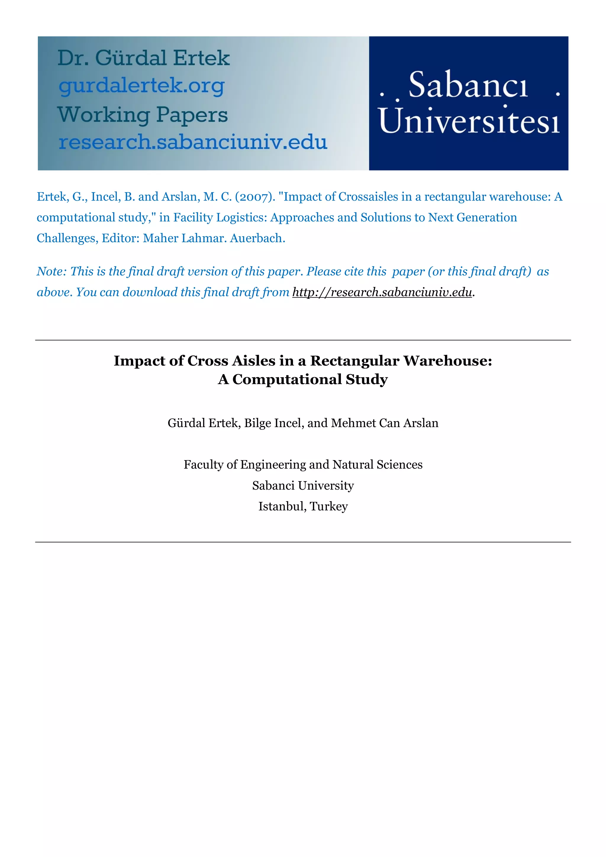
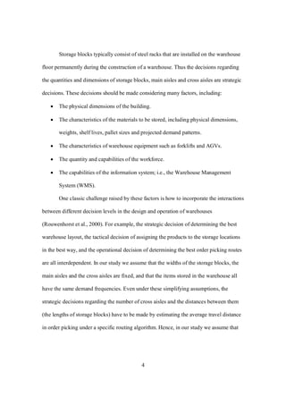
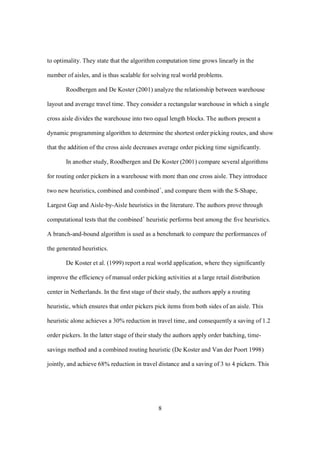
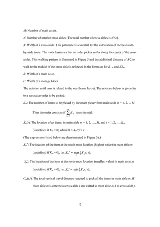
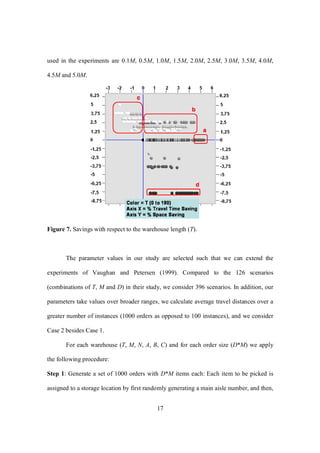
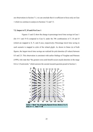
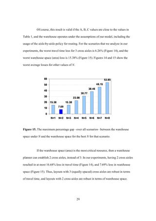
8. Conclusions and Future Work
In this chapter, we presented a detailed discussion of the impact of cross aisles on
a rectangular warehouse. We analyzed both equally spaced and unequally spaced cross
aisles, which we referred to as Case 1 and Case 2, respectively. For Case 1 we utilized the
dynamic programming algorithm presented in Vaughan and Petersen (1999) to determine
the optimal order picking routes under aisle-by-aisle policy. For Case 2, we made
modifications to the Vaughan and Petersen (1999) model, including the change of
formulas for certain parameters and introduction of new expressions before running the
dynamic programming algorithm. We computed the average travel times using Monte
Carlo simulation for 396 distinct scenarios, which correspond to 396 different warehouse
and demand combinations. Our primary findings are:
1. It is more desirable to establish only equally-spaced cross aisles than to establish
unequally spaced cross aisles.
2. Establishing (equally spaced) cross aisles can bring significant travel time savings
and should definitely be considered: We obtained savings up to 35.30% in our
experiments. Biggest travel time savings are realized for pick densities between
0.5 and 2.5 (D[0.5, 2.5]).
3. Given the length of main aisles and the number of main aisles (T and M),
warehouse planners can refer to Table 2 in this chapter to determine the best
number of (equally spaced) cross aisles. If one does not wish to refer to this table,
but wishes to learn and remember a single value for the best number of cross
aisles, we propose the value of 3.

31
There are several directions for future research relating to our study. Below we list
two:
1. It is necessary to design faster and better algorithms to identify the best storage
block lengths (Li) in Case 2, and to validate further our first conclusion.
2. It is important to test the robustness of our conclusions under other demand
patterns and different routing heuristics.
Our study contributes to the research and practice of warehouse planning / facility
logistics by providing actionable insights regarding cross aisles. There is a great potential
for research that attempts to solve warehousing problems that require taking
interdependent decisions at different time horizons; for example at both strategic and
operational levels. Finally, we suggest the adoption of data analysis techniques from the
field of information visualization for discovering knowledge hidden in experimental and
empirical data related to warehouse planning.
Acknowledgements
The authors thank Kemal Kılıç at Sabancı University for his extensive help in reviewing
the M.S. thesis of Bilge Incel (Küçük), which in time turned into this chapter. The
authors also thank Ş. İlker Birbil for reviewing the final draft of the paper and suggesting
many improvements.

32
References
De Koster, R., Roodbergen, K. J., Van Voorden, R. (1999) “Reduction of walking time in
the distribution center of De Bijenkorf,” in New Trends in Distribution Logistics,
M. Grazia Speranza, Paul Stähly, Eds., Springer-Verlag Berlin Heidelberg.
De Koster, R., Van der Poort, E. (1998) “Routing order pickers in a warehouse: a
comparison between optimal and heuristic solutions,” IIE Transactions, vol: 30,
pp. 469-480.
Hoffman, P. E., Grinstein, G. G. (2002) “A survey of visualiations for high-dimensional
data mining,” in Information Visualization in Data Mining and Knowledge
Discovery, Usama Fayyad, Georges Grinstein and Andreas Wierse, Eds., Morgan
Kaufmann.
Frazelle, E. H. (2001) World-class warehousing and material handling. McGraw-Hill.
Frazelle, E. H., Apple, J. M. (1994) “Warehouse operations,” in The Distribution
Management Handbook. James A. Tompkins and Dale Harmelink, Eds. Mc-
Graw-Hill.
Keim, D. A. (2002) “Information visualization and visual data mining,” IEEE
Transactions on Visualization and Computer Graphics, vol: 8 no: 1, pp.1–8
Petersen, C.G. (1997) “An evaluation of order picking routing policies,” International
Journal of Operations and Production Management, vol: 17, pp. 1098-1111.
Ratliff, H. D., Rosenthal, A. S. (1983) “Order Picking in a rectangular warehouse: A
solvable case of the traveling salesman problem,” Operations Research, vol: 31,
no: 3, pp. 507-521.

33
Roodbergen, K. J., De Koster, R. (2001a) “Routing order pickers in a warehouse with a
middle aisle,” European Journal Of Operational Research, vol: 133, pp. 32-33.
Roodbergen, K. J., De Koster, R. (2001b) “Routing methods for warehouses with
multiple cross aisles,” International Journal of Production Research, vol: 39, pp.
1865-1883.
Rouwenhorst, B., Reuter B., Stockrahm, V., Van Houtum, G. J., Mantel, R. J., Zijm, W.
H. M. (2000) “Warehouse design and control: framework and literature review,”
European Journal of Operational Research, vol: 122, pp. 515-533.
Sharp, P.G. (2000) “Warehouse management,” Chapter 81 in Handbook of Industrial
Engineering, Gavriel Salvendy, Ed., John Wiley & Sons, Inc., New York.
Shneiderman, B. (1999) “Dynamic queries, starfield displays, and the path to Spotfire”.
Available under http://www.cs.umd.edu/hcil/spotfire/ . Retrieved on November
2006.
Spence, R. (2001) Information visualization. Essex, England: ACM Press.
Van den Berg, J. P., Zijm, W. H. M. (1999) “Models for warehouse management:
classification and examples,” International Journal of Production Economics,
vol: 59, pp. 519-528.
Vaughan, T. S., Petersen, C. G. (1999) “The effect of warehouse cross aisles on order
picking efficiency,” International Journal of Production Research, vol: 37, pp.
881-897.

34
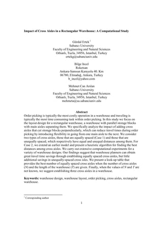
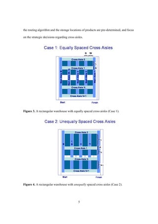
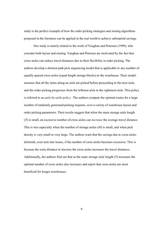
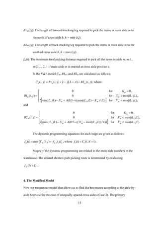
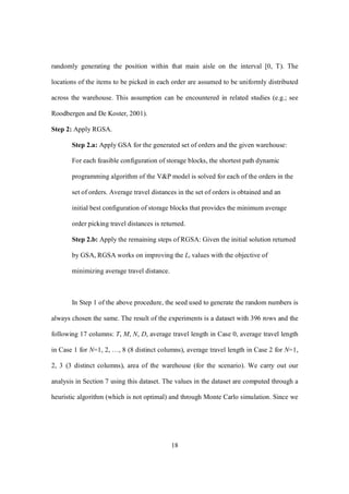
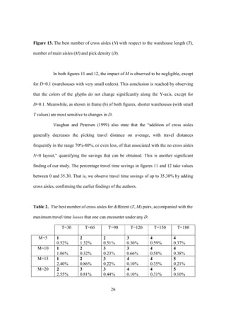
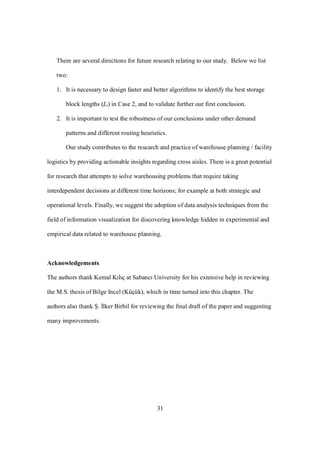
Appendix
GRID_SEARCH_ALGORITHM (GSA)
This algorithm returns bestL, the best block lengths among tested layouts, for a
given N. The length of the gridForL array is (N+1) and indicates the number of storage
blocks. gridsForL[i] records the number of grids that constitute the length of the ith
storage block. If the summation of the elements of gridForL array is equal to noOfGrids
value, then a feasible storage block length combination is obtained. When noOfGrids =
20 and N = 2, for example, then some of the feasible storage block lengths (L1, L2, L3)
would be (1, 12, 7), (11, 4, 5), having the summation of L values equal to noOfGrids =
20.
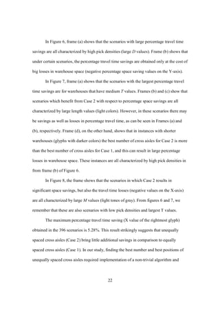
GSA generates feasible configurations of storage blocks systematically and
returns the travel distances by solving the modified model that we present for a uniformly
distributed set of orders. Average of the travel distances for the order set is taken and the
initial best configuration of storage blocks enabling the minimum average order picking
travel distances is labeled as bestL.
This algorithm generates a greater number of feasible storage block length
alternatives as the number of grids is increased. This results in smaller unit length (G=
T/noOfGrids). However, the more the number of feasible solution gets, the more will be
the computational effort. We observed in our experiments that for the warehouse and
order settings described in the next section, noOfGrids = 7 is computationally prohibitive
(18 days running time including the cases where N = 4), and noOfGrids is selected as
seven.

35
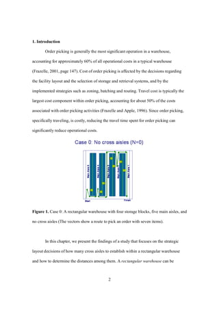
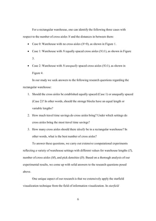
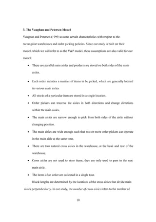
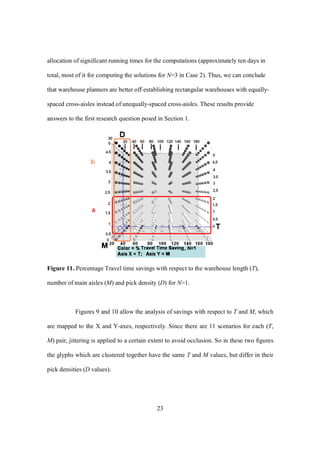
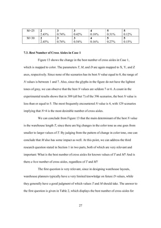
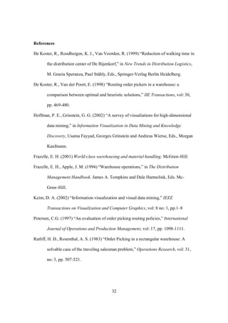
 = {1,...., N+1}, O = {1,...., }
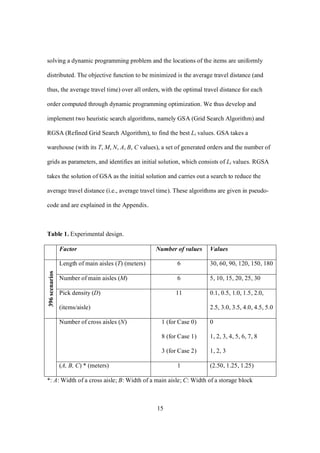
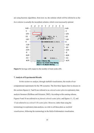
GRID_SEARCH_ALGORITHM (warehouse, orders, noOfGrids)
G = T/noOfGrids
for each gridsForL, /* s.t. gridsForL[i]  noOfGrids, i */
sumOfGrids =
i
 gridsForL[i]
if( sumOfGrids = = noOfGrids&&ARRAY_CONTAINS_NOZERO(gridsForL))
tempL[i] = gridsForL[i] * G, i  
TempWarehouse.setL(tempL)
orders[o].setWarehouse(tempWarehouse), o  O
tempSimulationStatistics = CALCULATE_SIMULATION_STATISTICS(orders)
tempTravelDistance = tempSimulationStatistics.getAverage()
if (tempTravelDistance < bestTravelDistance)
bestL = tempL
bestTravelDistance = tempTravelDistance
return bestL
CALCULATE_SIMULATION_STATISTICS (orders)
travelDistance[o] = getOptimalTravelDistance( orders[o] ), o  O
return statistics for travelDistance data
...........

36
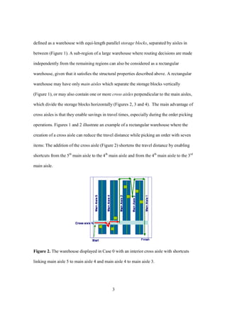
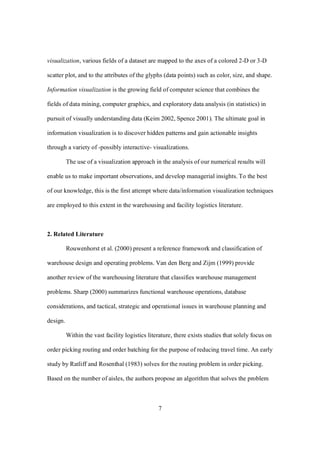
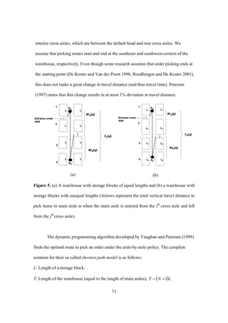
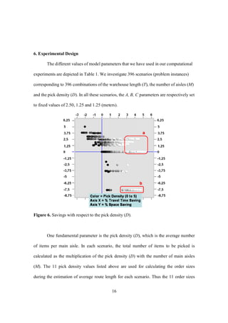
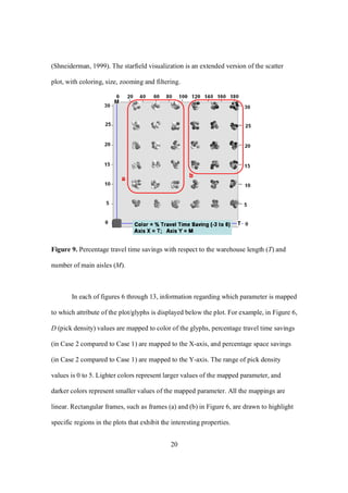
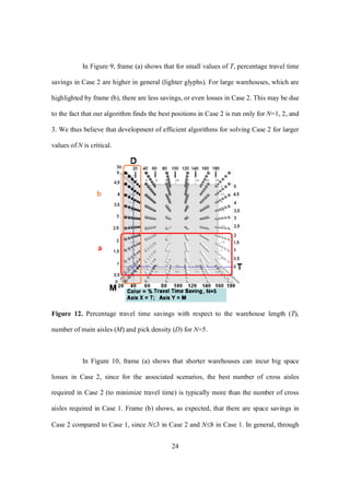
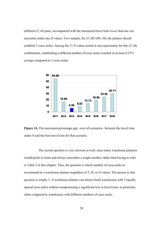
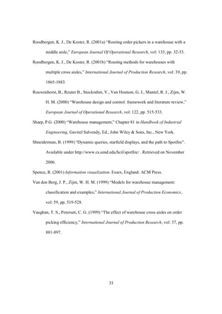
REFINED_GRID_SEARCH_ALGORITHM (RGSA)
This algorithm starts with the result of the grid search algorithm as the initial
solution and applies changes in little unit lengths (G) to the initial best configuration of
storage blocks (initialBestL). In this method, first a range is defined. Half of this range
is subtracted from each storage space length and smaller unit lengths (gridsForL[i]*G)
are added to each storage space length. The travel distance for the new configuration
tempL is calculated for the given order set (orders) and compared with the best result
obtained until that time. After trying all feasible configurations of the gridsForL for the
same initial solution and calculating the travel distance for the new storage block lengths,
tempL resulting in the shortest travel distance is assigned as the best configuration of
cross aisles, bestL. Then the range is updated by dividing with the number of grids
(noOfGrids). Half of this range is subtracted from each storage space length and smaller
unit lengths (gridsForL[i]*G) are added to obtain new feasible storage block lengths
(tempL) and travel distance implied by the updated tempL is calculated for the given
order set (orders). The refined grid search is continued until the range declines to a
length, which is determined as the smallest range (resolution) to be considered. When the
range becomes as small as the resolution, the refined grid search is terminated and the
improved configuration of storage block lengths is assigned as the best configuration of
storage block lengths (bestL) for the given warehouse and order set.
Any element of gridsForL can be at most (N+1)*noOfGrids, because in the
refined grid search algorithm for each storage block, half of the range is subtracted and
the length gridsForL[i]*G is added, for instance:
From the above equations it is clearly seen that summation of the gridsForL’s

37
elements has to be (N+1)*noOfGrids. Therefore, an element of gridsForL is allowed to be
(N+1)*noOfGrids at most.
The search algorithms result in the best storage block lengths that give the
minimum order picking travel distance for a problem instance (T, M, N, A, B, C, D)
among the tested configurations.
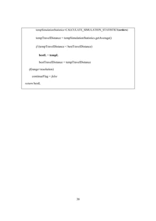
REFINED_GRID_SEARCH_ALGORITHM(warehouse, orders, noOfGrids, resolution)
initialBestL = GRID_SEARCH_ALGORITHM(warehouse, orders, noOfGrids)
range = T/noOfGrids
iterationNo = 0
continueFlag = true
while (continueFlag)
iterationNo++
if (iterationNo > 1) // if not the first iteration
range = (range/noOfGrids)/2
G = (range/noOfGrids)/2
for each gridsForL /* gridsForL[i]  (N+1)*noOfGrids */
sumOfGrids =
i
 gridsForL[i]
if (sumOfGrids==(N+1)noOfGrids&&ARRAY_CONTAINS_NOZERO(gridsForL))
tempL[i] = initialBestL[i] – (range/2) + gridsForL[i]*G, i  
tempWarehouse.setL(tempL)
orders[o].setWarehouse(tempWaarehouse), o  O

38
tempSimulationStatistics=CALCULATE_SIMULATION_STATISTICS(orders)
tempTravelDistance = tempSimulationStatistics.getAverage()
if (tempTravelDistance < bestTravelDistance)
bestL = tempL
bestTravelDistance = tempTravelDistance
if(range<resolution)
continueFlag = false
return bestL

Impact of Cross Aisles in a Rectangular Warehouse:A Computational Study

Recommended

Recommended

More Related Content

Similar to Impact of Cross Aisles in a Rectangular Warehouse:A Computational Study

Similar to Impact of Cross Aisles in a Rectangular Warehouse:A Computational Study (20)

More from Gurdal Ertek

More from Gurdal Ertek (20)

Recently uploaded

Recently uploaded (20)

Impact of Cross Aisles in a Rectangular Warehouse:A Computational Study