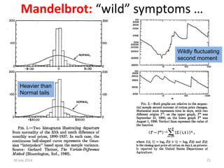
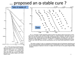
Downloaded 10 times
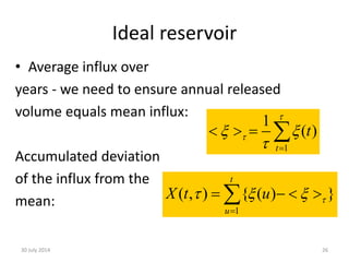
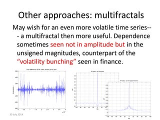
![Persistence & heat waves
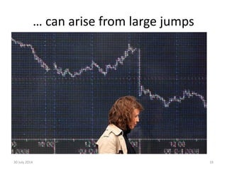
• Rather than coming from a fat-tailed
distribution of amplitudes, the severity of an
event might be a result of a long duration.
• Runs of hot days above a fixed threshold, e.g.
summer 1976 in UK, or summer 2003 in
France.
• Direct link to weather
derivatives [e.g. book
by Steve Jewson et al]](https://image.slidesharecdn.com/ima2013-140730004936-phpapp01/85/IMA-2013-Bunched-Black-Swans-at-the-British-Antarctic-Survey-7-320.jpg)
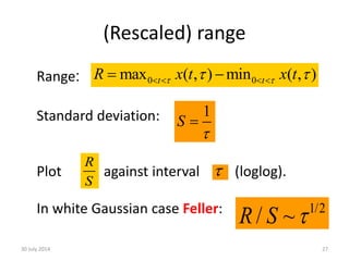
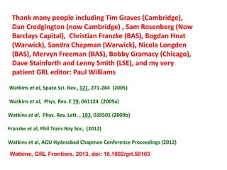
![Finance: persistence & fat tails ?
“ “We were seeing things that were 25-standard deviation
moves, several days in a row,” said David Viniar,
Goldman’s CFO ... [describing catastrophic losses on their
flagship Global Alpha hedge fund]. “What we have to look
at more closely is the phenomenon of the crowded trade
overwhelming market
fundamentals”,
he said. “It makes
you reassess how
big the extreme
moves can be””.
--- FT, August 13th, 2007](https://image.slidesharecdn.com/ima2013-140730004936-phpapp01/85/IMA-2013-Bunched-Black-Swans-at-the-British-Antarctic-Survey-8-320.jpg)
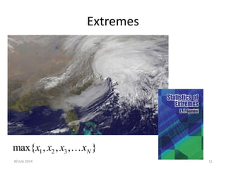
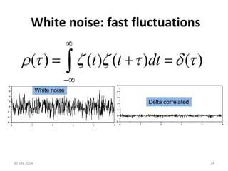
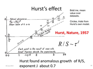
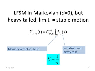
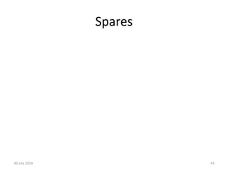
![Bursts
30 July 2014 12
2
1
[ ( ') ] '
t
t
s x t L dt 2
1
'
t
t
T dt
Inspired by sandpiles
and SOC.
Compared, for
example to EVT,
does not assume
threshold is in some
sense high.
Can be measured on
time series, or fields,
has links to research on
sojourns, level sets,
etc.](https://image.slidesharecdn.com/ima2013-140730004936-phpapp01/85/IMA-2013-Bunched-Black-Swans-at-the-British-Antarctic-Survey-12-320.jpg)
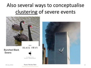
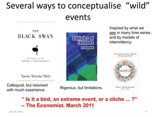
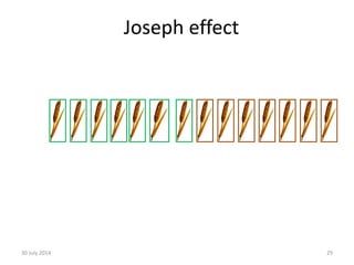
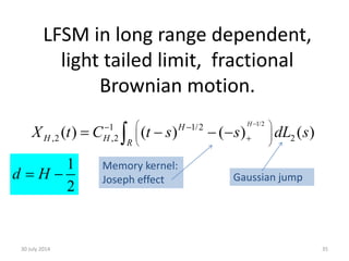
![Several ways to think about
dependent“wild” events
• If considering extreme values, the largest (or
smallest) of a set, and can use, or infer, a model, then
EV theory [e.g. Gumbel; Coles] is mature … & is now
developed to encompass clustering.
• Rather than EVT, however, today concerned with
burst framework (“grouped grey swans”) .
• Why is burst a different concept, and what kind of
“routinely extreme” randomness does it represent ?
• And why do I use the phrase “routinely extreme”
30 July 2014 14](https://image.slidesharecdn.com/ima2013-140730004936-phpapp01/85/IMA-2013-Bunched-Black-Swans-at-the-British-Antarctic-Survey-14-320.jpg)
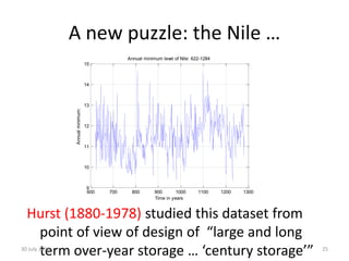
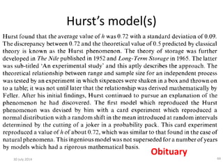
![Grey swans: “routinely extreme”
• In The Black Swan, Taleb observes that “Extremistan does not
always imply Black Swans. Some events can [be]... somewhat
predictable [ ...]. They are near–Black Swans ... I call this
special case of “gray” swans Mandelbrotian randomness”.
30 July 2014 15
600 700 800 900 1000 1100 1200 1300
9
10
11
12
13
14
15
Annual minimum level of Nile: 622-1284
Annualminimum:
Time in years
As John Prescott put it (and was widely mocked) :
“Extreme events will be the norm”](https://image.slidesharecdn.com/ima2013-140730004936-phpapp01/85/IMA-2013-Bunched-Black-Swans-at-the-British-Antarctic-Survey-15-320.jpg)
![Grey swans: “routinely extreme”
• In The Black Swan, Taleb observes that “Extremistan does not
always imply Black Swans. Some events can [be]... somewhat
predictable [ ...]. They are near–Black Swans ... I call this
special case of “gray” swans Mandelbrotian randomness”.
30 July 2014 16
600 700 800 900 1000 1100 1200 1300
9
10
11
12
13
14
15
Annual minimum level of Nile: 622-1284
Annualminimum:
Time in years
Or as JP might have put it:
“Extremely large &/or long-lived
events will be commonplace”](https://image.slidesharecdn.com/ima2013-140730004936-phpapp01/85/IMA-2013-Bunched-Black-Swans-at-the-British-Antarctic-Survey-16-320.jpg)
![Gaussian (normal): “mild” variation
30 July 2014 17
21
exp{ (1/ 2)[( ) / ]) }
2
(p
If we want to model
positive rvs an exponential
gives light tails, for example.](https://image.slidesharecdn.com/ima2013-140730004936-phpapp01/85/IMA-2013-Bunched-Black-Swans-at-the-British-Antarctic-Survey-17-320.jpg)
![30 July 2014
18
Light tail
Heavy tail
Tails may be not just fat however,
but (rigorously) heavy …
Pareto distribution is one such
( ) ( )
x
F x p d df
( ) 1 ( ) 0,F x F x x Tail of
df
0
( ) ,
1
( ) 0I
x
F y dx xF y
Integrated tail of df
Example, tail of Pareto distribution makes the integral
in the Cramer-Lundberg condition diverge:
0 0
( ) (1 )x x
e x dxF e x dx
Essential distinction of small & large
claim distributions [Embrechts et al book]](https://image.slidesharecdn.com/ima2013-140730004936-phpapp01/85/IMA-2013-Bunched-Black-Swans-at-the-British-Antarctic-Survey-18-320.jpg)
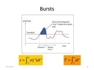
![Auroral physics: fat tails
pdf of AE
Magnetometer time series
AU
AL
AE=AU-AL
Hnat et al, NPG [2004]
S&P 500
Mantegna & Stanley](https://image.slidesharecdn.com/ima2013-140730004936-phpapp01/85/IMA-2013-Bunched-Black-Swans-at-the-British-Antarctic-Survey-23-320.jpg)
![log s
log
P(T)
log
P()
logT
log
Poynting flux in solar wind plasma from NASA
Wind Spacecraft at Earth-Sun L1 point
Freeman, Watkins & Riley [PRE, 2000].
log
P(s) size
length
waiting time
some bursts we made earlier
Data](https://image.slidesharecdn.com/ima2013-140730004936-phpapp01/85/IMA-2013-Bunched-Black-Swans-at-the-British-Antarctic-Survey-37-320.jpg)
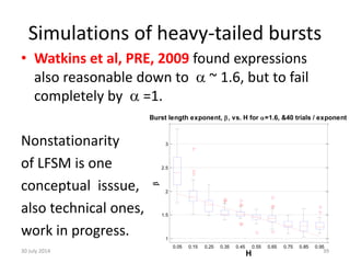
![Simulations of light-tailed bursts
• Power laws for pdf of burst size s, and duration T
predicted to have exponents =-2/(1+H) & =2-H
respectively [Watkins et al, Phys. Rev. E, 2009 ].
• Good agreement in Gaussian (fBm) limit: Confirmed
findings of Carbone et al [PRE, 2004] & Rypdal and
Rypdal [PRE, 2008].
30 July 2014 38
=-2/(1+H) =2-H
gamma
H H
beta](https://image.slidesharecdn.com/ima2013-140730004936-phpapp01/85/IMA-2013-Bunched-Black-Swans-at-the-British-Antarctic-Survey-38-320.jpg)
![Recap
• Some natural severe events may be rare extremes, tractable with EVT
[e.g. Coles, 2001], adapted to allow correlation if present.
• Others may belong to a different class [studied by Mandelbrot] “Bursty”
time series may show comparatively frequent high amplitude events,
and/or long range correlations between successive values. The frequent
large values due to the first of these effects can give rise to an burst
composed of successive wild events. Conversely, long range dependence,
even in a light-tailed Gaussian model, can integrate ``mild” events into a
extreme burst
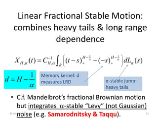
• I showed a standard statistical time series model, linear fractional stable
motion (LFSM), which allows these two effects to be varied independently.
Presented results from a preliminary study of such bursts [Watkins et al,
PRE, 2009].
• Other options for burst scaling modelling including multiplicative cascades
(such as multifractals).
41](https://image.slidesharecdn.com/ima2013-140730004936-phpapp01/85/IMA-2013-Bunched-Black-Swans-at-the-British-Antarctic-Survey-41-320.jpg)

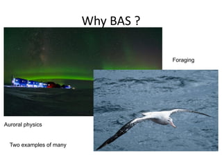
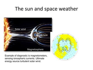
- THE WHAT: The speaker will discuss "bunched black swans", which are long range correlated, wild events. Specifically, the speaker will discuss "bursts" where the time series exceeds a threshold. - THE WHY: Scientists studying climate, space weather, and finance care about bursts. The speaker will provide examples of why this is relevant to the British Antarctic Survey (BAS) and beyond. - THE HOW: The speaker will discuss how they have modeled one class of "routinely extreme" burst problems using an approach building on Mandelbrot's work, involving fractional stable models.


