UNIT 4 MEASURES OF SKEWNESS AND
KURTOSIS
Structure
4.0 Objectives
4.1 Introduction
4.2 Concept of Skewness
4.2.1 Karl Pearson's Measure of Skewness
4.2.2 Bowley's Measure of Skewness
4.2.3 Kelly's Measure of Skewness
4.3 Moments
4.4 Concept and Measure of Kurtosis
4.5 Let Us Sum Up
4.6 Answers or Hints to Check Your Progress Exercises
4.0 OBJECTIVES
After going through this Unit, you will be able to:
 distinguish between a symmetrical and a skewed distribution;
 compute various coefficients to measure the extent o f skewness in a
distribution;
 distinguish between platykurtic, mesokurtic and leptokurtic distributions
and
 compute the coefficient of kurtosis.
4.1 INTRODUCTION
In this unit you will learn various techniques to distinguish between various
shapes of a frequency distribution. This is the final unit with regard to the
summarization of univariate data. This unit will make you familiar with the
concept of skewness and kurtosis. The need to study these concepts arises from
the fact that the measures of central tendency and dispersion fail to describe a
distribution completely. It is possible to have frequency distributions which differ
widely in their nature and composition and yet may have same central tendency
and dispersion. Thus, there is need to supplement the measures of central
tendency and dispersion. Consequently, in this unit, we shall discuss two such
measures, viz., measures of skewness and kurtosis.

Adapted from IGNOU study material of EEC 13: Elementary Statistical Methods and Survey Techniques,
Units 4, 5 and 6 written by R S Bharadwaj with modifications by Kaustuva Barik
85
Measures of Skewness
and Kurtosis
4.2 CONCEPT OF SKEWNESS
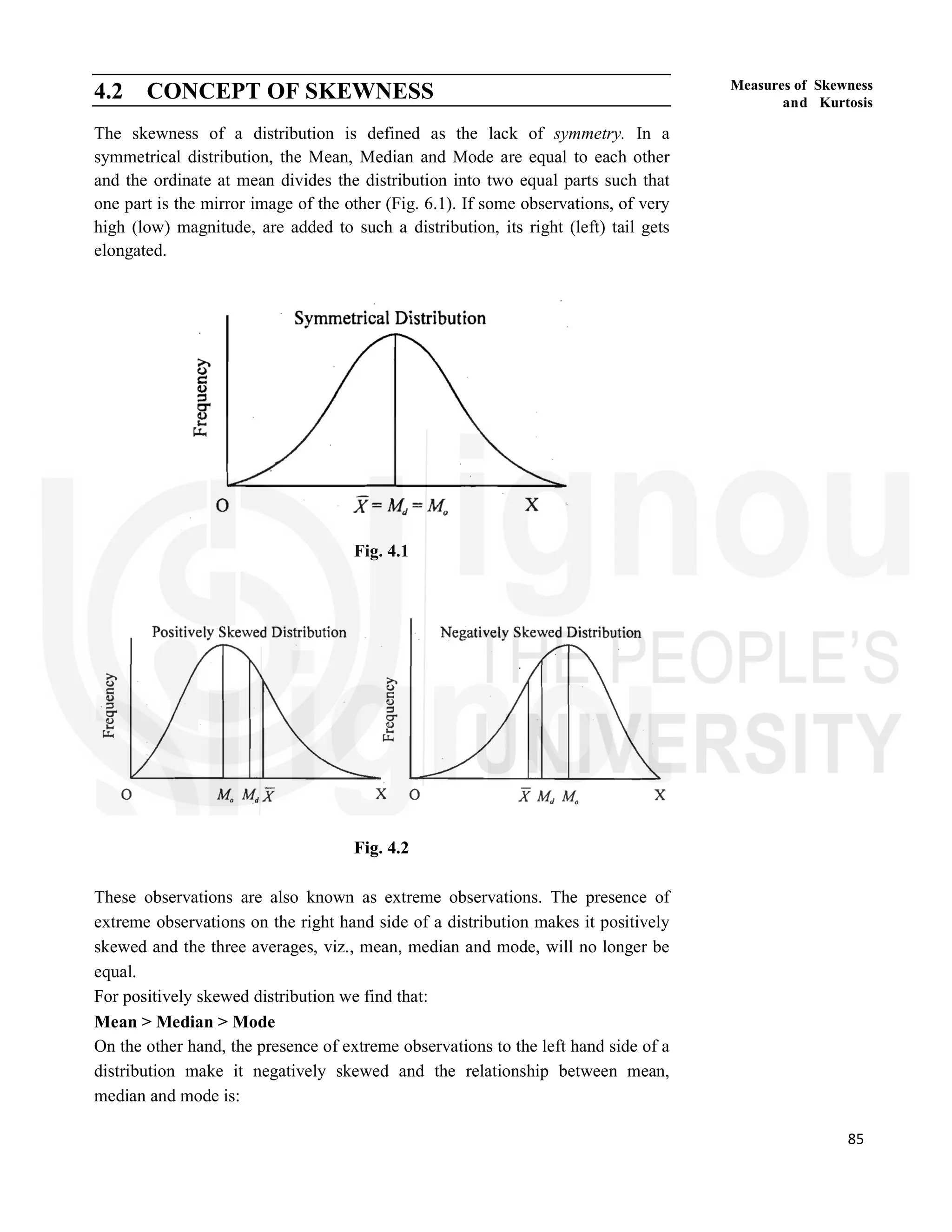
The skewness of a distribution is defined as the lack of symmetry. In a
symmetrical distribution, the Mean, Median and Mode are equal to each other
and the ordinate at mean divides the distribution into two equal parts such that
one part is the mirror image of the other (Fig. 6.1). If some observations, of very
high (low) magnitude, are added to such a distribution, its right (left) tail gets
elongated.
Fig. 4.1
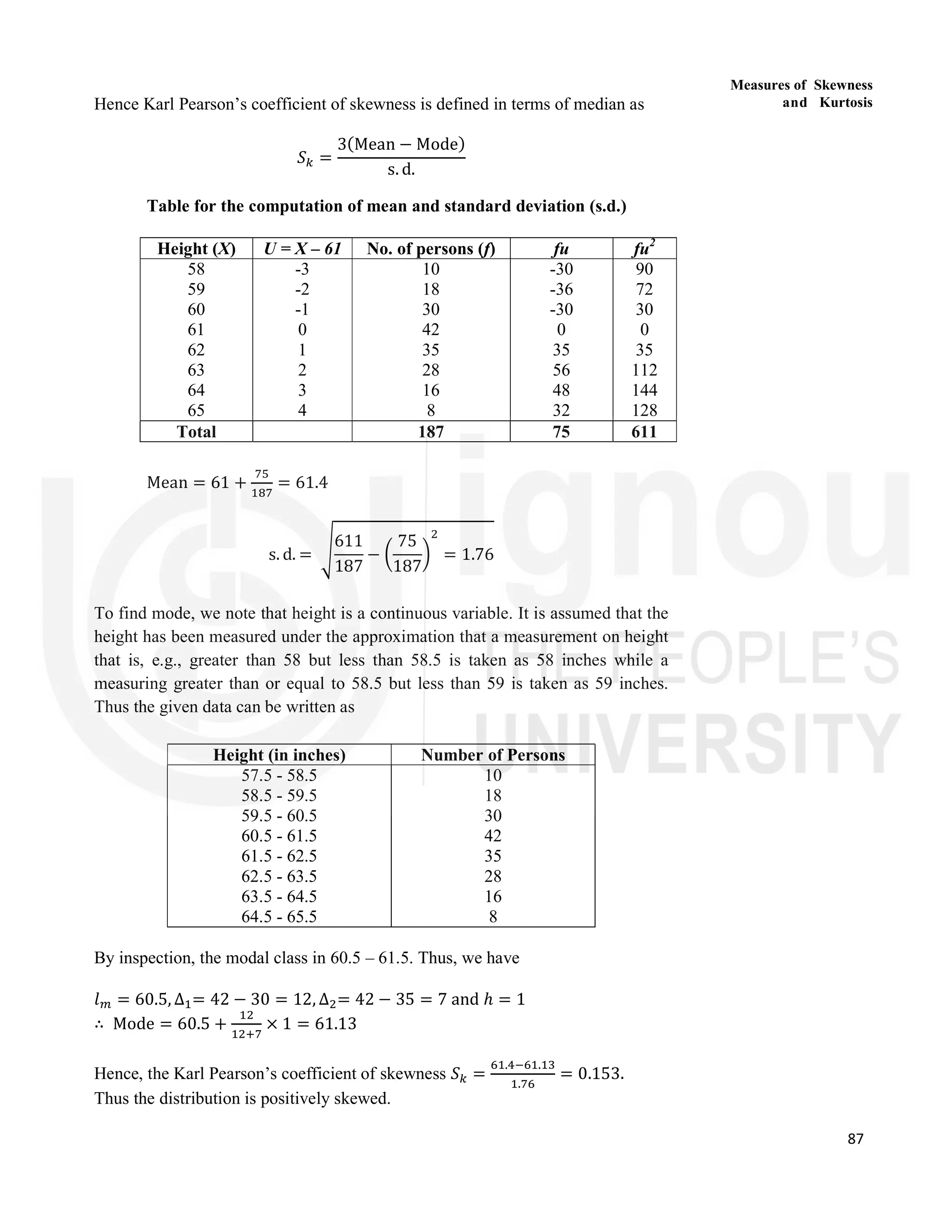
Fig. 4.2
These observations are also known as extreme observations. The presence of
extreme observations on the right hand side of a distribution makes it positively
skewed and the three averages, viz., mean, median and mode, will no longer be
equal.
For positively skewed distribution we find that:
Mean > Median > Mode
On the other hand, the presence of extreme observations to the left hand side of a
distribution make it negatively skewed and the relationship between mean,
median and mode is:
86
Descriptive
Statistics
Mean < Median < Mode
In Fig. 4.2 we depict the shapes of positively skewed and negatively skewed
distributions. The direction and extent of skewness can be measured in various
ways. We will discuss four measures of skewness in this unit.
4.2.1 Karl Pearson’s Measure of Skewness
In Fig. 4.2 you noticed that the mean, median and mode are not equal in a skewed
distribution. The Karl Pearson’s measure of skewness is based upon the
divergence of mean from mode in a skewed distribution.
Since Mean = Mode in a symmetrical distribution, (Mean – Mode) can be taken
as an absolute measure of skewnes. The absolute measure of skewness for a
distribution depends upon the unit of measurement. For example, if the mean =
2.45 metre and mode = 2.14 metre, then absolute measure of skewness will be
2.45 metre – 2.14 metre = 0.31 metre. For the same distribution, if we change the
unit of measurement to centimeters, the absolute measure of skewness is 245
centimetre – 214 centimetre = 31 centimatre. In order to avoid such a problem
Karl Pearson takes a relative measure of skewness.
A relative measure, independent of the units of measurement, is defined as the
Karl Pearson’s Coefficient of skewness Sk, given by
𝑆 =
Mean − Mode
s. d.
The sign of 𝑆 gives the direction and its magnitude gives the extent of skewness.
If 𝑆 > 0, the distribution is positively skewed, and if 𝑆 < 0 it is negatively
skewed.
Example 4.1: Compute the Karl Pearson’s coefficient of skewness from the
following data:
Height (in inches) Number of Persons
58
59
60
61
62
63
64
65
10
18
30
42
35
28
16
8
So far we have seen that 𝑆 is strategically dependent upon mode. If mode is not
defined for a distribution we cannot find 𝑆 . The empirical relation between
mean, median and mode states that, for a moderately symmetrical distribution,
we have median and mode states that, for a moderately symmetrical distribution,
we have
Mean – Mode ≈3 (Mean – Median)
87
Measures of Skewness
and Kurtosis
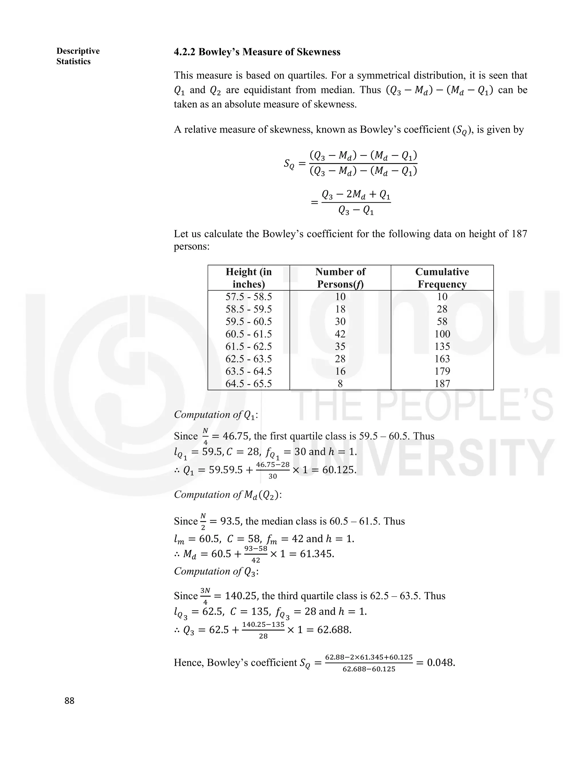
Hence Karl Pearson’s coefficient of skewness is defined in terms of median as
𝑆 =
3(Mean − Mode)
s. d.
Table for the computation of mean and standard deviation (s.d.)
Height (X) U = X – 61 No. of persons (f) fu fu2
58
59
60
61
62
63
64
65
-3
-2
-1
0
1
2
3
4
10
18
30
42
35
28
16
8
-30
-36
-30
0
35
56
48
32
90
72
30
0
35
112
144
128
Total 187 75 611
Mean = 61 + = 61.4
s. d. =
611
187
−
75
187
= 1.76
To find mode, we note that height is a continuous variable. It is assumed that the
height has been measured under the approximation that a measurement on height
that is, e.g., greater than 58 but less than 58.5 is taken as 58 inches while a
measuring greater than or equal to 58.5 but less than 59 is taken as 59 inches.
Thus the given data can be written as
Height (in inches) Number of Persons
57.5 - 58.5
58.5 - 59.5
59.5 - 60.5
60.5 - 61.5
61.5 - 62.5
62.5 - 63.5
63.5 - 64.5
64.5 - 65.5
10
18
30
42
35
28
16
8
By inspection, the modal class in 60.5 – 61.5. Thus, we have
𝑙 = 60.5, ∆ = 42 − 30 = 12, ∆ = 42 − 35 = 7 and ℎ = 1
∴ Mode = 60.5 + × 1 = 61.13
Hence, the Karl Pearson’s coefficient of skewness 𝑆 =
. .
.
= 0.153.
Thus the distribution is positively skewed.
88
Descriptive
Statistics
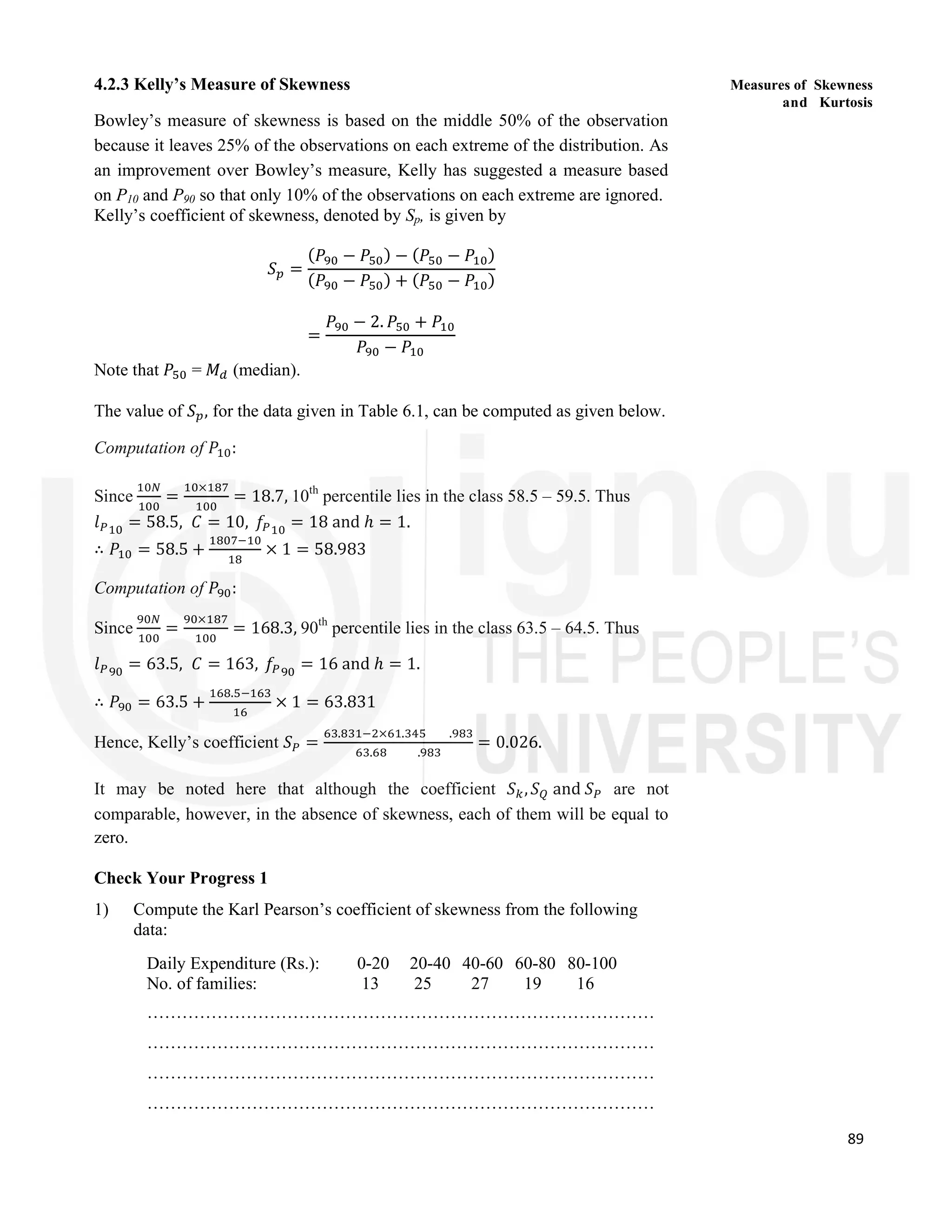
4.2.2 Bowley’s Measure of Skewness
This measure is based on quartiles. For a symmetrical distribution, it is seen that
𝑄 and 𝑄 are equidistant from median. Thus (𝑄 − 𝑀 ) − (𝑀 − 𝑄 ) can be
taken as an absolute measure of skewness.
A relative measure of skewness, known as Bowley’s coefficient (𝑆 ), is given by
𝑆 =
(𝑄 − 𝑀 ) − (𝑀 − 𝑄 )
(𝑄 − 𝑀 ) − (𝑀 − 𝑄 )
=
𝑄 − 2𝑀 + 𝑄
𝑄 − 𝑄
Let us calculate the Bowley’s coefficient for the following data on height of 187
persons:
Height (in
inches)
Number of
Persons(f)
Cumulative
Frequency
57.5 - 58.5
58.5 - 59.5
59.5 - 60.5
60.5 - 61.5
61.5 - 62.5
62.5 - 63.5
63.5 - 64.5
64.5 - 65.5
10
18
30
42
35
28
16
8
10
28
58
100
135
163
179
187
Computation of 𝑄 :
Since = 46.75, the first quartile class is 59.5 – 60.5. Thus
𝑙 = 59.5, 𝐶 = 28, 𝑓 = 30 and ℎ = 1.
∴ 𝑄 = 59.59.5 +
.
× 1 = 60.125.
Computation of 𝑀 (𝑄 ):
Since = 93.5, the median class is 60.5 – 61.5. Thus
𝑙 = 60.5, 𝐶 = 58, 𝑓 = 42 and ℎ = 1.
∴ 𝑀 = 60.5 + × 1 = 61.345.
Computation of 𝑄 :
Since = 140.25, the third quartile class is 62.5 – 63.5. Thus
𝑙 = 62.5, 𝐶 = 135, 𝑓 = 28 and ℎ = 1.
∴ 𝑄 = 62.5 +
.
× 1 = 62.688.
Hence, Bowley’s coefficient 𝑆 =
. × . .
. .
= 0.048.
89
Measures of Skewness
and Kurtosis
4.2.3 Kelly’s Measure of Skewness
Bowley’s measure of skewness is based on the middle 50% of the observation
because it leaves 25% of the observations on each extreme of the distribution. As
an improvement over Bowley’s measure, Kelly has suggested a measure based
on P10 and P90 so that only 10% of the observations on each extreme are ignored.
Kelly’s coefficient of skewness, denoted by Sp, is given by
𝑆 =
(𝑃 − 𝑃 ) − (𝑃 − 𝑃 )
(𝑃 − 𝑃 ) + (𝑃 − 𝑃 )
=
𝑃 − 2. 𝑃 + 𝑃
𝑃 − 𝑃
Note that 𝑃 = 𝑀 (median).
The value of 𝑆 , for the data given in Table 6.1, can be computed as given below.
Computation of 𝑃 :
Since =
×
= 18.7, 10th
percentile lies in the class 58.5 – 59.5. Thus
𝑙 = 58.5, 𝐶 = 10, 𝑓 = 18 and ℎ = 1.
∴ 𝑃 = 58.5 + × 1 = 58.983
Computation of 𝑃 :
Since =
×
= 168.3, 90th
percentile lies in the class 63.5 – 64.5. Thus
𝑙 = 63.5, 𝐶 = 163, 𝑓 = 16 and ℎ = 1.
∴ 𝑃 = 63.5 +
.
× 1 = 63.831
Hence, Kelly’s coefficient 𝑆 =
. × . .
. .
= 0.026.
It may be noted here that although the coefficient 𝑆 ,𝑆 and 𝑆 are not
comparable, however, in the absence of skewness, each of them will be equal to
zero.
Check Your Progress 1
1) Compute the Karl Pearson’s coefficient of skewness from the following
data:
Daily Expenditure (Rs.): 0-20 20-40 40-60 60-80 80-100
No. of families: 13 25 27 19 16
……………………………………………………………………………
……………………………………………………………………………
……………………………………………………………………………
……………………………………………………………………………
90
Descriptive
Statistics
2) The following figures relate to the size of capital of 285 companies:
Compute the Bowley’s and Kelly’s coefficients of skewness and interpret
the results.
……………………………………………………………………………
……………………………………………………………………………
……………………………………………………………………………
……………………………………………………………………………
3) The following measures were computed for a frequency distribution:
Mean = 50, coefficient of Variation = 35% and Karl Pearson’s Coefficient
of Skewness = ─ 0.25. Compute Standard Deviation, Mode and Median
of the distribution.
……………………………………………………………………………
……………………………………………………………………………
……………………………………………………………………………
……………………………………………………………………………
4.3 MOMENTS
The rth
moment about mean of a distribution, denoted by μ , is given by
μ =
1
𝑁
𝑓 (𝑋 − 𝑋) , where 𝑟 = 0, 1, 2, 3, 4, … … . .
Thus, rth
moment about mean is the mean of the rth
power of deviations of
observations from their arithmetic mean. In particular,
if 𝑟 = 0, we have μ =
1
𝑁
𝑓(𝑋 − 𝑋) = 1,
if 𝑟 = 1, we have μ =
1
𝑁
𝑓(𝑋 − 𝑋) = 0,
if 𝑟 = 2, we have μ =
1
𝑁
𝑓 (𝑋 − 𝑋) = 𝜎 ,
if 𝑟 = 3, we have μ =
1
𝑁
𝑓 (𝑋 − 𝑋) and so on.
These moments are also known as central moments.
In addition to the above, we can define raw moments as moments about any
arbitrary mean.
Capital (in Rs. lacs.) 1-5 6-10 11-15 16-20 21-25 26-30 31-35 Total
No. of companies 20 27 29 38 48 53 70 285
91
Measures of Skewness
and Kurtosis
Let A denote an arbitrary mean, then rth
moment about A is defined as
μ =
1
𝑁
𝑓 (𝑋 − 𝐴) , 𝑟 = 0, 1, 2, 3, … . .
When A = 0, we get various moments about origin.
Moment Measure of Skewness
The moment measure of skewness is based on the property that, for a
symmetrical distribution, all odd ordered central moments are equal to zero. We
note that μ = 0, for every distribution, therefore, the lowest order moment that
can provide an absolute measure of skewness is μ .
Further, a coefficient of skewness, independent of the units of measurement, is
given by
α = = β =
±
γ , where β and γ are defined as the first beta and first
gamma coefficients respectively. Note that β is a measure of kurtosis as you will
come to know in the next Section.
Very often, the skewness is measured in terms of β = , where the sign of
skewness is determined by the sign of μ .
Example 4.2: Compute the Moment coefficient of skewness (β ) from the
following data.
Marks Obtained: 0-10 10-20 20-30 30-40 40-50 50-60 60-70
Frequency: 6 12 22 24 16 12 8
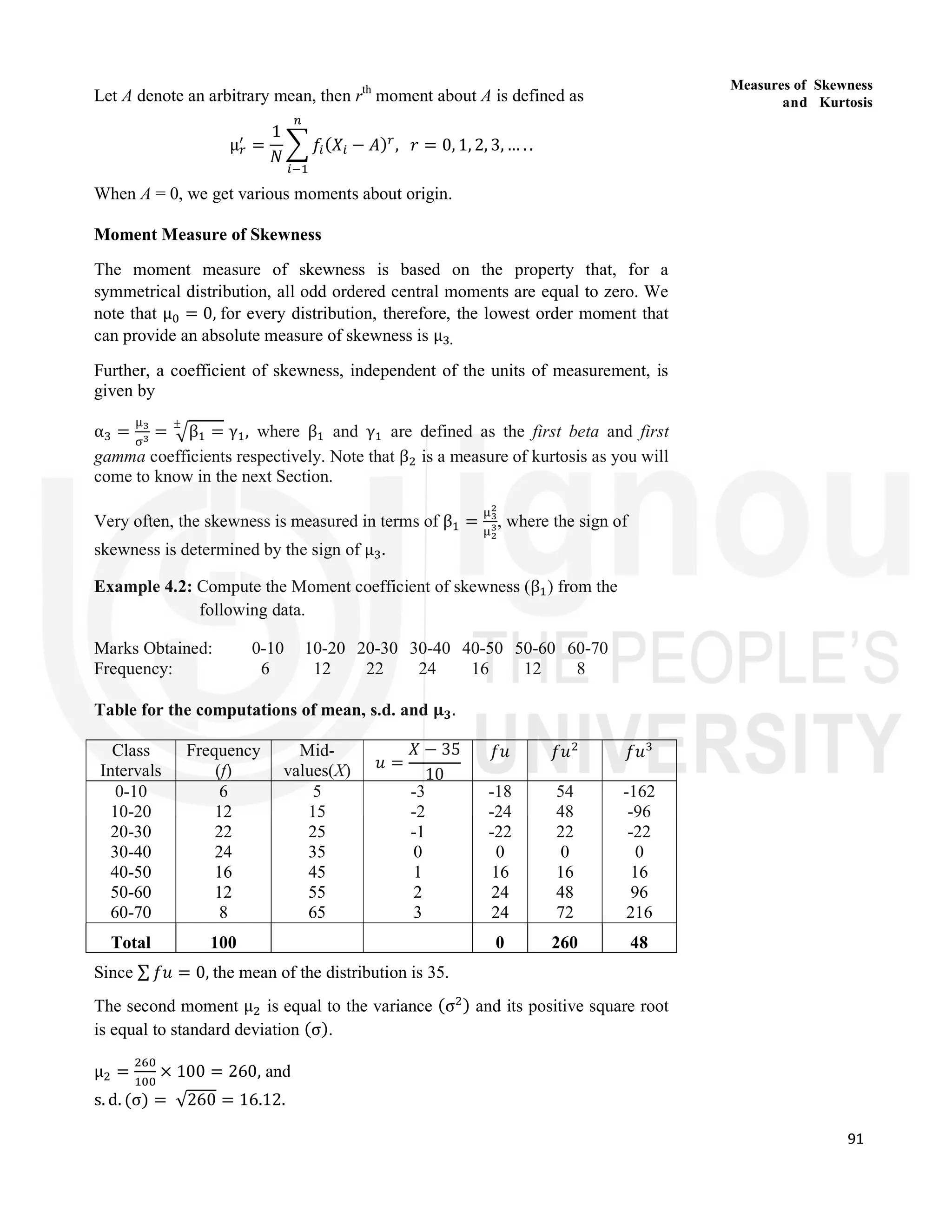
Table for the computations of mean, s.d. and 𝛍𝟑.
Class
Intervals
Frequency
(f)
Mid-
values(X) 𝑢 =
𝑋 − 35
10
𝑓𝑢 𝑓𝑢 𝑓𝑢
0-10
10-20
20-30
30-40
40-50
50-60
60-70
6
12
22
24
16
12
8
5
15
25
35
45
55
65
-3
-2
-1
0
1
2
3
-18
-24
-22
0
16
24
24
54
48
22
0
16
48
72
-162
-96
-22
0
16
96
216
Total 100 0 260 48
Since ∑ 𝑓𝑢 = 0, the mean of the distribution is 35.
The second moment μ is equal to the variance (σ ) and its positive square root
is equal to standard deviation (σ).
μ = × 100 = 260, and
s. d. (σ) = √260 = 16.12.
92
Descriptive
Statistics
Also, μ = × 1000 = 480.
Thus, β =
( )
( )
= 0.01.
Since the sign of 𝜇 is positive and β is small, the distribution is slightly
positively skewed.
If the mean of a distribution is not a convenient figure like 35, as in the above
example, the computation of various central moments may become a
cumbersome task. Alternatively, we can first compute raw moments and then
convert them into central moments by using the equations obtained below.
Conversion of Raw Moments into Central Moments
We can write
μ =
1
𝑁
𝑓 (𝑋 − 𝑋) =
1
𝑁
𝑓 [(𝑋 − 𝐴) − (𝑋 − 𝐴)]
=
1
𝑁
𝑓 [(𝑋 − 𝐴) − μ ] (Sinceμ ==
1
𝑁
𝑓 (𝑋 − 𝐴) = 𝑋 − 𝐴)
Expanding the term within brackets by binomial theorem, we get
=
1
𝑁
𝑓 𝑟∁ (𝑋 − 𝐴) μ − 𝑟∁ (𝑋 − 𝐴) μ + 𝑟∁ (𝑋 − 𝐴) μ − ⋯
=
1
𝑁
𝑓 (𝑋 − 𝐴) − 𝑟∁
1
𝑁
𝑓 (𝑋 − 𝐴) μ + 𝑟∁
+
1
𝑁
𝑓 (𝑋 − 𝐴) μ − ⋯
From the above, we can write
μ = μ − 𝑟∁ μ μ + 𝑟∁ μ μ − 𝑟∁ 𝑟∁ μ μ + ⋯
In particular, taking r = 2, 3, 4, etc., we get
μ = μ − 2∁ μ + 2∁ μ μ = μ − μ (μ = 1)
μ = μ − 3μ μ + 3μ − μ = μ − 3μ μ + 2μ
μ = μ − 4μ μ + 6μ μ − 4μ + μ = μ − 4μ μ + 6μ μ − 3μ
Example 4.3: Compute the first four moments about mean from the
following data.
Class Intervals: 0 – 10 10 – 20 20 – 30 30 – 40
Frequency (f) : 1 3 4 2
Table for computations of raw moments (Take A = 25).
93
Measures of Skewness
and Kurtosis
Class Intervals f Mid-Value 𝑢 = 𝑓𝑢 𝑓𝑢 𝑓𝑢 𝑓𝑢
0 – 10 1 5 – 2 – 2 4 -8 16
10 – 20 2 15 – 1 – 3 3 -3 3
20 – 30 3 25 0 0 0 0 0
30 – 40 4 35 1 2 2 2 2
Total 10 – 3 9 – 9 21
From the above table, we can write
μ =
−3 × 10
10
= −3,
μ =
9 × 10
10
= 90,
μ =
−9 × 10
10
= −900 and
μ =
21 × 10
10
= 2100
Moments about Mean
By definition,
μ = 0,
μ = 90 − 9 = 81,
μ = −900 − 3 × 90 × (−3) + 2 × (−3) = −900 + 810 − 54 = −144 and
μ = 21000 − 4 × (−900) × (−3) + 6 × 90 × (−3) − 3 × (−3)
= 21000 − 10800 + 4860 − 243 = 14817.
Check Your Progress 2
1) Calculate the first four moments about mean for the following
distribution. Also, calculate β and comment upon the nature of skewness.
Class Intervals: 0 – 20 20 – 40 40 – 60 60 – 80 80 – 100
Frequency (f) : 8 28 35 17 12
……………………………………………………………………………
……………………………………………………………………………
……………………………………………………………………………
……………………………………………………………………………
94
Descriptive
Statistics
2) The first three moment of distribution about the value 3 of a variable are
2, 10 and 30 respectively. Obtain 𝑋, 𝜇 , 𝜇 and hence 𝛽 . Comment upon
the nature of skewness.
……………………………………………………………………………
……………………………………………………………………………
……………………………………………………………………………
……………………………………………………………………………
……………………………………………………………………………
4.4 CONCEPT AND MEASURE OF KURTOSIS
Kurtosis is another measure of the shape of a distribution. Whereas skewness
measures the lack of symmetry of the frequency curve of a distribution, kurtosis
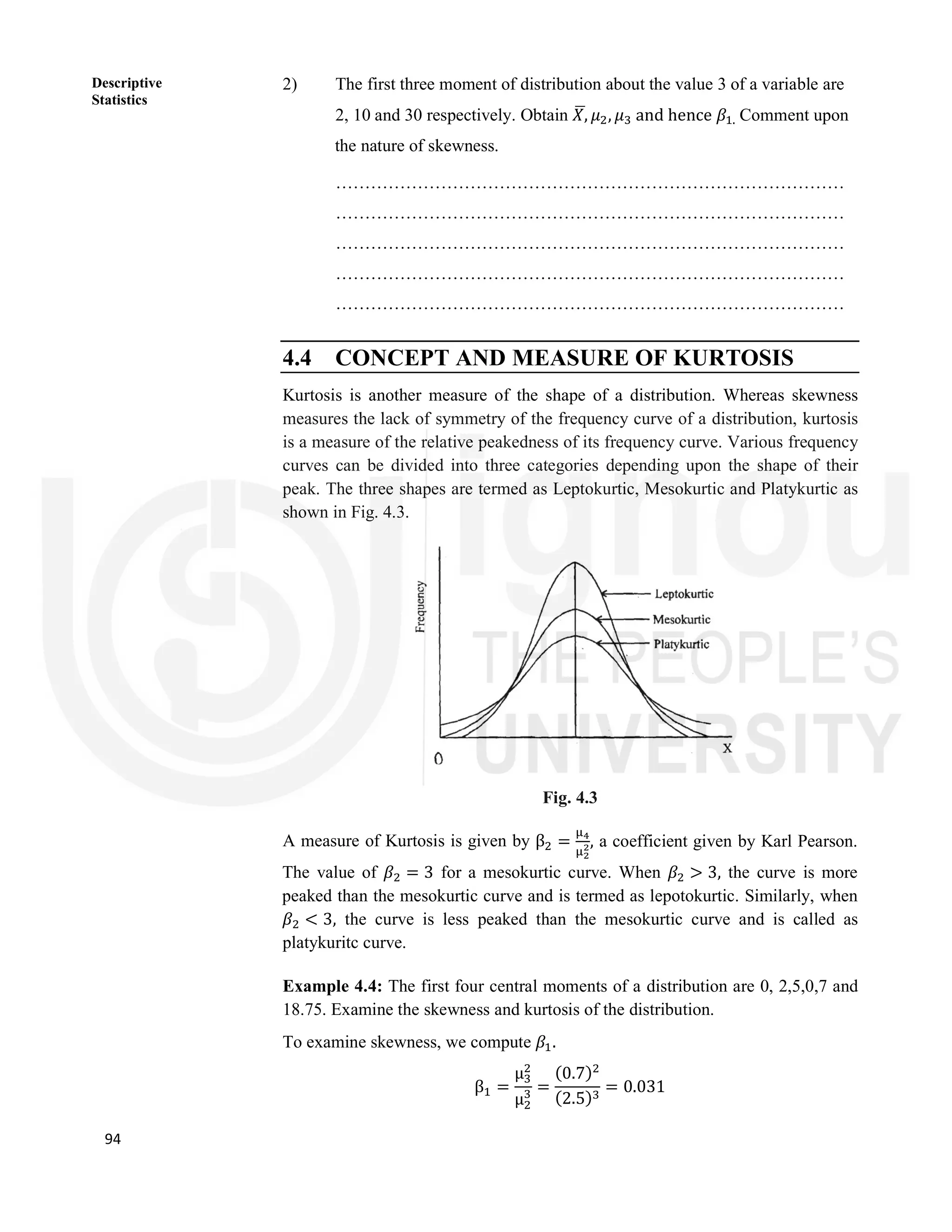
is a measure of the relative peakedness of its frequency curve. Various frequency
curves can be divided into three categories depending upon the shape of their
peak. The three shapes are termed as Leptokurtic, Mesokurtic and Platykurtic as
shown in Fig. 4.3.
Fig. 4.3
A measure of Kurtosis is given by β = , a coefficient given by Karl Pearson.
The value of 𝛽 = 3 for a mesokurtic curve. When 𝛽 > 3, the curve is more
peaked than the mesokurtic curve and is termed as lepotokurtic. Similarly, when
𝛽 < 3, the curve is less peaked than the mesokurtic curve and is called as
platykuritc curve.
Example 4.4: The first four central moments of a distribution are 0, 2,5,0,7 and
18.75. Examine the skewness and kurtosis of the distribution.
To examine skewness, we compute 𝛽 .
β =
μ
μ
=
(0.7)
(2.5)
= 0.031
95
Measures of Skewness
and Kurtosis
Since 𝜇 > 0 and 𝛽 is small, the distribution is moderately positively skewed.
Kurtosis is given by the coefficient
β =
μ
μ
=
18.75
(2.5)
= 3.0.
Hence the curve is mesokutic.
Check Your Progress 3
1) Compute the first four central moments from the following data. Also
find the two beta coefficients.
Value : 5 10 15 20 25 30 35
Frequency : 8 15 20 32 23 17 5
……………………………………………………………………………
……………………………………………………………………………
……………………………………………………………………………
……………………………………………………………………………
……………………………………………………………………………
2) The first four moments of a distribution are 1, 4, 10 and 46 respectively.
Compute the moment coefficients of skewness and kurtosis and comment
upon the nature of the distribution.
……………………………………………………………………………
……………………………………………………………………………
……………………………………………………………………………
……………………………………………………………………………
……………………………………………………………………………
4.5 LET US SUM UP
In this Unit you have learned about the measures of skeweness and kurtosis.
These two concepts are used to get an idea about the shape of the frequency
curve of a distribution. Skewness is a measure of the lack of symmetry whereas
kurtosis is a measure of the relative peakedness of the top of a frequency curve.
4.6 ANSWERS OR HINTS TO CHECK YOUR
PROGRSS EXERCISES
Check Your Progress 1
1) 0.237
2) – 0.12, – 0.243
3) 17.5, 54.38, 51.46
96
Descriptive
Statistics
Check Your Progress 2
1) 0,499.64, 2579.57, 589111.61, 0.053, skewness is positive.
2) 5,6, – 14, 0,907 since 𝜇 is negative the distribution is negatively skewed.
Check Your Progress 3
1) 0, 59.99, – 50.18, 8356.64, 0.012, (negatively skewed), 2.32 (platykurtic).
2) 0, 3. Thus the distribution is symmetrical and mesokurtic. Such a distribution
is also known as a Normal Distribution.

i-for-finance-and-banking-application-study-material.pdf

  • 1.
    UNIT 4 MEASURESOF SKEWNESS AND KURTOSIS Structure 4.0 Objectives 4.1 Introduction 4.2 Concept of Skewness 4.2.1 Karl Pearson's Measure of Skewness 4.2.2 Bowley's Measure of Skewness 4.2.3 Kelly's Measure of Skewness 4.3 Moments 4.4 Concept and Measure of Kurtosis 4.5 Let Us Sum Up 4.6 Answers or Hints to Check Your Progress Exercises 4.0 OBJECTIVES After going through this Unit, you will be able to:  distinguish between a symmetrical and a skewed distribution;  compute various coefficients to measure the extent o f skewness in a distribution;  distinguish between platykurtic, mesokurtic and leptokurtic distributions and  compute the coefficient of kurtosis. 4.1 INTRODUCTION In this unit you will learn various techniques to distinguish between various shapes of a frequency distribution. This is the final unit with regard to the summarization of univariate data. This unit will make you familiar with the concept of skewness and kurtosis. The need to study these concepts arises from the fact that the measures of central tendency and dispersion fail to describe a distribution completely. It is possible to have frequency distributions which differ widely in their nature and composition and yet may have same central tendency and dispersion. Thus, there is need to supplement the measures of central tendency and dispersion. Consequently, in this unit, we shall discuss two such measures, viz., measures of skewness and kurtosis.  Adapted from IGNOU study material of EEC 13: Elementary Statistical Methods and Survey Techniques, Units 4, 5 and 6 written by R S Bharadwaj with modifications by Kaustuva Barik
  • 2.
    85 Measures of Skewness andKurtosis 4.2 CONCEPT OF SKEWNESS The skewness of a distribution is defined as the lack of symmetry. In a symmetrical distribution, the Mean, Median and Mode are equal to each other and the ordinate at mean divides the distribution into two equal parts such that one part is the mirror image of the other (Fig. 6.1). If some observations, of very high (low) magnitude, are added to such a distribution, its right (left) tail gets elongated. Fig. 4.1 Fig. 4.2 These observations are also known as extreme observations. The presence of extreme observations on the right hand side of a distribution makes it positively skewed and the three averages, viz., mean, median and mode, will no longer be equal. For positively skewed distribution we find that: Mean > Median > Mode On the other hand, the presence of extreme observations to the left hand side of a distribution make it negatively skewed and the relationship between mean, median and mode is:
  • 3.
    86 Descriptive Statistics Mean < Median< Mode In Fig. 4.2 we depict the shapes of positively skewed and negatively skewed distributions. The direction and extent of skewness can be measured in various ways. We will discuss four measures of skewness in this unit. 4.2.1 Karl Pearson’s Measure of Skewness In Fig. 4.2 you noticed that the mean, median and mode are not equal in a skewed distribution. The Karl Pearson’s measure of skewness is based upon the divergence of mean from mode in a skewed distribution. Since Mean = Mode in a symmetrical distribution, (Mean – Mode) can be taken as an absolute measure of skewnes. The absolute measure of skewness for a distribution depends upon the unit of measurement. For example, if the mean = 2.45 metre and mode = 2.14 metre, then absolute measure of skewness will be 2.45 metre – 2.14 metre = 0.31 metre. For the same distribution, if we change the unit of measurement to centimeters, the absolute measure of skewness is 245 centimetre – 214 centimetre = 31 centimatre. In order to avoid such a problem Karl Pearson takes a relative measure of skewness. A relative measure, independent of the units of measurement, is defined as the Karl Pearson’s Coefficient of skewness Sk, given by 𝑆 = Mean − Mode s. d. The sign of 𝑆 gives the direction and its magnitude gives the extent of skewness. If 𝑆 > 0, the distribution is positively skewed, and if 𝑆 < 0 it is negatively skewed. Example 4.1: Compute the Karl Pearson’s coefficient of skewness from the following data: Height (in inches) Number of Persons 58 59 60 61 62 63 64 65 10 18 30 42 35 28 16 8 So far we have seen that 𝑆 is strategically dependent upon mode. If mode is not defined for a distribution we cannot find 𝑆 . The empirical relation between mean, median and mode states that, for a moderately symmetrical distribution, we have median and mode states that, for a moderately symmetrical distribution, we have Mean – Mode ≈3 (Mean – Median)
  • 4.
    87 Measures of Skewness andKurtosis Hence Karl Pearson’s coefficient of skewness is defined in terms of median as 𝑆 = 3(Mean − Mode) s. d. Table for the computation of mean and standard deviation (s.d.) Height (X) U = X – 61 No. of persons (f) fu fu2 58 59 60 61 62 63 64 65 -3 -2 -1 0 1 2 3 4 10 18 30 42 35 28 16 8 -30 -36 -30 0 35 56 48 32 90 72 30 0 35 112 144 128 Total 187 75 611 Mean = 61 + = 61.4 s. d. = 611 187 − 75 187 = 1.76 To find mode, we note that height is a continuous variable. It is assumed that the height has been measured under the approximation that a measurement on height that is, e.g., greater than 58 but less than 58.5 is taken as 58 inches while a measuring greater than or equal to 58.5 but less than 59 is taken as 59 inches. Thus the given data can be written as Height (in inches) Number of Persons 57.5 - 58.5 58.5 - 59.5 59.5 - 60.5 60.5 - 61.5 61.5 - 62.5 62.5 - 63.5 63.5 - 64.5 64.5 - 65.5 10 18 30 42 35 28 16 8 By inspection, the modal class in 60.5 – 61.5. Thus, we have 𝑙 = 60.5, ∆ = 42 − 30 = 12, ∆ = 42 − 35 = 7 and ℎ = 1 ∴ Mode = 60.5 + × 1 = 61.13 Hence, the Karl Pearson’s coefficient of skewness 𝑆 = . . . = 0.153. Thus the distribution is positively skewed.
  • 5.
    88 Descriptive Statistics 4.2.2 Bowley’s Measureof Skewness This measure is based on quartiles. For a symmetrical distribution, it is seen that 𝑄 and 𝑄 are equidistant from median. Thus (𝑄 − 𝑀 ) − (𝑀 − 𝑄 ) can be taken as an absolute measure of skewness. A relative measure of skewness, known as Bowley’s coefficient (𝑆 ), is given by 𝑆 = (𝑄 − 𝑀 ) − (𝑀 − 𝑄 ) (𝑄 − 𝑀 ) − (𝑀 − 𝑄 ) = 𝑄 − 2𝑀 + 𝑄 𝑄 − 𝑄 Let us calculate the Bowley’s coefficient for the following data on height of 187 persons: Height (in inches) Number of Persons(f) Cumulative Frequency 57.5 - 58.5 58.5 - 59.5 59.5 - 60.5 60.5 - 61.5 61.5 - 62.5 62.5 - 63.5 63.5 - 64.5 64.5 - 65.5 10 18 30 42 35 28 16 8 10 28 58 100 135 163 179 187 Computation of 𝑄 : Since = 46.75, the first quartile class is 59.5 – 60.5. Thus 𝑙 = 59.5, 𝐶 = 28, 𝑓 = 30 and ℎ = 1. ∴ 𝑄 = 59.59.5 + . × 1 = 60.125. Computation of 𝑀 (𝑄 ): Since = 93.5, the median class is 60.5 – 61.5. Thus 𝑙 = 60.5, 𝐶 = 58, 𝑓 = 42 and ℎ = 1. ∴ 𝑀 = 60.5 + × 1 = 61.345. Computation of 𝑄 : Since = 140.25, the third quartile class is 62.5 – 63.5. Thus 𝑙 = 62.5, 𝐶 = 135, 𝑓 = 28 and ℎ = 1. ∴ 𝑄 = 62.5 + . × 1 = 62.688. Hence, Bowley’s coefficient 𝑆 = . × . . . . = 0.048.
  • 6.
    89 Measures of Skewness andKurtosis 4.2.3 Kelly’s Measure of Skewness Bowley’s measure of skewness is based on the middle 50% of the observation because it leaves 25% of the observations on each extreme of the distribution. As an improvement over Bowley’s measure, Kelly has suggested a measure based on P10 and P90 so that only 10% of the observations on each extreme are ignored. Kelly’s coefficient of skewness, denoted by Sp, is given by 𝑆 = (𝑃 − 𝑃 ) − (𝑃 − 𝑃 ) (𝑃 − 𝑃 ) + (𝑃 − 𝑃 ) = 𝑃 − 2. 𝑃 + 𝑃 𝑃 − 𝑃 Note that 𝑃 = 𝑀 (median). The value of 𝑆 , for the data given in Table 6.1, can be computed as given below. Computation of 𝑃 : Since = × = 18.7, 10th percentile lies in the class 58.5 – 59.5. Thus 𝑙 = 58.5, 𝐶 = 10, 𝑓 = 18 and ℎ = 1. ∴ 𝑃 = 58.5 + × 1 = 58.983 Computation of 𝑃 : Since = × = 168.3, 90th percentile lies in the class 63.5 – 64.5. Thus 𝑙 = 63.5, 𝐶 = 163, 𝑓 = 16 and ℎ = 1. ∴ 𝑃 = 63.5 + . × 1 = 63.831 Hence, Kelly’s coefficient 𝑆 = . × . . . . = 0.026. It may be noted here that although the coefficient 𝑆 ,𝑆 and 𝑆 are not comparable, however, in the absence of skewness, each of them will be equal to zero. Check Your Progress 1 1) Compute the Karl Pearson’s coefficient of skewness from the following data: Daily Expenditure (Rs.): 0-20 20-40 40-60 60-80 80-100 No. of families: 13 25 27 19 16 …………………………………………………………………………… …………………………………………………………………………… …………………………………………………………………………… ……………………………………………………………………………
  • 7.
    90 Descriptive Statistics 2) The followingfigures relate to the size of capital of 285 companies: Compute the Bowley’s and Kelly’s coefficients of skewness and interpret the results. …………………………………………………………………………… …………………………………………………………………………… …………………………………………………………………………… …………………………………………………………………………… 3) The following measures were computed for a frequency distribution: Mean = 50, coefficient of Variation = 35% and Karl Pearson’s Coefficient of Skewness = ─ 0.25. Compute Standard Deviation, Mode and Median of the distribution. …………………………………………………………………………… …………………………………………………………………………… …………………………………………………………………………… …………………………………………………………………………… 4.3 MOMENTS The rth moment about mean of a distribution, denoted by μ , is given by μ = 1 𝑁 𝑓 (𝑋 − 𝑋) , where 𝑟 = 0, 1, 2, 3, 4, … … . . Thus, rth moment about mean is the mean of the rth power of deviations of observations from their arithmetic mean. In particular, if 𝑟 = 0, we have μ = 1 𝑁 𝑓(𝑋 − 𝑋) = 1, if 𝑟 = 1, we have μ = 1 𝑁 𝑓(𝑋 − 𝑋) = 0, if 𝑟 = 2, we have μ = 1 𝑁 𝑓 (𝑋 − 𝑋) = 𝜎 , if 𝑟 = 3, we have μ = 1 𝑁 𝑓 (𝑋 − 𝑋) and so on. These moments are also known as central moments. In addition to the above, we can define raw moments as moments about any arbitrary mean. Capital (in Rs. lacs.) 1-5 6-10 11-15 16-20 21-25 26-30 31-35 Total No. of companies 20 27 29 38 48 53 70 285
  • 8.
    91 Measures of Skewness andKurtosis Let A denote an arbitrary mean, then rth moment about A is defined as μ = 1 𝑁 𝑓 (𝑋 − 𝐴) , 𝑟 = 0, 1, 2, 3, … . . When A = 0, we get various moments about origin. Moment Measure of Skewness The moment measure of skewness is based on the property that, for a symmetrical distribution, all odd ordered central moments are equal to zero. We note that μ = 0, for every distribution, therefore, the lowest order moment that can provide an absolute measure of skewness is μ . Further, a coefficient of skewness, independent of the units of measurement, is given by α = = β = ± γ , where β and γ are defined as the first beta and first gamma coefficients respectively. Note that β is a measure of kurtosis as you will come to know in the next Section. Very often, the skewness is measured in terms of β = , where the sign of skewness is determined by the sign of μ . Example 4.2: Compute the Moment coefficient of skewness (β ) from the following data. Marks Obtained: 0-10 10-20 20-30 30-40 40-50 50-60 60-70 Frequency: 6 12 22 24 16 12 8 Table for the computations of mean, s.d. and 𝛍𝟑. Class Intervals Frequency (f) Mid- values(X) 𝑢 = 𝑋 − 35 10 𝑓𝑢 𝑓𝑢 𝑓𝑢 0-10 10-20 20-30 30-40 40-50 50-60 60-70 6 12 22 24 16 12 8 5 15 25 35 45 55 65 -3 -2 -1 0 1 2 3 -18 -24 -22 0 16 24 24 54 48 22 0 16 48 72 -162 -96 -22 0 16 96 216 Total 100 0 260 48 Since ∑ 𝑓𝑢 = 0, the mean of the distribution is 35. The second moment μ is equal to the variance (σ ) and its positive square root is equal to standard deviation (σ). μ = × 100 = 260, and s. d. (σ) = √260 = 16.12.
  • 9.
    92 Descriptive Statistics Also, μ =× 1000 = 480. Thus, β = ( ) ( ) = 0.01. Since the sign of 𝜇 is positive and β is small, the distribution is slightly positively skewed. If the mean of a distribution is not a convenient figure like 35, as in the above example, the computation of various central moments may become a cumbersome task. Alternatively, we can first compute raw moments and then convert them into central moments by using the equations obtained below. Conversion of Raw Moments into Central Moments We can write μ = 1 𝑁 𝑓 (𝑋 − 𝑋) = 1 𝑁 𝑓 [(𝑋 − 𝐴) − (𝑋 − 𝐴)] = 1 𝑁 𝑓 [(𝑋 − 𝐴) − μ ] (Sinceμ == 1 𝑁 𝑓 (𝑋 − 𝐴) = 𝑋 − 𝐴) Expanding the term within brackets by binomial theorem, we get = 1 𝑁 𝑓 𝑟∁ (𝑋 − 𝐴) μ − 𝑟∁ (𝑋 − 𝐴) μ + 𝑟∁ (𝑋 − 𝐴) μ − ⋯ = 1 𝑁 𝑓 (𝑋 − 𝐴) − 𝑟∁ 1 𝑁 𝑓 (𝑋 − 𝐴) μ + 𝑟∁ + 1 𝑁 𝑓 (𝑋 − 𝐴) μ − ⋯ From the above, we can write μ = μ − 𝑟∁ μ μ + 𝑟∁ μ μ − 𝑟∁ 𝑟∁ μ μ + ⋯ In particular, taking r = 2, 3, 4, etc., we get μ = μ − 2∁ μ + 2∁ μ μ = μ − μ (μ = 1) μ = μ − 3μ μ + 3μ − μ = μ − 3μ μ + 2μ μ = μ − 4μ μ + 6μ μ − 4μ + μ = μ − 4μ μ + 6μ μ − 3μ Example 4.3: Compute the first four moments about mean from the following data. Class Intervals: 0 – 10 10 – 20 20 – 30 30 – 40 Frequency (f) : 1 3 4 2 Table for computations of raw moments (Take A = 25).
  • 10.
    93 Measures of Skewness andKurtosis Class Intervals f Mid-Value 𝑢 = 𝑓𝑢 𝑓𝑢 𝑓𝑢 𝑓𝑢 0 – 10 1 5 – 2 – 2 4 -8 16 10 – 20 2 15 – 1 – 3 3 -3 3 20 – 30 3 25 0 0 0 0 0 30 – 40 4 35 1 2 2 2 2 Total 10 – 3 9 – 9 21 From the above table, we can write μ = −3 × 10 10 = −3, μ = 9 × 10 10 = 90, μ = −9 × 10 10 = −900 and μ = 21 × 10 10 = 2100 Moments about Mean By definition, μ = 0, μ = 90 − 9 = 81, μ = −900 − 3 × 90 × (−3) + 2 × (−3) = −900 + 810 − 54 = −144 and μ = 21000 − 4 × (−900) × (−3) + 6 × 90 × (−3) − 3 × (−3) = 21000 − 10800 + 4860 − 243 = 14817. Check Your Progress 2 1) Calculate the first four moments about mean for the following distribution. Also, calculate β and comment upon the nature of skewness. Class Intervals: 0 – 20 20 – 40 40 – 60 60 – 80 80 – 100 Frequency (f) : 8 28 35 17 12 …………………………………………………………………………… …………………………………………………………………………… …………………………………………………………………………… ……………………………………………………………………………
  • 11.
    94 Descriptive Statistics 2) The firstthree moment of distribution about the value 3 of a variable are 2, 10 and 30 respectively. Obtain 𝑋, 𝜇 , 𝜇 and hence 𝛽 . Comment upon the nature of skewness. …………………………………………………………………………… …………………………………………………………………………… …………………………………………………………………………… …………………………………………………………………………… …………………………………………………………………………… 4.4 CONCEPT AND MEASURE OF KURTOSIS Kurtosis is another measure of the shape of a distribution. Whereas skewness measures the lack of symmetry of the frequency curve of a distribution, kurtosis is a measure of the relative peakedness of its frequency curve. Various frequency curves can be divided into three categories depending upon the shape of their peak. The three shapes are termed as Leptokurtic, Mesokurtic and Platykurtic as shown in Fig. 4.3. Fig. 4.3 A measure of Kurtosis is given by β = , a coefficient given by Karl Pearson. The value of 𝛽 = 3 for a mesokurtic curve. When 𝛽 > 3, the curve is more peaked than the mesokurtic curve and is termed as lepotokurtic. Similarly, when 𝛽 < 3, the curve is less peaked than the mesokurtic curve and is called as platykuritc curve. Example 4.4: The first four central moments of a distribution are 0, 2,5,0,7 and 18.75. Examine the skewness and kurtosis of the distribution. To examine skewness, we compute 𝛽 . β = μ μ = (0.7) (2.5) = 0.031
  • 12.
    95 Measures of Skewness andKurtosis Since 𝜇 > 0 and 𝛽 is small, the distribution is moderately positively skewed. Kurtosis is given by the coefficient β = μ μ = 18.75 (2.5) = 3.0. Hence the curve is mesokutic. Check Your Progress 3 1) Compute the first four central moments from the following data. Also find the two beta coefficients. Value : 5 10 15 20 25 30 35 Frequency : 8 15 20 32 23 17 5 …………………………………………………………………………… …………………………………………………………………………… …………………………………………………………………………… …………………………………………………………………………… …………………………………………………………………………… 2) The first four moments of a distribution are 1, 4, 10 and 46 respectively. Compute the moment coefficients of skewness and kurtosis and comment upon the nature of the distribution. …………………………………………………………………………… …………………………………………………………………………… …………………………………………………………………………… …………………………………………………………………………… …………………………………………………………………………… 4.5 LET US SUM UP In this Unit you have learned about the measures of skeweness and kurtosis. These two concepts are used to get an idea about the shape of the frequency curve of a distribution. Skewness is a measure of the lack of symmetry whereas kurtosis is a measure of the relative peakedness of the top of a frequency curve. 4.6 ANSWERS OR HINTS TO CHECK YOUR PROGRSS EXERCISES Check Your Progress 1 1) 0.237 2) – 0.12, – 0.243 3) 17.5, 54.38, 51.46
  • 13.
    96 Descriptive Statistics Check Your Progress2 1) 0,499.64, 2579.57, 589111.61, 0.053, skewness is positive. 2) 5,6, – 14, 0,907 since 𝜇 is negative the distribution is negatively skewed. Check Your Progress 3 1) 0, 59.99, – 50.18, 8356.64, 0.012, (negatively skewed), 2.32 (platykurtic). 2) 0, 3. Thus the distribution is symmetrical and mesokurtic. Such a distribution is also known as a Normal Distribution.