The document outlines a project on performing exploratory data analysis (EDA) using Python, specifically on a retail dataset containing transaction data. Key findings include a high volume of transactions from the UK, significant variability in product pricing, and the presence of missing values and outliers that require further cleaning. Next steps suggested include investigating outliers and performing feature engineering for predictive modeling.

1. "How to Perform Exploratory Data
Analysis Using Python"
Presenter a
:
Abdullah Al Nafees
Affiliations:
a
Sylhet Engineering College (SEC), School of Applied Sciences & Technology, Shahjalal
University of Science and Technology, Tilagarh, Alurtol Road, Sylhet 3100, Bangladesh.
For Contact:
bdeshiresearchlabresource@gmail.com
Purpose: Coursera Project Completion Portfolio - Perform exploratory data analysis on retail data with Python

2. Introduction to EDA
What is Exploratory Data Analysis (EDA)?
• GTFS (General Transit Feed Specification) is
a standardized format used by public transit
agencies to share their schedule and route
information with developers.
• It enables developers to create applications
that provide users with accurate transit
information, such as trip planners and
schedule viewers.

3. Objectives of EDA
Discover patterns and trends.
Gain insights for hypothesis formation.
Prepare data for further modelling or analysis
Identify anomalies and outliers.

4. Dataset Description
 Dataset: Online Retail dataset.
 Number of Records Analysed:
5,000 (Sample).
 Key Columns:
• InvoiceNo: Transaction ID.
• StockCode: Product ID.
• Quantity: Number of units sold.
• UnitPrice: Price per unit.
• CustomerID: Customer identifier.
• Country: Customer's country.
 Dataset contains both numerical
and categorical data.
import pandas as pd
# Load dataset
df = pd.read_excel('Online Retail.xlsx')
# Basic information about the dataset
df.info()
# Display first few rows of the dataset
df.head()
Use Python's Pandas library to load and inspect the dataset.

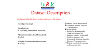
5. Missing Values
Handling Missing Values
• Description Column: 12 missing
values.CustomerID
• Column: Missing in a significant
number of rows (over 1,200
entries).
• Action Taken: Removed rows with
missing CustomerID for more
accurate analysis.
# Check for missing values in the dataset
df.isnull().sum()
# Drop rows with missing CustomerID
df_cleaned = df.dropna(subset=['CustomerID'])
# Confirm that missing values are handled
df_cleaned.isnull().sum()
• Identified missing values in Description and CustomerID columns.
• Rows with missing CustomerID were dropped for accurate analysis.

6. Descriptive Statistics
Descriptive Statistics of Numerical Data
 Quantity:
• Mean: 11.33 units per transaction.
• Max: 2,880 units (with some negative values
indicating returns).
• High variability with a standard deviation of 166.3.
 Unit Price:
• Mean: £3.18 per unit.
• Max: £295, showing a wide range in product pricing.
• Minimum: £0.03, likely discounted items or very
small products.
# Get summary statistics for numerical columns
df_cleaned[['Quantity', 'UnitPrice']].describe()
Use descriptive statistics to get insights into Quantity and Unit Price.

7. Country-wise Transaction Distribution
Top Countries by Transaction
Count
• The United Kingdom
accounts for the majority of
transactions (3,632).
• Norway, Germany, EIRE, and
France also contribute to
sales but on a much smaller
scale.
# Count transactions by country
country_sales = df_cleaned['Country'].value_counts()
# Show top 10 countries
country_sales.head(10)
Analyze the number of transactions per country.

8. Quantity vs Unit Price
Relationship between Quantity and Unit
Price
• Significant variance in Quantity and
UnitPrice across transactions.
• Some outliers with unusually high
quantities or prices, indicating
special orders or returns.
import matplotlib.pyplot as plt
# Scatter plot of Quantity vs UnitPrice
plt.scatter(df_cleaned['Quantity'], df_cleaned['UnitPrice'])
plt.xlabel('Quantity')
plt.ylabel('UnitPrice')
plt.title('Quantity vs Unit Price')
plt.show()
Use a scatter plot to visualize the relationship between Quantity
and Unit Price.

9. Outliers and Anomalies
Identifying Outliers and Anomalies
 Outliers were detected in both
Quantity and UnitPrice.
• Negative quantities indicate
product returns.
• Extremely high prices represent
expensive products.
 Further cleaning may be needed
to handle outliers.
import seaborn as sns
# Box plot for Quantity
sns.boxplot(x=df_cleaned['Quantity'])
plt.title('Box Plot of Quantity')
plt.show()
# Box plot for UnitPrice
sns.boxplot(x=df_cleaned['UnitPrice'])
plt.title('Box Plot of UnitPrice')
plt.show()
Identify outliers in Quantity and UnitPrice using a box plot.

10. Conclusion and Next Steps
Summary of Findings
 The majority of sales come
from the UK, with significant
variability in product prices and
quantities sold.
 Dataset contains missing values
and outliers that require further
cleaning.
 Next steps could include:
• Investigating the reasons for
outliers.
• Performing feature engineering
for predictive modelling.
# Further analysis and potential feature
engineering
df_cleaned['TotalPrice'] =
df_cleaned['Quantity'] *
df_cleaned['UnitPrice']
# Additional summary after feature
engineering
df_cleaned[['Quantity', 'UnitPrice',
'TotalPrice']].describe()
Present a clean summary with next steps.