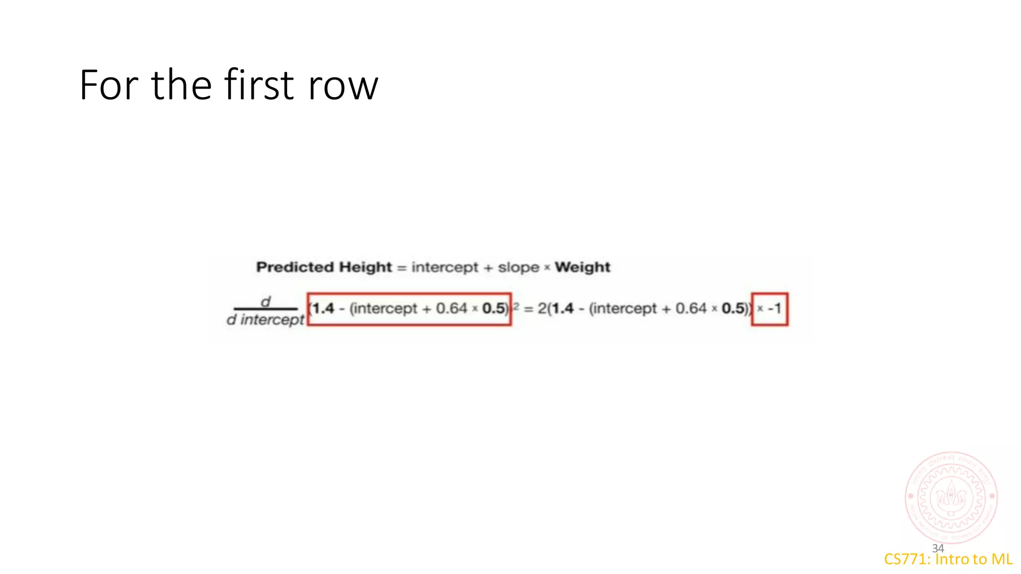
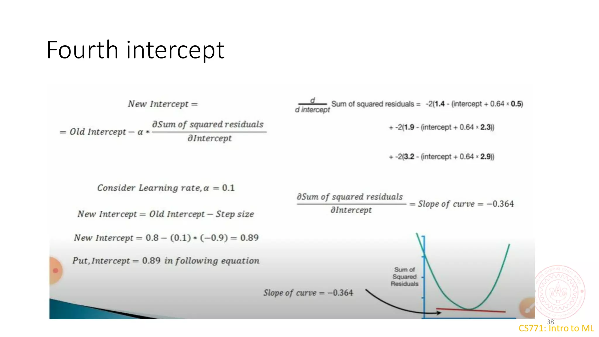
CS771: Intro to ML
Gradient descent algorithm
• Gradient descent algorithm is an optimization algorithm which is used to
minimise the function.
• The function which is set to be minimised is called as an objective
function.
• For machine learning, the objective function is also termed as the cost
function or loss function.
• Loss function is the measure of the squared difference between actual
values and predictions
CS771: Intro to ML
Gradient descent algorithm
2
• Gradient descent is an optimization algorithm used to
minimize some function by iteratively moving in the
direction of steepest descent .
• In machine learning, we use gradient descent to
update the parameters of our model. Parameters refer
to coefficients in Linear Regression
CS771: Intro to ML
CS771: Intro to ML
4
CS771: Intro to ML
5
Learning rate
• The size of these steps is called the learning rate.
• With a high learning rate we can cover more ground each step, but we
risk overshooting the lowest point since the slope of the hill is
constantly changing.
• A low learning rate is more precise, but calculating the gradient is
time-consuming, so it will take us a very long time to get to the
bottom.
CS771: Intro to ML
CS771: Intro to ML
7
CS771: Intro to ML
8
CS771: Intro to ML
9
CS771: Intro to ML
Local & Global Minima , Maxima
10
𝑓(𝑥)
Global
maxima
A local
maxima
A local
maxima
A local
minima
A local
minima A local
minima
Global
minima
𝑥
CS771: Intro to ML
the tangent is perfectly horizontal at the local minima and maxima.
CS771: Intro to ML
CS771: Intro to ML
Derivatives
13
 How the derivative itself changes tells us about the function’s optima
 The second derivative 𝑓’’(𝑥) can provide this information
𝑓’(𝑥)= 0 at 𝑥,
𝑓’(𝑥)>0 just
before 𝑥 𝑓’(𝑥)<0
just after 𝑥
𝑥 is a maxima
𝑓’(𝑥)= 0 at 𝑥
𝑓’(𝑥)< 0 just
before 𝑥 𝑓’(𝑥)>0
just after 𝑥
𝑥 is a minima
𝑓’(𝑥)= 0 at 𝑥
𝑓’(𝑥)= 0 just
before 𝑥 𝑓’(𝑥)= 0
just after 𝑥
𝑥 may be a saddle
𝑓’(𝑥)= 0 and 𝑓’’(𝑥) <
0
𝑥 is a maxima
𝑓’(𝑥)= 0 and 𝑓’’ 𝑥 > 0
𝑥 is a minima
𝑓’(𝑥)= 0 and 𝑓’’ 𝑥 = 0
𝑥 may be a saddle. May
need higher derivatives
CS771: Intro to ML
CS771: Intro to ML
Saddle Points
15
 Points where derivative is zero but are neither minima nor maxima
 Second or higher derivative may help identify if a stationary point is a
saddle
Saddle is a point of
inflection where the
derivative is also zero
A saddle
point
CS771: Intro to ML
Gradient Descent: An Illustration
16
𝒘∗
𝒘(0) 𝒘(1) 𝒘(2) 𝒘(0)
𝒘(1)
𝒘(2) 𝒘∗
𝒘(3) 𝒘(3)
Stuck at a
local minima
Negative gradient here (
𝛿𝐿
𝛿𝑤
<
0). Let’s move in the positive
direction
Positive gradient
here. Let’s move
in the negative
direction
Learning rate is very important
Good initialization
is very important
𝐿(𝒘)
𝒘
CS771: Intro to ML
CS771: Intro to ML
18
CS771: Intro to ML
19
CS771: Intro to ML
20
CS771: Intro to ML
21
CS771: Intro to ML
22
CS771: Intro to ML
23
CS771: Intro to ML
Optimal value of intercept ?
24
CS771: Intro to ML
Assume intercept=0
25
CS771: Intro to ML
For row =1
26
CS771: Intro to ML
For row =2 and row=3
27
CS771: Intro to ML
28
CS771: Intro to ML
29
CS771: Intro to ML
Different values of intercept
30
CS771: Intro to ML
Step 3
31
CS771: Intro to ML
Red line is the slope .. As the intercept
increases…
32
CS771: Intro to ML
33
CS771: Intro to ML
For the first row
34
CS771: Intro to ML
35
CS771: Intro to ML
36
CS771: Intro to ML
Third Intercept
37
CS771: Intro to ML
Fourth intercept
38
CS771: Intro to ML
39
CS771: Intro to ML
40

gradientDescentTNP (2).pdf

  • 1.
    CS771: Intro toML Gradient descent algorithm • Gradient descent algorithm is an optimization algorithm which is used to minimise the function. • The function which is set to be minimised is called as an objective function. • For machine learning, the objective function is also termed as the cost function or loss function. • Loss function is the measure of the squared difference between actual values and predictions
  • 2.
    CS771: Intro toML Gradient descent algorithm 2 • Gradient descent is an optimization algorithm used to minimize some function by iteratively moving in the direction of steepest descent . • In machine learning, we use gradient descent to update the parameters of our model. Parameters refer to coefficients in Linear Regression
  • 3.
  • 4.
  • 5.
    CS771: Intro toML 5 Learning rate • The size of these steps is called the learning rate. • With a high learning rate we can cover more ground each step, but we risk overshooting the lowest point since the slope of the hill is constantly changing. • A low learning rate is more precise, but calculating the gradient is time-consuming, so it will take us a very long time to get to the bottom.
  • 6.
  • 7.
  • 8.
  • 9.
  • 10.
    CS771: Intro toML Local & Global Minima , Maxima 10 𝑓(𝑥) Global maxima A local maxima A local maxima A local minima A local minima A local minima Global minima 𝑥
  • 11.
    CS771: Intro toML the tangent is perfectly horizontal at the local minima and maxima.
  • 12.
  • 13.
    CS771: Intro toML Derivatives 13  How the derivative itself changes tells us about the function’s optima  The second derivative 𝑓’’(𝑥) can provide this information 𝑓’(𝑥)= 0 at 𝑥, 𝑓’(𝑥)>0 just before 𝑥 𝑓’(𝑥)<0 just after 𝑥 𝑥 is a maxima 𝑓’(𝑥)= 0 at 𝑥 𝑓’(𝑥)< 0 just before 𝑥 𝑓’(𝑥)>0 just after 𝑥 𝑥 is a minima 𝑓’(𝑥)= 0 at 𝑥 𝑓’(𝑥)= 0 just before 𝑥 𝑓’(𝑥)= 0 just after 𝑥 𝑥 may be a saddle 𝑓’(𝑥)= 0 and 𝑓’’(𝑥) < 0 𝑥 is a maxima 𝑓’(𝑥)= 0 and 𝑓’’ 𝑥 > 0 𝑥 is a minima 𝑓’(𝑥)= 0 and 𝑓’’ 𝑥 = 0 𝑥 may be a saddle. May need higher derivatives
  • 14.
  • 15.
    CS771: Intro toML Saddle Points 15  Points where derivative is zero but are neither minima nor maxima  Second or higher derivative may help identify if a stationary point is a saddle Saddle is a point of inflection where the derivative is also zero A saddle point
  • 16.
    CS771: Intro toML Gradient Descent: An Illustration 16 𝒘∗ 𝒘(0) 𝒘(1) 𝒘(2) 𝒘(0) 𝒘(1) 𝒘(2) 𝒘∗ 𝒘(3) 𝒘(3) Stuck at a local minima Negative gradient here ( 𝛿𝐿 𝛿𝑤 < 0). Let’s move in the positive direction Positive gradient here. Let’s move in the negative direction Learning rate is very important Good initialization is very important 𝐿(𝒘) 𝒘
  • 17.
  • 18.
  • 19.
  • 20.
  • 21.
  • 22.
  • 23.
  • 24.
    CS771: Intro toML Optimal value of intercept ? 24
  • 25.
    CS771: Intro toML Assume intercept=0 25
  • 26.
    CS771: Intro toML For row =1 26
  • 27.
    CS771: Intro toML For row =2 and row=3 27
  • 28.
  • 29.
  • 30.
    CS771: Intro toML Different values of intercept 30
  • 31.
    CS771: Intro toML Step 3 31
  • 32.
    CS771: Intro toML Red line is the slope .. As the intercept increases… 32
  • 33.
  • 34.
    CS771: Intro toML For the first row 34
  • 35.
  • 36.
  • 37.
    CS771: Intro toML Third Intercept 37
  • 38.
    CS771: Intro toML Fourth intercept 38
  • 39.
  • 40.