Recommended
PDF
PDF
PDF
PDF
PDF
PDF
PPTX
DOCX
PDF
PDF
PPTX
PPTX
Tokyo nlp #8 label propagation
PDF
PDF
PDF
PPTX
Tokyo r24 r_graph_tutorial
PDF
PDF
PDF
KEY
KEY
KEY
KEY
KEY
KEY
KEY
KEY
KEY
PDF
More Related Content
PDF
PDF
PDF
PDF
PDF
PDF
PPTX
DOCX
Similar to ggplot2 に入門してみた
PDF
PDF
PPTX
PPTX
Tokyo nlp #8 label propagation
PDF
PDF
PDF
PPTX
Tokyo r24 r_graph_tutorial
PDF
PDF
PDF
More from Hidekazu Tanaka
KEY
KEY
KEY
KEY
KEY
KEY
KEY
KEY
KEY
PDF
ggplot2 に入門してみた 1. 2. 3. 4. 5. 本発表の内容
• 僕が ggplot2 というパッケージに入門した話
• ggplot2 の詳しい使い方は説明しません
• 詳しい使い方を知りたい人は、後で紹介する参考
文献を参照してください
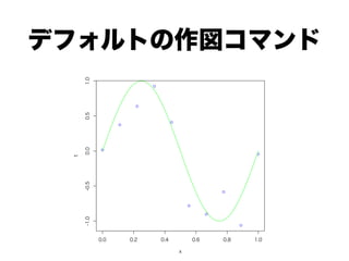
6. 7. 8. デフォルトの作図コマンド
1.0
0.5
0.0
t
-0.5
-1.0
0.0 0.2 0.4 0.6 0.8 1.0
x
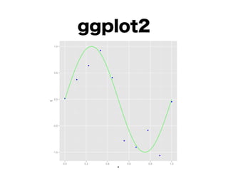
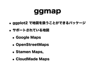
9. ggplot2
1.0
0.5
0.0
t
-0.5
-1.0
0.0 0.2 0.4 0.6 0.8 1.0
x
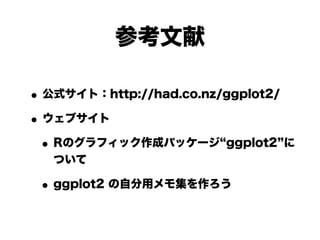
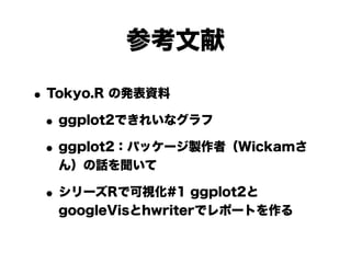
10. 11. 参考文献
• Tokyo.R の発表資料
• ggplot2できれいなグラフ
• ggplot2:パッケージ製作者(Wickamさ
ん)の話を聞いて
• シリーズRで可視化#1 ggplot2と
googleVisとhwriterでレポートを作る
12. 14. こいつは
藤村 こいつは
on
PRML
• パターン認識と機械学習
• 著者:C.M.ビショップ
• パターン認識や機械学習の各種のアルゴリズムや
背後の考え方について、ベイズ理論の観点から解
説した教科書
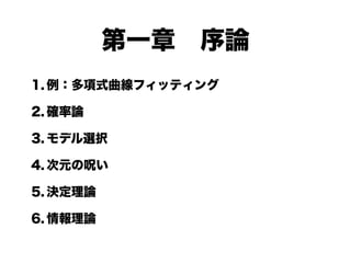
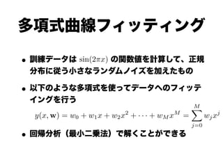
15. 16. 17. 多項式曲線フィッティング
• 訓練データは sin(2⇡x) の関数値を計算して、正規
分布に従う小さなランダムノイズを加えたもの
• 以下のような多項式を使ってデータへのフィッテ
イングを行う
M
X
2 M j
y(x, w) = w0 + w1 x + w2 x + · · · + wM x = wj x
j=0
• 回帰分析(最小二乗法)で解くことができる
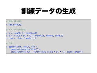
18. 訓練データの生成
# 乱数の種を設定
> sed.seed(3)
# テストデータの作成
> x <- seq(0, 1, length=10)
> t <- sin(2 * pi * x) + rnorm(10, mean=0, sd=0.3)
> test <- data.frame(x, t)
# 作図
> ggplot(test, aes(x, t)) +
geom_point(color="blue") +
stat_function(fun = function(x) sin(2 * pi * x), color="green")
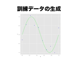
19. 訓練データの生成
1.0
0.5
t
0.0
-0.5
-1.0
0.0 0.2 0.4 0.6 0.8 1.0
x
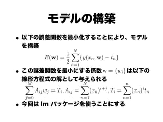
20. モデルの構築
• 以下の誤差関数を最小化することにより、モデル
を構築
XN
1
E(w) = {y(xn , w) tn }
2 n=1
• この誤差関数を最小にする係数 w = {wi} は以下の
線形方程式の解として与えられる
M
X N
X n
X
Aij wj = Ti , Aij = (xn )i+j , Ti = (xn )i tn
j=0 n=1 n=1
• 今回は lm パッケージを使うことにする
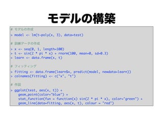
21. モデルの構築
# モデルの作成
> model <- lm(t~poly(x, 3), data=test)
# 訓練データの作成
> x <- seq(0, 1, length=100)
> t <- sin(2 * pi * x) + rnorm(100, mean=0, sd=0.3)
> learn <- data.frame(x, t)
# フィッティング
> fitting <- data.frame(learn$x, predict(model, newdata=learn))
> colnames(fitting) <- c("x", "t")
# 作図
> ggplot(test, aes(x, t)) +
geom_point(color="blue") +
stat_function(fun = function(x) sin(2 * pi * x), color="green") +
geom_line(data=fitting, aes(x, t), colour = "red")
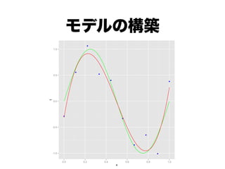
22. モデルの構築
1.0
0.5
t
0.0
-0.5
-1.0
0.0 0.2 0.4 0.6 0.8 1.0
x
23. モデルの構築
1.0 1.0
0.5 0.5
0.0 0.0
t
t
-0.5 -0.5
-1.0 -1.0
0.0 0.2 0.4 0.6 0.8 1.0 0.0 0.2 0.4 0.6 0.8 1.0
x x
1.0 1.0
0.5 0.5
0.0 0.0
t
t
-0.5 -0.5
-1.0 -1.0
0.0 0.2 0.4 0.6 0.8 1.0 0.0 0.2 0.4 0.6 0.8 1.0
x x
http://goo.gl/YEOeC
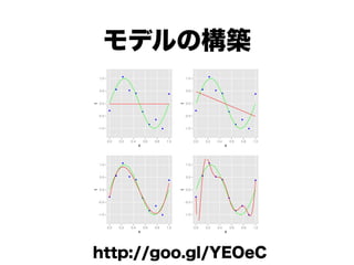
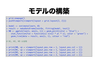
24. モデルの構築
> grid.newpage()
> pushViewport(viewport(layout = grid.layout(2, 2)))
> model <- estimate(learn, 0)
> result <- makeDataFrame(test$x, fitting(model, test))
> M0 <- ggplot(learn, aes(x, t)) + geom_point(color = "blue") +
stat_function(fun = function(x) sin(2 * pi * x), color = "green") +
geom_line(data = result, aes(x, t), colour = "red")
# M1, M3, M9 は省略
> print(M0, vp = viewport(layout.pos.row = 1, layout.pos.col = 1))
> print(M1, vp = viewport(layout.pos.row = 1, layout.pos.col = 2))
> print(M3, vp = viewport(layout.pos.row = 2, layout.pos.col = 1))
> print(M9, vp = viewport(layout.pos.row = 2, layout.pos.col = 2))
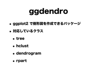
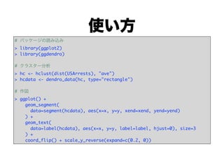
25. 26. 27. 使い方
# パッケージの読み込み
> library(ggplot2)
> library(ggdendro)
# クラスター分析
> hc <- hclust(dist(USArrests), "ave")
> hcdata <- dendro_data(hc, type="rectangle")
# 作図
> ggplot() +
geom_segment(
data=segment(hcdata), aes(x=x, y=y, xend=xend, yend=yend)
) +
geom_text(
data=label(hcdata), aes(x=x, y=y, label=label, hjust=0), size=3
) +
coord_flip() + scale_y_reverse(expand=c(0.2, 0))
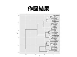
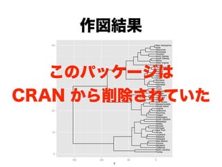
28. 作図結果
50 New Hampshire
Iowa
Wisconsin
Minnesota
Vermont
North Dakota
South Dakota
Maine
West Virginia
Hawaii
40 Pennsylvania
Connecticut
Kansas
Indiana
Utah
Ohio
Montana
Kentucky
Nebraska
Idaho
30 Texas
Colorado
Georgia
Tennessee
Arkansas
x
Missouri
New Jersey
Massachusetts
Rhode Island
Virginia
20 Oklahoma
Wyoming
Oregon
Washington
South Carolina
Mississippi
Alaska
Nevada
Michigan
New York
10 Illinois
Louisiana
Alabama
Delaware
New Mexico
Arizona
Maryland
California
North Carolina
Florida
0
150 100 50 0
y
29. 作図結果
50 New Hampshire
Iowa
Wisconsin
Minnesota
Vermont
North Dakota
South Dakota
Maine
West Virginia
Hawaii
このパッケージは
40 Pennsylvania
Connecticut
Kansas
Indiana
Utah
Ohio
Montana
Kentucky
Nebraska
Idaho
CRAN から削除されていた
30 Texas
Colorado
Georgia
Tennessee
Arkansas
x
Missouri
New Jersey
Massachusetts
Rhode Island
Virginia
20 Oklahoma
Wyoming
Oregon
Washington
South Carolina
Mississippi
Alaska
Nevada
Michigan
New York
10 Illinois
Louisiana
Alabama
Delaware
New Mexico
Arizona
Maryland
California
North Carolina
Florida
0
150 100 50 0
y
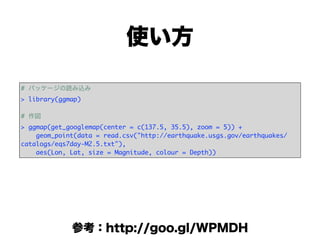
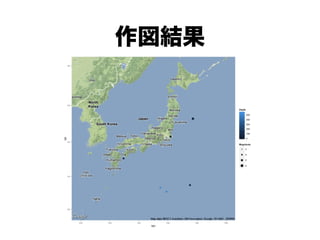
30. 31. 使い方
# パッケージの読み込み
> library(ggmap)
# 作図
> ggmap(get_googlemap(center = c(137.5, 35.5), zoom = 5)) +
geom_point(data = read.csv("http://earthquake.usgs.gov/earthquakes/
catalogs/eqs7day-M2.5.txt"),
aes(Lon, Lat, size = Magnitude, colour = Depth))
参考:http://goo.gl/WPMDH
32. 33.