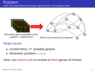
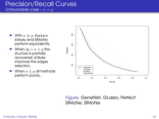
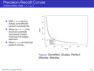
This document proposes a method for inferring sparse Gaussian graphical models with latent structure from biological data. It introduces a model that represents the concentration matrix as having a latent class structure, with vertices assigned to classes that determine their connectivity. An inference strategy alternates between estimating the latent class structure (E-step) and inferring the connectivity matrix (M-step). The method is evaluated on synthetic and breast cancer gene expression data.

1. Penalized Maximum Likelihood Inference for
Sparse Gaussian Graphical Models with
Latent Structure
Christophe Ambroise, Julien Chiquet and Catherine Matias
´
Laboratoire Statistique et Genome,
´ ´ ´
La genopole - Universite d’Evry
´
Statistique et sante publique, le 13 janvier 2009
Ambroise, Chiquet, Matias 1

2. Inferring Sparse Networks with Latent
Structure
Christophe Ambroise, Julien Chiquet and Catherine Matias
´
Laboratoire Statistique et Genome,
´ ´ ´
La genopole - Universite d’Evry
´
Statistique et sante publique, le 13 janvier 2009
Ambroise, Chiquet, Matias 1

3. Biological networks
Different kinds of biological interactions
dinI
SsB umD
Families of networks
lexA rpD rpH
protein-protein
interactions,
recA rpS
metabolic pathways,
recF
regulation network.
Regulation example : SOS Network E. Coli
Let us focus on regulatory networks . . . and look for influence
network
Ambroise, Chiquet, Matias 2

4. Biological networks
Different kinds of biological interactions
dinI
SsB umD
Families of networks
lexA rpD rpH
protein-protein
interactions,
recA rpS
metabolic pathways,
recF
regulation network.
Regulation example : SOS Network E. Coli
Let us focus on regulatory networks . . . and look for influence
network
Ambroise, Chiquet, Matias 2

5. Biological networks
Different kinds of biological interactions
dinI
SsB umD
Families of networks
lexA rpD rpH
protein-protein
interactions,
recA rpS
metabolic pathways,
recF
regulation network.
Regulation example : SOS Network E. Coli
Let us focus on regulatory networks . . . and look for influence
network
Ambroise, Chiquet, Matias 2

6. What questions?
What knowledge the structure
How to find the interactions? Network can provide?
Inference Structure
Degree
distri-
Un- bution
supervised
Given two nodes, do they
interact? Spectral
clustering
Supervised Community
analysis
Stat.
Given a new node, what are the
model
interaction with the known nodes?
Communities’ characteristics?
Ambroise, Chiquet, Matias 3

7. What questions?
What knowledge the structure
How to find the interactions? Network can provide?
Inference Structure
Degree
distri-
Un- bution
supervised
Given two nodes, do they
interact? Spectral
clustering
Supervised Community
analysis
Stat.
Given a new node, what are the
model
interaction with the known nodes?
Communities’ characteristics?
Ambroise, Chiquet, Matias 3

8. Problem
Infer the interactions between genes from microarray data
G5
G4 G6
G2
G3 G7
G0 G1
Microarray gene expression data, G9
p genes, n experiments Which ones interact/co-express? G8
Major Issues
2
combinatory: 2p possible graphs
dimension problem: n p
Here, we reduce p to a number of fixed genes of interest
Ambroise, Chiquet, Matias 4

9. Problem
Infer the interactions between genes from microarray data
G5
G4 G6
G2
Inference G3 G7
G0 G1
Microarray gene expression data, G9
p genes, n experiments Which ones interact/co-express? G8
Major Issues
2
combinatory: 2p possible graphs
dimension problem: n p
Here, we reduce p to a number of fixed genes of interest
Ambroise, Chiquet, Matias 4

10. Problem
Infer the interactions between genes from microarray data
G5
G4 G6
G2
Inference G3 G7
G0 G1
Microarray gene expression data, G9
p genes, n experiments Which ones interact/co-express? G8
Major Issues
2
combinatory: 2p possible graphs
dimension problem: n p
Here, we reduce p to a number of fixed genes of interest
Ambroise, Chiquet, Matias 4

11. Our ideas to tackle these issues
Introduce prior taking the topology of the network into
account for better edge inference
G5
G4 G6
G2
G3 G7
G0 G1
G9
G8
Relying on biological constraints
1. few genes effectively interact (sparsity),
2. networks are organized (latent structure).
Ambroise, Chiquet, Matias 5

12. Our ideas to tackle these issues
Introduce prior taking the topology of the network into
account for better edge inference
G5
G4 G6
G2
G3 G7
G0 G1
G9
G8
Relying on biological constraints
1. few genes effectively interact (sparsity),
2. networks are organized (latent structure).
Ambroise, Chiquet, Matias 5

13. Our ideas to tackle these issues
Introduce prior taking the topology of the network into
account for better edge inference
B3
B2 B4
A3
B1 B5
A1 A2
C2
C1
Relying on biological constraints
1. few genes effectively interact (sparsity),
2. networks are organized (latent structure).
Ambroise, Chiquet, Matias 5

14. Outline
Give the network a model
Gaussian graphical models
Providing the network with a latent structure
The complete likelihood
Inference strategy by alternate optimization
The E–step: estimation of the latent structure
The M–step: inferring the connectivity matrix
Numerical Experiments
Synthetic data
Breast cancer data
Ambroise, Chiquet, Matias 6

15. Outline
Give the network a model
Gaussian graphical models
Providing the network with a latent structure
The complete likelihood
Inference strategy by alternate optimization
The E–step: estimation of the latent structure
The M–step: inferring the connectivity matrix
Numerical Experiments
Synthetic data
Breast cancer data
Ambroise, Chiquet, Matias 6

16. Outline
Give the network a model
Gaussian graphical models
Providing the network with a latent structure
The complete likelihood
Inference strategy by alternate optimization
The E–step: estimation of the latent structure
The M–step: inferring the connectivity matrix
Numerical Experiments
Synthetic data
Breast cancer data
Ambroise, Chiquet, Matias 6

17. Outline
Give the network a model
Gaussian graphical models
Providing the network with a latent structure
The complete likelihood
Inference strategy by alternate optimization
The E–step: estimation of the latent structure
The M–step: inferring the connectivity matrix
Numerical Experiments
Synthetic data
Breast cancer data
Ambroise, Chiquet, Matias 7

18. GGMs
General settings
The Gaussian model
Let X ∈ Rp be a random vector such as X ∼ N (0p , Σ);
let (X 1 , . . . , X n ) be an i.i.d. size–n sample (e.g., microarray
experiments);
let X be a n × p matrix such as (X k ) is the kth row of X;
let K = (Kij )(i,j)∈P 2 := Σ−1 be the concentration matrix.
The graphical interpretation
Xi ⊥ Xj |XP{i,j} ⇔ Kij = 0 ⇔ edge (i, j) ∈ network,
⊥ /
since rij|P{i,j} = −Kij / Kii Kjj .
K describes the graph of conditional dependencies.
Ambroise, Chiquet, Matias 8

19. GGMs
General settings
The Gaussian model
Let X ∈ Rp be a random vector such as X ∼ N (0p , Σ);
let (X 1 , . . . , X n ) be an i.i.d. size–n sample (e.g., microarray
experiments);
let X be a n × p matrix such as (X k ) is the kth row of X;
let K = (Kij )(i,j)∈P 2 := Σ−1 be the concentration matrix.
The graphical interpretation
Xi ⊥ Xj |XP{i,j} ⇔ Kij = 0 ⇔ edge (i, j) ∈ network,
⊥ /
since rij|P{i,j} = −Kij / Kii Kjj .
K describes the graph of conditional dependencies.
Ambroise, Chiquet, Matias 8

20. GGMs and regression
Network inference as p independent regression problems
One may use p different linear regressions
Xi = (Xi ) α + ε, where αj = −Kij /Kii ,
¨
Meinshausen and Bulhman’s approach (06)
Solve p independent Lasso problems ( 1 –norm enforces
sparsity):
1 2
α = arg min Xi − Xi α 2 + ρ α 1 ,
α n
where Xi is the ith column of X, and Xi is the full matrix with ith
column removed.
Major drawback: need of a symmetrization step to obtain a
final estimate of K.
Ambroise, Chiquet, Matias 9

21. GGMs and regression
Network inference as p independent regression problems
One may use p different linear regressions
Xi = (Xi ) α + ε, where αj = −Kij /Kii ,
¨
Meinshausen and Bulhman’s approach (06)
Solve p independent Lasso problems ( 1 –norm enforces
sparsity):
1 2
α = arg min Xi − Xi α 2 + ρ α 1 ,
α n
where Xi is the ith column of X, and Xi is the full matrix with ith
column removed.
Major drawback: need of a symmetrization step to obtain a
final estimate of K.
Ambroise, Chiquet, Matias 9

22. GGMs and regression
Network inference as p independent regression problems
One may use p different linear regressions
Xi = (Xi ) α + ε, where αj = −Kij /Kii ,
¨
Meinshausen and Bulhman’s approach (06)
Solve p independent Lasso problems ( 1 –norm enforces
sparsity):
1 2
α = arg min Xi − Xi α 2 + ρ α 1 ,
α n
where Xi is the ith column of X, and Xi is the full matrix with ith
column removed.
Major drawback: need of a symmetrization step to obtain a
final estimate of K.
Ambroise, Chiquet, Matias 9

23. GGMs and Lasso
Solving p penalized regressions ⇔ maximize the penalized pseudo-likelihood
p
Consider the approximation P(X) = i=1 P(Xi |Xi ).
Proposition
The solution to
˜
K = arg max log L(X; K) + ρ K , (1)
1
K,Kij =Kji
with
p n
˜
L(X; K) = log P(Xik |Xi ; Ki ) ,
k
i=1 k=1
shares the same null-entries as the solution of the p
independent penalized regressions.
Those p terms are not independent, as K is not diagonal !
Still requires the post-symmetrization
Ambroise, Chiquet, Matias 10

24. GGMs and Lasso
Solving p penalized regressions ⇔ maximize the penalized pseudo-likelihood
p
Consider the approximation P(X) = i=1 P(Xi |Xi ).
Proposition
The solution to
˜
K = arg max log L(X; K) + ρ K , (1)
1
K,Kij =Kji
with
p n
˜
L(X; K) = log P(Xik |Xi ; Ki ) ,
k
i=1 k=1
shares the same null-entries as the solution of the p
independent penalized regressions.
Those p terms are not independent, as K is not diagonal !
Still requires the post-symmetrization
Ambroise, Chiquet, Matias 10

25. GGMs and penalized likelihood
The penalized likelihood of the Gaussian observations
Use a penalty term
n
(log det(K) − Tr(Sn K)) − ρ K 1 ,
2
where Sn is the empirical covariance matrix.
Banerjee et al. Model selection through sparse maximum
likelihood estimation for multivariate Gaussian, JMLR, 2008.
Ambroise, Chiquet, Matias 11

26. GGMs and penalized likelihood
The penalized likelihood of the Gaussian observations
Use a penalty term
n
(log det(K) − Tr(Sn K)) − ρ K 1 ,
2
where Sn is the empirical covariance matrix.
Natural generalization
Use different penalty parameters for different coefficients
n
(log det(K) − Tr(Sn K)) − ρZ (K) 1 ,
2
where ρZ (K) = (ρZi ,Zj (Kij ))i,j is a penalty function depending
on an unknown underlying structure Z.
Ambroise, Chiquet, Matias 11

27. Outline
Give the network a model
Gaussian graphical models
Providing the network with a latent structure
The complete likelihood
Inference strategy by alternate optimization
The E–step: estimation of the latent structure
The M–step: inferring the connectivity matrix
Numerical Experiments
Synthetic data
Breast cancer data
Ambroise, Chiquet, Matias 12

28. The concentration matrix structure
Modelling connection heterogeneity
Assumption: there exists a latent structure spreading the
vertices into a set Q = {1, . . . , q, . . . , Q} of classes of connectivity.
The classes of connectivity
Denote Z = {Zi = (Zi1 , . . . , ZiQ )}i where Ziq = 1{i∈q} are the
latent independent variables, with
α = {αq }, the prior proportions of groups,
(Zi ) ∼ M(1, α), a multinomial distribution.
A mixture of Laplace distributions
Assume Kij |Z independent. Then Kij | {Ziq Zj = 1} ∼ fq (·),
where
1 |x|
fq (x) = exp − , q, ∈ Q.
2λq λq
Ambroise, Chiquet, Matias 13

29. The concentration matrix structure
Modelling connection heterogeneity
Assumption: there exists a latent structure spreading the
vertices into a set Q = {1, . . . , q, . . . , Q} of classes of connectivity.
The classes of connectivity
Denote Z = {Zi = (Zi1 , . . . , ZiQ )}i where Ziq = 1{i∈q} are the
latent independent variables, with
α = {αq }, the prior proportions of groups,
(Zi ) ∼ M(1, α), a multinomial distribution.
A mixture of Laplace distributions
Assume Kij |Z independent. Then Kij | {Ziq Zj = 1} ∼ fq (·),
where
1 |x|
fq (x) = exp − , q, ∈ Q.
2λq λq
Ambroise, Chiquet, Matias 13

30. The concentration matrix structure
Modelling connection heterogeneity
Assumption: there exists a latent structure spreading the
vertices into a set Q = {1, . . . , q, . . . , Q} of classes of connectivity.
The classes of connectivity
Denote Z = {Zi = (Zi1 , . . . , ZiQ )}i where Ziq = 1{i∈q} are the
latent independent variables, with
α = {αq }, the prior proportions of groups,
(Zi ) ∼ M(1, α), a multinomial distribution.
A mixture of Laplace distributions
Assume Kij |Z independent. Then Kij | {Ziq Zj = 1} ∼ fq (·),
where
1 |x|
fq (x) = exp − , q, ∈ Q.
2λq λq
Ambroise, Chiquet, Matias 13

31. Some possible structures
Figure: From Affiliation to Bipartite
B3
B2 B4
Example
A3
Modular (affiliation) network
B1 B5 Two kinds of Laplace distributions
A1 A2 1. intra-cluster q = , fin (·; λin );
C2
2. inter-cluster q = , fout (·; λout ).
C1
Ambroise, Chiquet, Matias 14

32. Some possible structures
Figure: From Affiliation to Bipartite
B3
B2 B4
Example
A3
Modular (affiliation) network
B1 B5 Two kinds of Laplace distributions
A1 A2 1. intra-cluster q = , fin (·; λin );
C2
2. inter-cluster q = , fout (·; λout ).
C1
Ambroise, Chiquet, Matias 14

33. Outline
Give the network a model
Gaussian graphical models
Providing the network with a latent structure
The complete likelihood
Inference strategy by alternate optimization
The E–step: estimation of the latent structure
The M–step: inferring the connectivity matrix
Numerical Experiments
Synthetic data
Breast cancer data
Ambroise, Chiquet, Matias 15

34. Looking for a criteria. . .
We wish to infer non-null entries of K knowing the data. Then
our strategy is
ˆ
K = arg max P(K|X) = arg max log P(X, K).
K 0 K 0
Marginalization over Z
Because distribution of K is known conditional on the structure !
ˆ
K = arg max log Lc (X, K, Z),
K 0
Z∈Z
where Lc (X, K, Z) = P(X, K, Z) is complete-data likelihood.
An EM–like strategy is used hereafter to solve this problem.
Ambroise, Chiquet, Matias 16

35. Looking for a criteria. . .
We wish to infer non-null entries of K knowing the data. Then
our strategy is
ˆ
K = arg max P(K|X) = arg max log P(X, K).
K 0 K 0
Marginalization over Z
Because distribution of K is known conditional on the structure !
ˆ
K = arg max log Lc (X, K, Z),
K 0
Z∈Z
where Lc (X, K, Z) = P(X, K, Z) is complete-data likelihood.
An EM–like strategy is used hereafter to solve this problem.
Ambroise, Chiquet, Matias 16

36. Looking for a criteria. . .
We wish to infer non-null entries of K knowing the data. Then
our strategy is
ˆ
K = arg max P(K|X) = arg max log P(X, K).
K 0 K 0
Marginalization over Z
Because distribution of K is known conditional on the structure !
ˆ
K = arg max log Lc (X, K, Z),
K 0
Z∈Z
where Lc (X, K, Z) = P(X, K, Z) is complete-data likelihood.
An EM–like strategy is used hereafter to solve this problem.
Ambroise, Chiquet, Matias 16

37. The complete likelihood
Proposition
n
log Lc (X, K, Z) = (log det(K) − Tr(Sn K)) − ρZ (K) 1
2
− Ziq Zjl log(2λq ) + Ziq log αq + c,
i,j∈P,i=j i∈P,q∈Q
q, ∈Q
where Sn is the empirical covariance matrix and
ρZ (K) = ρZi Zj (Kij ) (i,j)∈P 2 is defined by
Kij
ρZi Zj (Kij ) = Ziq Zj .
λq
q, ∈Q
Ambroise, Chiquet, Matias 17

38. The complete likelihood
Proposition
n
log Lc (X, K, Z) = (log det(K) − Tr(Sn K)) − ρZ (K) 1
2
− Ziq Zjl log(2λq ) + Ziq log αq + c,
i,j∈P,i=j i∈P,q∈Q
q, ∈Q
where Sn is the empirical covariance matrix and
ρZ (K) = ρZi Zj (Kij ) (i,j)∈P 2 is defined by
Kij
ρZi Zj (Kij ) = Ziq Zj .
λq
q, ∈Q
Part concerning K: PML with a LASSO-type approach.
Ambroise, Chiquet, Matias 17

39. The complete likelihood
Proposition
n
log Lc (X, K, Z) = (log det(K) − Tr(Sn K)) − ρZ (K) 1
2
− Ziq Zjl log(2λq ) + Ziq log αq + c,
i,j∈P,i=j i∈P,q∈Q
q, ∈Q
where Sn is the empirical covariance matrix and
ρZ (K) = ρZi Zj (Kij ) (i,j)∈P 2 is defined by
Kij
ρZi Zj (Kij ) = Ziq Zj .
λq
q, ∈Q
Part concerning Z: estimation with a variational approach.
Ambroise, Chiquet, Matias 17

40. Outline
Give the network a model
Gaussian graphical models
Providing the network with a latent structure
The complete likelihood
Inference strategy by alternate optimization
The E–step: estimation of the latent structure
The M–step: inferring the connectivity matrix
Numerical Experiments
Synthetic data
Breast cancer data
Ambroise, Chiquet, Matias 18

41. An EM strategy
The conditional expectation to maximize
Q K|K(m) = E log Lc (X, K, Z)|X; K(m)
P Z|X, K(m) log Lc (X, K, Z)
Z∈Z
= P Z|K(m) log Lc (X, K, Z).
Z∈Z
Problem
No closed-form of Q K|K(m) because P(Z|K) cannot be
factorized.
We use variational approach to approximate P(Z|K).
Ambroise, Chiquet, Matias 19

42. An EM strategy
The conditional expectation to maximize
Q K|K(m) = E log Lc (X, K, Z)|X; K(m)
P Z|X, K(m) log Lc (X, K, Z)
Z∈Z
= P Z|K(m) log Lc (X, K, Z).
Z∈Z
Problem
No closed-form of Q K|K(m) because P(Z|K) cannot be
factorized.
We use variational approach to approximate P(Z|K).
Ambroise, Chiquet, Matias 19

43. Outline
Give the network a model
Gaussian graphical models
Providing the network with a latent structure
The complete likelihood
Inference strategy by alternate optimization
The E–step: estimation of the latent structure
The M–step: inferring the connectivity matrix
Numerical Experiments
Synthetic data
Breast cancer data
Ambroise, Chiquet, Matias 20

44. Variational estimation of the latent structure
Daudin et. al, 2008
Principle
Use an approximation R(Z) of P(Z|K) in the factorized form,
Rτ (Z) = i Rτ i (Zi ) where Rτ i is a multinomial distribution with
parameters τ i .
Maximize a lower bound of the log-likelihood
J (Rτ (Z)) = L(X, K) − DKL (Rτ (Z) P(Z|K)).
Using its tractable form, we have
J (Rτ (Z)) = Rτ (Z)Lc (X, K, Z) + H(Rτ (Z)).
Z
Ambroise, Chiquet, Matias 21

45. Variational estimation of the latent structure
Daudin et. al, 2008
Principle
Use an approximation R(Z) of P(Z|K) in the factorized form,
Rτ (Z) = i Rτ i (Zi ) where Rτ i is a multinomial distribution with
parameters τ i .
Maximize a lower bound of the log-likelihood
J (Rτ (Z)) = L(X, K) − DKL (Rτ (Z) P(Z|K)).
Using its tractable form, we have
J (Rτ (Z)) = Rτ (Z)Lc (X, K, Z) + H(Rτ (Z)).
Z
This term plays the role of E(Lc (X, K, Z)|X, K(m) )
Ambroise, Chiquet, Matias 21

46. Variational estimation of the latent structure
Daudin et. al, 2008
Principle
Use an approximation R(Z) of P(Z|K) in the factorized form,
Rτ (Z) = i Rτ i (Zi ) where Rτ i is a multinomial distribution with
parameters τ i .
Maximize a lower bound of the log-likelihood
J (Rτ (Z)) = L(X, K) − DKL (Rτ (Z) P(Z|K)).
Using its tractable form, we have
J (Rτ (Z)) = Rτ (Z)Lc (X, K, Z) + H(Rτ (Z)).
Z
This term plays the role of E(Lc (X, K, Z)|X, K(m) )
Maximizing J leads to a fix-point relationship for τ
Ambroise, Chiquet, Matias 21

47. Outline
Give the network a model
Gaussian graphical models
Providing the network with a latent structure
The complete likelihood
Inference strategy by alternate optimization
The E–step: estimation of the latent structure
The M–step: inferring the connectivity matrix
Numerical Experiments
Synthetic data
Breast cancer data
Ambroise, Chiquet, Matias 22

48. The M–step
Seen as a penalized likelihood problem
We aim at solving
K = arg max Qτ (K),
K 0
where
Penalized likelihood problem
n
Qτ (K) = (log det(K) − Tr(Sn K)) − ρτ (K) + Cst ,
2 1
Friedman, Hastie, Tibshirani. Sparse inverse covariance estimation
with the Lasso, Biostatistics, 2007.
Banerjee et al. Model selection through sparse maximum
likelihood estimation for multivariate Gaussian, JMLR, 2008.
We deal with a more complex penalty term here.
Ambroise, Chiquet, Matias 23

49. The M–step
Seen as a penalized likelihood problem
We aim at solving
K = arg max Qτ (K),
K 0
where
Penalized likelihood problem
n
Qτ (K) = (log det(K) − Tr(Sn K)) − ρτ (K) + Cst ,
2 1
Friedman, Hastie, Tibshirani. Sparse inverse covariance estimation
with the Lasso, Biostatistics, 2007.
Banerjee et al. Model selection through sparse maximum
likelihood estimation for multivariate Gaussian, JMLR, 2008.
We deal with a more complex penalty term here.
Ambroise, Chiquet, Matias 23

50. Let us work on the covariance matrix
Proposition
The maximization problem over K is equivalent to the following,
dealing with the covariance matrix Σ:
Σ= arg max log det(Σ),
(Σ−Sn )·/P ∞ ≤1
where · is the term-by-term division and
2 τiq τj
P = (pij )i,j∈P = .
n λq
q,
The proof use some optimization, primal/dual tricks
Ambroise, Chiquet, Matias 24

51. A Block-wise resolution
Denote
Σ11 σ 12 S11 s12 P11 p12
Σ= , Sn = , P= , (2)
σ 12 Σ22 s12 S22 p12 P22
where Σ11 is a (p − 1) × (p − 1) matrix, σ 12 is a p − 1 length
column vector and Σ22 is a scalar.
¨
Each column of Σ satisfies (by det of Schur complement)
−1
σ 12 = arg min y Σ11 y ,
{ (y−s12 )·/p12 ∞ ≤1}
Ambroise, Chiquet, Matias 25

52. A 1 –norm penalized writing
Proposition
Solving the block-wise problem is equivalent to solve the
following dual problem
2
1 1/2 −1/2
min Σ11 β − Σ11 s12 + p12 β ,
β 2 2
1
where is the term-by-term product. Vectors σ 12 and β are
linked by
σ 12 = Σ11 β/2.
A LASSO-like formulation with existing costless algorithms
Ambroise, Chiquet, Matias 26

53. The full EM algorithm
while Qτ (K(m) ) has not stabilized do
b b
//THE E-STEP: LATENT STRUCTURE INFERENCE
if m = 1 then
// First pass
Apply spectral clustering on the empirical covariance S to initialize τ
b
else
Compute τ with via fix-point algorithm, using K(m−1)
b b
end
//THE M-STEP: NETWORK INFERENCE
Construct the penalty matrix P according to τ
b
b (m) has not stabilized do
while Σ
for each column of Σb (m) do
Compute σ 12 by solving the LASSO–like problem with path-wise
b
coordinate optimization
end
end
b (m)
Compute K(m) by block-wise inversion of Σ
b
m←m+1
end
Ambroise, Chiquet, Matias 27

54. The full EM algorithm
while Qτ (K(m) ) has not stabilized do
b b
//THE E-STEP: LATENT STRUCTURE INFERENCE
if m = 1 then
// First pass
Apply spectral clustering on the empirical covariance S to initialize τ
b
else
Compute τ with via fix-point algorithm, using K(m−1)
b b
end
//THE M-STEP: NETWORK INFERENCE
Construct the penalty matrix P according to τ
b
b (m) has not stabilized do
while Σ
for each column of Σb (m) do
Compute σ 12 by solving the LASSO–like problem with path-wise
b
coordinate optimization
end
end
b (m)
Compute K(m) by block-wise inversion of Σ
b
m←m+1
end
Ambroise, Chiquet, Matias 27

55. The full EM algorithm
while Qτ (K(m) ) has not stabilized do
b b
//THE E-STEP: LATENT STRUCTURE INFERENCE
if m = 1 then
// First pass
Apply spectral clustering on the empirical covariance S to initialize τ
b
else
Compute τ with via fix-point algorithm, using K(m−1)
b b
end
//THE M-STEP: NETWORK INFERENCE
Construct the penalty matrix P according to τ
b
b (m) has not stabilized do
while Σ
for each column of Σb (m) do
Compute σ 12 by solving the LASSO–like problem with path-wise
b
coordinate optimization
end
end
b (m)
Compute K(m) by block-wise inversion of Σ
b
m←m+1
end
Ambroise, Chiquet, Matias 27

56. The full EM algorithm
while Qτ (K(m) ) has not stabilized do
b b
//THE E-STEP: LATENT STRUCTURE INFERENCE
if m = 1 then
// First pass
Apply spectral clustering on the empirical covariance S to initialize τ
b
else
Compute τ with via fix-point algorithm, using K(m−1)
b b
end
//THE M-STEP: NETWORK INFERENCE
Construct the penalty matrix P according to τ
b
b (m) has not stabilized do
while Σ
for each column of Σb (m) do
Compute σ 12 by solving the LASSO–like problem with path-wise
b
coordinate optimization
end
end
b (m)
Compute K(m) by block-wise inversion of Σ
b
m←m+1
end
Ambroise, Chiquet, Matias 27

57. Outline
Give the network a model
Gaussian graphical models
Providing the network with a latent structure
The complete likelihood
Inference strategy by alternate optimization
The E–step: estimation of the latent structure
The M–step: inferring the connectivity matrix
Numerical Experiments
Synthetic data
Breast cancer data
Ambroise, Chiquet, Matias 28

58. Outline
Give the network a model
Gaussian graphical models
Providing the network with a latent structure
The complete likelihood
Inference strategy by alternate optimization
The E–step: estimation of the latent structure
The M–step: inferring the connectivity matrix
Numerical Experiments
Synthetic data
Breast cancer data
Ambroise, Chiquet, Matias 29

59. Simulations settings
Five inference methods
1. InvCor
Edge estimation based on empirical correlation matrix inversion.
2. GeneNet (Strimmer et al.)
Edge estimation based on partial correlation with shrinkage.
3. GLasso (Friedman et al.)
Edge estimation uses a uniform penalty matrix.
4. “perfect” SIMoNe (best results our method can aspire to)
Edge estimation uses a penalty matrix constructed according to the theoretic
node classification.
5. SIMoNe (Statistical Inference for MOdular NEtworks)
Edge estimation uses a penalty matrix constructed according to the estimated
node classification, iteratively.
Ambroise, Chiquet, Matias 30

60. Test simulation setup
Simulated Graphs
Graphs simulated using an affiliation model (two sets of
parameters: intra-groups and inter-groups connections)
p = 200 nodes p(p − 1)/2 = 19900 possible interactions.
50 graphs (repetitions) were simulated per situation.
Gene expression data (i.e., Gaussian samples) was then
simulated using the sampled graph:
1. Favorable setting (n = 10p),
2. Middle case (n = 2p)
3. Unfavorable setting (n = p/2)
Unstructured graph
When no structure SIMoNe is comparable to GeneNet and
GLasso
Ambroise, Chiquet, Matias 31

61. Concentration matrix and structure
(a) (b) (c)
Figure: Simulation of the structured sparse concentration matrix.
Adjacency matrix without (a), with (b) columns reorganized
according the affiliation structure and corresponding graph (c).
Ambroise, Chiquet, Matias 32

62. Example of graph recovery
Favorable case
Figure: Theoretical graph and SIMoNe estimation
Ambroise, Chiquet, Matias 33

63. Example of graph recovery
Favorable case
Figure: Theoretical graph and SIMoNe estimation
Ambroise, Chiquet, Matias 33

64. Precision/Recall Curves
Definition
TP
Precision = = Proportion of true positives among all positives
TP + FP
TP
Recall = = Proportion of true positive among all edges
TP + FN
Ambroise, Chiquet, Matias 34

65. Precision/Recall Curves
Favorable setting – n = 10p
1.0
With n p, Perfect
0.8
SIMoNe and SIMoNe
perform equivalently
0.6
Precision
When 3p > n > p the
stucture is partially
0.4
recovered, SIMoNe
improves the edges
selection.
0.2
SIMoNe
GLasso
Perfect
When n ≤ p all methods GeneNet
Invcor
perform poorly. . .
0.0 0.2 0.4 0.6 0.8 1.0
Recall
Figure: GeneNet, GLasso, Perfect
SIMoNe, SIMoNe, InvCor
Ambroise, Chiquet, Matias 34

66. Precision/Recall Curves
Favorable setting – n = 6p
1.0
With n p, Perfect
0.8
SIMoNe and SIMoNe
perform equivalently
0.6
Precision
When 3p > n > p the
stucture is partially
0.4
recovered, SIMoNe
improves the edges
selection.
0.2
SIMoNe
GLasso
Perfect
When n ≤ p all methods GeneNet
Invcor
perform poorly. . .
0.0 0.2 0.4 0.6 0.8 1.0
Recall
Figure: GeneNet, GLasso, Perfect
SIMoNe, SIMoNe, InvCor
Ambroise, Chiquet, Matias 34

67. Precision/Recall Curves
Middle case – n = 3p
1.0
With n p, Perfect
0.8
SIMoNe and SIMoNe
perform equivalently
0.6
Precision
When 3p > n > p the
stucture is partially
0.4
recovered, SIMoNe
improves the edges
selection.
0.2
SIMoNe
GLasso
Perfect
When n ≤ p all methods GeneNet
Invcor
perform poorly. . .
0.0 0.2 0.4 0.6 0.8 1.0
Recall
Figure: GeneNet, GLasso, Perfect
SIMoNe, SIMoNe, InvCor
Ambroise, Chiquet, Matias 34

68. Precision/Recall Curves
Middle case – n = 2p
1.0
With n p, Perfect
0.8
SIMoNe and SIMoNe
perform equivalently
0.6
Precision
When 3p > n > p the
stucture is partially
0.4
recovered, SIMoNe
improves the edges
selection.
0.2
SIMoNe
GLasso
Perfect
When n ≤ p all methods GeneNet
Invcor
perform poorly. . .
0.0 0.2 0.4 0.6 0.8 1.0
Recall
Figure: GeneNet, GLasso, Perfect
SIMoNe, SIMoNe
Ambroise, Chiquet, Matias 34

69. Precision/Recall Curves
Unfavorable case – n = p
0.8
With n p, Perfect
SIMoNe and SIMoNe
perform equivalently
0.6
Precision
When 3p > n > p the
stucture is partially
0.4
recovered, SIMoNe
improves the edges
0.2
selection. SIMoNe
GLasso
When n ≤ p all methods Perfect
GeneNet
perform poorly. . .
0.0 0.2 0.4 0.6 0.8 1.0
Recall
Figure: GeneNet, GLasso, Perfect
SIMoNe, SIMoNe
Ambroise, Chiquet, Matias 34

70. Precision/Recall Curves
Unfavorable case – n = p/2
1.0
With n p, Perfect
0.8
SIMoNe and SIMoNe
perform equivalently
0.6
Precision
When 3p > n > p the
stucture is partially
0.4
recovered, SIMoNe
improves the edges
selection.
0.2
SIMoNe
GLasso
When n ≤ p all methods Perfect
GeneNet
perform poorly. . .
0.0 0.2 0.4 0.6 0.8 1.0
Recall
Figure: GeneNet, GLasso, Perfect
SIMoNe, SIMoNe
Ambroise, Chiquet, Matias 34

71. Outline
Give the network a model
Gaussian graphical models
Providing the network with a latent structure
The complete likelihood
Inference strategy by alternate optimization
The E–step: estimation of the latent structure
The M–step: inferring the connectivity matrix
Numerical Experiments
Synthetic data
Breast cancer data
Ambroise, Chiquet, Matias 35

72. First results on real a dataset
Prediction of the outcome of preoperative chemotherapy
Two types of patients
1. Patient response can be classified as either a pathologic
complete response (PCR)
2. or residual disease (Not PCR).
Gene expression data
133 patients (99 not PCR, 34 PCR)
26 identified genes (differential analysis)
Ambroise, Chiquet, Matias 36

73. First result on real a dataset
Prediction of the outcome of preoperative chemotherapy
MBTP_SI CA12
FGFRIOP
RAMPI
BB_S4
AMFR
ERBB4
IGFBP4
FLJI2650 BTG3
FLJ10916 GFRAI
METRN
GAMT
CTNND2 MAPT
SCUBE2
KIA1467 PDGFRA
E2F3 ZNF552
THRAP2 JMJD2B
RRM2
BECNI
MELK
Full Sample
Ambroise, Chiquet, Matias 37

74. First result on real a dataset
Prediction of the outcome of preoperative chemotherapy
CTNND2
CA12
FLJ10916
E2F3
MELK BB_S4
RRM2 KIA1467
ERBB4
JMJD2B
BECNI
GAMT
BTG3
SCUBE2
GFRAI ZNF552
MBTP_SI
THRAP2
METRN MAPT
AMFR
FLJI2650
FGFRIOP
IGFBP4
PDGFRA
RAMPI
Not PCR
Ambroise, Chiquet, Matias 37

75. First result on real a dataset
Prediction of the outcome of preoperative chemotherapy
MBTP_SI
RAMPI
ZNF552 JMJD2B
KIA1467
RRM2
THRAP2 MAPT
BB_S4
E2F3
METRN
BTG3 MELK
GAMT
BECNI
IGFBP4
CTNND2
SCUBE2
ERBB4 FLJ10916
GFRAI
FLJI2650
AMFR CA12
PDGFRA
FGFRIOP
PCR
Ambroise, Chiquet, Matias 37

76. Conclusions
To sum-up
We proposed an inference strategy based on a
penalization scheme given by an underlying unknown
structure.
The estimation strategy is based on a variational EM
algorithm, in which a L ASSO-like procedure is embedded.
Preprint on arxiv.
R package SIMoNe
Perspectives
Consider alternative prior more biologically relevant: hubs,
motifs.
Time segmentation when dealing with temporal data
Ambroise, Chiquet, Matias 38

77. Conclusions
To sum-up
We proposed an inference strategy based on a
penalization scheme given by an underlying unknown
structure.
The estimation strategy is based on a variational EM
algorithm, in which a L ASSO-like procedure is embedded.
Preprint on arxiv.
R package SIMoNe
Perspectives
Consider alternative prior more biologically relevant: hubs,
motifs.
Time segmentation when dealing with temporal data
Ambroise, Chiquet, Matias 38

78. Penalty choice (1)
Let Ci denote the connectivity component of i in the true
conditional dependency graph, and Ci the corresponding
component resulting from the estimate K.
Proposition
Fix some ε > 0 and choose the penalty parameters λ such that,
for all q, ∈ Q,
 
−1/2
2 1
2p2 Fn−2  max Sii Sjj − 2 (n − 2)1/2  ≤ ε,
nλq i=j λq
where 1 − Fn−2 is the c.d.f. of a Students’s t-distribution with
n − 2 degrees of freedom. Then
P(∃k, Ck Ck ) ≤ ε. (3)
Ambroise, Chiquet, Matias 39

79. Penalty choice (2)
It’s enough to choose λq such as
1/2
2 ε
λq (ε) ≥ n − 2 + t2
n−2
n 2p2
 −1/2
−1
ε
×  max Sii Sjj  tn−2 .
 
i=j 2p2
Ziq Zj =1
Ambroise, Chiquet, Matias 40

80. Penalty choice (3)
Practically,
Relax the λq in the E–step (variational inference), thus
making variational EM in the E-step.
Fix the λq in the M-step, adapting the above rule to the
context.
E.g., for an affiliation structure, we fix the ratio λin /λout = 1.2 and either let the
value 1/λin vary when considering precision/recall curves for synthetic data, or fix
this parameter relying on the above rule when dealing with real data
Ambroise, Chiquet, Matias 41