Downloaded 70 times
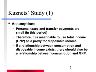
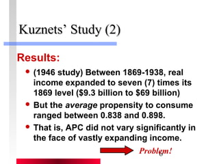
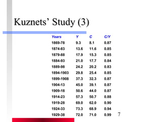
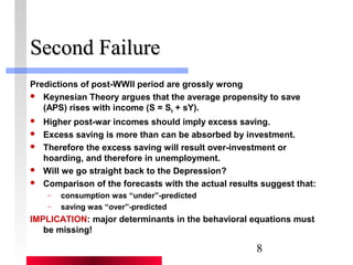
![10
LLCCHH ((22))
The consumption function implied by
this logic is:
C = 1 1 + ( -1) 1 +
[ e
] t
t t Y N Y A
T
with the aggregate estimable
consumption function look like this:
t
1
e
C bY b Y t t 2
b3A
1
1 = + +](https://image.slidesharecdn.com/froyen21-141030203849-conversion-gate02/85/Froyen21-10-320.jpg)
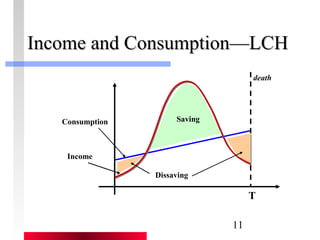
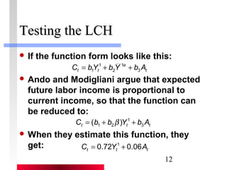
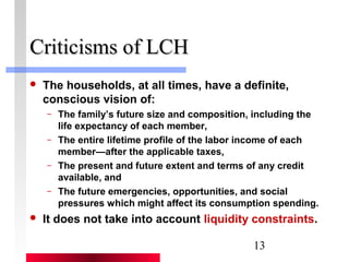
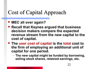

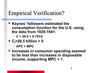
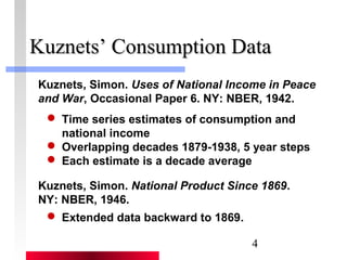
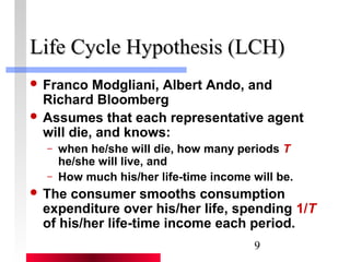
1) Keynes argued that consumption is determined by disposable income and other factors. Empirical studies from 1929-1941 estimated the consumption function as C = 26.5 + 0.75Yd, supporting Keynes' theory. 2) Kuznets' data from 1869-1938 showed average propensity to consume remained constant despite rising income, contradicting Keynesian predictions. 3) The life cycle and permanent income hypotheses were proposed as alternative explanations for consumption, arguing it depends on lifetime rather than current income. They better explained post-war consumption levels.


