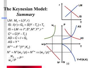
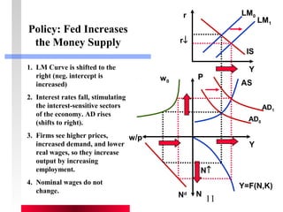
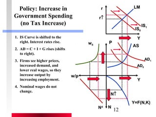
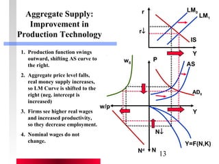
1. The document discusses the construction of the aggregate demand (AD) and aggregate supply (AS) curves from the IS-LM model. 2. It explains how the AD curve can be derived by observing how changes in the price level affect output and interest rates in the IS-LM model. 3. It then discusses sources of wage rigidity, including institutional factors like employment contracts, which allow the construction of the AS curve based on a fixed nominal wage level.

1. TThhee KKeeyynneessiiaann SSyysstteemm IIVV::
AAggggrreeggaattee SSuuppppllyy aanndd DDeemmaanndd
CChhaapptteerr 99
Professor Steve Cunningham
Intermediate Macroeconomics
ECON 219

2. 2
CCoonnssttrruuccttiinngg AADD
The AD curve can be constructed
from the IS-LM apparatus.
Recall that the price level is
established outside the IS-LM model.
We construct AD by observing the
how changes in the price level affect
the IS-LM model.

3. 3
LM(P0)
IS
LM(P2) r
LM(P1)
r2
r1
r0
Y2 Y1 Y0 Y
Y2 Y1 Y0
AD
P2
P1
P0
AADD ffrroomm IISS--LLMM
1. Price levels are
increased, with P0<P1<P2.
2. LM shifts to the left with
increasing P because real
money balances decline.
3. Interest rates rise.
4. Investment and durable
goods expenditures fall
as interest rates rise.
5. Plot prices levels against
the resulting output (Y)
levels.
6. This is aggregate
demand.
7. Thus AD is embedded in
the logic of IS-LM.

4. 4
CCoonnssttrruuccttiinngg AASS
To do this we go back to our
classical model and observe the
effects of having a fixed nominal
wage.
A less extreme view is to consider
nominal wages as being “sticky”—
meaning they adjust relatively
slowly.

5. SSoouurrcceess ooff WWaaggee RRiiggiiddiittyy ((11))
 General wage changes vs. relative wage
changes
 General wage changes
– If real wages (w/P) decline because of inflation
(P­), then everyone suffers the same. This is a
general real wage decline, and all workers are
equally affected.
– Thus workers are do not react as strongly to
this. Even if they did, there is little that they
could do about it.
5

6. SSoouurrcceess ooff WWaaggee RRiiggiiddiittyy ((22))
6
Relative wage change
– If an employer reduces the wages of an
individual worker, the worker’s relative
wage and buying power are affected.
– The worker may permanently have to
live decreased relative buying power.
– The worker may become disgruntled,
and labor supply may become reduced.

7. SSoouurrcceess ooff WWaaggee RRiiggiiddiittyy ((33))
7
Institutional factors:
– Workers often accept explicit or implicit
contracts for employment, accepting
that they will not be re-evaluated for
nominal wage changes for an extended
period.
– This leads to a contractual view of the
labor market.

8. 8
AS
Y
Nd Y=F(N,K)
w0
P
w/p
N
AS from
IS-LM

9. 9
AS
AD2
Y
Nd Y=F(N,K)
w0
P
w/p
N
AD0
AD1
N­
Y­
AD­
NOTES:
1. Employment and
output result from
AD increases.
2. That is, labor
demand is derived
demand. Firms
employ labor based
upon conditions in
the aggregate goods
and services market.
3. As prices rise, the
real wages fall,
making labor more
attractive.
4. As more workers are
employed, output
increases.
(w/p)¯

10. r LM
10
IS
Y
AS
Y
Y=F(N,K)
w0 P
Nd
w/p
N
AD
The Keynesian Model:
Summary
LM: ( , ) M0 = L Y r
0 0 0 IS : I(r ) +G = S(Y -T ) +T
IS = LM Þ I*,S*,M*,Y*,r *
* ( ) C = C Y -T0
AD = C + I +G0
AS =Y *
Nd = F-1 Y K
* ( *, ) 0
( / ) * ( / ) * N N w0 p N w0 p s = s = d Þ
*
w =
0 P
/ 0
w P

11. r LM0
11
IS
Y
AS
Y
LM1
Y=F(N,K)
w0 P
Nd
w/p
N
AD0
AD1
r¯
N­
Policy: Fed Increases
the Money Supply
1. LM Curve is shifted to the
right (neg. intercept is
increased)
2. Interest rates fall, stimulating
the interest-sensitive sectors
of the economy. AD rises
(shifts to right).
3. Firms see higher prices,
increased demand, and lower
real wages, so they increase
output by increasing
employment.
4. Nominal wages do not
change.

12. r LM
12
IS0
Y
AS
Y
Y=F(N,K)
w0 P
Nd
w/p
N
AD0
AD1
r­
N­
Policy: Increase in
Government Spending
(no Tax Increase)
1. IS Curve is shifted to the
right. Interest rates rise.
2. AD = C + I + G rises (shifts
to right).
3. Firms see higher prices,
increased demand, and
lower real wages, so they
increase output by
increasing employment.
4. Nominal wages do not
change.
IS1

13. r LM0
13
IS
Y
AS
Y
LM1
Y=F(N,K)
w0 P
Nd
w/p
N
AD0
r¯
N¯
Aggregate Supply:
Improvement in
Production Technology
1. Production function swings
outward, shifting AS curve to
the right.
2. Aggregate price level falls,
real money supply increases,
so LM Curve is shifted to the
right (neg. intercept is
increased)
3. Firms see higher real wages
and increased productivity,
so they decrease employment.
4. Nominal wages do not
change.

14. 14
LLiiqquuiiddiittyy TTrraapp
I
r
I
M
r
Md r*
Ms
M*
rˆ
S(Y)
S > I

15. 15
IInnvveessttmmeenntt TTrraapp
I
r
I
M
r
r*
Md
Ms
M*
S(Y)
r*
S > I

16. RReeaall BBaallaannccee EEffffeeccttss ((PPiiggoouu))
16
LM(P0)
IS
Y
r
r0
Y*
P1
IS+DG
LM(P1)
r1
AD1
Y
P
AD0
P0

17. RReeaall BBaallaannccee EEffffeeccttss ((PPiiggoouu))
17
IS
Y
r
r0=r1
Y0=Y1
P1
IS+DG
LM(P0)=LM(P1)
AD1
Y
P
AD0
P0
M
1
1
M 0
=
0
P
P