Download to read offline


![Synopsis
Au coeur des liens entre Théorie de la Démonstration et Théorie des Types se
trouve sans aucun doute la correspondance de Curry-Howard [How80]. Quels
avantages la Logique tire de ces liens n’est pas la question qui fait l’objet de la
présente thèse, dans laquelle on considère comme acquis le fait qu’il soit intel-
lectuelement désirable d’avoir en Logique:
• des objets mathématiques qui formalisent la notion de démonstration,
• des notions de calcul et de normalisation de ces objets,
• des théories équationnelles sur ces objets, c’est-à-dire des notions
d’équivalence, en relation avec les notions de calcul.
La correspondance de Curry-Howard fournit de tels concepts à la Logique en
connectant démonstrations et programmes d’une part, et proposition et types
d’autre part. Alors que son cadre originel était la déduction naturelle intuition-
iste [Gen35] (ou des systèmes à la Hilbert), les questions abordées par la présente
thèse se positionnent dans un cadre plus large, mais en mettant toujours l’accent
sur les notions d’équivalence et de normalisation. Plus précisément, elle contribue
à étendre le cadre des concepts fournis par la correspondance de Curry-Howard:
• à des formalismes en théorie de la démonstration (tels que le calcul des
séquents [Gen35]) qui sont appropriés à des considérations d’ordre logique
comme la recherche de démonstration (aussi appelée recherche de preuve),
• à des systèmes expressifs dépassant la logique propositionnelle tels que des
théories des types,
• aux raisonnements classiques plutôt qu’intuitionistes.
Les trois parties de cette thèse reflètent ces directions.
La première partie est intitulée Termes de Preuve pour la Logique Intu-
itioniste Implicationnelle; elle reste dans le cadre de la logique propositionnelle
intuitioniste (avec l’implication comme seul connecteur logique) mais elle étudie
les notions de la correspondance de Curry-Howard non seulement en déduction
naturelle mais aussi en calcul des séquents. Elle présente ainsi les termes (aussi
v](https://image.slidesharecdn.com/frenchenglish-150412084606-conversion-gate01/85/French-english-5-320.jpg)
![vi
appelés termes de preuve) avec lesquels sont représentés les démonstrations des
formalismes sus-mentionnés, ainsi que les avantages de l’utilisation, en déduction
naturelle, de règles issues du calcul des séquents, et enfin les notions de calcul
dans ce dernier formalisme et leurs liens avec les sémantiques d’appel par nom et
d’appel par valeur [Plo75].
La seconde partie est intitulée Théorie des Types en Calcul des Séquents;
elle reste dans le cadre de la logique intuitioniste et construit une théorie qui est
au calcul des séquents ce que les Systèmes de Types Purs [Bar92] sont à la déduc-
tion naturelle. Au delà des propriétés fondamentales de cette théorie sont aussi
étudiées des questions telles que la recherche de preuve et l’inférence de type.
La troisième partie est intitulée Vers la logique classique et est motivée
par l’objectif de construire en logique classique des théories similaires à celles
dévelopées dans la seconde partie en logique intuitioniste. En particulier, cette
partie dévelope un calcul des séquent correspondant au Système Fω [Gir72] mais
dont la couche des démonstrations est classique. Au delà d’une telle théorie des
types, la notion d’équivalence des démonstrations classiques devient cruciale et
la partie est conclue par une approche à ce problème.
La présente thèse aborde donc un grand nombre de questions, pour lesquelles
un cadre et une terminologie unifiés, les couvrant toutes, sont à la fois importants
et non-triviaux:
Chapitre 1
Ce chapitre présente les concepts et la terminologie utilisés dans le reste de la
thèse. Il présente tout d’abord les notions et notations concernant relations et
fonctions, comme les notions de (relation de) réduction, forte et faible simula-
tion, correspondance équationnelle, réflection, confluence, dérivation dans une
structure d’inférence. . .
Puis une partie importante est consacrée à la forte et la faible simulation ainsi
qu’aux techniques fondamentales pour prouver ces propriétés. Une considération
omniprésente dans cette partie est l’approche intuitioniste des résultats établis,
qui évite les raisonnements classiques commençant par “Supposons qu’il existe une
séquence de réduction infinie” et aboutissant à une contradiction. Par exemple la
technique de simulation est établie de manière intuitioniste, ainsi que les résultats
de forte normalisation des réductions lexicographiques et des réductions de multi-
ensembles.
Une autre partie importante de ce chapitre est consacrée aux calculs d’ordre
supérieur (HOC). En effet, les outils de la correspondance de Curry-Howard, dans
son cadre originel ou dans ceux abordés dans cette thèse, sont fondés sur des syn-
taxes de termes dont les constructeurs impliquent des liaisons de variables et
dont les relations de réduction sont définies par systèmes de réécriture [Ter03]
(que nous présentons avec les notions associées de redex, clôture contextuelle,
variable libre et muette, substitution,. . . ). De tels outils nécessitent un prudent](https://image.slidesharecdn.com/frenchenglish-150412084606-conversion-gate01/85/French-english-6-320.jpg)
![vii
traitement de l’α-equivalence (le fait que le choix d’une variable muette n’est
pas d’importance), en utilisant habituellement des conditions qui évitent la cap-
ture et la libération de variables. Dans la présente thèse nous écrirons rarement
ces conditions, précisément parce qu’elles peuvent être retrouvée mécaniquement
d’après le contexte où elle sont nécéssitées. Ce chapitre décrit comment.
Partie I
Chapitre 2
Ce chapitre présente la déduction naturelle, le calcul des séquents [Gen35] avec
(ou sans) sans règle de coupure, le λ-calcul [Chu41] avec sa notion de réduction ap-
pelée β-reduction, ainsi que la correspondance de Curry-Howard [How80]. Pour
cela, ce chapitre prolonge le chapitre 1 avec les concepts de sequent, système
logique, système de typage, terme de preuve, et la propriété de subject reduc-
tion, utilisés non seulement dans la partie I mais aussi dans le chapitre 10. Ce
chapitre est conclu par un calcul d’ordre supérieur pour représenter les démonstra-
tions du calcul des séquents intuitioniste G3ii, utilisé par exemple dans [DP99b].
Est remarqué le fait que le constructeur typé par une coupure est de la forme
d’une substitution explicite [ACCL91, BR95]. Les encodages de Gentzen et
Prawitz [Gen35, Pra65] entre la déduction naturelle et le calcul des séquents
sont exprimés ici comme des traductions de termes de preuves qui préservent le
typage.
Chapitre 3
Ce chapitre étudie le λ-calculus en appel par valeur (CBV) et part du calcul
λV [Plo75], qui restreint la β-reduction aux cas βV où l’argument d’une fonction est
déjà évalué comme valeur. On présente ensuite la sémantique CBV grâce à deux
variantes de traduction en Continuation Passing Style (CPS) dans des fragments
du λ-calcul : celle de Reynolds [Rey72, Rey98] et celle de Fischer [Fis72, Fis93].
On présente le calcul λC de Moggi qui étend λV [Mog88] d’une manière telle
que les traductions CPS deviennent des correspondances équationnelles [SF93,
SW97] : l’équivalence entre termes de λC générée par leurs réductions correspond
à l’équivalence entre leurs encodages générée par la β-reduction. Dans [SW97],
ceci est renforcé par le fait qu’un raffinement de la traduction de Reynolds forme
même une réflection. On prouve ici que c’est aussi le cas pour la traduction de
Fischer (si une modification mineure et naturelle de λC est faite), and l’on déduit
de cette réflection la confluence de λC (modifié). La modification et la réflection
aide aussi à établir un lien avec le calcul des séquents LJQ présenté au chapitre 6.](https://image.slidesharecdn.com/frenchenglish-150412084606-conversion-gate01/85/French-english-7-320.jpg)
![viii
Chapitre 4
Dans ce chapitre sont présentées deux techniques (qui peuvent être combinées)
pour prouver des propriétés de forte normalisation, en particulier des propriétés
de calculs proches du λ-calcul telles que la préservation de la forte normalisation
(PSN) [BBLRD96]. Ces deux techniques sont des raffinements de la technique de
simulation du chapitre 1.
Le point de départ de la première technique, appelée safeness and minimality
technique, est le fait que, pour prouver la forte normalisation, seules les réductions
de rédexes dont les sous-termes sont fortement normalisables ont besoin d’être
considérées (minimality). Ensuite, la notion de safeness fournit un critère utile
(selon que le rédex à réduire est fortement normalisable ou non) pour séparer les
réductions minimales en deux relations de réduction, dont la forte normalisation
peut être alors prouvée par composition lexicographique. L’exemple du calcul de
substitution explicites λx [BR95] illustre la technique, par des preuves courtes de
PSN, et de forte normalisation des termes simplement typés ou typés avec des
types intersection [CD78, LLD+
04].
La seconde technique fournit des outils pour prouver la forte normalisation
d’un calcul lié au λ-calcul, par simulation dans le λI-calcul de [Klo80] (fondé
sur les travaux antérieurs de [Chu41, Ned73]), si une simulation directe dans le
λ-calcul échoue. On démontre ainsi la propriété PSN pour λI. Cette seconde
technique est illustrée dans le chapitre 5.
Chapitre 5
Dans ce chapitre on présente un calcul d’ordre supérieur appelé λlxr dont la ver-
sion typée correspond, par la correspondance de Curry-Howard, à une version
multiplicative de la déduction naturelle intuitioniste. Celle-ci utilise des affaib-
lissements, des contractions and des coupures, habituels en calcul des séquents
(par exemple dans la version original de [Gen35]). Les constructeurs typés par les
règles sus-mentionnées peuvent être vus comme des constructeurs de ressources
gérant l’effacement et la duplication de substitutions explicites.
On décrit le comportement opérationnel de λlxr et ses propriétés fondamen-
tales, pour lesquels une notion d’équivalence sur les termes joue un rôle essentiel,
en particulier dans les réductions du calcul. Cette équivalence rapproche λlxr des
réseaux de preuve pour (le fragment intuitioniste de) la logique linéaire [Gir87]
(en fait [KL05, KL07] révèle une correspondance), mais elle est aussi nécessaire
pour que λlxr simule la β-réduction. Dans ce chapitre est établie une réflection du
λ-calculus dans λlxr, qui inclut la forte simulation de la β-reduction et entraîne la
confluence de λlxr. En utilisant la seconde technique dévelopée au chapitre 4, on
prouve aussi PSN et la forte normalisation des termes typés. λlxr est un calcul de
substitutions explicites qui a une notion de full composition et la propriété PSN.](https://image.slidesharecdn.com/frenchenglish-150412084606-conversion-gate01/85/French-english-8-320.jpg)
![ix
Chapitre 6
Dans ce chapitre est étudiée la notion de calcul dans le calcul des séquents in-
tuitioniste propositionnel —ici G3ii, fondée sur l’élimination des coupures. On
passe en revue trois types de systèmes d’élimination des coupures, tous forte-
ment normalisables sur les termes de preuve (typés), et l’on identifie une struc-
ture commune d’où sont définies les notions de réduction en appel par nom (CBN)
et en appel par valeur (CBV). On rappelle la t-restriction et la q-restriction dans
le calcul des séquents [DJS95, Her95] qui, dans le cas intuitioniste, mènent aux
fragments LJT et LJQ. Ceux-ci sont respectivement stables par réductions CBN
et CBV. On formalise par une réflection le lien entre LJT (et son calcul λ de
termes de preuve) et la déduction naturelle (et le λ-calcul). On prouve aussi PSN
pour λ, illustrant à nouveau la méthode de safeness and minimality dévelopée
au Chapitre 4. Le fragment LJQ est quant à lui connecté à la version du calcul
CBV λC [Mog88] présentée au chapitre 3.
Chapitre 7
Dans ce chapitre est appliquée la méthodologie des chapitre 2 et 6 (pour G3ii) au
calcul des séquents intuitioniste depth-bounded G4ii de [Hud89, Hud92, Dyc92].
On montre dans un premier temps comment l’on passe de LJQ à G4ii. Un cal-
cul de termes de preuve est ensuite présenté, utilisant des constructeurs corre-
spondant aux règles d’inférence admissibles dans le système (comme la règle de
coupure). Alors que les démonstrations traditionnelle d’admissibilité par induc-
tion suggèrent des transformations de démonstration faiblement normalisables,
on renforce ces approches en introduisant divers systèmes de réduction de terme
de preuve qui sont fortement normalisables. Les diverses variantes correspondent
à différentes optimisations, dont certaines sont orthogonales comme les sous-
systèmes CBN et CBV similaires à ceux de G3ii. Nous remarquons toutefois que
le sous-système CBV est plus naturel que celui CBN, ce qui est lié au fait que G4ii
est fondé sur LJQ.
Partie II
Chapitre 8
Fondés sur la déduction naturelle, les Systèmes de types purs (PTS) [Bar92] peu-
vent exprimer de nombreuses théories des types. Pour exprimer la recherche
de preuve dans de telles théories, on présente dans ce chapitre les Pure Type
Sequent Calculi (PTSC) en enrichissant LJT et le λ-calculus [Her95], presentés
au chapitre 6, car ils sont particulièrement adaptés à la recherche de preuve et
fortement liés à la déduction naturelle et au λ-calcul.](https://image.slidesharecdn.com/frenchenglish-150412084606-conversion-gate01/85/French-english-9-320.jpg)
![x
Les PTSC sont équippés d’une procédure de normalisation, adaptant celle de
λ et donc définie par des règles de réécriture locales en utilisant des substitutions
explicites. La propriété de subject reduction est démontrée et la réflection dans
λ du λ-calcul est adaptée en une réflection dans les PTSC des PTS. De plus,
le fait que la réflection préserve le typage montre qu’un PTSC est logiquement
équivalent au PTS correspondant. On démontre aussi que le premier est fortement
normalisable si et seulement si le deuxième l’est aussi.
Chapitre 9
Dans se chapitre sont étudiées des variantes des PTSC, essentiellement dévelop-
pées pour la recherche de preuve et l’inférence de type.
On montre comment les règles de conversion peuvent être incorporées aux
autres règles pour que les tactiques basiques de recherche de preuve soient sim-
plement l’application de bas en haut des règles d’inférence. Des variables d’ordre
supérieur (qui peuvent être vues comme des méta-variables) sont alors ajoutées
au formalisme ainsi que des contraintes d’unification, afin d’ajourner la réso-
lution de sous-buts dans la recherche de preuve et d’exprimer des algorithmes
d’énumération d’habitants de types similaire à ceux de [Dow93, Mun01].
On montre aussi comment les règles de conversion peuvent être incorporées
aux autres règles pour que l’inférence de type soit l’application de bas en haut des
règles d’inférence, d’un manière similaire au Constructive engine de la déduction
naturelle [Hue89, vBJMP94]. Pour cette section il est nécessaire d’introduire une
version des PTSC aux substitutions implicites, car l’inférence de type échoue avec
nos règles de typage pour les substitutions explicites.
Cette version avec substitutions implicites peut être aussi plus facilement
transformée en une version avec indices de de Bruijn, ce qui est fait dans la
dernière partie du chapitre, dans le style de [KR02].
Partie III
Chapitre 10
Dans ce chapitre on présente un système appelé FC
ω , une version du
Système Fω [Gir72] dans laquelle la couche des constructeurs de types est es-
sentiellement la même mais la prouvabilité des types est classique. Le calcul des
termes de preuve qui rend compte du raisonnement classique est une variante du
λ-calcul symétrique de [BB96].
On prouve que l’ensemble du calcul est fortement normalisable. Pour la couche
des constructeurs de types, on utilise la méthode de réductibilité de Tait et Girard,
combinée à des techniques d’orthogonalité. Pour la couche (classique) des termes
de preuve, on utilise la méthode de [BB96] fondée sur une notion symétrique de](https://image.slidesharecdn.com/frenchenglish-150412084606-conversion-gate01/85/French-english-10-320.jpg)
![candidats de réductibilité. Le système FC
ω , avec ses deux couches de différente
nature, est ainsi une opportunité de comparer les deux techniques et poser la
conjecture que la deuxième technique ne peut pas être subsumée par la première.
Nous concluons avec une preuve de cohérence de FC
ω , et un encodage du tra-
ditionel Système Fω dans FC
ω , même lorsque le premier utilise des axiomes sup-
plémentaires de la logique classique.
Chapitre 11
Tenter d’introduire des raisonnements classiques plus loin dans les théories des
types dévelopées en seconde partie (par exemple avec des types dépendants) se
heurte au problème de la définition d’une notion appropriée d’équivalence de dé-
monstrations classiques. Dans ce chapitre une approche originale est suggérée,
dans le cadre de la logique propositionnelle classique, et fondée sur le Calcul des
Structures [Gug, Gug02]. Les démonstrations sont des séquences de réécriture
sur les formules, et nous utilisons la notion de réduction parallèle [Tak89] pour
identifier différentes séquentialisations d’étapes de réécritures qui réduisent des
rédexes qui ne se chevauchent pas. Le cas des rédexes parallèles et celui des
rédexes imbriqués donnent lieu à deux notions d’équivalence sur les séquences de
réécriture (dans un système de réécriture linéaire qui formalise la logique clas-
sique). A partir de ces notions sont présentés deux formalismes qui autorisent
les réductions parallèles et ainsi fournissent un représentant canonique à deux
démonstrations équivalentes. Ce représentant peut être obtenu d’une démonstra-
tion quelconque par une relation de réduction particulière, qui est confluente and
qui termine (la confluence dans le cas des rédexes imbriqués n’est que conjec-
turée). Ces formalismes se révèlent être des calculs des séquents avec axiomes, et
leurs termes de preuves utilisent des combinateurs comme pour les systèmes à la
Hilbert. La procédure de normalisation qui produit les représentants canoniques
se trouve être une procédure de réduction des coupures.
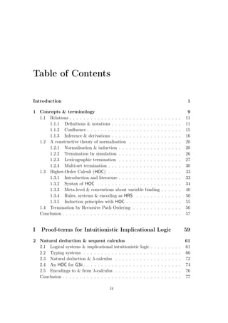
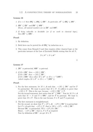
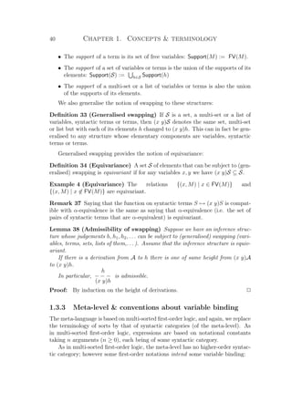
Dépendences entre chapitres
Pour faciliter la lecture de cette thèse et permettre certains chapitres d’être lus
indépendemment, le graphe de dépendence des chapitres est présenté dans la
Fig. 0, ainsi que les références bibliographiques dans lesquelles leur contenus, ou
certaines parties de leurs contenus, sont parus.
Les flèches pleines représentent une réelle dépendence (mais parfois seulement
parce qu’un chapitre utilise des définitions données dans un chapitre antérieur
mais familières au lecteur) ; les flèches en pointillés ne représentent qu’un lien
plus faible sans faire d’un chapitre le préalable d’un autre.](https://image.slidesharecdn.com/frenchenglish-150412084606-conversion-gate01/85/French-english-11-320.jpg)
![Définitions
générales
Logique
intuitioniste
Logique
classique
Chapitre 1
[Len05]
ÐÐ
Chapitre 2
xx
•–—™dfghjlm
o
ÔÔ
|| ~~|||||||||||||||||||
ÐÐ
××
Chapitre 3
44
‡ „ €
u
q
Chapitre 5
[KL05, KL07]
Chapitre 6
[DL06]
1
1
1
DDe d ™ — – • ” “ ‘ ‰
Chapitre 8
[LDM06]
ÑÑÔ
Ô
Ô
Ô
Ô
Ô
Ô
Ô
Ô
Ô
Ô
Chapitre 4
[Len05]
yy1
1
1
VVq
q
q
q
q
Chapitre 7
[DKL06]
Chapitre 9
Chapitre 10
[LM06]
xxq
q
q
q
q
Chapitre 11
[BL05]
Logique propositionnelle Théorie des types
Déduction
naturelle
Calcul des séquents
Fig. 0: Graphe de dépendence](https://image.slidesharecdn.com/frenchenglish-150412084606-conversion-gate01/85/French-english-12-320.jpg)

![Acknowledgements
It goes without saying that my greatest debt of gratitude is owed to my advisers
Delia Kesner and Roy Dyckhoff for all the time and energy that they have invested
in my thesis. Not only was I lucky to grow up in a biparental academic family,
but both of them provided the support and patience that a Ph.D. student could
hope for from a single adviser; the joint supervision was thus all the more fruitful,
eventually leading to [KL05, KL07, DL06, DKL06] and this dissertation.
Whilst they had a central role in making this cotutelle rewarding, it would not
have been possible without the initial efforts of Jacques Chevalier and the French
Embassy in London, whose plans met my Auld Alliance project at the right time.
With them I wish to thank Frank Riddell in St Andrews and other people from
each university whom I have not met, for pushing the cotutelle agreement through
many bureaucratic obstacles.
I am very grateful to Gilles Dowek and Luke Ong for agreeing to referee my
thesis, particularly in light of the work and time requisite in reading the 349
pages of this unexpectedly lengthy dissertation. I also wish to thank Pierre-
Louis Curien, Henk Barendregt, and Dale Miller for having accepted to sit on my
examination panel, and thus honoured me with their interest and time.
I thank James McKinna for the above reasons, and also for his role during
my time in St Andrews. Owing to his pioneering some of the ideas that Part II
investigates, his unique insight consolidated the progress I made. Part II thus
benefitted from numerous discussions with him, to the extent that his role therein
was that of an additional adviser, eventually leading to [LDM06]. I was met with
equal friendliness working with my other co-authors, such as Alexandre Miquel
and Kai Brünnler with whom joint work [LM06, BL05] was the origin of Part
III. They share a genuine and open-minded scientific curiosity that supported
my work. Alexandre’s grasp of Type Theory, pedagogical skills, patience, and
frequent after-dark presence at PPS made him a point of reference in the field to
which I regularly turn to. I appreciate in Kai his analytical mind and method-
ological approach to research, always having astute questions and concerns; a
memorable experience of skihock during a delightful wintery week-end in Bern
reminds me that his energy and enthusiasm to explore new and exotic ideas go
beyond academia.](https://image.slidesharecdn.com/frenchenglish-150412084606-conversion-gate01/85/French-english-16-320.jpg)


![Introduction
At the heart of the connections between Proof Theory and Type Theory undoubt-
edly lies the Curry-Howard correspondence [How80]. What Logic gains from these
connections is not the issue that we take as the purpose of this dissertation, in
which we rather take for granted the fact that are intellectually appealing such
concepts in Logic as:
• mathematical objects that can formalise the notion of proof,
• computational features of these objects with notions of normalisation,
• equational theories about these objects, that is to say, notions of equiva-
lence, that are related to their computational features.
The Curry-Howard correspondence provides such concepts to Logic by relating
proofs to programs and propositions to types, so that insight into one aspect
helps the understanding of the other. While its original framework was intuition-
istic propositional natural deduction [Gen35] (or Hilbert-style systems), this dis-
sertation investigates some issues pertaining to a more general framework, with
a particular emphasis on the notions of equivalence and normalisation. More
precisely, it contributes to broaden the scope of the concepts provided by the
Curry-Howard correspondence in three directions:
• proof-theoretic formalisms (such as sequent calculus [Gen35]) that are ap-
pealing for logical purposes such as proof-search,
• powerful systems beyond propositional logic such as type theories,
• classical reasoning rather than intuitionistic reasoning.
The three parts of this dissertation reflect these directions.
Part I is entitled Proof-terms for Intuitionistic Implicational Logic; it
remains within the framework of propositional intuitionistic logic (with impli-
cation as the only connective) but investigates the notions given by the Curry-
Howard correspondence in natural deduction as well as in sequent calculus. It
addresses such topics as the terms (a.k.a. proof-terms) with which the proofs of
these formalisms are represented, the benefits of using in natural deduction some
1](https://image.slidesharecdn.com/frenchenglish-150412084606-conversion-gate01/85/French-english-25-320.jpg)
![2 Introduction
rules of sequent calculus, the notions of computation in sequent calculus and their
relation with call-by-name and call-by-value semantics [Plo75].
Part II is entitled Type Theory in Sequent Calculus; it remains in the
framework of intuitionistic logic and builds a theory that is to sequent calculus
what Pure Type Systems [Bar92] are to natural deduction. Beyond the basic
properties of the theory, further aspects are developed, such as proof-search and
type inference.
Part III is entitled Towards Classical Logic and is motivated by the purpose
of building theories in classical logic such as those of Part II in intuitionistic logic.
In particular it develops a sequent calculus corresponding to System Fω [Gir72]
but whose layer of proofs is classical. Beyond such a type theory, the notion of
equivalence of classical proofs becomes crucial and the part concludes with an
approach to this issue.
This dissertation thus addresses a wide range of topics, for which a unified
framework and terminology, covering all of them, are thus both important and
non-trivial:
Chapter 1
This chapter introduces the concepts and the terminology that are used through-
out the three parts of the dissertation. It first introduces all notions and no-
tations about relations and functions, including reduction relation, strong and
weak simulation, equational correspondence, reflection, confluence, derivation in
an inference structure. . .
Then a major section is devoted to the notions of (weak and strong) nor-
malisation and basic techniques to prove these properties. A particular concern
of this section is to develop these ideas in a constructive setting, avoiding the
usual reasonings starting with “Let us assume that there is an infinite reduction
sequence,. . . ”, used especially when the strong normalisation of a reduction rela-
tion is inferred, by simulation, from that of another one that we already know to
be strongly normalising. We thus prove results about the strong normalisation
of the lexicographic composition of relations and the multi-set reduction relation.
Another major section of this chapter is devoted to Higher-Order Calculi. In-
deed, the tools for the Curry-Howard correspondence, whether in its original set-
ting or in the various ones tackled here, are based on syntaxes of terms involving
variable binding, with reduction relations given by rewrite systems [Ter03] which
we present together with the notions, traditional in rewriting, of redex, contextual
closure, free variables, substitution,. . . Such tools require a careful treatment of
α-equivalence (the fact that the choice of a variable that is bound is irrelevant),
usually using conditions to avoid variable capture and liberation. In this disser-
tation we deliberately not write these conditions, precisely because they can be
recovered mechanically from the context in which they are needed. This chapter
explains how.](https://image.slidesharecdn.com/frenchenglish-150412084606-conversion-gate01/85/French-english-26-320.jpg)
![Introduction 3
Part I
Chapter 2
This chapter introduces natural deduction, sequent calculus [Gen35] with (or
without) its cut-rule, λ-calculus [Chu41] with its notion of reduction called β-
reduction, and the Curry-Howard correspondence [How80]. For that it extends
Chapter 1 with such general concepts as sequents, logical systems, typing systems,
proof-terms, and subject reduction property, which will not only be used through-
out Part I but also in Chapter 10. It concludes by presenting an higher-order
calculus to represent proofs of the intuitionistic sequent calculus G3ii, as used for
instance in [DP99b]. It notes the fact that the constructor typed by a cut has
the shape of an explicit substitution [ACCL91, BR95]. Gentzen’s and Prawitz’s
encodings [Gen35, Pra65] between natural deduction and sequent calculus are
expressed here as type-preserving translations of proof-terms.
Chapter 3
In this chapter we investigate the call-by-value (CBV) λ-calculus. We start from
the calculus λV [Plo75], which merely restricts β-reduction to the case βV where
arguments of functions are already evaluated as values. We then present the CBV
semantics given by Continuation Passing Style (CPS) translations (into fragments
of λ-calculus), in two variants: Reynolds’ [Rey72, Rey98] and Fischer’s [Fis72,
Fis93]. We present Moggi’s λC-calculus [Mog88] that extends λV in a way such
that the CPS-translations become equational correspondences [SF93, SW97]. In
other words, the equivalence on λC-terms generated by their reductions matches
the equivalence between their encodings given by β-reduction. In [SW97] the
result is stronger in that (a refinement of) the Reynolds translation even forms
a reflection. In this chapter we prove that it is also the case for the Fischer
translation (if we make a minor and natural modification to λC), and we infer
from our reflection the confluence of (this modified) λC. The modification and
the reflection also help establishing a connection with a sequent calculus called
LJQ and presented in Chapter 6.
Chapter 4
In this chapter we present two techniques, which can be combined, to prove strong
normalisation properties, especially properties of calculi related to λ-calculus such
as Preservation of Strong Normalisation (PSN) [BBLRD96]. They are both re-
finements of the simulation technique from Chapter 1.
The first technique, called the safeness and minimality technique, starts with
the fact that, in order to prove strong normalisation, only the reduction of re-
dexes whose sub-terms are strongly normalising need to be looked at (minimal-](https://image.slidesharecdn.com/frenchenglish-150412084606-conversion-gate01/85/French-english-27-320.jpg)
![4 Introduction
ity). Then safeness provides a useful criterion (reducing redexes that are strongly
normalising or that are not) in order to split the (minimal) reductions of a calcu-
lus into two reduction relations, which can then be proved strongly normalising
by a lexicographic composition. The example of the explicit substitution calcu-
lus λx [BR95] illustrates the technique, with short proofs of PSN, strong nor-
malisation of the simply-typed version and that of its version with intersection
types [CD78, LLD+
04].
The second technique provides tools to prove the strong normalisation of a
calculus related to λ-calculus by simulation in the λI-calculus of [Klo80] (based
on earlier work by [Chu41, Ned73]), when a direct simulation in λ-calculus fails.
Such a tool is the PSN property for λI. This technique is illustrated in Chapter 5.
Chapter 5
In this chapter, we present a higher-order calculus called λlxr whose typed version
corresponds, via the Curry-Howard correspondence, to a multiplicative version of
intuitionistic natural deduction. The latter uses weakenings, contractions and
cuts, which are common in sequent calculus, e.g. in its original version [Gen35].
The constructors typed by the above rules can be seen as resource constructors
handling erasure and duplication of explicit substitutions.
We describe the operational behaviour of λlxr and its fundamental proper-
ties, for which a notion of equivalence on terms plays an essential role, in par-
ticular in the reduction relation of the calculus. This equivalence brings λlxr
close to the proof nets for (the intuitionistic fragment of) linear logic [Gir87] (in
fact [KL05, KL07] reveals a sound and complete correspondence), but it is also
necessary in order for λlxr to simulate β-reduction. In this chapter we actually
establish a reflection of λ-calculus in λlxr, which includes the strong simulation of
β-reduction and entails confluence of λlxr. Using the second technique developed
in Chapter 4, we also prove PSN, and strong normalisation of typed terms. λlxr is
an HOC with explicit substitutions having full composition and preserving strong
normalisation.
Chapter 6
In this chapter we investigate the notions of computation in intuitionistic propo-
sitional sequent calculus —here G3ii, based on cut-elimination. We survey three
kinds of cut-elimination system, proved or conjectured to be strongly normalis-
ing on typed terms, and identify a common structure in them, from which we
generically define call-by-name (CBN) and call-by-value (CBV) reductions. We
recall the t- and q-restrictions in sequent calculus [DJS95, Her95] which, in the
intuitionistic case, lead to the fragments LJT and LJQ of G3ii. These are stable
under CBN and CBV reductions, respectively. By means of a reflection we relate](https://image.slidesharecdn.com/frenchenglish-150412084606-conversion-gate01/85/French-english-28-320.jpg)
![Introduction 5
LJT, and its higher-order calculus λ that provides its proof-terms, to natural de-
duction and λ-calculus. We also prove PSN of λ as another illustration of the
safeness and minimality technique from Chapter 4. We then relate LJQ and its
proof-terms to (the modified version of) the CBV calculus λC [Mog88] presented
in Chapter 3.
Chapter 7
In this chapter we apply the methodology of Chapter 2 and Chapter 6 (for G3ii) to
the depth-bounded intuitionistic sequent calculus G4ii of [Hud89, Hud92, Dyc92].
We first show how G4ii is obtained from LJQ. We then present a higher-order
calculus for it —decorating proofs with proof-terms, which uses constructors cor-
responding to admissible rules such as the cut-rule. While existing inductive
arguments for admissibility suggest weakly normalising proof transformations,
we strengthen these approaches by introducing various term-reduction systems,
all strongly normalising on typed terms, representing proof transformations. The
variations correspond to different optimisations, some of them being orthogonal
such as CBN and CBV sub-systems similar to those of G3ii. We note however
that the CBV sub-system seems more natural than the CBN one, which is related
to the fact that G4ii is based on LJQ.
Part II
Chapter 8
Based on natural deduction, Pure Type Systems (PTS) [Bar92] can express a
wide range of type theories. In order to express proof-search in such theories, we
introduce in this chapter the Pure Type Sequent Calculi (PTSC) by enriching LJT
and the λ-calculus [Her95], presented in Chapter 6, because they are adapted to
proof-search and strongly related to natural deduction and λ-calculus.
PTSC are equipped with a normalisation procedure, adapted from that of λ
and defined by local rewrite rules as in cut-elimination, using explicit substitu-
tions. We prove that they satisfy subject reduction and turn the reflection in λ of
λ-calculus into a reflection in PTSC of PTS. Moreover, the fact that the reflection
is type-preserving shows that a PTSC is logically equivalent to its corresponding
PTS. Then we prove that the former is strongly normalising if and only if the
latter is.
Chapter 9
In this chapter we investigate variants of PTSC, mostly designed for proof-search
and type inference.](https://image.slidesharecdn.com/frenchenglish-150412084606-conversion-gate01/85/French-english-29-320.jpg)
![6 Introduction
We show how the conversion rules can be incorporated into the other rules so
that basic proof-search tactics in type theory are merely the root-first application
of the inference rules. We then add to this formalism higher-order variables (that
can be seen as meta-variables) and unification constraints, in order to delay the
resolution of sub-goals in proof-search and express type inhabitant enumeration
algorithms such as those of [Dow93, Mun01].
We also show how the conversion rules can be incorporated into the other
rules so that type inference becomes the root-first application of the inference
rules, in a way similar to the Constructive engine in natural deduction [Hue89,
vBJMP94]. For this section we also need to introduce a version of PTSC with
implicit substitutions, since type inference fails on our typing rule for explicit
substitutions.
This version with implicit substitutions is also easier to turn into a version
with de Bruijn indices, which we do in the final part of the chapter, in the style
of [KR02].
Part III
Chapter 10
In this chapter we present a system called FC
ω , a version of System Fω [Gir72] in
which the layer of type constructors is essentially the same whereas provability of
types is classical. The proof-term calculus accounting for the classical reasoning
is a variant of Barbanera and Berardi’s symmetric λ-calculus [BB96].
We prove that the whole calculus is strongly normalising. For the layer of
type constructors, we use Tait and Girard’s reducibility method combined with
orthogonality techniques. For the (classical) layer of terms, we use Barbanera and
Berardi’s method based on a symmetric notion of reducibility candidates. System
FC
ω , with its two layers of different nature, is thus an opportunity to compare the
two above techniques and raise the conjecture that the latter cannot be captured
by the former.
We conclude with a proof of consistency for FC
ω , and an encoding from the
traditional System Fω into FC
ω , also when the former uses extra axioms to allow
classical reasonings.
Chapter 11
Trying to introduce classical reasonings further inside the type theories developed
in Part II, namely when these feature dependent types, runs into the problem of
defining a suitable notion of equivalence for classical proofs. In this chapter we
suggest an original approach, in the framework of classical propositional logic,
based on the Calculus of Structures [Gug, Gug02]. Proofs are rewrite sequences](https://image.slidesharecdn.com/frenchenglish-150412084606-conversion-gate01/85/French-english-30-320.jpg)
![Introduction 7
on formulae, and we use the notion of parallel reduction [Tak89] to collapse bu-
reaucratic sequentialisations of rewrite steps that reduce non-overlapping redexes.
The case of parallel redexes and that of nested redexes give rise to two notions
of equivalence on rewrite sequences (according to a linear rewrite system that
formalises classical logic). We thence introduce two formalisms that allow par-
allel rewrite steps, thus providing to equivalent proofs a single representative.
This representative can be obtained from any proof in the equivalence class by
a particular reduction relation, which is confluent and terminating (confluence
in the case of nested redexes is only conjectured). These formalisms turn out to
be sequent calculi with axioms and proof-terms for them use combinators as in
Hilbert-style systems. The normalisation process that produce canonical repre-
sentatives is then a cut-reduction process.
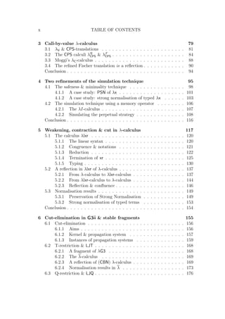
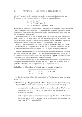
Dependencies between chapters
To facilitate the reading of this dissertation and allow particular chapters to be
read independently, we show in Fig. 1 the dependency graph of chapters, together
with the references where some or all of their contents already appeared.
Full arrows represent a real dependency (but sometimes only because a chap-
ter uses definitions, given in another chapter, of notions that are familiar to the
reader), while dashed arrows represent only a weak connection without making
one chapter a prerequisite for the other.](https://image.slidesharecdn.com/frenchenglish-150412084606-conversion-gate01/85/French-english-31-320.jpg)
![8 Introduction
General
definitions
Intuitionistic
logic
Classical
logic
Chapter 1
[Len05]
ÐÐ
Chapter 2
xx
“•–—™dfgijlm
o
ÔÔ
|| ~~}}}}}}}}}}}}}}}}}}}
ÑÑ
××
Chapter 3
33
‡ „ €
u
p
Chapter 5
[KL05, KL07]
Chapter 6
[DL06]
1
1
1
DDe d ™ ˜ – • ” ’ ‘ ‰
Chapter 8
[LDM06]
ÒÒÕ
Õ
Õ
Õ
Õ
Õ
Õ
Õ
Õ
Õ
Õ
Chapter 4
[Len05]
yy1
1
1
VVq
q
q
q
q
Chapter 7
[DKL06]
Chapter 9
Chapter 10
[LM06]
yyr
r
r
r
r
Chapter 11
[BL05]
Propositional logic Type theories
Natural
deduction
Sequent calculus
Figure 1: Dependency graph](https://image.slidesharecdn.com/frenchenglish-150412084606-conversion-gate01/85/French-english-32-320.jpg)
![10 Chapter 1. Concepts terminology
ment [Coq94] of Ramsey theory.
Most of the material in this section can be found in various textbooks
(e.g. [Ter03]), but perhaps not always with constructive proofs, and we intend to
make this dissertation self-contained.
A first version of this section, together with the major part of chapter 4,
appeared as the technical report [Len05].
Section 1.3 describes how the rest of the dissertation treats higher-order cal-
culi, i.e. calculi involving variable binding. Again, a good overview of formalisms
describing higher-order formalisms can be found in [Ter03].
Objects of the theory are α-equivalence classes of terms, and variable binding
requires us to take care of such problems as variable capture and variable libera-
tion, constantly juggling between α-equivalence classes and their representatives.
Reasonings about higher-order calculi are thus tricky: formalising them prop-
erly in first-order logic, where terms have no intrinsic notion of binding, might re-
quire a lot of side-conditions and lemmas (e.g. about renaming, name-indifference,
etc.).
Whether or not such a heavy formalisation is in fact helpful for the reader’s
understanding might be questioned. It could be argued that a human mind is
rather distracted from the main reasoning by such formalities, while it can nat-
urally grasp reasonings modulo α-conversion, noting that mathematicians have
been working with bound variables for a long time.
Stating Barendregt’s convention at the beginning of a short paper is often
the only option that space permits, with the implicit intention to convince the
reader that, with some effort, he could formalise the forthcoming reasonings in
first-order logic by recovering all necessary side-conditions.
Here we develop the ideas of Barendregt’s convention, starting with the claim
that solutions for dealing with variable binding do not concern the object-level
(in other words, the terms), but the meta-level in the way we describe reasoning
—in other words, the expressions that we use to denote terms.
We can mechanically infer the side-conditions avoiding variable capture and
liberation by looking at expressions: for each meta-variable we look at the binders
in the scope of which it occurs, and if a binder on some variable appears above
one occurrence but not above another, then we forbid this variable to be free
in the term represented by the meta-variable, otherwise it will be liberated or
captured (depending on the way we see the two occurrences).
The concepts are thus very natural but their formalisation makes this section
rather technical, as with most works tackling the formalisation of the meta-level.
Hence, reading section 1.3 is only of significant interest to the rest of the
dissertation insofar as assuring that our treatment of α-equivalence is rigorous.
We also recall the notions of terms, sub-terms, rewrite systems, but only standard
knowledge of these concepts is required for the understanding of the following
chapters.](https://image.slidesharecdn.com/frenchenglish-150412084606-conversion-gate01/85/French-english-34-320.jpg)
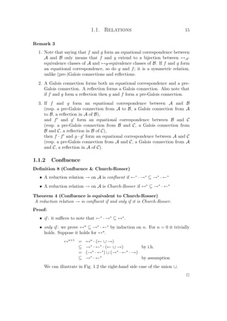
![1.1. Relations 11
1.1 Relations
We take for granted usual notions and results of set theory, such as the empty set
and subsets, the union, intersection and difference of sets, relations, functions,
injectivity, surjectivity, natural numbers. . . (see e.g. [Kri71]). Unless otherwise
stated, relations are binary relations. We denote by |S| the cardinal of a set S.
1.1.1 Definitions notations
Definition 1 (Relations)
• We denote the composition of relations by · , the identity relation by Id,
and the inverse of a relation by −1
, all defined below:
Let R : A −→ B and R : B −→ C.
– Composition
R · R : A −→ C is defined as follows: given M ∈ A and N ∈ C,
M(R · R )N if there exists P ∈ B such that MRP and PR N. Some-
times we also use the notation R ◦ R for R · R .
– Identity
Id[A] : A −→ A is defined as follows:
given M ∈ A and N ∈ A, MIdAN if M = N.
– Inverse
R−1
: B −→ A is defined as follows:
given M ∈ B and N ∈ A, MR−1
N if NRM.
• If D ⊆ A, we write R(D) for {M ∈ B| ∃N ∈ D, NRM}, or equivalently
N∈D{M ∈ B| NRM}. When D is the singleton {M}, we write R(M) for
R({M}).
• Now when A = B we define the relation induced by R through R , written
R [R], as R −1
· R · R : C −→ C.
• We say that a relation R : A −→ B is total if R−1
(B) = A.
• If R : A −→ B and A ⊆ A then R|A : A −→ B is the restriction of R to
A , i.e. those pairs of R whose first components are in A .
• All those notions and notations can be used in the particular case when
R is a function, that is, if ∀M ∈ A, R(M) is of the form {N} (which we
simply write R(M) = N).
• A total function is called a mapping (also called an encoding, a translation
or an interpretation).](https://image.slidesharecdn.com/frenchenglish-150412084606-conversion-gate01/85/French-english-35-320.jpg)
![1.1. Relations 13
Definition 5 (Reduction modulo) Let ∼ be an equivalence relation on a set
A, let → be a reduction relation on A. The reduction relation → modulo ∼ on A,
denoted →∼, is ∼ · → · ∼. It provides a reduction relation on the ∼-equivalence
classes of A. If → is a reduction relation → modulo ∼, → alone is called the
basic reduction relation and denoted →b.1
We now present the notion of simulation. We shall use it for two kinds of
results: confluence (below) and strong normalisation (section 1.2). While sim-
ulation is often presented using an mapping from one calculus to another, we
provide here a useful generalised version for an arbitrary relation between two
calculi.
Definition 6 (Strong and weak simulation)
Let R be a relation between two sets A and B, respectively equipped with the
reduction relations →A and →B.
• →B strongly simulates →A through R if (R−1
· →A) ⊆ (→+
B · R−1
).
In other words, for all M, M ∈ A and for all N ∈ B, if MRN and
M →A M then there is N ∈ B such that M RN and N →+
B N .
Notice that when R is a function, this implies R[→A] ⊆→+
B .
If it is a mapping, then →A ⊆ R−1
[→+
B ].
• →B weakly simulates →A through R if (R−1
· →A) ⊆ (→∗
B · R−1
).
In other words, for all M, M ∈ A and for all N ∈ B, if MRN and
M →A M then there is N ∈ B such that M RN and N →∗
B N .
Notice that when R is a function, this implies R[→A] ⊆→∗
B.
If it is a mapping, then →A ⊆ R−1
[→∗
B].
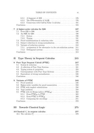
The notions are illustrated in Fig. 1.1.
M
A
R CQ N
B+
M
R CQ N
M
A
R CQ N
B∗
M
R CQ N
Strong simulation Weak simulation
Figure 1.1: Strong and weak simulation
1
This is not a functional notation that only depends on a reduction relation → on ∼-
equivalence classes of A, but a notation that depends on the construction of → as a reduction
relation modulo ∼.](https://image.slidesharecdn.com/frenchenglish-150412084606-conversion-gate01/85/French-english-37-320.jpg)
![14 Chapter 1. Concepts terminology
Remark 2
1. If →B strongly (resp. weakly) simulates →A through R, and if →B⊆→B
and →A⊆→A, then →B strongly (resp. weakly) simulates →A through R.
2. If →B strongly (resp. weakly) simulates →A and →A through R, then it
also strongly (resp. weakly) simulates →A · →A through R.
3. Hence, if →B strongly simulates →A through R, then it also strongly sim-
ulates →+
A through R.
If →B strongly or weakly simulates →A through R, then it also weakly
simulates →+
A and →∗
A through R.
We now define some more elaborate notions based on simulation, such as
equational correspondence [SF93], Galois connection and reflection [MSS86].
Definition 7 (Galois connection, reflection related notions)
Let A and B be sets respectively equipped with the reduction relations →A and
→B. Consider two mappings f : A −→ B and g : B −→ A.
• f and g form an equational correspondence between A and B if the following
holds:
– f[↔A] ⊆↔B
– g[↔B] ⊆↔A
– f · g ⊆↔A
– g · f ⊆↔B
• f and g form a Galois connection from A to B if the following holds:
– →B weakly simulates →A through f
– →A weakly simulates →B through g
– f · g ⊆→∗
A
– g · f ⊆←∗
B
• f and g form a pre-Galois connection from A to B if in the four conditions
above we remove the last one.
• f and g form a reflection in A of B if the following holds:
– →B weakly simulates →A through f
– →A weakly simulates →B through g
– f · g ⊆→∗
A
– g · f = IdB](https://image.slidesharecdn.com/frenchenglish-150412084606-conversion-gate01/85/French-english-38-320.jpg)
![16 Chapter 1. Concepts terminology
∗
11c
c
c
c GGnoo
∗
GG
∗
1
1
1
∗ GG••••••
Figure 1.2: Confluence implies Church-Rosser
Theorem 5 (Confluence by simulation) If f and g form a pre-Galois con-
nection from A to B and →B is confluent, then →A is confluent.
Proof:
←∗
A · →∗
A ⊆ f−1
[←∗
B · →∗
B] weak simulation
⊆ f−1
[→∗
B · ←∗
B] confluence of →B
= f · →∗
B · ←∗
B · f−1
⊆ f · g−1
[→∗
A · ←∗
A] · f−1
weak simulation
= f · g · →∗
A · ←∗
Ag−1
· f−1
weak simulation
⊆ →∗
A · ←∗
A by assumption
This proof can be graphically represented in Fig. 1.3. P
∗
A 66rrrrrrrrr
∗
A{{vvvvvvvvv
f
∗A
$$
f
f
∗ A
ÖÖ
∗
B 66rrrrrrrrr
∗
B{{vvvvvvvvv
∗
B 66rrrrrrrrr
g
∗
B{{vvvvvvvvv
g
g
∗
A
66rrrrrrrrr
∗
A
{{vvvvvvvvv
Figure 1.3: Confluence by simulation
1.1.3 Inference derivations
We take for granted the notion of (labelled) tree, the notions of node, internal
node and leaf, see e.g. [CDG+
97]. In particular, the height of a tree is the length
of its longest branch (e.g. the height of a tree with only one node is 1), and its
size is its number of nodes.
We now introduce the notions of inference structure and derivations. The
former are used to inductively define atomic predicates, which can be seen as](https://image.slidesharecdn.com/frenchenglish-150412084606-conversion-gate01/85/French-english-40-320.jpg)
![18 Chapter 1. Concepts terminology
• We write down derivations by composing with itself the notation with one
horizontal bar that we use for inference steps, as shown in Example 1.
Example 1 (Inference structure derivation) Consider the following in-
ference structure:
d b
c
c b
a d
The following derivation is from {b} to a, has height 3 and size 5.
d b
c b
a
Note the different status of the leaves labelled with b and d, the former being
open and the latter being not.
Definition 11 (Derivability admissibility)
• A tuple of judgements
M1 . . . Mn
M
is derivable in an inference system if there
is a derivation from the set {M1, . . . , Mn} to M.
In this case we write
M1 . . . Mn
========
M
.6
• A tuple of judgements
M1 . . . Mn
M
is admissible in an inference system if for
all derivations of M1 . . . Mn there is a derivation of M.
In this case we write
M1 . . . Mn
· · · · · · · · · ·
M
.
• A tuple of judgements
M1 . . . Mn
M
is height-preserving admissible in an in-
ference system if for all derivations of M1 . . . Mn with heights at most h ∈ N
there exists a derivation of M with height at most h.
In this case we write
M1 . . . Mn
− − − −−
M
.7
6
Note that our notation for derivability, using a double line, is used by some authors for
invertibility. Our notation is based on Kleene’s [Kle52], with the rationale that the double line
evokes several inference steps.
7
The rationale of our notation for height-preserving admissibility is that we can bound the
height of a derivation with fake steps of height-preserving admissibility just by not counting
these steps, since the conclusion in such a step can be derived with a height no greater than
that of some premiss.](https://image.slidesharecdn.com/frenchenglish-150412084606-conversion-gate01/85/French-english-42-320.jpg)
![26 Chapter 1. Concepts terminology
Lemma 17, SN→+
is →+
-patriarchal, so M ∈ SN→+
, and hence
→∗
(M) ⊆ SN→+
.
The statement BN→
n ⊆ BN→+
n can easily be proved by induction on n.
P
Notice that this result enables us to use a stronger induction principle: in order
to prove ∀M ∈ SN→
, P(M), it now suffices to prove
∀M ∈ SN→
, (∀N ∈ →+
(M), P(N)) ⇒ P(M)
This induction principle is called the transitive induction in SN→
.
Theorem 21 (Strong normalisation of disjoint union)
Suppose that (Ai)i∈I is a family of disjoint sets on some index set I, each be-
ing equipped with a reduction relation →i, and consider the reduction relation
→:= i∈I →i on i∈I Ai.
We have i∈I SN→i
⊆ SN→
.
Proof: It suffices to prove that for all j ∈ I, SN→j
⊆ SN→
, which we do by
induction in SN→j
. Assume M ∈ SN→j
and assume the induction hypothesis
→j (M) ⊆ SN→
. We must prove M ∈ SN→
, so it suffices to prove that for all N
such that M → N we have N ∈ SN→
. By definition of the disjoint union, since
M ∈ Ai, all such N are in →j (M) so we can apply the induction hypothesis. P
1.2.2 Termination by simulation
Now that we have established an induction principle on strongly normalising el-
ements, the question arises of how we can prove strong normalisation. In this
subsection we re-establish in our framework the well-known technique of simu-
lation, which can be found for instance in [BN98]. The first technique to prove
that a reduction relation on the set A terminates consists in simulating it (in the
sense of Definition 6) in another set B equipped with its own reduction relation
known to be terminating.
The mapping from A to B is sometimes called the measure function or the
weight function, but Definition 6 generalises the concept to an arbitrary relation
between A and B, not necessarily functional. Similar results are to be found
in [Che04], with the notions of prosimulation, insertion, and repercussion. The
main point here is that the simulation technique is the typical example where the
proof usually starts with “suppose an infinite reduction sequence” and ends with
a contradiction. We show how the use of classical logic is completely unnecessary,
provided that we use a constructive definition of SN such as ours.
Theorem 22 (Strong normalisation by strong simulation) Let R be a re-
lation between A and B, equipped with the reduction relations →A and →B.
If →B strongly simulates →A through R, then R−1
(SN→B
) ⊆ SN→A
.](https://image.slidesharecdn.com/frenchenglish-150412084606-conversion-gate01/85/French-english-50-320.jpg)
![28 Chapter 1. Concepts terminology
Proof: The left-to-right inclusion is an application of Theorem 22: →1 ∪ →2
strongly simulates both →∗
1 · →2 and →1 through Id.
Now we prove the right-to-left inclusion. We first prove the following lemma:
∀M ∈ SN→1
, (→∗
1 · →2)(M) ⊆ SN→1∪→2
⇒ M ∈ SN→1∪→2
We do this by induction in SN→1
, so not only assume (→∗
1 · →2)(M) ⊆ SN→1∪→2
,
but also assume the induction hypothesis:
∀N ∈ →1(M), (→∗
1 · →2)(N) ⊆ SN→1∪→2
⇒ N ∈ SN→1∪→2
.
We want to prove that M ∈ SN→1∪→2
, so it suffices to prove that both
∀N ∈ →2(M), N ∈ SN→1∪→2
and ∀N ∈ →1(M), N ∈ SN→1∪→2
. The former case
is a particular case of the first hypothesis. The latter case would be provided
by the second hypothesis (the induction hypothesis) if only we could prove that
(→∗
1 ·→2)(N) ⊆ SN→1∪→2
. But this is true because (→∗
1 ·→2)(N) ⊆ (→∗
1 ·→2)(M)
and the first hypothesis reapplies.
Now we prove
∀M ∈ SN→∗
1·→2
, M ∈ SN→1
⇒ M ∈ SN→1∪→2
We do this by induction in SN→∗
1·→2
, so not only assume M ∈ SN→1
, but also as-
sume the induction hypothesis ∀N ∈ (→∗
1 ·→2)(M), N ∈ SN→1
⇒ N ∈ SN→1∪→2
.
Now we can combine those two hypotheses, because we know that SN→1
is stable
under →2: since M ∈ SN→1
, we have (→∗
1 · →2)(M) ⊆ SN→1
, so that the induc-
tion hypothesis can be simplified in ∀N ∈ (→∗
1 · →2)(M), N ∈ SN→1∪→2
.
This gives us exactly the conditions to apply the above lemma to M. P
Definition 17 (Lexicographic reduction) Let A1, . . . , An be sets,
respectively equipped with the reduction relations →A1 , . . . , →An .
For 1 ≤ i ≤ n, let →i be the reduction relation on A1 × · · · × An defined as
follows:
(M1, . . . , Mn) →i (N1, . . . , Nn)
if Mi →Ai
Ni and for all 1 ≤ j i, Mj = Nj and for all i j ≤ n, Nj ∈ SN→Aj .
We define the lexicographic reduction
→lex=
1≤i≤n
→i
We sometimes write →lexx for →lex
+
, i.e. the transitive closure of →lex.9
Corollary 24 (Lexicographic termination 1)
SN→A1 × · · · × SN→An ⊆ SN→lex
In particular, if →Ai
is terminating on Ai for all 1 ≤ i ≤ n, then →lex is termi-
nating on A1 × · · · × An.
9
This is the traditional lexicographic order, see e.g. [Ter03].](https://image.slidesharecdn.com/frenchenglish-150412084606-conversion-gate01/85/French-english-52-320.jpg)
![30 Chapter 1. Concepts terminology
M
A∗
R CQ N ∈ SN→B
B∗
M1
A
R CQ N1
B+
M1
A∗
R CQ N1
B∗
M2
A
R CQ N2
B+
Mi
A∗
R CQ Ni
Mi+j
A∗
R
PXmmmmmmmmmmmmmmm
mmmmmmmmmmmmmmm R
Vdxxxxxxxxxxxxxxxxxxxxx
xxxxxxxxxxxxxxxxxxxxx
Figure 1.6: Deriving strong normalisation by lexicographic simulation
1.2.4 Multi-set termination
Now we define the notions of multi-sets their reductions [DM79, BN98]. We
constructively prove their termination. Classical proofs of the result can also be
found in [Ter03].
Definition 18 (Multi-Sets)
• Given a set A, a multi-set of A is a total function from A to the natural
numbers such that only a finite subset of elements are not mapped to 0.
• Note that for two multi-sets f and g, the function f + g mapping any
element M of A to f(M) + g(M) is still a multi-set of A and is called
the (multi-set) union of f and g. We also define the multi-set f g as the
function mapping each element M ∈ A to max(f(M) − g(M), 0).
• We define the multi-set {{N1, . . . , Nn}} as f1 + · · · + fn, where for all
1 ≤ i ≤ n, fi maps Ni to 1 and every other element to 0.
• We abusively write M ∈ f if f(M) = 0.](https://image.slidesharecdn.com/frenchenglish-150412084606-conversion-gate01/85/French-english-54-320.jpg)
![1.2. A constructive theory of normalisation 31
Definition 19 (Multi-Set reduction relation) Given → is a reduction rela-
tion on A, we define the multi-set reduction as follows:
if f and g are multi-sets of A, we say that f →mul g if there is a M in A such
that
f(M) = g(M) + 1
∀N ∈ A, f(N) g(N) ⇒ M → N
We sometimes write →mull for →mul
+
, i.e. the transitive closure of →mul.10
Example 2 (Multi-set reduction) Considering multi-sets of natural numbers,
for which the reduction relation is , we have for instance
{{5, 7, 3, 5, 1, 3}}mul{{4, 3, 1, 7, 3, 5, 1, 3}}. In this case, the element M is 5, and
an occurrence has been “replaced” by 4, 3, 1, which are all smaller than 5.
In what follows we always assume that A is a set with a reduction relation →.
Lemma 27 If f1, . . . , fn, g are multi-sets of A and f1 +· · ·+fn →mul g then there
is 1 ≤ i ≤ n and a multi-set fi such that fi →mul fi and
f1 + · · · + fi−1 + fi + fi+1 + · · · + fn = g.
Proof: We know that there is a M in A such that
f1(M) + · · · + fn(M) = g(M) + 1
∀N ∈ A, f1(N) + · · · + fn(N) g(N) ⇒ M → N
An easy lexicographic induction on two natural numbers p and q shows that if
p + q 0 then p 0 or q 0. By induction on the natural number n, we
extend this result: if p1 + · · · + pn 0 then ∃i, pi 0. We apply this result on
f1(M) + · · · + fn(M) and get some fi(M) 0. Obviously there is a unique fi
such that f1 + · · · + fi−1 + fi + fi+1 + · · · + fn = g, and we also get fi →mul fi. P
Definition 20 (Sets of multi-sets) Given two sets N and N of multi-sets, we
define N + N as {f + g | f ∈ N, g ∈ N }.
We define for every M in A its relative multi-sets as all the multi-sets f of A
such that if N ∈ f then M →∗
N. We denote the set of relative multi-sets as
MM .
Remark 28 Notice that for any M ∈ A, MM is stable under →mul.
Lemma 29 For all M1, . . . , Mn in A, if MM1 ∪ . . . ∪ MMn ⊆ SN→mul
then MM1 + · · · + MMn ⊆ SN→mul
.
Proof: Let W be the relation between MM1 +· · ·+MMn and MM1 ×· · ·×MMn
defined as: f1 + · · · + fnW(f1, . . . , fn) for all f1, . . . , fn in MM1 × · · · × MMn .
10
This is the traditional multi-set order, see e.g. [Ter03].](https://image.slidesharecdn.com/frenchenglish-150412084606-conversion-gate01/85/French-english-55-320.jpg)
![1.3. Higher-Order Calculi (HOC) 33
1.3 Higher-Order Calculi (HOC)
In this section we introduce higher-order calculi, in which the set A is recursively
defined by a term syntax possibly involving variable binding and the reduction
relation → is defined as a rewrite system. This section is intended to capture all
the formalisms introduced in the rest of this thesis, which are quite numerous.
1.3.1 Introduction and literature
There are several ways to express higher-order calculi in a generic way, among
which Higher-Order Systems (HRS) [Nip91], Combinatory Reduction Systems
(CRS) [Klo80], Expression Reduction Systems (ERS) [Kha90], Interaction Sys-
tems (IS) [AL94], etc. These formalisms are presented in particular in [Ter03]
with a comparative approach.
Here we choose a presentation of higher-order calculi of which traditional
presentations of many calculi are direct instances. In this presentation, higher-
order terms can be seen as those of HRS, i.e. the η-long β-normal forms of the
simply-typed λ-calculus [Bar84] extended with constants (representing term con-
structors). Types are here called syntactic categories to avoid confusion with
systems presented later.
The notion of reduction is given by rewriting. However, unlike the aforemen-
tioned formalisms, rewrite systems are considered not at the object-level but at
the meta-level as a way to define a (reduction) relation (just like we can define a
function by a set of equations treating different cases for its argument).
We thus use in rewrite systems the same meta-variables for terms as in the rest
of the dissertation, i.e. those variables of the meta-level that we use to quantify
over terms in statements and proofs. Meta-variables are convenient to describe
higher-order grammars in BNF-format and allow the presentation of rewrite sys-
tems in a traditional way. They are similar to those of CRS and even more
similar to those of ERS and IS (since they have no arity and are not applied).
These formalisms internalise parts of the meta-level (such as rewrite systems with
meta-variables) into the object-level.
The meta-level language for describing higher-order calculi can actually be
considered on its own as an object, and this is for example what we do in sec-
tion 1.3.3 to state our conventions for dropping the side-conditions that are needed
in first-order logic to deal with α-conversion and avoid variable capture and lib-
eration.
Particular definitions of reduction relations can thus be encoded at the object-
level in the formalisms mentioned earlier, so that we can use established results
such as confluence of orthogonal systems. Rewriting in IS is constrained by
the notions of constructor and destructor (here we call term constructor any
constant) and that in ERS is more general, but it is into HRS that we explicitly
give an encoding (section 1.3.4), both because we want to use its intrinsic typing](https://image.slidesharecdn.com/frenchenglish-150412084606-conversion-gate01/85/French-english-57-320.jpg)
![1.3. Higher-Order Calculi (HOC) 35
– a set of elements called term constructors (or just constructors), de-
noted c C.
A basic syntactic category T with variables and such that for no C1, . . . , Cn
there is a term constructor c C1 → · · · → Cn → T is called a variable category.
We sometimes write f for either a variable or a term constructor. The arity
of f C is arity(C).
The aforementioned sets of variables are assumed to be pairwise disjoint. We
also fix a total order on the set of all variables.
Definition 23 (Syntactic terms of HOC)
• In such an HOC, the syntactic terms of a syntactic category are trees whose
nodes are labelled with either variables, term constructors or a dot with
a bracketed variable, and respecting the syntactic categories in the sense
specified by the following two rules:
For each variable or term constructor f C1 → · · · → Cn → T
(with n ≥ 0 and T being a basic syntactic category),
(Si Ci)1≤i≤n
f(S1, . . . , Sn) T
For each variable x C1,
S C2
[x].S C1 → C2
• The height and size of a syntactic term are its height and size as a tree. The
notion of sub-tree (resp. strict sub-tree) provides the notion of sub-syntactic
term (resp. strict sub-syntactic term). If S is a sub-syntactic term (resp.
strict sub-syntactic term) of S we write S S (resp. S S ), and we
write for −1
(resp. for −1
).
• The terminating relation provides a notion of induction on syntactic
terms.
• We abbreviate f() as f for a variable or term constructor f T .
• The notion of equality between syntactic terms is sometimes called syntactic
equality.
Example 3 (λ-calculus as an HOC) We can express the syntax of λ-calculus
as an HOC. There is one basic syntactic category T with variables, and there are
two term constructors: the abstraction λ : (T → T ) → T and the application,
of the syntactic category T → T → T .](https://image.slidesharecdn.com/frenchenglish-150412084606-conversion-gate01/85/French-english-59-320.jpg)
![36 Chapter 1. Concepts terminology
It will often be necessary to rename variables, and a elegant way of doing it
is by swapping two variables, a notion borrowed from nominal logic [Pit03].
Definition 24 (Swapping) The swapping of two variables x and y in a syntac-
tic term S is defined by induction on S, using the swapping of two variables x
and y on a variable z:
(x y)x := y
(x y)y := x
(x y)z := z z = x, z = y
(x y)(z(S1, . . . , Sn)) := ((x y)z)((x y)S1, . . . , (x y)Sn)
(x y)(c(S1, . . . , Sn)) := c((x y)S1, . . . , (x y)Sn)
(x y)([z].S) := [(x y)z].(x y)S
Remark 32 Swapping preserves the height and size of syntactic terms.
Definition 25 (Syntactic terms relations) A relation R between syntac-
tic terms respects syntactic categories if whenever SRS then S and S belong to
the same syntactic category.
Definition 26 (Free variables) The set of free C-variables of a syntactic term
S, denoted FVC(S) is defined inductively as follows:
FVC(x(S1, . . . , Sn)) := {x} ∪ 1≤i≤n FVC(Si) if x C
FVC(x(S1, . . . , Sn)) := 1≤i≤n FVC(Si) if not
FVC(c(S1, . . . , Sn)) := 1≤i≤n FVC(Si)
FVC([x].S) := FVC(S) x
We also write FV(S) for C FVC(S) (C ranging over categories with variables) or
when C is unique or clear from context.
The construct [x].S gives a mechanism for binding and induces a notion of α-
equivalence, for which we follow Kahrs’ definition [Kah92]. Again, this definition
is an example of an inference structure.
Definition 27 (α-equivalence)
• Two syntactic terms S, S are α-equivalent, denoted S=αS , if the judgement
S =α S is derivable in the following inference structure for judgements
of the form Γ S =α S or Γ x − y (where Γ is a list of pairs of variables
written x − y ):](https://image.slidesharecdn.com/frenchenglish-150412084606-conversion-gate01/85/French-english-60-320.jpg)
![1.3. Higher-Order Calculi (HOC) 37
x − x Γ, x − y x − y
Γ x − y
x = x ∧ y = y
Γ, x − y x − y
Γ x − y (Γ Si =α Si)1≤i≤n
Γ x(S1, . . . , Sn) =α y(S1, . . . , Sn)
(Γ Si =α Si)1≤i≤n
Γ c(S1, . . . , Sn) =α c(S1, . . . , Sn)
Γ, x − y S1 =α S2
x C ∧ y C
Γ [x].S1 =α [y].S2
• A relation R between syntactic terms is compatible with α-equivalence if
(=α · R · =α) ⊆ R.
• A function f from syntactic terms to a set A is compatible with α-equivalence
if α-equivalent terms are mapped to the same element of A.
Remark 33
1. If x ∈ FV(S) then [y].S =α [x].(x y)S.
2. α-equivalence is an equivalence relation that respects syntactic categories.
Definition 28 (Terms of HOC)
• The terms of HOC are simply the α-equivalence classes of syntactic terms.11
• We now introduce notations whose meanings are defined inductively as
terms:
– x.M denotes the α-equivalence class of [x].S if M denotes the α-
equivalence class of S,
– f(M1, . . . , Mn) denotes the α-equivalence class of f(S1, . . . , Sn) if each
Mi denotes the α-equivalence class of Si and f is a variable or a term
constructor. (Again we abbreviate f() as f for a variable or term
constructor f T .)
A term x.M is called abstraction or binder on x with scope M.
11
The terms of HOC can be seen as the η-long β-normal forms of the simply-typed λ-calculus
(extended with constants corresponding to term constructors), i.e. as the terms of HRS, in
effect. (Note however in Definition 22 that we can prevent some syntactic categories from
being inhabited by variables.)](https://image.slidesharecdn.com/frenchenglish-150412084606-conversion-gate01/85/French-english-61-320.jpg)
![1.3. Higher-Order Calculi (HOC) 41
• to denote a binder of the object level,
• to denote a construction in which some variable name does not matter, as
for the (implicit) substitution N
x M that we define in this section.
Both kinds of bindings introduce the problem of variable capture and liberation.
We might want to write for instance
• a rule like η-reduction in λ-calculus: λx.M x → M, or the propagation of
an explicit substitution through an abstraction in the λx-calculus [BR95]:
P/y λx.M → λx. P/y M (all bindings from the object-level)
• the substitution lemma P
y
N
x M = {P
y}N
x
P
y M (all bindings
from the meta-level)
• the case of the abstraction for the definition of (implicit) substitution:
P
y (x.M) = x. P
y M (interaction between object-level binding and
meta-level binding)
The side-conditions avoiding variable capture and liberation are x ∈ FV(M) for
η-reduction, and x ∈ FV(P) and x = y for the rule of λx, the substitution lemma,
and the definition of implicit substitution. In all cases we want a safe way to drop
these side-conditions, because they can be mechanically recovered just by looking
at the above expressions, and this is the main point of this section. But in order to
define this mechanical process, information about the intended variable bindings
must be available, so we slightly enrich the sorting of multi-sorted first-order logic
so that it bears this information.
The grammar for syntactic categories of the meta-level must cover every kind
of notation used in this dissertation. First-order notations are standard to deal
with, but expressions of the meta-level might intend not only unary bindings
(as in the example of the substitution) but also n-ary bindings, i.e. bindings of
several variables in one construct. For example in Chapter 5 we use lists. Lists
can be used as binders in a notation of λ-calculus like λΠ.M that stands for
λx1. . . . .λxn.M if Π is the list x1, . . . , xn. In this case writing N
x (λΠ.M) =
λΠ. N
x M should generate the side-conditions Dom(Π) ∩ FV(N) = ∅ and
x ∈ Dom(Π), which are more complex than the side-conditions of the previous
examples.
Definition 35 (Syntactic categories of the meta-level)
The meta-level uses the basic syntactic categories of the object-level but new ones
can also be used, given in a set SCM
. Syntactic categories of the meta-level are
given by the following grammar:
S ::= U ∈ SCM
| B | P](https://image.slidesharecdn.com/frenchenglish-150412084606-conversion-gate01/85/French-english-65-320.jpg)
![44 Chapter 1. Concepts terminology
Example 5 (Constructions)
• In the meta-language we often use notions from set theory, for instance
we have the constructions FVC
... T SetsC for each T. We also have
constructions ∅
... SetsC and ∪, ∩
... SetsC SetsC SetsC that we use as
usual as an infix notation, as well as set difference denoted .
• We have also used Support
... VC SetsC and Support
... ListsC SetsC and
the swapping (_ _)_
... VC VC T T.
Generalised swapping can apply to expressions of other syntactic categories:
we general say that an expression E can be subject to the swapping operator
if it makes sense to write (X Y)E.
• Note that the notation _._ can itself be considered a construction of
B T (B × T) with a particular binding behaviour. On the con-
trary, the notation [_]._ for syntactic terms, that has no intrinsic notion
of binding, can be seen as a construction of VC STC STC →C if STC
is the syntactic category in SCM
of the expressions representing syntactic
terms of C. No side-condition avoiding variable capture and liberation will
then be produced, since the represented objects are syntactic terms and not
equivalence classes of them.
• For each syntactic category C of the object level and each syntactic category
P, we have an construction called substitution in
(VC × P) C†
P.
The construction of substitution, when applied to two arguments X.E and
E , is denoted E
X E.
• We have mentioned that we sometimes use lists, such as in Π.M, and we
sometimes write x1. . . . .xn for Π = (xi)1≤i≤n.
We now describe how we define HOC in BNF-format, noting that a connection
between BNF-definitions and ERS has been studied in [Kha90].
Definition 39 (BNF-definitions) We shall often give the grammar of an HOC
in BNF-format, by giving for each syntactic category T a structure like the fol-
lowing one:
MT , NT , . . . ::= XT (
−−→
X1C1
.M1T1
, . . . ,
−−−→
XmCm
.MmTm
) | . . .
| cT (
−−→
X1C1
.M1T1
, . . . ,
−−→
XnCn
.MnTn
) | . . .
where
• MT , NT , . . . is a scheme describing the meta-variables of T ,](https://image.slidesharecdn.com/frenchenglish-150412084606-conversion-gate01/85/French-english-68-320.jpg)
![1.3. Higher-Order Calculi (HOC) 45
• XT (
−−→
X1C1
.M1T1
, . . . ,
−−−→
XmCm
.MmTm
) | . . . is a scheme describing the constructs
with the meta-variables XT
... VC1 →···→Cm →T (with, for all 1 ≤ i ≤ m,
Ci = Ci,1 → · · · → Ci,pi
→ Ti, and
−−→
XiCi
. representing a series of bindings on
(Xi,j
... VCi,j
)1≤j≤pi
, and MiTi
being a meta-variable of Ti),
• cT (
−−→
X1C1
.M1T1
, . . . ,
−−→
XnCn
.MnTn
) | . . . is a scheme describing the constructs
with the term constructors cT C1 → · · · → Cn → T (with, for all
1 ≤ i ≤ n, Ci = Ci,1 → · · · → Ci,pi
→ Ti , and
−−→
XiCi
. representing a se-
ries of bindings on (Xi,j
... VCi,j
)1≤j≤pi
, and MiTi
being a meta-variable of
Ti ).
Either of the last two schemes can be absent when the sets of such variables
or term constructors are empty (e.g. variable-free syntactic categories).
All isomorphic notations are acceptable in the definition of HOC, as long as the
binders and their scopes are specified. Traditional notations will thus be allowed.
For instance we can write a term construct as N/x M instead of expsub(x.M, N)
for explicit substitutions such as those of λx [BR95]. More generally, when a term
constructor corresponds, in some sense, to a construction, we tend to use angled
brackets for the term constructor and braces for the construction (as in the case
of explicit and implicit substitutions).
Example 6 (BNF-definition of λ-calculus) We re-express in BNF-format the
definition of the syntax of λ-calculus from Example 3:
M, N ::= x | λx.M | M N
But we can also define the notation λΠ.M if Π is a list of variables, where
λx1, . . . , xn.M abbreviates λx1. . . . .λxn.M.
Note that for a variable category T of order 0, the meta-variables for terms
in T are abusively taken to be the same as meta-variables for variables in VT . In
BNF-definitions we thus often omit lines such as
M ::= X
and we use X everywhere instead of M, as we illustrate with the following example.
Example 7 (BNF-definition of λx) We can express in BNF-format the defi-
nition of the syntax of the calculus with explicit substitutions λx by [BR95].16
Instead of
U, V ::= x
M, N ::= var(U) | λx.M | M N | N/x M
16
As discussed in Chapter 4, this presentation of λx is one among others.](https://image.slidesharecdn.com/frenchenglish-150412084606-conversion-gate01/85/French-english-69-320.jpg)
![46 Chapter 1. Concepts terminology
we can more simply write
M, N ::= var(x) | λx.M | M N | N/x M
We also abusively write
M, N ::= x | λx.M | M N | N/x M
if it is clear from context that variables form a syntactic category of their own.
As mentioned in the introduction of this chapter, we now develop the ideas
of Barendregt’s convention by giving a mechanical way to recover, just from the
expressions we write to denote terms, the side-conditions that are needed to
avoid variable capture and liberation. We shall then be able to safely drop those
side-conditions throughout the rest of this dissertation.
Nominal logic [Pit03] might be a way of implementing the reasonings that use
such conventions in first-order logic.
The idea is very close to the notion of parameter path of SERS [BKR00]
(a particular notion of ERS): given a finite set of expressions (Ei)1≤i≤n with
occurrences of a particular meta-variable for terms M, [BKR00] forbids M to be
instantiated with a term that contains a variable that is bound by the parameter
path of one occurrence and not by that of another occurrence.
Here we bypass the notion of instance but instead produce the side-conditions,
directly expressed in the meta-language, that avoid variable capture and liber-
ation. For this we define a set-theoretic expression of the meta-language that
represents the set of variables that are allowed to occur freely in the term rep-
resented by M but that are bound outside by abstractions having M in their
scopes.
We first need to define what the meta-variables of an expression are. For
that we use set theoretic notions (at the meta-meta-level), which we need to
distinguish from the set-theoretic constructions of the meta-level. Hence we write
[], , , E, [. . .] for the former and ∅, ∪, ∩, ∈, {. . .} for the latter. For instance, if
F is the set [E1, . . . , En] of expressions denoting sets, then F stands for the
expression E1 ∪. . .∪En (for any particular order) while F does not make sense
(the (Ei)1≤i≤n are not sets but expressions).](https://image.slidesharecdn.com/frenchenglish-150412084606-conversion-gate01/85/French-english-70-320.jpg)
![1.3. Higher-Order Calculi (HOC) 47
Definition 40 (Meta-variables of an expression) We define the meta-
variables for terms variables MV(E) of an expression E by induction on E:
MV(M) := [M] if M
... T
MV(M) := [] if not
MV(E .E) := MV(E)
MV(X(E1, . . . , En)) := [X] 1≤i≤n MV(Ei)
MV(c(E1, . . . , En)) := 1≤i≤n MV(Ei)
MV(d(E1, . . . , En)) := 1≤i≤n MV(Ei)
where X, c and d are respectively a meta-variable
of some VC, a term constructor and a construction
Definition 41 (Allowed variables)
• The expression of allowed variables in a meta-variable M E MV(E), denoted
AVeM(E), is an expression defined by induction on E:
AVeM(M) := ∅
AVeM(E .E) := AVeM(E) ∪ Support(E )
AVeM(M(E1, . . . , En)) := ∅
AVeM(X(E1, . . . , En)) := [AVeM(Ei) | M ∈ MV(Ei)] if X = M
AVeM(c(E1, . . . , En)) := [AVeM(Ei) | M ∈ MV(Ei)]
AVeM(d(E1, . . . , En)) := [AVeM(Ei) | M ∈ MV(Ei)]
where X, c and d respectively stand for a meta-variable
of some VC, a term constructor and a construction
• Suppose every construct E1.E2 in an expression E are such that E1 = X
... VC.
The set of allowed meta-variables in a meta-variable M E MV(E), denoted
AVsM(E), is the set of meta-variables defined by induction on E as follows:
AVsM(M) := []
AVsM(X.E) := AVsM(E) [X]
AVsM(M(E1, . . . , En)) := []
AVsM(X(E1, . . . , En)) := [AVsM(Ei) | M ∈ MV(Ei)] if X = M
AVsM(c(E1, . . . , En)) := [AVsM(Ei) | M ∈ MV(Ei)]
AVsM(d(E1, . . . , En)) := [AVsM(Ei) | M ∈ MV(Ei)]
where X, c and d respectively stand for a meta-variable
of some VC, a term constructor and a construction
Definition 42 (Generation of side-conditions) We define the side-
conditions against capture and liberation of a finite set of expressions [E1, . . . , En].
These are expressed directly in the meta-language and defined by use of a similar
notion for a single expression E:](https://image.slidesharecdn.com/frenchenglish-150412084606-conversion-gate01/85/French-english-71-320.jpg)
![48 Chapter 1. Concepts terminology
• For E = M, there is no side-condition.
• For E = E .E , the side-conditions are those of E and those of E , plus
Support(E ) ∩ AVeM(E ) = ∅
for each meta-variable M ∈ MV(E ).
• For E = c(E1, . . . , En) or E = d(E1, . . . , En) (where c and d respectively
stand for a term constructor and an construction), the side-conditions are
those of {E1, . . . , En}.
• For E = X(E1, . . . , En) (where X
... VC for some C), the side-conditions are
those of [E1, . . . , En], plus
[AVeX(Ei) | X ∈ MV(Ei)] = ∅
• The side-conditions of [E1, . . . , En] are:
for each meta-variable M ∈ 1≤i≤n MV(Ei),
F F ∩ FV(M) = ∅
writing F for the set of expressions [AVeM(Ei) | M ∈ MV(Ei)],
as well as the side-conditions produced by each Ei.
Remark 39 Note that the meta-variables that appear in the side-conditions
produced by the process above can all be subject to the swapping operator.
Example 8 (Side-conditions against variable capture and liberation)
• AVeM (c(x.y.M, Π.M)) is the expression
(((∅ ∪ Support(y)) ∪ Support(x)) ∩ Support(Π))
and because the meta-level uses first-order logic with set theory, this is
therein equal to {x, y} ∩ Support(Π).
The side-conditions are equal, after a similar set-theoretic simplification at
the meta-level, to (({y, x}∪Support(Π))({y, x}∩Support(Π)))∩FV(M) = ∅
and x = y.
If Support(Π) = {y, z} then AVeM (c(x.y.M, Π.M)) = {y} and the first side-
condition becomes {x, z} ∩ FV(M) = ∅, i.e. x ∈ FV(M) and z ∈ FV(M).
• Note that the expression λx.λx.M of λ-calculus, although we are allowed
to write it, produces the unsatisfiable side-condition x = x. To denote
the α-equivalence class of λ[x].λ[x].M, we can use λy.λx.M with the side-
condition y ∈ FV(M).](https://image.slidesharecdn.com/frenchenglish-150412084606-conversion-gate01/85/French-english-72-320.jpg)
![1.3. Higher-Order Calculi (HOC) 53
• As an example of a (non-reductive) term rewrite system we can give β-
expansion:
N
x M −→ (λx.M) N
Analysing how the rule applies to some term is not straightforward because
of the implicit substitution.
• As an example of the most general notion of rewrite system we can give a
rule that eliminates several occurrences of an element in a multi-set:
Γ + {{A, A}} −→ Γ + {{A}}
Note that Γ+{{A, A}} is not a term, it could be for instance {{B, A, C, D, A}}.
Definition 47 (Root reduction redex)
• The relation denoted by a term rewrite system R is written
r o o t
−→R at the
meta-level, and its contextual closure is written −→R (for cc
r o o t
−→R ). As-
suming M −→R N implies a root reduction inside M and a derivation
for the contextual closure, on which we can do inductions. We call such
an induction induction on (the derivation of) the reduction step, with root
reduction as the base case.
• A R-redex of a term (or simply redex when the term rewrite system R is
clear from context) is a sub-term that is
r o o t
−→R -reducible.
• We simply say R-normal form (resp. R-reducible form) for −→R -normal
form (resp. −→R -reducible form).
Definition 48 (Strongly weakly normalising systems) A term rewrite sys-
tem R is strongly normalising/terminating or weakly normalising on a set of terms
T (or it terminates on T ) if −→R is.
If we do not specify T , it means that we take T = A.
As we have already said in the introduction of this section, particular re-
duction relations could be given by HRS (rather than by rewrite systems at the
meta-level as defined above). Such an alternative definition is useful to use estab-
lished theorems of HRS such as confluence of orthogonal systems. We refer the
reader to [Ter03] for the definition of a HRS and the reduction relation induced
by it. However the HRS have to be given in each case, unless the work is fac-
torised by analysing the way that the meta-level defines the reduction relations.
Indeed, in the same way as we could generically produce a theorem of the meta-
level from assumptions about the meta-level (Lemma 42), we can also generically
produce a definition of the meta-level from assumptions about the meta-level.
These assumptions are that the reduction relation is given by an atomic rewrite
systems.
We start by defining the η-long form of a variable as follows](https://image.slidesharecdn.com/frenchenglish-150412084606-conversion-gate01/85/French-english-77-320.jpg)
![1.3. Higher-Order Calculi (HOC) 55
Remark 45 Consider an atomic rewrite system R. The proposition
“The reduction relation −→R between terms is equal to the one generated by a
corresponding HRS.”
is a theorem of the meta-level.
Remark 46 We sometimes use the terminology “system” and “rule” directly at
the meta-level, to which we now come back.
1.3.5 Induction principles with HOC
Lemma 47 If R is a reduction system on terms of an HOC, then
SN−→R ∪
= SN−→R
.
Proof: This is a typical theorem that is usually proved classically (using for
instance the postponing technique [Ter03]). We prove it constructively here. The
left-to-right inclusion is trivial, by Lemma 20. Now for the other direction, first
notice that SN = A. Because of the definition of a contextual closure, −→R
strongly simulates −→R through . Also, it weakly simulates through , so we
may apply Corollary 26 and get ∀N ∈ SN→R
, ∀M ∈ A, M N ⇒ M ∈ SN→R∪
.
In particular, ∀N ∈ SN→R
, M ∈ SN→R∪
. P
Notice that this result enables us to use a stronger induction principle: in
order to prove ∀M ∈ SN−→R
, P(M), it now suffices to prove
∀M ∈ SN−→R
, (∀N ∈ A, (M−→+
R N ∨ N M) ⇒ P(N)) ⇒ P(M)
This induction principle is called the transitive induction in SNR
with sub-terms
and is used in the following sections.
We briefly recall the various induction principles:
In order to prove ∀M ∈ SN−→R
, P(M), it suffices to prove
• ∀M ∈ A, (∀N ∈ A, (M −→R N) ⇒ P(N)) ⇒ P(M)
(raw induction in SNR
), or just
• ∀M ∈ SN−→R
, (∀N ∈ A, (M −→R N) ⇒ P(N)) ⇒ P(M)
(induction in SNR
), or just
• ∀M ∈ SN−→R
, (∀N ∈ A, (M−→+
R N) ⇒ P(N)) ⇒ P(M)
(transitive induction in SNR
), or even
• ∀M ∈ SN−→R
, (∀N ∈ A, (M−→+
R N ∨ N M) ⇒ P(N)) ⇒ P(M)
(transitive induction in SNR
with sub-terms)
Definition 51 SNR
henceforth denotes SN−→R ∪
= SN−→R
.](https://image.slidesharecdn.com/frenchenglish-150412084606-conversion-gate01/85/French-english-79-320.jpg)
![56 Chapter 1. Concepts terminology
1.4 Termination by Recursive Path Ordering
Having defined the notion of HOC, we now give another technique to prove ter-
mination: the Recursive Path Orderings (RPO) [Der82]. In this section we define
the concepts for first-order terms only, i.e. those terms built with constructors
whose syntactic categories are of order 1 (in other word, there is no variable bind-
ing). The technique of RPO will still be relevant for HOC in general, which can
all be turned into first-order calculi by erasing all bindings and replacing every
bound variable by a common constructor of arity 0, say (pronounced blob).
Such an encoding loses the information about the higher-order features of the
calculus but will work for our purposes. The RPO technique could equivalently
be defined for HOC in general, by embedding the erasure of bound variables into
the definitions,20
but the literature usually makes the encoding explicit, as we
shall do as well.
Definition 52 (Path Orderings) Consider a terminating and transitive re-
duction relation on term constructors of the HOC. In the context of path
orderings this will be called the precedence relation.
• Suppose that each term constructor is labelled with a status lex or mul.
The Recursive Path Ordering (RPO) [Der82], noted , is the relation on
terms defined inductively21
by the following rules:
c(M1, . . . , Mn)Mi
MiM
c(M1, . . . , Mn)M
(c(M1, . . . , Mn)Ni)1≤i≤n
c d
c(M1, . . . , Mn)d(N1, . . . , Nm)
if c has status lex
(M1, . . . , Mn)lexx(N1, . . . , Nn) (c(M1, . . . , Mn)Ni)1≤i≤n
c(M1, . . . , Mn)c(N1, . . . , Nn)
if c has status mul
{{M1, . . . , Mn}}mull{{N1, . . . , Nm}}
c(M1, . . . , Mn)c(N1, . . . , Nm)
20
This is clearly quite different from (and much weaker than) Jouannaud and Rubio’s higher-
order RPO [JR99], which takes the higher-order features into account, by including in the
technique the termination of the simply-typed λ-calculus.
21
Note that because of the reference to the multi-set reduction and the lexicographic reduc-
tion, the above rules do not form a proper inductive definition. However, we can label with
integers and define k by induction on k using the rules. Then it suffices to take = k k.
See [Ter03] for a discussion on this.](https://image.slidesharecdn.com/frenchenglish-150412084606-conversion-gate01/85/French-english-80-320.jpg)
![Conclusion 57
where d and c are term constructors with arities m and n, respectively, and
M, the Mi, and the Nj are terms.
• The Lexicographic Path Ordering (LPO) [KL80] is the RPO obtained by
giving the label lex to all term constructors.
• The Multi-set Path Ordering (MPO) is the RPO obtained by giving the
label mul to all term constructors.
Remark 48
1. If s t then st, which we call the sub-term property of .
2. The relation is transitive and context-closed.
Theorem 49 (Termination of RPO) If terminates on the set of term con-
structors, then terminates on the set of terms.
Proof: See e.g. [Ter03] for a classical proof. P
Conclusion
In this chapter we have established the notations, the terminology and the basic
concepts that are used in the rest of this dissertation. We have presented a
constructive theory of normalisation and induction based on an approach that
relies on second-order quantification rather than classical logic. We have re-
established a few normalisation results in this framework, including the simulation
technique and a few variants.
We have presented higher-order calculi (HOC), i.e. calculi involving variable
binding. Variable capture an liberation is avoided by the use of side-conditions
that we often not write explicitly, but instead we described how they can be
recovered mechanically from the expressions that we use to denote terms, building
on the principles behind Barendregt’s convention. For that we needed to formalise
the meta-level. This step back could be avoided by encoding parts of the meta-
level into the object-level, such as introducing meta-variables in the syntax of
higher-order calculi. This is the approach of CRS, ERS and IS. However, the
extent of meta-level encoded in the object-level might not feature any notions of
variable binding other than the object-level bindings (and possibly the bindings
of implicit substitutions). Here we wanted to define a notion of expression that
can feature any object-level and meta-level bindings.](https://image.slidesharecdn.com/frenchenglish-150412084606-conversion-gate01/85/French-english-81-320.jpg)


![Chapter 2
Natural deduction sequent
calculus
In this chapter we introduce the concepts common to all chapters of Part I,
which investigates intuitionistic implicational logic, i.e. intuitionistic logic with
implication as the only logical connective. We start by formalising, in a more
generic framework, a generalisation of the aforementioned concepts (also used in
Part III which tackles classical logic), such as the notions of logical systems and
typing systems, proof-terms, etc.
The paradigm of the Curry-Howard correspondence, which relates logical sys-
tems and typing systems, is then illustrated not only by (intuitionistic implica-
tional) natural deduction and the simply-typed λ-calculus [How80], but also by
a typed HOC corresponding to the (intuitionistic implicational) sequent calculus
G3ii [Kle52]. We conclude the chapter by recalling traditional encodings from
one to the other, originating from works by Gentzen [Gen35] and Prawitz [Pra65]
but here presented by type-preserving translations of proof-terms (as in e.g.
[Zuc74, DP99b]).
The main purpose of this chapter is to make the dissertation self-contained,
but most concepts formalised therein correspond, in each particular framework
treated in this dissertation, to the standard ones, so the reader may safely skip
them (note however some notions that are new, such as being logically principal
—Definition 57, and term-irrelevant admissibility —Definition 65).
2.1 Logical systems implicational intuitionistic
logic
We first introduce general notions related to logical systems. The syntax of logical
systems is based on HOC as described in Chapter 1.
61](https://image.slidesharecdn.com/frenchenglish-150412084606-conversion-gate01/85/French-english-85-320.jpg)
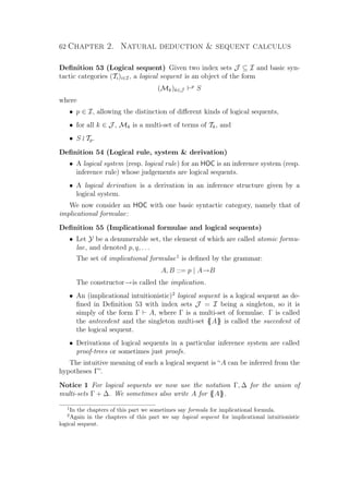
![2.1. Logical systems intuitionistic logic 63
Natural deduction is a logical system introduced by Gentzen [Gen35]. Its
implicational fragment in intuitionistic logic, called NJi, is given in Fig. 2.1.
ax
Γ, A A
Γ, A B
→right
Γ A→B
Γ A→B Γ A
→elim
Γ B
Figure 2.1: Logical NJi
Of the sequent calculus LJ for intuitionistic logic, also introduced by
Gentzen [Gen35], we present two versions (here for implication only): systems G1ii
and G3ii (with i for intuitionistic and i for implicational), which are respectively
presented in Fig. 2.2 and Fig. 2.3.
axm
A A
Γ A ∆, A B
cutm
Γ, ∆ B
Γ, A B
→right
Γ A→B
Γ A ∆, B C
→leftm
Γ, ∆, A→B C
Γ B
weak
Γ, A B
Γ, A, A B
cont
Γ, A B
Figure 2.2: Logical G1ii
ax
Γ, A A
Γ A Γ, A B
cut
Γ B
Γ, A B
→right
Γ A→B
Γ, A→B A Γ, A→B, B C
→left
Γ, A→B C
Figure 2.3: Logical G3ii
Definition 56 (Derivability in NJi, G1ii, G3ii) We write Γ NJ A if Γ A is
derivable in NJi, Γ G1ii A if it is derivable in G1ii (Γ G1iicf A if it is derivable
without the cutm-rule), and Γ G3ii A if it is derivable in G3ii (Γ G3iicf A if it is
derivable without the cut-rule).](https://image.slidesharecdn.com/frenchenglish-150412084606-conversion-gate01/85/French-english-87-320.jpg)
![2.1. Logical systems intuitionistic logic 65
the conclusion is shared between all the premisses, being duplicated in rules with
at least two premisses, and being erased in rules with no premisses such as the
axiom. For rules with exactly one premiss, the notions of context-splitting and
context-sharing is the same.
Sometimes, context-splitting rules are said to be multiplicative (hence the
subscript m in the name of the rules), while context-sharing rules are said to be
additive. Note that NJi is a context-sharing/additive system, like G3ii.
System G1ii and G3ii already illustrate the diversity of systems that exist in the
literature for sequent calculus (including G4ii, which we investigate in Chapter 7),
with quite a bewildering nomenclature.
Our G1ii-system here matches the implicational fragment of both the G1i-
system of [TS00] and the G0i-system of [NvP01]. These slightly differ from earlier
work by Kleene [Kle52] whose intuitionistic G1-system sticks to Gentzen’s original
presentation of LJ where the antecedent is a list of formulae instead of a multi-set,
with an inference rule called exchange:
Γ, A, B, ∆ C
Γ, B, A, ∆ C
The terminology G1, G2, G3 originates from the sequent calculi presented
in [Kle52], which differ from each other in the way they treat structural rules, i.e.
weakening, contraction and exchange. G1-systems make them explicit as rules,
whilst G3-systems incorporate them into the other rules.
Our system G3ii is exactly the implicational fragment Kleene’s intuitionistic
G3, from which both [TS00] and [NvP01] differ (ax is restricted to A being an
atomic formula, and the antecedent formula A→B is systematically dropped in
the second premiss of → left, building on Kleene’s variant G3a where arbitrary
omissions of formulae are allowed in the premisses of the rules).
Remark 50 In G3-systems such as G3ii, weakenings are hidden in the ax-rule
and contractions are hidden in the context-sharing rules and in the fact that
principal formulae of the antecedent are already in the premisses.
The following lemma holds:
Lemma 51 Weakening and contraction are height-preserving admissible in G3ii
and in NJi.
Proof: Straightforward induction on derivations. P
This is used to establish the following equivalence:
Theorem 52 (Logical equivalence of G1ii, G3ii NJi)
Γ G1ii A if and only if Γ G3ii A if and only if Γ NJ A.](https://image.slidesharecdn.com/frenchenglish-150412084606-conversion-gate01/85/French-english-89-320.jpg)
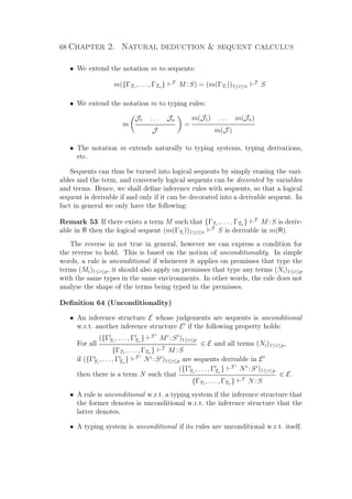
![2.2. Typing systems 69
Now we can prove:
Remark 54 There exists a term M such that {ΓT1 , . . . , ΓTn } T
M :A is deriv-
able in an unconditional typing system R if and only if the logical sequent
(m(ΓTi
))1≤i≤n
T
A is derivable in m(R).
Typing systems are often unconditional when the typed terms reflect precisely
the structure of their typing derivations, and thus that of the logical derivations
obtained by erasing the variable and term annotations.
This is the basis of the Curry-Howard paradigm, according to which the
terms/types/reduction of a typed HOC respectively correspond to the
proofs/propositions/proof transformations of a logical system. Such a correspon-
dence gives a double reading of proofs as programs and programs as proofs, so
that insight into one aspect helps the understanding of the other. A good account
can be found in e.g. [SU06].
In unconditional systems, such as those used in the Curry-Howard paradigm,
we can define a notion that corresponds to the notion of admissibility in the
logical system obtained by erasing the variable and term annotations:
Definition 65 (Term-irrelevant admissibility)
Suppose R is an unconditional typing system. A rule
J1 . . . Jp
· · · · · · · · · · · · · · · · · · · · · · ··
{ΓT1 , . . . , ΓTn } T
M :S
6
that is unconditional w.r.t. R is term-irrelevantly admissible in R if the following
property holds:
If the premisses J1, . . . , Jp are derivable in R,
then there exists a derivation in R of {ΓT1 , . . . , ΓTn } T
M :S for some term M .
Remark 55 The notion of term-irrelevant admissibility corresponds to the stan-
dard notion of admissibility (Definition 11) when term annotations are erased:
J1 . . . Jn
· · · · · · · · · · · · ··
J
is term-irrelevantly admissible in an unconditional typing system
R,
if and only if
m
J1 . . . Jn
· · · · · · · · · · · · ··
J
is admissible in m(R).
We now give a canonical way to generate typing systems for the Curry-Howard
paradigm, with one term construct for each derivation step. These typing systems
are called canonical typing systems, and we give here the definition for only a
particular kind of HOC:
6
Note the use of the dotted line to indicate this notion of admissibility as well.](https://image.slidesharecdn.com/frenchenglish-150412084606-conversion-gate01/85/French-english-93-320.jpg)
![72 Chapter 2. Natural deduction sequent calculus
• the rules with several premisses are environment-splitting.
Most chapters of this dissertation investigate additive typing systems, but an
example of multiplicative system is the object of Chapter 5. Some other typing
systems are mixtures of multiplicative and additive systems (e.g. in Chapter 7).
In the additive case, the constraint of being well-formed becomes empty: no
restriction on terms is suggested by the typing system. In the multiplicative
case, the constraint can be strengthened as the notion of linearity on terms,
which, indeed, can be considered before and independently from the notion of
typing:
Definition 69 (Linearity) A term M is linear if
• in every sub-term x.N we have x ∈ FV(N), and
• in every sub-term c(N1, . . . , Nn) the sets (FV(Ni))1≤i≤n are pairwise disjoint.
Remark 56 Indeed, if {ΓT1 , . . . , ΓTn } T
M : A is derivable in a multiplicative
system, then M is linear.
From now on, throughout the chapters of Part I and unless otherwise stated,
types are the implicational formulae7
of Definition 55. Atomic types are atomic
formulae (a.k.a. type variables), still denoted p, q, . . . The intuitive meaning of the
decorated sequent Γ M :A is that each use of a free variable in M corresponds
to the “logical use of an hypothesis of Γ to derive A”.
In the next section we start with the traditional Curry-Howard correspondence
between NJi and the simply-typed λ-calculus [Chu41] as described in [How80],
and then we introduce an HOC for a similar correspondence for G3ii.
2.3 Natural deduction λ-calculus
Definition 70 (Syntax of λ-calculus) The syntax of λ-calculus [Chu41] is de-
fined as follows:
M, N ::= x | λx.M | M N
where x ranges over a denumerable set of variables.
Terms of the form λx.M are called a (λ)-abstractions, and those of the form
M N applications.
Definition 71 (β-reduction η-reduction) The notion of reduction is β-
reduction and η-reduction defined by the following rules:
β (λx.M) N −→ N
x M
η λx.M x −→ M if x ∈ FV(M)
7
Hence, by principal type we mean principal formula rather than the principal type of a term
in implicitly or explicitly polymorphic systems and intersection type systems.](https://image.slidesharecdn.com/frenchenglish-150412084606-conversion-gate01/85/French-english-96-320.jpg)
![2.3. Natural deduction λ-calculus 73
We say that a λ-term is normal if it is a β-normal form.
We now present a typing system for λ-calculus, called the simply-typed λ-
calculus8
[GTL89].
Definition 72 (Simply-typed λ-calculus) We write Γ λ M :A if the sequent
Γ M :A is derivable with the inference rules of Fig. 2.4.
ax
Γ, x:A x:A
Γ, x:A M :B
→right
Γ λx.M :A→B
Γ M :A→B Γ N :A
→elim
Γ M N :B
Figure 2.4: Typing rules for λ-calculus
Note how the typing rules match those of Fig. 2.1, in that the erasure of
variable and term annotations (of Definition 63) of the typing system is exactly
the logical system.
Remark 57 By Remark 54, Γ NJ A if and only if Γ and M can be found such
that Γ λ M :A with Γ = m(Γ ).
This is the basis of the Curry-Howard correspondence [How80].
Definition 73 (Value) Those terms of the form x or λx.M are called val-
ues and are ranged over by V, V , . . . These are the term constructs typed by
(right-)introduction rules.
Remark 58 The fact that weakening and contraction are admissible in NJi
(Lemma 51) can be seen with terms:
Γ M :B
· · · · · · · · · · · · · · ··
Γ, x:A M :B
and
Γ, x:A, y:A M :B
· · · · · · · · · · · · · · · · · · · ·
Γ, x:A M :B
are term-irrelevantly admissible rules in the simply-typed system of λ-calculus.
The fact that they are even height-preserving admissible can be seen if in each
case we give the term M that works:
Γ M :B
− − − − − − −
Γ, x:A M :B
and
Γ, x:A, y:A M :B
− − − − − − − − −
Γ, x:A {x
y}M :B
are height-preserving rules in the simply-typed system of λ-calculus.
8
The adjective “simply” opposes this typing system to more complicated ones, as we shall
see e.g. in Chapter 4.](https://image.slidesharecdn.com/frenchenglish-150412084606-conversion-gate01/85/French-english-97-320.jpg)
![74 Chapter 2. Natural deduction sequent calculus
Remark 59 The notion of being free in a proof-term expresses whether an an-
tecedent type of the sequent is actually used in the proof. Indeed, the following
rule is also height-preserving admissible:
Γ, x:A M :B x ∈ FV(M)
− − − − − − − − − − − − −
Γ M :B
Finally, we give three main theorems of the λ-calculus that we use later:
Theorem 60 (Confluence of λ-calculus) −→β and −→β,η are confluent.
Proof: See e.g. [Bar84]. P
Theorem 61 (Typing of substitution) The following rule is admissible9
in
the simply-typed system of λ-calculus:
Γ λ N :A Γ, x:A λ M :B
· · · · · · · · · · · · · · · · · · · · · · · · · · · · · · ·
Γ λ
N
x M :B
Proof: See e.g. [GTL89]. P
Theorem 62 (Strong Normalisation of the simply-typed λ-calculus)
If Γ λ M :A then M ∈ SNβη
.
Proof: See e.g. [GTL89]. P
2.4 An HOC for G3ii
Formalisms where structural rules are treated implicitly, such as LJ or G3ii, can
be turned into typing systems of HOC without implying any condition on sub-
terms and free variables such as linearity or similar notions. Just as the purely
logical system NJi is a typing system of λ-calculus, G3ii can also be turned into the
typing system of an HOC, which we call λG3. This syntax can be found in various
textbooks (e.g. [TS00]) and papers (e.g. [DP99b]) with notational variants. It is
defined as follows:
Definition 74 (λG3)
M, N, P ::= x | λx.M | x[M, y.N] | M † x.N
where x ranges over a denumerable set of variables (which form a syntactic cat-
egory of their own).
The last constructor of the syntax is called the cut-constructor, and we call
λG3cf
the sub-syntax made without it.
9
Note that in general it is not height-preserving admissible.](https://image.slidesharecdn.com/frenchenglish-150412084606-conversion-gate01/85/French-english-98-320.jpg)
![2.4. An HOC for G3ii 75
Definition 75 (Simply-typed λG3-calculus) We write Γ λG3 M : A if the
sequent is derivable with the inference rules of Fig. 2.5, and Γ λG3cf M :A if it is
derivable without the cut-rule (i.e. M ∈ λG3cf
).
ax
Γ, x:A x:A
Γ M :A Γ, x:A N :B
cut
Γ M † x.N :B
Γ, x:A M :B
→right
Γ λx.M :A→B
Γ, x:A→B M :A Γ, x:A→B, y:B N :C
→left
Γ, x:A→B x[M, y.N]:C
Figure 2.5: G3ii
Note how the typing rules match those of Fig. 2.3, in that the erasure of
variable and term annotations (of Definition 63) of the typing system is exactly
the logical system.
Remark 63 By Remark 54, Γ G3ii A (resp. Γ G3iicf A) if and only if Γ and M
can be found such that Γ λG3 M :A (resp. Γ λG3cf M :A) with Γ = m(Γ ).
Definition 76 (Value covalue)
• Those terms of the form x or λx.M are called values and are ranged over
by V, V , . . .
• We say that M is an x-covalue if M = x or M = x[N, y.P] for some N, y, P
with x ∈ FV (N) ∪ FV (P).
At this point we can already notice that values are constructs typed by a deriv-
able sequent whose succedent is (logically) principal. Similarly, typed y-covalues
correspond to those proofs of a sequent in the last step of which the type of y is
logically principal.
It is clear that the λ-abstraction is the same as in the λ-calculus, and it will
be made clear that the cut-constructor is very similar to a let. . . in construct or
an explicit substitution.
Remark 64 As in Remark 58, the fact that weakening and contraction are
height-preserving admissible in LJ (Lemma 51) can be seen with terms:
Γ M :B
− − − − − − −
Γ, x:A M :B
and
Γ, x:A, y:A M :B
− − − − − − − − −
Γ, x:A {x
y}M :B
are height-preserving admissible rules.](https://image.slidesharecdn.com/frenchenglish-150412084606-conversion-gate01/85/French-english-99-320.jpg)
![76 Chapter 2. Natural deduction sequent calculus
Remark 65 Again, the notion of being free in a proof-term expresses whether
an antecedent type of the sequent is actually used in the proof. Indeed, the
following rule is also admissible:
Γ, x:A M :B x ∈ FV(M)
− − − − − − − − − − − − −
Γ M :B
Note that various HOC, similar to these proof-terms for G3ii, can be introduced
for classical sequent calculus, see e.g. [CH00, Urb00, Len03].
2.5 Encodings to from λ-calculus
In order to understand the semantics of such a term syntax for G3ii, we can re-
express Gentzen’s translation of proofs in sequent calculus to natural deductions
using λG3-terms and λ-terms.
G1
(x) := x
G1
(λx.M) := λx.G1
(M)
G1
(x[M, y.N]) := x G1(M)
y G1
(N)
G1
( M † x.N ) := G1(M)
x G1
(N)
Notice that terms of λG3cf
are always mapped to λ-terms in normal form.
We can also a give backward translation from natural deduction to sequent
calculus:
G2
(x) := x
G2
(λx.M) := λx.G2
(M)
G2
(M N) := G2
(M) † x.x[G2
(N), y.y]
Interestingly enough, normal forms of λ-calculus are not necessarily mapped to
λG3cf
-terms. This is fixed by Prawitz’s encoding [Pra65]:
Pr(x) := x
Pr(λx.M) := λx.Pr(M)
Pr(M N) := Prx.x(M N)
Prx.Q(y M) := y[Pr(M), x.Q]
Prx.Q((λy.N) M) := λy.Pr(N) † z.z[Pr(M), x.Q]
Prx.Q(N1 N2 M) := Prz.z[Pr(M),x.Q](N1 N2)
requiring n ≥ 1 in the last two lines.](https://image.slidesharecdn.com/frenchenglish-150412084606-conversion-gate01/85/French-english-100-320.jpg)
![Conclusion 77
Theorem 66 (Preservation of typing)
• If Γ λG3 M :A then Γ λ G1
(M):A.
• If Γ λ M :A then Γ λG3 G2
(M):A.
• If Γ λ M N :A and Γ, x:A λG3 Pr(M):B then Γ λG3 Prx.Q(M N):B.
• If Γ λ M :A then Γ λG3 Pr(M):A.
Proof: Straightforward induction on derivations, using Theorem 61. P
The following theorems can be found in the literature, some of them
in [DP99b].
Theorem 67 (Properties of the encodings)
• G1
is surjective, G1
|λG3cf is surjective on normal λ-terms, and neither is
injective.
• G2
and Pr are both injective but not surjective on λG3.
• G1
◦ G2
= Idλ and G1
◦ Pr = Idλ
• Neither G2
◦ G1
= IdλG3 nor Pr ◦ G1
= IdλG3.
• G2
◦ G1
does not leave λG3cf
stable but Pr ◦ G1
does.
Proof: Straightforward induction on terms. P
Conclusion
The first part of this chapter gives some directions for further work. The first
is a generalisation to every logical systems of the notions of additive and mul-
tiplicative rules, introduction and elimination rules, principal formula, logically
principal formula, context, etc. The second is a generic mechanism that would
produce a canonical typing system that corresponds, when variable and term an-
notations are erased, to a given logical system, so that they form a Curry-Howard
correspondence.](https://image.slidesharecdn.com/frenchenglish-150412084606-conversion-gate01/85/French-english-101-320.jpg)

![Chapter 3
Call-by-value λ-calculus
This chapter presents a few new results about λ-calculus.
The call-by-name (CBN) and call-by-value (CBV ) disciplines occur both as
particular reduction strategies in functional programming (leaving no choice as
for which redex is to be reduced), and also more simply (in various λ-calculi) as
two sub-calculi that can be interpreted with particular denotational semantics.
Theorems relating the two aspects can be found in [Plo75], and here we are
interested in the second, i.e. with no particular constraint about the context in
which we perform root reductions.
While the CBN λ-calculus is simply the full λ-calculus, with β-reduction and
possibly η-reduction (as presented in Chapter 2), the notion of CBV λ-calculus
seems less canonical:
In [Plo75], a calculus called λV is introduced, whose terms are exactly those
of λ-calculus and whose reduction rule βV is merely β-reduction restricted to the
case where the argument is a value V , i.e. a variable or an abstraction.
βV (λx.M) V −→ V
x M
Clearly, in the fragment λEvalArg of λ-calculus where all arguments are values,
βV = β. Hence, applying CBN- (general β) or CBV- (βV) reduction is the same,
a property that is called strategy indifference.
Using the notion of continuation, of which a history can be found in [Rey93],
the (CBN) λ-calculus can be encoded into λEvalArg with a continuation-passing-
style (CPS) translation in a way such that two terms are β-equivalent if and only
if their encodings are β/βV-equivalent [Plo75]. Similarly, two CPS-translations
into λEvalArg can be defined for the CBV calculus λV: Reynolds’ [Rey72, Rey98]
and Fischer’s [Fis72, Fis93], which only differ in the order of two arguments
appearing in these translations. Both of them are sound, in that in each case
two βV-equivalent λ-terms are mapped to two β/βV-equivalent terms, but they
are incomplete in that the β/βV-equivalence in λEvalArg is bigger than needed (see
e.g. [Plo75]).
79](https://image.slidesharecdn.com/frenchenglish-150412084606-conversion-gate01/85/French-english-103-320.jpg)
![80 Chapter 3. Call-by-value λ-calculus
Strongly related to the idea of monad and monadic λ-calculus [Mog91], Moggi’s
λC-calculus [Mog88] extends λV with a let _ = _ in _ constructor and new re-
duction rules, such as:
letV let x = V in M −→ V
x M
In particular, with the use of this constructor, an application cannot be a normal
form if one of its sides is not a value.
Both aforementioned CPS-translations can be extended to λC, in a way such
that they are both sound and complete. Alternatively, the new constructor can
be avoided and represented as a β-redex, and the reduction rules can then be
expressed as manipulations (essentially, permutations) of β-redexes, with the
same properties (e.g. [SF93] for the case of Fischer).
More refined investigations about the CBV λ-calculus consist of analysing
how reduction, rather than equivalence, is preserved by CPS-translations. In
other words, the question arises of how CPS-translations could be made not only
equational correspondences, but also Galois connections or reflections (see Defi-
nition 7). The two aforementioned translations, in their original forms, construct
redexes that do not correspond to those redexes present in the term that they
translate. Directly reducing some of them, which are called administrative re-
dexes, produces refined versions of the Reynolds and Fischer translations.
In [SW97], a refined Reynolds translation (with a reverse translation) is proved
to form a reflection in λC of its target calculus λR
CPS. It is also stated that a
particular refined Fischer translation cannot be a reflection, nor can it even be a
Galois connection from λC. We claim here that a different choice of which redexes
are considered administrative, which seems more natural, leads to a different
refined version of the Fischer translation that does form a reflection of its target
calculus λF
CPS in (a minor variation of) λC.
We leave the discussion about administrative redexes for section 3.1. The
minor variation of λC consists of replacing rule βV with the following:
B (λx.M) N −→ let x = N in M
This change is justified for four reasons:
• This variation makes our refined Fischer translation a reflection in λC of its
target calculus.
• It is closer to a sequent calculus called LJQ and presented in Chapter 6 as
the CBV-fragment of G3ii from Chapter 2.
• It does not change the equational theory of λC.
• Splitting βV into B followed by letV seems more atomic and natural, with
only one rule controlling whether a particular sub-term is a value or not.](https://image.slidesharecdn.com/frenchenglish-150412084606-conversion-gate01/85/French-english-104-320.jpg)
![3.1. λV CPS-translations 81
From the reflection result we can also prove (Theorem 5) that our version of
λC is confluent, using the confluence of λF
CPS. The latter is a simple consequence
of the confluence of β-reduction in λ-calculus (Theorem 60) and the fact that
λF
CPS is stable under β/βV-reduction.
All these results (reflection, confluence, etc. ) also hold with (CBV) η-reduction
added, e.g. in λV with the rule:
ηV λx.V x −→ V if x ∈ FV(V )
Unfortunately, confluence of λF
CPS with its corresponding η-reduction rules ηV1
and ηV2 is not as direct as with β-reduction only, since λF
CPS is not stable under
general η-reduction1
(so we cannot directly use Theorem 60). Since we could not
find a proof of this result in the literature, we establish it as follows:
• we consider the closure λ+
CPS of λF
CPS under general β, η-reduction, which we
know to be confluent from Theorem 60,
• we establish a reflection in λ+
CPS of λF
CPS and use Theorem 5.
Section 3.1 presents Plotkin’s CBV λV-calculus [Plo75], the Reynolds and Fis-
cher continuation-passing style (CPS) translations from λV. Section 3.2 iden-
tifies the target calculi λR
CPS and λF
CPS, and proves the confluence of λF
CPS. Sec-
tion 3.3 presents Moggi’s λC-calculus [Mog88] extending λV, in which the extended
Reynolds translation and its reverse translation were proved to form a reflection
of λR
CPS [SW97]. In section 3.4 we prove that the extended Fischer translation
and its reverse translation, which we here introduce, similarly form a reflection
of λF
CPS in our slightly modified version of λC.
3.1 λV CPS-translations
Now we present the λV-calculus:
Definition 77 (λV) The syntax of λV is the same as that of λ-calculus, although
it is elegant to present it by letting values form a syntactic category of their own:
V, W, . . . ::= x | λx.M
M, N, . . . ::= V | M N
V, W, . . . stand for values, i.e. variables or abstractions.
We obtain the reduction rules of λV by restricting β-reduction to the cases
where the argument is a value and restricting η-reduction to the cases where the
function is a value:
βV (λx.M) V −→ V
x M
ηV λx.V x −→ V if x ∈ FV(V )
1
In fact, even λEvalArg is not stable under general η-reduction.](https://image.slidesharecdn.com/frenchenglish-150412084606-conversion-gate01/85/French-english-105-320.jpg)
![82 Chapter 3. Call-by-value λ-calculus
In presence of βV, the following rule has the same effect as ηV:
ηV λx.y x −→ y if x = y
Definition 78 (λEvalArg) λEvalArg is the fragment of λ-calculus where all argu-
ments are values, hence given by the following syntax:
V, W, . . . ::= x | λx.M
M, N, . . . ::= V | M V
Remark 68 (Strategy indifference) In the λEvalArg fragment, βV = β, so ap-
plying CBN- (general β) or CBV- (βV) reduction is the same.
Note that the situation is different for η-conversion in λEvalArg, since ηV = η.
The fragment λEvalArg is stable under βV/β-reduction and under ηV-reduction, but
not under η-reduction.
We can encode λV into λEvalArg by using the notion of continuation and defin-
ing Continuation Passing Style translations (CPS-translations). There are in
fact two variants of the CBV CPS-translation: Reynolds’ [Rey72, Rey98] and
Fischer’s [Fis72, Fis93], presented in Fig. 3.1.
R(V ) := λk.k RV(V )
R(M N) := λk.R(M) (λx.R(N) (λy.x y k))
RV(x) := x
RV(λx.M) := λx.λk.R(M) k
Reynolds’ translation
F(V ) := λk.k FV(V )
F(M N) := λk.F(M) (λx.F(N) (λy.x k y))
FV(x) := x
FV(λx.M) := λk.λx.F(M) k
Fischer’s translation
Figure 3.1: CBV CPS-translations
Note that the two translations only differ in the order of arguments in x y k
/ x k y and λx.λk.R(M) k / λk.λx.F(M) k.
As mentioned in the introduction, both translations map βV-equivalent terms
to β/βV-equivalent terms (soundness), but the converse fails (incompleteness)
(see e.g. [Plo75]).
A more refined analysis is given by looking at the reduction rather than just
equivalence. Note that the two translations above introduce many fresh vari-
ables, but bind them, often leading to new redexes and potential redexes not
corresponding to redexes in the original terms. Some of these get in the way of](https://image.slidesharecdn.com/frenchenglish-150412084606-conversion-gate01/85/French-english-106-320.jpg)
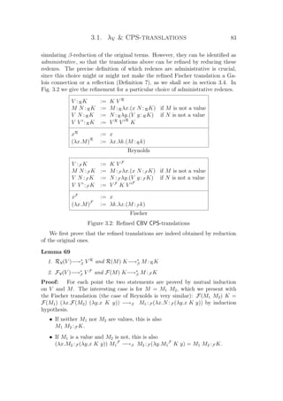
![84 Chapter 3. Call-by-value λ-calculus
• If M1 is not a value but M2 is, this is also
M1 :F (λx.(λy.x K y) M2
F
) −→β M1 :F (λx.x K M2
F
) = M1 M2 :F K.
• If both M1 and M2 are values, this is also
(λx.(λy.x K y) M2
F
) M1
F
−→∗
β M1
F
K M2
F
= M1 M2 :F K.
P
Remark 70 Note that K is a sub-term of M :RK and M :F K with exactly
one occurrence2
, so for instance if x ∈ FV(K) FV(M) then x has exactly one
free occurrence in M :RK and M :F K. Hence, the variables introduced by the
translations and denoted by k, which we call the continuation variables, are such
that the set of those that are free in the scope of a binder λk. is exactly {k}, with
exactly one occurrence (only one of them can be free at a time).
In other words, in a term (which is a α-equivalence class of syntactic terms,
i.e. a set) there is always a representative that always uses the same variable
k. Note that K does not need to range over all λ-terms for the definition of
the refined translations to make sense, but only over constructs of the form k or
λx.M, with x = k.
In that case, note that if we call continuation redex any β-redex binding a
continuation variable (i.e. of the form (λk.M) N), then the refined Reynolds
translation considers all continuation redexes administrative and has thus re-
duced all of them, while the refined Fischer translation leaves a continuation
redex in the construct (λx.M) V :F K = (λk.λx.M :F k) K V F
, which is thus not
administrative.
This choice is different from that of [SW97] which, as for the Reynolds trans-
lation, considers all continuation redexes administrative. With that choice they
establish negative results about the refined Fischer translation as we shall discuss
in section 3.4.
We can now identify the target calculi of the refined translations, i.e. the
fragments of λ-calculus reached by them, and look at their associated notions of
reduction.
3.2 The CPS calculi λR
CPS λF
CPS
From the refined Reynolds and Fischer translations we get the target fragments
of λ-calculus described in Fig. 3.3.
• M, N, . . . denote (CPS-)programs,
• V, W, . . . denote (CPS-)values,
• K, K , . . . denote continuations.](https://image.slidesharecdn.com/frenchenglish-150412084606-conversion-gate01/85/French-english-108-320.jpg)
![86 Chapter 3. Call-by-value λ-calculus
A good account of the refined Reynolds translation as a reflection can be found
in [SW97], so here we study similar properties for the refined Fischer translation,
building on earlier work [SF93] that established results of equational correspon-
dence. Moreover, Fischer’s approach helps establishing connections between CBV-
λ-calculus and a particular fragment of G3ii called LJQ and studied in Chapter 6.
We now establish the confluence of λF
CPS. The confluence of λF
CPSβ is straight-
forward, since every case of β-reduction in λF
CPS is covered by either βV1 or βV2, so
it is a particular case of the confluence of β-reduction in λ-calculus (Theorem 60).
For λF
CPSβη we use the confluence of β, η-reduction in λ-calculus, but unfortu-
nately the grammar of λF
CPS is not stable under β, η. Fig. 3.5 shows its closure
λ+
CPS under β, η.
M, N ::= K V
V, W ::= x | λk.K
K ::= k | λx.M | V K
Figure 3.5: Grammar of λ+
CPS
First, note that we no longer have β = βV. Second, this grammar is indeed
stable under β, η; all the cases are:
(λx.M) V −→β
V
x M
(λk.K) K −→β
K
k K
λk.V k −→η V
λx.K x −→η K if x ∈ FV(K)
We can then take β, η as the reductions of λ+
CPS, and derive from the confluence
of λ-calculus (Theorem 60) that β and η are confluent in λ+
CPS.
Note that λ+
CPS is the smallest grammar that includes that of λF
CPS and that
is stable under β, η: Fig. 3.6 defines a mapping ⇑ from λ+
CPS onto λF
CPS such that
⇑ M −→η M. Our convention for parentheses assumes that ⇑ applies to the
smallest expression on its right-hand side.
Remark 71 Note that ⇑ M −→η M, ⇑ V −→η V , ⇑ K −→η K and if M, V ,
K are in λF
CPS then ⇑ M = M, ⇑ V = V , ⇑ K = K.
We can now prove the following:
Theorem 72 (⇑ is a Galois connection) The identity IdλF
CPS
and the map-
ping ⇑ form a Galois connection from λF
CPS, equipped with λF
CPSβη, to λ+
CPS, equipped
with βV (and also with only λF
CPSβ and β).
Proof: Given Remark 71, it suffices to check the simulations:
• For the simulation of η by λF
CPSβη through ⇑, we check all cases:](https://image.slidesharecdn.com/frenchenglish-150412084606-conversion-gate01/85/French-english-110-320.jpg)
![3.3. Moggi’s λC-calculus 89
and with the following rules:
M N −→ let x = M in (x N) if M is not a value
V N −→ let y = N in (V y) if N is not a value
Indeed, for both refined translations, a redex of these rules and its reduced form
are mapped to the same term.
This extension is related to Moggi’s monadic λ-calculus [Mog91], which sug-
gests additional rules to form the CBV-calculus λC [Mog88]3
defined as follows:
Definition 79 (λC) The terms of λC are given by the following grammar:
V, W, . . . ::= x | λx.M
M, N, P, . . . ::= V | M N | let x = M in N
The reduction system of λC is given in Fig. 3.7.
βV (λx.M) V −→ V
x M
letV let x = V in M −→ V
x M
let1 M N −→ let x = M in (x N)
(M not a value)
let2 V N −→ let y = N in (V y)
(N not a value)
assoc let y = (let x = M in N) in P −→ let x = M in (let y = N in P)
Figure 3.7: Rules of λC
Again, η-reduction can be added:
ηlet let x = M in x −→ M
ηV λx.(V x) −→ V if x ∈ FV (V )
And again, in presence of βV , rule ηV has the same effect as the following one:
ηV λx.(y x) −→ y if x = y
For various purposes described in the introduction, here we also consider a
slight variation of λC, in which reduction is refined by replacing the reduction
rule βV with the following:
B (λx.M) N −→ let x = N in M
This allows the split of the rule βV into two steps: B followed by letV. Note that
in B we do not require N to be a value. Such a restriction will only apply when
reducing let x = N in M by rule letV.
3
A detailed presentation of these ideas can also be found in [SW97].](https://image.slidesharecdn.com/frenchenglish-150412084606-conversion-gate01/85/French-english-113-320.jpg)
![90 Chapter 3. Call-by-value λ-calculus
System λCβ is B, letV, let1, let2, assoc and λCβη is λCβ, ηlet, ηV.
In [SF93] it is shown that, in effect, Fischer’s translation forms an equational
correspondence between (Moggi’s original) λC and λF
CPS. In [SW97], Sabry and
Wadler establish not only that Reynolds’ translation form an equational cor-
respondence between (Moggi’s original) λC and λR
CPS, but the refined Reynolds
translation actually forms a reflection.
3.4 The refined Fischer translation is a reflection
In [SW97], Sabry and Wadler also establish that for a particular definition of
administrative redex (namely, every β-redex with a binder on the continuation
variable k is administrative), the refined Fischer translation cannot be a reflection,
and from from λC to λF
CPS it cannot even be a Galois connection.
Here we show that our (different) choice of administrative redex for the Fischer
translation (given in Fig. 3.2) makes it a reflection of λF
CPS in our version of λC,
where the rule βV is decomposed into two steps as described above. This will
also bring λC closer to a particular fragment of λG3 called LJQ and studied in
Chapter 6.
Lemma 74
1. K
k (M :F K) = M :F
K
k K
2. V F
x (M :F K) = V
x M :F
V F
x K and V F
x WF
= ( V
x W)
F
.
3. If K −→λF
CPSβ
K then M :F K −→λF
CPSβ
M :F K
(and similarly for −→λF
CPSβη
).
Proof: Straightforward induction on M for the first and third points and on
M and W for the second. P
Theorem 75 (Simulation of λC in λF
CPS) The reduction relation −→λCβ
(resp. −→λCβη
) is (weakly) simulated by −→λF
CPSβ
(resp. −→λF
CPSβη
) through
the refined Fischer translation.
Proof: By induction on the size of the term being reduced: We check all the
root reduction cases, relying on Lemma 74:](https://image.slidesharecdn.com/frenchenglish-150412084606-conversion-gate01/85/French-english-114-320.jpg)
![Chapter 4
Two refinements of the simulation
technique
In this chapter, whose contents appeared in [Len05], we develop two refine-
ments of the simulation technique (Corollary 26) that were originally designed
for deriving strong normalisation results from the strong normalisation of typed
λ-calculus (Theorem 62).
The first technique, presented in section 4.1 and called the Safeness Mini-
mality technique, turns out to be more general and can be applied to any HOC.
In contrast to other results, our proof of the main theorem about this technique
is only valid in classical logic.
As an example, we show how this technique can be used for the explicit sub-
stitution calculus λx [BR95], yielding a short proof of Preservation of Strong
Normalisation (PSN) [BBLRD96]. The technique also allows us to easily derive
the strong normalisation of typed terms from that of typed λ-terms. Unfortu-
nately, since the technique is fundamentally classical, it cannot draw advantage
of the constructive proofs of strong normalisation such as the one in [JM03] for
the simply-typed λ-calculus.
The second technique, presented in section 4.2, is more specifically designed
for proving normalisation results that are related to normalisation of β-reduction
in λ-calculus. It consists in simulating an HOC in the calculus λI of [Klo80],
when a simple attempt of simulation in λ-calculus fails. Its applicability holds
in intuitionistic logic, apart maybe from one external result, whose provability in
intuitionistic logic remains to be checked.
An example of how this technique can be applied is given in Chapter 5 to
prove the PSN property of an explicit substitution calculus called λlxr with full
composition of substitutions, for which standard techniques that we tried all
failed. This is a new result. Note that a presentation of λlxr has been published
by Kesner and Lengrand in [KL05, KL07].
95](https://image.slidesharecdn.com/frenchenglish-150412084606-conversion-gate01/85/French-english-119-320.jpg)
![96 Chapter 4. Refining the simulation technique
λx
λ
λlxr
λ
A CQ
Figure 4.1: Standard and generalised situations for stating PSN
Preservation of Strong Normalisation
An important normalisation property related to λ-calculus is the Preservation of
Strong Normalisation (PSN) [BBLRD96]. It concerns syntactic extensions of λ-
calculus with their own reduction relations and states that if a λ-term is strongly
normalising for β-reduction, then it is still strongly normalising when considered
as a term of the extended calculus, subject to the reductions of the latter. In
other words, the reduction relation should not be too big, although it is often
required to be big enough to simulate β-reduction.
The definition of the PSN property can be slightly generalised for calculi in
which λ-calculus can be embedded (by a one-to-one translation, say A) rather than
just included. In that case PSN states that if a λ-term is strongly normalising,
then its encoding is also strongly normalising.
Fig. 4.1 illustrates the two situations with the examples of the calculus
λx [BR95] and the calculus λlxr, introduced in Chapter 5: the former is a syntactic
extension of λ-calculus, while the latter can encode the λ-calculus.
As discussed below, λx and λlxr are calculi with explicit substitutions.
Calculi with explicit substitutions
Indeed, examples of cases where the PSN property is relevant are the calculi
with explicit substitutions. Such constructs, which use specific substitution con-
structors and which can be reduced, thus implement the notion of substitution
(Definition 43), by means of which β-reduction can usually be decomposed.
In a wider sense we can call explicit substitution a construct that can be
interpreted as (i.e. mapped to) an (implicit) substitution, with rules manipulat-
ing substitution constructors that are valid with respect to this interpretation,
and whether or not, among these manipulations, some propagation rules actu-
ally implement substitution. In that sense will constructs such as _ † _._ (of
section 2.4) or let _ = _ in _ (of section 3.3) be seen as explicit substitutions as
well.
Among the possible manipulations of explicit substitutions is the notion of
composition, in which, for instance, one explicit substitution can be permuted into
another. In the literature about explicit substitutions, which has been especially
abundant in the last 15 years (e.g. [ACCL91, BBLRD96, BR95, BBLRD96]),
an unexpected result was given by Melliès [Mel95] who gave a counter-example](https://image.slidesharecdn.com/frenchenglish-150412084606-conversion-gate01/85/French-english-120-320.jpg)
![Introduction 97
to the PSN property that applies to many calculi with explicit substitutions
with a (rather weak, but present) notion of composition, such as for example
λσ [ACCL91] or λσ⇑ [HL89].
This phenomenon shows a flaw in the design of these calculi with explicit
substitutions in that they are supposed to implement their underlying calculus
without losing its good properties such as strong normalisation of simply-typed
terms, as Melliès’ counter-example implies. PSN is in some sense a test property
when a calculus with explicit substitutions is introduced.
However, there are many ways to avoid Melliès’ counter-example in order
to recover the PSN property. One of them is simply to forbid the substitution
constructors to cross λ-abstractions [LM99, For02]; another imposes a simple
strategy on the calculus with explicit substitutions to mimic exactly the calculus
without explicit substitutions [GL98]; another simply consists of avoiding com-
position of substitutions [BBLRD96]. The first solution leads to weak λ-calculi,
not able to express strong β-equality, which is used for example in implementa-
tions of proof-assistants [Coq, HOL]. The second solution exploits very little of
the notion of explicit substitutions because they can be neither composed nor
even delayed. The last one is simple but composition of substitutions is useful
in implementations of higher-order unification [DHK95, DHKP96] or functional
abstract machines [HMP96].
The solution [BBLRD96] for the calculus with explicit substitutions λx [BR95],
whose syntax extends that of λ-calculus, is investigated in section 4.1.1, with a
proof of PSN. Its explicit substitutions are of the form M/x N, in which the
variable x is bound in N and the sub-term M is called the body. Most explicit
substitutions in this dissertation (except from section 9.5 which uses de Bruijn
indices [dB72]) are of this form as well. Of course, the techniques of this chapter
are likely to be adaptable to other frameworks, e.g. with de Bruijn indices [dB72]
or additional parameters.
Another example of calculus with explicit substitutions is λlxr, introduced in
Chapter 5 and also presented in [KL05, KL07]. It uses the same form of explicit
substitutions as above but requires terms to be linear and hence is not a syntactic
extension of λ-calculus. However the latter can be embedded in the former so
the generalised notion of PSN makes sense.
Strong normalisation of typed terms sequent calculus
Apart from PSN, other normalisation results are desirable in calculi with explicit
substitutions, such as strong normalisation of typed terms, which can sometimes
be inferred from PSN.
Among the calculi with explicit substitutions for which this is extremely rel-
evant are the intuitionistic sequent calculi [Gen35] (with term annotations), e.g.
G3ii from Chapter 2. Indeed, the most natural typing rule for an explicit sub-
stitution as expressed above is precisely a cut-rule. The notion of computation](https://image.slidesharecdn.com/frenchenglish-150412084606-conversion-gate01/85/French-english-121-320.jpg)
![98 Chapter 4. Refining the simulation technique
in sequent calculi is cut-elimination: the proof of a sequent may be simplified by
eliminating the applications of the cut-rule, so that a sequent which is provable
with the cut-rule is provable without. Many techniques aimed at proving normal-
isation results about calculi with explicit substitutions are in fact relevant for cut-
elimination in sequent calculus. In other words, termination of cut-elimination
processes can often be derived from termination of calculi with explicit substi-
tutions. Of course, in the case of sequent calculi, termination of cut-elimination
relies only on the strong normalisation of typed terms.
Failure of the simple simulation technique
The basic idea in proving that a term M of a calculus with explicit substitutions
is SN is to use Corollary 26, that is, simulating the reduction steps from M by
β-reduction steps from a strongly normalising λ-term H(M).
For PSN, if M = A(t) where t is the λ-term known to be SNβ
by hypothesis,
then we would take H(M) = t.
For sequent calculus, it would be a typed (and hence strongly normalising)
λ-term that denotes a proof in natural deduction of the same sequent (using
the Curry-Howard correspondence). The idea of simulating cut-elimination by
β-reductions has been investigated in [Zuc74].
There is one problem in doing so: an encoding into λ-calculus that allows the
simulation needs to interpret explicit substitutions by implicit substitutions such
as {u
x}t. But should x not be free in t, all reduction steps taking place within
the term of which u is the encoding would not induce any β-reduction in {u
x}t.
Therefore, the reduction relation that is only weakly simulated, i.e. the one
consisting of all the reductions that are not necessarily simulated by at least one
β-reduction, is too big to be proved terminating (and very often it is not).
The two techniques developed hereafter are designed to overcome this prob-
lem, in a somewhat general setting. The two aforementioned calculi with explicit
substitutions λx and λlxr respectively illustrate how each can be applied and can
provide in particular a proof of the PSN property. The example of λx is presented
just after the first technique, while λlxr is the object of Chapter 5.
4.1 The safeness minimality technique
Given a rewrite system R on a set of terms A, the safeness and minimality tech-
nique presents two subsystems minR and safeR satisfying
−→safeR ⊆−→minR ⊆−→R and SNminR
= SNR
.
The intuitive idea is that a reduction step is minimal if all the (strict) sub-
terms of the redex are in SNR
. Theorem 83 says that in order to prove that −→R
is terminating, we can restrict our attention to minimal reductions only, without
loss of generality.](https://image.slidesharecdn.com/frenchenglish-150412084606-conversion-gate01/85/French-english-122-320.jpg)
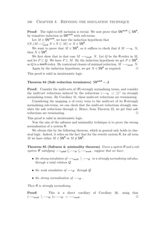
![4.1. The safeness minimality technique 101
B (λx.M) N −→ N/x M
x :
Abs N/x λy.M −→ λy. N/x M
App N/x M1 M2 −→ N/x M1 N/x M2
VarK N/x y −→ y
VarI N/x x −→ N
Figure 4.2: Reduction rules for λx
Now notice the particular case of the technique when we take R = safeR. By
Theorem 84 we would directly have its strong normalisation. Unfortunately, this
situation is often too coarse, that is to say, the relation −→R is too small, so
that −→minR −→R is often too big to be strongly simulated.
Hence, in order to define R , we use the safeness criterion, but the precise
definition depends on the calculus that is being treated. In the following section
we give the example of the λx-calculus [BR95] and prove a few normalisation
results. The technique will also be used in Chapter 6 to prove similar results
about the calculus λ [Her95], the proof being shorter than the existing ones
in [DU03] and [Kik04a].
This technique seems close to the notion of dependency pairs (see e.g. [AG00]).
Formal connections with it should be studied and is left as further work.
4.1.1 A case study: PSN of λx
Definition 82 (Syntax of λx) λx [BR95] is the syntactic extension of λ-calculus
with the aforementioned explicit substitutions:
M, N ::= x| λx.M| M N| N/x M
Definition 83 (Reduction in λx) The reduction relation of λx reduces β-redexes
into explicit substitutions which are thence evaluated, as shown in Fig. 4.2.
Note that for this system to be an atomic one (and hence be expressible as an
HRS), there should be no obvious free variable in the rules (Definitions 46 and 45).
Hence, variables should form a syntactic category of their own: in that case, rule
VarK can be read with y standing for a meta-variable of that variable category
(otherwise it could stand for a term and then we have the rule of garbage collection
N/x M −→ M). If variables form a syntactic category of their own, then the
only notion of substitution that is provided by Definition 43 is the substitution of
a variable for another variable and nothing else, but now we have a substitution
constructor to deal with other substitutions explicitly. Alternatively, one could
simply not require the system to be atomic, but then we lose the possibility to
express it as a HRS and the advantages thereof.
In this example we take R = safeB, minx.](https://image.slidesharecdn.com/frenchenglish-150412084606-conversion-gate01/85/French-english-125-320.jpg)
![104 Chapter 4. Refining the simulation technique
Γ, x : A x:A
Γ P :A Γ, (x : A) M :C
Γ P/x M :C
Γ, (x : A) M :B
Γ λx.M :A→B
Γ M :A→B Γ N :A
Γ M N :B
Figure 4.3: Typing rules for λx
In [Bon01, DL03], it is proved that typed terms are strongly normalising
by a reducibility technique. We show here that one application of the Safeness
and Minimality technique, apart from PSN, is to derive this result from the
strong normalisation of λ-calculus (Theorem 62). Indeed, it turns out that the
aforementioned encoding preserves typing:
Theorem 90 (Preservation of simple typing)
If Γ λx M :A then Γ λ H(M):A.
Proof: Straightforward induction on the typing tree. P
Corollary 91 (Strong normalisation of the simply-typed λx)
If Γ λx M :A then M ∈ SNB,x
.
Proof: By combining Theorem 62, Theorem 90 and Corollary 88. P
Moreover, this technique is quite modular, since it only relies on the preser-
vation of typing by the translation H. Hence, any typing system on λx entails
strong normalisation if typed terms are mapped by H to strongly normalising
λ-terms (maybe because these can be typed in a corresponding typing system
on λ-calculus that entails strong normalisation). We illustrate this by presenting
systems with intersection types [CD78].
Definition 84 (Types with intersections) For the purpose of this section
only, we extend the syntax of types (which, until now, were just implicational
formulae —Definition 55). The set of types with intersections is defined by the
grammar:
A, B ::= p | A→B | A ∩ B
The constructor ∩ is called the intersection.
Γ M :A Γ M :B
Γ M :A ∩ B
Γ M :A1 ∩ A2
i ∈ {1, 2}
Γ M :Ai
Figure 4.4: Intersection types for λ-calculus](https://image.slidesharecdn.com/frenchenglish-150412084606-conversion-gate01/85/French-english-128-320.jpg)
![4.1. The safeness minimality technique 105
Then we can add the two typing rules of Fig. 4.4 to those of the simply-typed
λ-calculus (presented in Fig. 2.4).
Remark 92 Note that the left-hand side rule of Fig. 4.4 is not unconditional
w.r.t. the general system, since the two premisses require the same term M.
This has long prevented the understanding of intersection types via the Curry-
Howard paradigm. Investigations into some logical counterpart to intersection
types can be found in [PRDRR05].
We write Γ λ∩ M :A when the sequent is derivable in the typing system thus
obtained, which was introduced in [CD78] and characterises SNβ
:
Theorem 93 (Strong Normalisation of λ-calculus with intersections)
Γ λ∩ M :A if and only if M ∈ SNβ
.
Proof: See e.g. [Pot80]. P
Similarly, when the three inference rules of Fig. 4.5 are added to those of
Fig. 4.3, we obtain a typing system whose derivable sequents we denote like
Γ λx∩ M :A.
Γ M :A Γ M :B
Γ M :A ∩ B
Γ M :A1 ∩ A2
i ∈ {1, 2}
Γ M :Ai
Γ M :A ∆ N :B x ∈ Dom(Γ)
Γ N/x M :A
Figure 4.5: Intersection types for λx
This typing system echoes that of intersection types for λ-calculus, since it
has the interesting property of characterising SNB,x
[LLD+
04]:
Theorem 94 (Capturing strongly normalising terms)
If M ∈ SNB,x
then there exist Γ and A such that Γ λx∩ M :A.
In [LLD+
04], the converse (typed terms are strongly normalising) is also proved
by a reducibility technique. Again we show that the Safeness and Minimality tech-
nique applies here to derive this result from the strong normalisation of λ-calculus
with intersection types (Theorem 93). Indeed, the aforementioned encoding also
preserves typing with intersections:
Theorem 95 (Preservation of typing with intersections)
If Γ λx∩ M :A then Γ λ∩ H(M):A.
Proof: Straightforward induction on the typing tree. P](https://image.slidesharecdn.com/frenchenglish-150412084606-conversion-gate01/85/French-english-129-320.jpg)
![106 Chapter 4. Refining the simulation technique
Hence, we also get:
Corollary 96 (Strong normalisation of λx typed with intersections)
If Γ λx∩ M :A then M ∈ SNB,x
.
Proof: By combining Theorem 93, Theorem 95 and Corollary 88. P
Often, this kind of strong normalisation result is derived from the PSN prop-
erty by lifting the explicit substitutions into β-redexes [Her95], but this is pre-
cisely what the encoding does in the necessary places, so that Corollary 88 is a
shortcut of Herbelin’s technique.
4.2 The simulation technique using a memory op-
erator
In this section we present another refinement of the simulation technique to prove
normalisation results of a calculus, henceforth called the calculus, that is related
to λ-calculus, for instance a calculus with explicit substitutions. In case a simple
simulation in λ-calculus fails, as described in the introduction, we suggest to use
instead the λI-calculus of [Klo80], based on earlier work by [Chu41, Ned73]. We
refer the reader to [Sør97, Xi97] for a survey on different techniques based on the
λI-calculus to infer normalisation properties.
On the one hand, λI extends the syntax of λ-calculus with a “memory opera-
tor” so that, instead of being thrown away, a term N can be retained and carried
along in a construct [ − , N]. With this operator, those bodies of substitutions
are encoded that would otherwise disappear, as described in the introduction.
On the other hand, λI restricts λ-abstractions to variables that have at least one
free occurrence, so that β-reduction never erases its argument.
Performing a simulation in λI requires the encoding to be non-deterministic,
i.e. we define a relation H between the calculus and λI, and the reason for this
is that, since the reductions in λI are non-erasing reductions, we need to add this
memory operator at random places in the encoding, using such a rule:
M H T
U ∈ ΛI
M H [T, U]
where ΛI is the set of λI-terms.
For instance, if the calculus is λ-calculus itself, we would have λx.x H λx.[x, x]
but also λx.x H [λx.x, λz.z], so that both λx.[x, x] and [λx.x, λz.z] (and also
λx.x) are encodings of λx.x.
The reduction relation of the calculus must then satisfy the hypotheses of
Corollary 26. Namely, it should be the union of a reduction relation −→Y that
is strongly simulated by −→β,π through H and a terminating reduction relation
−→Z that is weakly simulated by −→β,π through H . We then need the fact](https://image.slidesharecdn.com/frenchenglish-150412084606-conversion-gate01/85/French-english-130-320.jpg)
![4.2. Simulation with a memory operator 107
that every term M of the calculus can be encoded into a strongly normalising
term of λI, to start off the simulations. This depends on the calculus, but the
following method generally works:
1. Encode the term M as a strongly normalising λ-term t, such that no sub-
term is lost, i.e. not using implicit substitutions. For PSN, the original
λ-term would do, because it is strongly normalising by hypothesis; for a
proof-term of sequent calculus, t would be a λ-term typed in an appropriate
typing system, the typing tree of which is derived from the proof-tree of the
sequent (we would get t ∈ SNβ
using a theorem stating that typed terms
are SNβ
).
2. Using a translation i from λ-calculus to λI, introduced in this section, prove
that i(t) reduces to one of the non-deterministic encodings of M in λI, that
is, that there is a term T such that M H T and i(t)−→∗
β,π T.
In this section we prove that if a λ-term t is strongly normalising for β-reductions,
then i(t) is weakly normalising in λI. The proof simply consists of simulating
an adequate reduction sequence that starts from t and ends with a normal form,
the encoding of which is a normal form of λI. What makes this simulation work
is the fact that the reduction sequence is provided by a perpetual strategy, i.e.
a strategy that terminates on a term only if it is strongly normalising. Also,
weak normalisation implies strong normalisation in λI [Ned73], so i(t) is strongly
normalising, as well as the above λI-term T.
The technique is summarised in Fig. 4.6.
As we shall see, this technique works for proving PSN of the explicit sub-
stitution calculus λlxr of chapter 5. Furthermore, it can be combined with the
safeness and minimality technique which provides proofs of strong normalisation
for various sequent calculi, and it is, we believe, likely to be applicable to many
other calculi.
4.2.1 The λI-calculus
Definition 85 (Grammar of λI) The set ΛI of terms of the λI-calculus
of [Klo80] is defined by the following grammar:
T, U ::= x | λx.T | T U | [T, U]
with the additional restriction that every abstraction λx.T satisfies x ∈ FV(T).
We denote lists of λI-terms using vectors, and if
−→
T = T1, . . . , Tn, then U
−→
T
denotes U T1 . . . Tn and [U,
−→
T ] denotes [. . . [U, T1], . . . , Tn], assuming that these
expressions denote U when n = 0.
The following property is straightforward by induction on terms.](https://image.slidesharecdn.com/frenchenglish-150412084606-conversion-gate01/85/French-english-131-320.jpg)
![108 Chapter 4. Refining the simulation technique
the calculus λ λI
t ∈ SNβ
i()
CQ i(t)
β,π∗
M
Y Z∗
H CQ
HV
T
β,π∗
N1
Y Z∗
H CQ U1
β,π∗
Ni
Z∗
H CQ Ui
Ni+j
Z∗
H
HViiiiiiiiiiiiiiiiiiiiiiii
iiiiiiiiiiiiiiiiiiiiiiii H
R`ppppppppppppppppppppppppppppp
ppppppppppppppppppppppppppppp
Figure 4.6: The general technique to prove that M ∈ SN
Lemma 97 (Stability under substitution [Klo80])
If T, U ∈ ΛI, then U
x T ∈ ΛI.
Proof: By induction on T. P
Definition 86 (Reduction system of λI) The reduction rules are:
(β) (λx.T) U → U
x T
(π) [T, U] T → [T T , U]
The following remark is straightforward [Klo80]:
Remark 98 If T −→β,π T then FV(T) = FV(T ) and T
x U−→+
β,π
T
x U
provided that x ∈ FV(U).
4.2.2 Simulating the perpetual strategy
We may want to use the technique of simulation in λI with some calculi that
annotate λ-abstractions with types, and with others that do not. Indeed, one
of the applications is the normalisation of systems in type theory (possibly with
dependent types), so we also consider Π-types. In order to express the technique
in its most general form, we present it with a mixed syntax called λ?
-calculus (to
suggest that λ may or may not be annotated with types):](https://image.slidesharecdn.com/frenchenglish-150412084606-conversion-gate01/85/French-english-132-320.jpg)
![4.2. Simulation with a memory operator 109
Definition 87 (λ?
-calculus) The annotated?-λ-calculus, denoted λ?
-calculus,
uses the following syntax:
M, N, A, B ::= x | s | ΠxA
.B | λxA
.M | λx.M | M N
where x ranges over a denumerable set of variables, and s ranges over a set of
constants.
The reduction rules are
βt
(λxA
.M) N −→ N
x M
β (λx.M) N −→ N
x M
Again, we denote lists of λ?
-terms using vectors, and if
−→
t = t1, . . . , tn, then
u
−→
t denotes u t1 . . . tn.
Definition 88 (Annotations)
• Fully annotated terms are those terms that have no construct λx.M. The
fragment of fully annotated terms is stable under βt
-reductions, so that
β-reductions never apply and hence SNβt
= SNβt,β
for that fragment.
• We define the notion of type-annotation as the smallest transitive, reflexive,
context-closed relation ¡ such that λx.M ¡ λxA
.M.
Note that, for a fully annotated term N, N ¡ P implies N = P.
Lemma 99 If M ¡ M and M −→βt,β N then there is a N such that N ¡ N
and M −→βt,β N .
Proof: By induction on the derivation of M ¡ M . P
Corollary 100 (Strong normalisation with fewer type annotations)
If M ¡ M and M ∈ SNβt,β
then M ∈ SNβt,β
.
Proof: By Theorem 22 (−→βt,β strongly simulates itself through ¡). P
We now proceed with the connections between the λ?
-calculus and λI, with
some results based on simulation again.
Definition 89 (Encoding of λ?
-calculus into λI) We encode the λ?
-calculus
into λI as follows:
i(x) = x
i(λx.t) = λx.i(t) x ∈ FV(t)
i(λx.t) = λx.[i(t), x] x /∈ FV(t)
i(λxA
.t) = [i(λx.t), i(A)]
i(t u) = i(t) i(u)
i(s) = ℘
i(ΠxA
.B) = ℘ [i(λx.t), i(A)]
where ℘ is a dummy variable that does not appear in the term that is encoded.](https://image.slidesharecdn.com/frenchenglish-150412084606-conversion-gate01/85/French-english-133-320.jpg)
![110 Chapter 4. Refining the simulation technique
Lemma 101 For any λ?
-terms t and u,
1. FV(i(t)) = FV(t)
2. i(u)
x i(t) = i({u
x}t)
Proof: Straightforward induction on t. P
Definition 90 (Relation between λ?
λI) The relation G between λ?
-
terms and λI-terms is given by the rules of Fig. 4.7.
A G T B G U x ∈ FV(U)
GΠ
ΠxA
.B G ℘ [λx.U, T]
∀j tj G Tj
Gvar
(x
−→
tj ) G (x
−→
Tj )
t G T x ∈ FV(T)
Gλ
λx.t G λx.T
Gβ1
((λx.t) t
−→
tj ) G i((λx.t) t
−→
tj )
t G T A G U x ∈ FV(T)
Gλt
λxA
.t G [λx.T, U]
t G T x /∈ FV(t)
Gβ2
((λx.t) t
−→
tj ) G (i(λx.t) T
−−→
i(tj))
Gc
s G ℘ Gβt
1
((λxA
.t) t
−→
tj ) G i((λxA
.t) t
−→
tj )
t G T N ∈ nfβ,π
Gweak
t G [T, N]
t G T A G U x /∈ FV(t)
Gβt
2
((λxA
.t) t
−→
tj ) G ([i(λx.t), U] T
−−→
i(tj))
Figure 4.7: Relation between λ?
λI
Lemma 102
1. If t ∈ nfβt
and t G T, then T ∈ nfβ,π
.
2. For any λ?
-term t, t G i(t).
Proof:
1. By induction on the proof tree associated to t G T, one can check that no
β and no π-redex is introduced, since rules Gβ1, Gβ2, Gβt
1 and Gβt
2 are
forbidden by the hypothesis that t is a β-normal form.
2. By induction on t:](https://image.slidesharecdn.com/frenchenglish-150412084606-conversion-gate01/85/French-english-134-320.jpg)
![4.2. Simulation with a memory operator 111
• If t = x
−→
tj , then by induction hypothesis tj G i(tj) for all j and then
we can apply Gvar.
• If t = (λx.t ) u
−→
tj , then it suffices to use rules Gβ1.
• If t = (λxA
.t ) u
−→
tj , then it suffices to use rules Gβt
1.
• If t = λx.u then by induction hypothesis u G i(u). If x ∈ FV(u),
then i(t) = λx.i(u) and t G i(t) by rule Gλ. If x /∈ FV(u), then
i(t) = λx.[i(u), x], and thus u G [i(u), x] by rule Gweak and t G i(t) by
rule Gλ.
• If t = λxA
.u then by induction hypothesis u G i(u) and A G i(A).
If x ∈ FV(u), then i(t) = [λx.i(u), i(A)] and t G i(t) by rule Gλt
. If
x /∈ FV(u), then i(t) = [λx.[i(u), x], i(A)], and thus u G [i(u), x] by rule
Gweak and t G i(t) by rule Gλt
.
• If t = s, then clearly s G ℘.
• If t = ΠxA
.B, then by induction hypothesis A G i(A) and B G i(B).
If x ∈ FV(B) then i(ΠxA
.B) = ℘ [λx.i(B), i(A)] and t G i(t) by rule
GΠ. If x ∈ FV(B) then i(ΠxA
.B) = ℘ [λx.[i(B), x], i(A)], and thus
B G [i(B), x] by rule Gweak and t G i(t) by rule GΠ.
P
Definition 91 (A reduction strategy for λ?
) We define a reduction relation
for λ?
-terms by the rules of Fig. 4.8.
Remark 103 ⊆−→βtβ
If t is not a βt
β-normal form, then there is a λ?
-term t such that t t .
Remark 104 Although we do not need it in the rest of the proof, it is worth
mentioning that, at least in the fragment of the untyped λ-calculus, the rela-
tion defines a perpetual strategy w.r.t. β-reduction, i.e. if M is not β-strongly
normalising and M M , then neither is M [vRSSX99].
Theorem 105 (Strong simulation of in λI)
−→β,π strongly simulates through G .
Proof:
perpβ1) (λx.t) t
−→
tj
t
x t
−→
tj
– x ∈ FV(t):
The last rule used to prove u G U must be Gβ1 (possibly followed by
several steps of Gweak), so
U = [λx.i(t) i(t )
−−→
i(tj),
−→
N ]
−→β [ i(t )
x i(t)
−−→
i(tj),
−→
N ]
(Lemma 101.2) = [i( t
x t
−→
tj ),
−→
N ]](https://image.slidesharecdn.com/frenchenglish-150412084606-conversion-gate01/85/French-english-135-320.jpg)
![112 Chapter 4. Refining the simulation technique
t t
perp-var
x
−→
tj t −→pj x
−→
tj t −→pj
t t
perpλ
λx.t λx.t
t t
perpλt
1
λxA
.t λxA
.t
A A
perpλt
2
λxA
.t λxA
.t
x ∈ FV(t) ∨ t ∈ nfβtβ
perpβ1
(λx.t) t
−→
tj
t
x t
−→
tj
t t x /∈ FV(t)
perpβ2
(λx.t) t
−→
tj (λx.t) t
−→
tj
x ∈ FV(t) ∨ t , A ∈ nfβtβ
perpβt
1
(λxA
.t) t
−→
tj
t
x t
−→
tj
t t x /∈ FV(t)
perpβt
2
(λxA
.t) t
−→
tj (λxA
.t) t
−→
tj
A A x /∈ FV(t)
perpβt
3
(λxA
.t) t
−→
tj (λxA
.t) t
−→
tj
A A
perpΠ1
ΠxA
.B ΠxA
.B
B B
perpΠ2
ΠxA
.B ΠxA
.B
Figure 4.8: A reduction strategy for λ?
Then by Lemma 102.2, t
x t
−→
tj G i( t
x t
−→
tj ) and by rule Gweak,
t
x t
−→
tj G [i( t
x t
−→
tj ),
−→
N ].
– x /∈ FV(t):
It means that t is a β-normal form and t
x t
−→
tj = t
−→
tj . The last rule
used to prove u G U must be Gβ1 or Gβ2 (possibly followed by several
steps of Gweak), so in both cases we have
U = [λx.[i(t), x] T
−−→
i(tj),
−→
N ] with t G T (using Lemma 102.2 in the
former case where T = i(t )). By Lemma 102.1, T is a β, π-normal
form. Now U −→β [[ T
x i(t), T ]
−−→
i(tj),
−→
N ]. But by Lemma 101.1,](https://image.slidesharecdn.com/frenchenglish-150412084606-conversion-gate01/85/French-english-136-320.jpg)
![4.2. Simulation with a memory operator 113
x /∈ FV(i(t)) so the above term is [[i(t), T ]
−−→
i(tj),
−→
N ], which reduces
by π to [i(t)
−−→
i(tj), T ,
−→
N ] = [i(t
−→
tj ), T ,
−→
N ]. By Lemma 102.2 and rule
Gweak, we get t
−→
tj G [i(t
−→
tj ), T ,
−→
N ].
perpβ2) (λx.t) t
−→
tj (λx.t) t
−→
tj with t t and x /∈ FV(t).
The last rule used to prove u G U must be Gβ1 or Gβ2 (possibly followed
by several steps of Gweak), so in both cases U = [λx.[i(t), x] T
−−→
i(tj),
−→
N ]
with t G T (using Lemma 102.2 in the former case where T = i(t )).
By induction hypothesis, there is a term T such that T −→+
β,π T and
t G T .
Hence, U−→+
β,π [λx.[i(t), x] T
−−→
i(tj),
−→
N ]. By application of the rule Gβ2,
(λx.t) t
−→
tj G λx.[i(t), x] T
−−→
i(tj), and we use rule Gweak to conclude.
perpβt
1) (λxA
.t) t
−→
tj
t
x t
−→
tj
– x ∈ FV(t):
The last rule used to prove u G U must be Gβt
1 (possibly followed by
several steps of Gweak), so
U = [[λx.i(t), i(A)] i(t )
−−→
i(tj),
−→
N ]
−→+
π [λx.i(t) i(t )
−−→
i(tj), i(A),
−→
N ]
−→β [ i(t )
x i(t)
−−→
i(tj), i(A),
−→
N ]
(Lemma 101.2) = [i( t
x t
−→
tj ), i(A),
−→
N ]
Then by Lemma 102.2, t
x t
−→
tj G i( t
x t
−→
tj ) and by rule Gweak,
t
x t
−→
tj G [i( t
x t
−→
tj ), i(A),
−→
N ].
– x /∈ FV(t):
It means that t and A are β-normal forms and t
x t
−→
tj = t
−→
tj .
The last rule used to prove u G U must be Gβt
1 or Gβt
2 (possi-
bly followed by several steps of Gweak), so in both cases we have
U = [[λx.[i(t), x], U ] T
−−→
i(tj),
−→
N ] with A G U and t G T (using
Lemma 102.2 in the former case where U = i(A) and
T = i(t )). By Lemma 102.1, U and T are β, π-normal forms. Now
U −→π [λx.[i(t), x] T
−−→
i(tj), U ,
−→
N ] −→β [[ T
x i(t), T ]
−−→
i(tj), U ,
−→
N ].
But by Lemma 101.1, x /∈ FV(i(t)) so the above term is
[[i(t), T ]
−−→
i(tj), U ,
−→
N ]. This term reduces by π to
[i(t)
−−→
i(tj), T , U ,
−→
N ] = [i(t
−→
tj ), T , U ,
−→
N ]. By Lemma 102.2 and rule
Gweak, we get t
−→
tj G [i(t
−→
tj ), T , U ,
−→
N ].](https://image.slidesharecdn.com/frenchenglish-150412084606-conversion-gate01/85/French-english-137-320.jpg)
![114 Chapter 4. Refining the simulation technique
perpβt
2) (λxA
.t) t
−→
tj (λxA
.t) t
−→
tj with t t and x /∈ FV(t).
The last rule used to prove u G U must be Gβt
1 or Gβt
2 (possibly followed by
several steps of Gweak), so in both cases U = [[λx.[i(t), x], U ] T
−−→
i(tj),
−→
N ]
with A G U and t G T (using Lemma 102.2 in the former case where
U = i(A) and T = i(t )). By induction hypothesis, there is a term T such
that T −→+
β,π T and t G T .
Hence, U−→+
β,π [[λx.[i(t), x], U ] T
−−→
i(tj),
−→
N ]. By application of the rule
Gβt
2, (λxA
.t) t
−→
tj G [λx.[i(t), x], U ] T
−−→
i(tj), and we use rule Gweak to
conclude.
perpβt
3) (λxA
.t) t
−→
tj (λxA
.t) t
−→
tj with A A and x /∈ FV(t).
The last rule used to prove u G U must be Gβt
1 or Gβt
2 (possibly followed by
several steps of Gweak), so in both cases U = [[λx.[i(t), x], U ] T
−−→
i(tj),
−→
N ]
with A G U and t G T (using Lemma 102.2 in the former case where
U = i(A) and T = i(t )). By induction hypothesis, there is a term U such
that U −→+
β,π U and A G U .
Hence, U−→+
β,π [[λx.[i(t), x], U ] T
−−→
i(tj),
−→
N ]. By application of the rule
Gβt
2, (λxA
.t) t
−→
tj G [λx.[i(t), x], U ] T
−−→
i(tj), and we use rule Gweak to
conclude.
perpλ) λx.t λx.t with t t .
The last rule used to prove u G U must be Gλ, so U = [λx.T,
−→
N ] with
t G T. By induction hypothesis, there is a term T such that T−→+
β,π T
and t G T . Hence, U−→+
β,π [λx.T ,
−→
N ] (with x ∈ FV(T )), and we obtain
by application of rules Gλ and Gweak that λx.t G [λx.T ,
−→
N ].
perpλt
1) λxA
.t λxA
.t with t t .
The last rule used to prove u G U must be Gλt
, so U = [λx.T, U ,
−→
N ]
with A G U and t G T. By induction hypothesis, there is a term T
such that T−→+
β,π T and t G T . Hence, U−→+
β,π [λx.T , U ,
−→
N ] (with
x ∈ FV(T )), and we obtain by application of rules Gλt
and Gweak that
λxA
.t G [λx.T , U ,
−→
N ].
perpλt
2) λxA
.t λxA
.t with A A .
The last rule used to prove u G U must be Gλt
, so U = [λx.T, U ,
−→
N ]
with A G U and t G T. By induction hypothesis, there is a term U
such that U −→+
β,π U and A G U . Hence, U−→+
β,π [λx.T, U ,
−→
N ] (with
x ∈ FV(T )), and we obtain by application of rules Gλt
and Gweak that
λxA
.t G [λx.T, U ,
−→
N ].](https://image.slidesharecdn.com/frenchenglish-150412084606-conversion-gate01/85/French-english-138-320.jpg)
![4.2. Simulation with a memory operator 115
perp-var) x
−→
tj t −→pj x
−→
tj t −→pj with t t .
The last rule used to prove u G U must be Gvar, so U = [x
−→
Qj T
−→
Uj,
−→
N ]
with t G T, tj G Qj and pj G Uj. By induction hypothesis, there is
a term T such that T−→+
β,π T and t G T . As a consequence we get
U−→+
β,π [x
−→
Qj T
−→
Uj,
−→
N ] and by rules Gvar and Gweak we obtain
x
−→
tj t −→pj G [x
−→
Qj T
−→
Uj,
−→
N ].
perpΠ1) ΠxA
.B ΠxA
.B with A A .
The last rule used to prove u G U must be GΠ, so U = [℘ [λx.T, V ],
−→
N ]
with B G T and A G V . By induction hypothesis, there is a term V such
that V −→+
β,π V and A G V .
As a consequence we get U−→+
β,π [℘ [λx.T, V ],
−→
N ] and by application of
rules GΠ and Gweak we obtain ΠxA
.B G [℘ [λx.T, V ],
−→
N ].
perpΠ2) ΠxA
.B ΠxA
.B with B B .
The last rule used to prove u G U must be GΠ, so U = [℘ [λx.T, V ],
−→
N ]
with B G T and A G V . By induction hypothesis, there is a term T such
that T−→+
β,π T and B G T .
As a consequence we get U−→+
β,π [℘ [λx.T , V ],
−→
N ] and by application of
rules GΠ and Gweak we obtain ΠxA
.B G [℘ [λx.T , V ],
−→
N ].
P
Corollary 106 (Reaching normal forms)
If t ∈ WN and t G T then T ∈ WNβ,π
.
Proof: By induction in WN , the induction hypothesis is:
t ∈ nf ∨ (∃u ∈ (t), ∀U, u G U ⇒ U ∈ WNβ,π
).
If t ∈ nf , then Lemma 102.1 gives T ∈ nfβ,π
⊆ WNβ,π
.
If ∃u ∈ (t), ∀U, u G U ⇒ U ∈ WNβ,π
, then by Theorem 105 we get a specific
T such that u G T and T−→+
β,π T . We can apply the induction hypothesis by
taking U = T and get T ∈ WNβ,π
. But because WNβ,π
is patriarchal, T ∈ WNβ,π
as required. P
Corollary 107 (SN in λ?
implies WN in λI) i(SNβt,β
) ⊆ WNβ,π
Proof: Notice that SNβt,β
⊆ SN ⊆ WN . Then Lemma 102.2 gives
∀t ∈ SNβt,β
, t G i(t), and thus, by Theorem 105, i(t) ∈ WNβ,π
. P](https://image.slidesharecdn.com/frenchenglish-150412084606-conversion-gate01/85/French-english-139-320.jpg)
![116 Chapter 4. Refining the simulation technique
We then use the following theorem about λI:
Theorem 108 (Nederpelt [Ned73]) WNβ,π
⊆ SNβ,π
From this we conclude that the property of being strongly normalising is
preserved by i:
Corollary 109 (Preservation of strong normalisation)
For any λ?
-term t, if t ∈ SNβt,β
, then i(t) ∈ SNβ,π
.
Proof: By Corollary 107 and Theorem 108. If t ∈ SNβ
, then every strat-
egy terminates for t. We have in particular that terminates for t so that
i(t) ∈ WNβπ
by Corollary 106 and hence i(t) ∈ SNβ,π
by Theorem 108. P
Conclusion
In this chapter we introduced two new extensions of the simulation technique.
The first one, called the Safeness Minimality technique, can be applied to any
HOC. The second one concerns more specifically systems that can be related to
λ-calculus, and uses the λI-calculus of [Klo80].
The first technique has been illustrated by the example of the calculus λx [BR95],
and the second will be illustrated by the example of λlxr [KL05, KL07] in the
next chapter.
Further work includes checking that Nederpelt’s result that weak normalisa-
tion in λI implies strong normalisation (Theorem 108) can be proved construc-
tively, so that the whole technique of simulation in λI is constructive.
Also, the examples for the Safeness Minimality technique rely on a few ex-
ternal results such as the termination of LPO [KL80], which has been proved in a
framework with traditional definitions of normalisation. The latter are classically
equivalent to ours, so that we can classically use them.
However, although the Safeness Minimality technique is classical, it would
be interesting to prove the LPO technique in our constructive framework, which
is left as future work. This technique seems close to the notion of dependency
pairs (see e.g. [AG00]). Formal connections with it should be studied and is left
as further work.](https://image.slidesharecdn.com/frenchenglish-150412084606-conversion-gate01/85/French-english-140-320.jpg)
![Chapter 5
Weakening, contraction cut in
λ-calculus
As we have seen in Chapter 2, a typical example of the Curry-Howard cor-
respondence is obtained between the simply-typed λ-calculus [Chu41] and the
logical system NJi. Both formalisms can be decomposed in the following sense:
On the one hand, β-reduction in λ-calculus can be decomposed into more
elementary operations by implementing the implicit substitution as the inter-
action between (and the propagation of) erasure, duplication and substitution
constructors.
On the other hand, the additive rules of NJi can be decomposed into mul-
tiplicative rules and the structural rules of weakening and contraction, just like
G3ii can be decomposed into G1ii in the same manner (as described in Chapter 2).
In this chapter, we show the connection between these two elementary de-
compositions by introducing a calculus called λlxr with erasure, duplication and
substitution constructors, which can be seen as a λ-calculus with explicit substi-
tutions. Its simply-typed version corresponds, via the Curry-Howard paradigm,
to a multiplicative version of NJi, with cuts.
Note that λlxr and most of the theory presented hereafter already appeared
in [KL05, KL07].
Explicit substitutions new constructors
The λlxr-calculus is the product of a line of research tackling the problem de-
scribed in Chapter 4 of designing an HOC, with explicit substitutions and a
notion of composition as strong as possible, but satisfying the PSN property.
In order to tackle this problem, [DG01] defined a calculus with labels, called
λws, which allows a controlled composition of explicit substitutions without losing
PSN. The typing rule for these labels is precisely a weakening rule such as that
of G1ii (in Chapter 2). But the λws-calculus has a complicated syntax and its
117](https://image.slidesharecdn.com/frenchenglish-150412084606-conversion-gate01/85/French-english-141-320.jpg)
![118 Chapter 5. Weak., cont. cut in λ-calculus
named version [DCKP00] is even less readable. On the positive side, we should
mention that λws-calculus has nice properties as it is confluent and satisfies PSN.
Also, [DCKP03] establishes a translation from the simply-typed λws to proof-
nets, a graph formalism originally introduced for proofs in [Gir87]. However, a
clear fragment of linear logic’s proof-nets accounts for intuitionistic logic, and is
the part of the formalism concerned by the aforementioned translation. Moreover,
the translation reveals a natural semantics for composition of explicit substitu-
tions, and also suggests that erasure and duplication constructors can be naturally
added to the calculus, respectively corresponding to weakening and contraction,
while the substitution constructor corresponds to cut.
This is the essence of λlxr in its typed version. The connection between λlxr
and proof-nets is formalised in [KL05, KL07], by means of a translation, from
the former to the latter, that is not only sound but also complete (in contrast to
the translation from λws to proof-nets, which is only sound). This is achieved by
equipping λlxr with a congruence on terms that corresponds, via a translation, to
equalities between proof-nets, when these are considered modulo two equations
that allow the simulation of β-reduction in λ-calculus by cut-elimination in proof-
nets [DCG99]. To this notion of reduction of proof-nets modulo corresponds the
reduction of λlxr-terms modulo the aforementioned congruence.
In this chapter we do not tackle the connection with proof-nets from which
λlxr originates, but concentrate on some intrinsic properties of the calculus, of
which most features make sense even in an untyped framework (such as the
aforementioned congruence), as well as its connection with λ-calculus. Namely,
we establish a reflection in λlxr of λ-calculus, from which we get confluence, and
we prove the PSN property as well as the strong normalisation of typed terms.
Composition
From a rewriting point of view this calculus is the first HOC that is confluent and
strongly normalising on typed terms, strongly simulates β-reduction, satisfies
PSN as well as having full composition. By full composition is meant that we can
compute the application of a substitution constructor to a term, no matter which
substitution remains non-evaluated within that term. In particular, in a term
v/x u/y t, the external substitution is not blocked by the internal one and can
be further evaluated without ever requiring any preliminary evaluation of u/y t.
In other words, the application of the substitution v/x to the term t can be
evaluated independently from that of u/y . A more technical explanation of the
concept of full composition appears in section 5.1.
Weakening and Garbage Collection
The erasure/weakening constructor has an interesting computational behaviour
in calculi such as λws and λlxr that we illustrate via an example. Let us denote](https://image.slidesharecdn.com/frenchenglish-150412084606-conversion-gate01/85/French-english-142-320.jpg)
![Introduction 119
by W_(_) the weakening constructor, so that a λlxr-term whose variable x is
used to weaken the term t is written Wx(t), that is, we explicitly annotate that
the variable x does not appear free in the term t. Then, when evaluating the
application of a term λx.Wx(t) to another term u, a substitution constructor
u/x is created and the computation will continue with u/x Wx(t). Then, the
weakening constructor will be used to prevent the substitution u/x from going
into the term t, thus making more efficient the propagation of a substitution with
respect to the original term.
Another interesting feature of our system is that weakening constructors are
always pulled out to the top-level during λlxr-reduction. Moreover, free variables
are never lost during computation because they get marked as weakening con-
structors. Indeed, if t β-reduces to t , then its λlxr-interpretation reduces to that
of t where weakening constructors are added at the top level to keep track of
the variables that are lost during the β-reduction step. Thus for example, when
simulating the β-reduction steps (λx.λy.x) u z−→∗
β u, the lost variable z will
appear in the result of the computation by means of a weakening constructor
at the top level, i.e. as Wz(u) (where u is the interpretation of u in λlxr), thus
preparing the situation for an efficient garbage collection on z.
The weakening constructor can thus be seen as a tool for handling garbage
collection. For instance, it is worth noticing that the labels of the λws-calculus
cannot be pulled out to the top-level as in λlxr. Also, free variables may be lost
during λws-computation. Thus, garbage collection within λws does not offer the
advantages existing in λlxr.
Related work
The literature is rich in correspondences between logical systems with cuts and
typed HOC with explicit substitutions.
For intuitionistic logic, we can mention for instance [VW01], and the next
chapters tackle G3ii and λG3, with some fragments such as LJT [Her94], as well as
some variants such as G4ii (in Chapter 7). In a very different spirit, [CK99] relates
the pattern matching constructor in functional programming to cut-elimination
in sequent calculus for intuitionistic logic.
For linear logic, Abramsky [Abr93] gives computational interpretations which
are based on sequents rather than proof-nets (i.e. no equations between terms
reflect the irrelevance of some syntactic details appearing in sequent proofs).
Many other term calculi based on sequents rather than proof-nets have been
proposed for linear logic, as for example [GdR00, BBdH93, RR97, Wad93, OH06].
An axiomatisation of (acyclic and cyclic) sharing graphs by means of higher-
order term syntax is proposed by Hasegawa [Has99] who investigates categorical
models of the term calculi thus obtained. While we exploit the relation between
particular graphs (proof-nets) and λ-calculus, he mainly focuses on Ariola and
Klop’s cyclic lambda calculi and Milner’s action calculi.](https://image.slidesharecdn.com/frenchenglish-150412084606-conversion-gate01/85/French-english-143-320.jpg)
![120 Chapter 5. Weak., cont. cut in λ-calculus
A related approach was independently developed by V. van Oostrom (avail-
able in course notes written in Dutch [vO01]), where constructors for contraction
and weakening are added to the λ-calculus to define a fine control of duplication
and erasing. We show here how the same constructors allow a fine control of com-
position when using substitution constructors, although the proofs of some fun-
damental properties, such as PSN and confluence, become harder. An overview
on optimal sharing in functional programming languages, and its connection with
linear logic can be found in [AG98].
Finally, a revised version of the calculus λws with names has been developed
simultaneously and independently in [Pol04b], satisfying similar properties such
as full composition and PSN, but with a more complicated substitution construc-
tor due to the absence of duplication constructors.
Structure of the chapter
Section 5.1 presents the syntax and operational semantics of the λlxr-calculus.
Section 5.2 shows the relation between λ-calculus and λlxr-calculus by establishing
the reflection. In section 5.3 we establish PSN and strong normalisation of typed
terms.
5.1 The calculus λlxr
5.1.1 The linear syntax
We present in this section the syntax of the untyped λlxr-calculus as well as the
notions of congruence and reduction between terms.
The syntax for raw terms, given by the following grammar, is very simple1
and
can be just viewed as an extension of that of λx [BR95], presented in Chapter 4.
We recall that the denumerable set of variables, denoted x, y, z, . . ., is equipped
with a total order (Definition 22).
t ::= x | λx.t | t t | t/x t | Wx(t) | Cy | z
x (t)
The term λx.t is called an abstraction, t u an application, and u/x t an
explicit substitution. The term constructors W_(_), C_ | _
_ (_) and _/_ _ are
respectively called weakening, contraction and substitution constructors. The
constructs λx.t and u/x t bind x in t. The construct C
y | z
x (t) binds x and y in t.
We now consider linear terms in the syntax of λlxr, in the sense of Defini-
tion 69. For instance, the terms Wx(x) and λx.xx are not linear. However, the
latter can be represented in the λlxr-calculus by the linear term λx.C
y | z
x (y z).
1
in contrast to λws with names [DCKP00, DCKP03], where terms affected by substitutions
have a complex format t[x, u, Γ, ∆]](https://image.slidesharecdn.com/frenchenglish-150412084606-conversion-gate01/85/French-english-144-320.jpg)
![5.1. The calculus λlxr 121
More generally, every λ-term can be represented by a linear λlxr-term (cf. Sec-
tion 5.2). Note that being linear is a property of α-equivalent classes, i.e. given
two α-equivalent terms, either both are linear or both are not.
5.1.2 Congruence notations
As mentioned in the introduction of this chapter, λlxr inherits a congruence on
terms from the connection with proof-nets modulo. Not only is the congruence
an essential part of this connection, as described in [KL05, KL07], but the notion
of reduction in λlxr, presented in the next section, hardly makes sense without
considering it modulo the congruence, in particular for simulating β-reduction.
The equations defining the congruence of λlxr are presented in Fig. 5.1.
C
x | v
w (C
z | y
x (t)) ≡Ac C
z | x
w (C
y | v
x (t))
C
y | z
x (t) ≡Cc C
z | y
x (t)
C
y | z
x (C
y | z
x (t)) ≡Pc C
y | z
x (C
y | z
x (t)) if x = y , z x = y, z
Wx(Wy(t)) ≡Pw Wy(Wx(t))
v/y u/x t ≡Ps u/x v/y t if y /∈ FV(u) x /∈ FV(v)
u/x C
y | z
w (t) ≡Pcs C
y | z
w ( u/x t) if x = w y, z ∈ FV(u)
Figure 5.1: Congruence equations for λlxr-terms
The equations Ac and Cc express the internal associativity and commutativ-
ity of contraction, when seen as a binary operation merging two “wires” labelled
with its two bound variables into one labelled by its free variable. The equations
Pc, Pw, Ps express the permutability of independent contractions, weakenings, and
substitutions, respectively. The point of the equation Pcs, expressing the per-
mutability between independent contraction and substitution, is discussed in the
next sub-section.
We define the relation ≡ as the smallest congruence on terms that contains
the equations of Fig. 5.1. It can easily be proved that ≡ preserves free variables
and linearity. Since we shall deal with rewriting modulo the congruence ≡, it
is worth noticing that ≡ is decidable. More than that, each congruence class
contains finitely many terms. Indeed, two congruent terms have clearly the same
size, so it is easy to see by induction on this size that the congruence rules generate
finitely many possibilities to pick up a representative of the class.
We use Φ, Υ, Σ, Ψ, Ξ, Ω, . . . to denote finite lists of variables (with no
repetition). The notation Φ, Ψ denote the concatenation of Φ and Ψ, and we
always suppose in that case that no variable appears in both Φ and Ψ.
Since variables form a syntactic category of their own, we have the standard
notion of substitution for that category (see Definition 43), written Ψ
Φ t for two
lists of variables Φ and Ψ of the same length. Thus for instance
x ,y
x,y C
y | z
w (x (y z)) = C
y | z
w (x (y z)) (y is not replaced since the occur-](https://image.slidesharecdn.com/frenchenglish-150412084606-conversion-gate01/85/French-english-145-320.jpg)
![5.1. The calculus λlxr 123
B (λx.t) u −→ u/x t
System x
Abs u/x (λy.t) −→ λy. u/x t
App1 u/x (t v) −→ u/x t v x ∈ FV(v)
App2 u/x (t v) −→ t u/x v x ∈ FV(t)
Var u/x x −→ u
Weak1 u/x Wx(t) −→ WFV(u)(t)
Weak2 u/x Wy(t) −→ Wy( u/x t) x = y
Cont u/x C
y | z
x (t) −→ C
Υ | Ψ
FV(u)( Υ
FV(u) u/z Ψ
FV(u) u/y t)
Comp u/x v/y t −→ u/x v/y t x ∈ FV(t) {y}
System r
WAbs λx.Wy(t) −→ Wy(λx.t) x = y
WApp1 Wy(u) v −→ Wy(u v)
WApp2 u Wy(v) −→ Wy(u v)
WSubs Wy(u)/x t −→ Wy( u/x t)
Merge C
y | z
w (Wy(t)) −→ {w
z}t
Cross C
y | z
w (Wx(t)) −→ Wx(C
y | z
w (t)) x = y, x = z
CAbs C
y | z
w (λx.t) −→ λx.C
y | z
w (t)
CApp1 C
y | z
w (t u) −→ C
y | z
w (t) u y, z ∈ FV(u)
CApp2 C
y | z
w (t u) −→ t C
y | z
w (u) y, z ∈ FV(t)
CSubs C
y | z
w ( u/x t) −→ C
y | z
w (u)/x t y, z ∈ FV(t) {x}
Figure 5.2: Reduction rules for λlxr-terms
For instance in rule Cont, it is the introduction of the lists of fresh variables
Ψ and Υ that ensures the linearity of terms.
In contrast to λ-calculus where the set of free variables may decrease dur-
ing reduction, preservation of free variables (Lemma 110.1) holds in λlxr thanks
to the weakening constructor. This is similar to the property called “interface
preserving” [Laf90] in interaction nets. It is also worth noticing that the set of
bound variables of a term may either increase (cf. rule Cont) or decrease (cf. rules
Var, Merge, Weak1, . . .).](https://image.slidesharecdn.com/frenchenglish-150412084606-conversion-gate01/85/French-english-147-320.jpg)
![124 Chapter 5. Weak., cont. cut in λ-calculus
The fact that linearity is preserved by congruence and reduction
(Lemma 110.2) is a minimal requirement of the system.
Notice 3 From now on we only consider linear terms.
Role of the rules
The B-rule is a key rule of λlxr in that it reduces what is considered in the λ-
calculus as a β-redex, and creates a substitution constructor, as in λx [BR95] but
respecting the linearity constraints.
System x propagates and eliminates substitution constructors, and duplication
and erasure are controlled by the presence of contraction and weakening (rules
Cont and Weak1 respectively). Contraction and weakening can thus be seen as
resource constructors also called respectively duplication and erasure construc-
tors. Note that this only makes sense if the linearity constraints are satisfied; in
this case a construct such as t/x y is forbidden.
Lemma 111 t is a x-normal form if and only if t has no explicit substitution.
Proof: We first remark that if t has no explicit substitution, then clearly no
x-rule can be applied. Conversely, for each substitution constructor applied term
that is not an explicit substitution there is a reduction rule. P
Thus for instance, the term λz.z/y (λx.x y) reduces to λx.(x λz.z). Re-
ducing terms by system x implements a notion of implicit substitution (on λlxr-
terms), but a major difference with λx is that the notion of substitution thus im-
plemented applies here to all terms, not only to those that have no explicit substi-
tutions. For example, λz.z/y y λz.z/x x does not reduces to (λz.z) λz.z/x x
in λx but it does in λlxr thanks to the notion of composition.
Note that when linearity constraints are not considered, four cases may occur
when composing two substitutions as in u/x v/y t: either (1) x ∈ FV(t)∩FV(v),
or (2) x ∈ FV(t) FV(v), or (3) x ∈ FV(v) FV(t), or (4) x /∈ FV(t) ∪ FV(v).
Composition is said to be partial in calculi like λws [DG01] because only cases
(1) and (3) are considered by the reduction rules. Because of the linearity con-
straints of λlxr, cases (1) and (4) have to be dealt with by the introduction of
a contraction for case (1) and a weakening for case (4). Those constructors will
interact with external substitutions by the use of rules (Weak1) and (Cont), re-
spectively. Case (3) is treated by rule (Comp), and case (2) by the congruence rule
Ps. More precisely, the congruence rule can be applied to swap the substitutions,
thus allowing the evaluation of the external substitution u/x without forcing
the internal one to be evaluated first. We say in this case that composition is full
as all cases (1)-(4) are treated.
The linearity constraints are essential for composition: if they are not taken
into account, the composition rule Comp causes failure of the PSN and strong](https://image.slidesharecdn.com/frenchenglish-150412084606-conversion-gate01/85/French-english-148-320.jpg)
![5.1. The calculus λlxr 125
normalisation properties [BG99]. Hence, it is because of the presence of weaken-
ings and contractions, combined with the linearity constraints, that the notion
of composition in λlxr is full. Thus, λlxr turns out to be the first term calculus
with substitution constructors having full composition and preserving β-strong
normalisation (Corollary 137).
Respectively viewed as duplication and erasure constructors, contraction and
weakening play a very special role with respect to optimisation issues. In a
term, the further down a contraction C
y | z
x (_) lies, the later a substitution con-
structor on x will be duplicated in its propagation process by system x. Sym-
metrically, the further up a weakening Wx(_) lies, the sooner a substitution
on x, called a void substitution, will be erased. For instance, if y, z ∈ FV(t2),
we have λx .x /x C
y | z
x (t1 t2 t3)−→5
x t1 λx .x /z λx .x /y t2 t3 but
λx .x /x (t1 C
y | z
x (t2) t3)−→3
x t1 λx .x /z λx .x /y t2 t3, so t1 C
y | z
x (t2) t3 is in a
sense more optimised than C
y | z
x (t1 t2 t3). Symmetrically, we have
λx .x /x (t1 Wx(t2) t3)−→3
x t1 t2 t3 but λx .x /x Wx(t1 t2 t3)−→1
x t1 t2 t3, so
Wx(t1 t2 t3) is in a sense more optimised than t1 Wx(t2) t3.
System r optimises terms by pushing down contractions and pulling up weak-
enings, so that they reach canonical places in λlxr-terms (also using Weak2 and
the left to right direction of the equation Pcs). Such a place for a contraction
C
y | z
x (_) is just above an application or an explicit substitution, with y and z in
distinct sides (i.e. C
y | z
x (t u) or C
y | z
x ( u/x t) with y ∈ FV(t) and z ∈ FV(u) or
vice versa). The canonical place for a weakening Wx(_) is either at the top-level
of a term or just below a binder on x (i.e. λx.Wx(t) or u/x Wx(t)).
For terms without explicit substitutions, these constructs are just C
y | z
x (t u)
(with y ∈ FV(t) and z ∈ FV(u) or vice versa) and either λx.Wx(t) or Wx(t)
at the top-level. In that case, the rules CSubs and WSubs and the right to left
direction of the equation Pcs are not needed to place contractions and weakenings
in canonical places. Removing these rules and orienting Pcs from left to right as a
rule of system x would yield a system for which most of the results of this chapter
would hold (but not optimising as much terms with explicit substitutions); in
particular, x would still eliminate substitution constructors and implement the
same notion of implicit substitution and β-reduction could still be simulated (cf.
Theorem 121).
5.1.4 Termination of xr
It is clear that rule B will be used to simulate β-reduction. The rules of system
xr handle the constructors that we have introduced, and a minimal requirement
for those rules is to induce a terminating system. We shall also see in Section 5.3
that xr is confluent.
The use of resource constructors allows us to derive information about the
number of times that a substitution can be duplicated along a sequence of xr-](https://image.slidesharecdn.com/frenchenglish-150412084606-conversion-gate01/85/French-english-149-320.jpg)
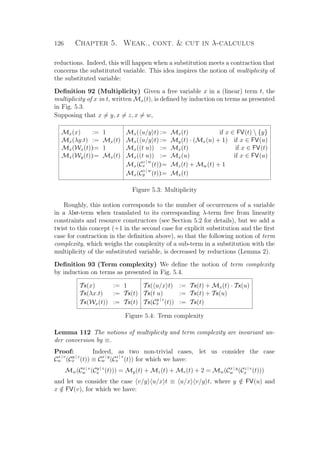
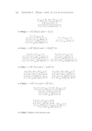
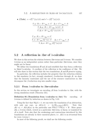
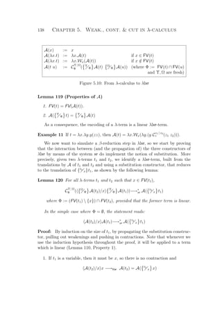
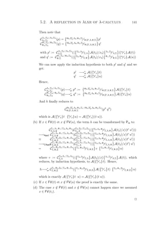
![144 Chapter 5. Weak., cont. cut in λ-calculus
5.2.2 From λlxr-calculus to λ-calculus
In this section we investigate an encoding B from λlxr to λ-calculus, with the
(weak) simulation result (Theorem 121).
Definition 96 (Translation from λlxr to λ-calculus) We define the function
B(t) by induction on the structure of the λlxr-t as shown in Fig. 5.11.
B(x) := x
B(λx.t) := λx.B(t)
B(Wx(t)) := B(t)
B(C
y | z
x (t)) := {x
z}{x
y}B(t)
B(t u) := B(t) B(u)
B( u/x t) := B(u)
x B(t)
Figure 5.11: From λlxr to λ-calculus
Remark that B(t) is not the xr-normal form of t since weakenings and con-
tractions disappear and thus the linearity constraints need not hold anymore.
Lemma 123 (Properties of B) The translation B satisfies the following prop-
erties.
• B( Υ
Φ t) = Υ
Φ B(t)
• FV(B(t)) ⊆ FV(t)
The following result will allow us to project the λlxr-calculus onto the λ-
calculus, as usually done for calculi with explicit substitutions [Ros96].
Lemma 124 (Simulating λlxr-reduction)
1. If t1 ≡ t2, then B(t1) = B(t2).
2. If t1 −→B t2, then B(t1)−→∗
β B(t2).
3. If t1 −→xr t2, then B(t1) = B(t2).
Proof:
1. This is obvious for the equivalence rule Pw. For the other ones we have to
use the substitution lemma (Lemma 40).
2. A B-reduction step at the root of t1 corresponds exactly to a β-reduction
step at the root of B(t1). For the contextual closure, all cases are trivial
except for:](https://image.slidesharecdn.com/frenchenglish-150412084606-conversion-gate01/85/French-english-168-320.jpg)
![148 Chapter 5. Weak., cont. cut in λ-calculus
Lemma 129 The system xr is confluent (and we already know that it is termi-
nating), and the xr-normal form of t is WFV(t)FV(B(t))(A(B(t))).
Proof: By Theorem 116 the system xr is terminating so we can take any
xr-normal form t of t such that t−→∗
xr t . We then have FV(t) = FV(t ) by
Lemma 1 and B(t) = B(t ) by Lemma 124. Since t is an xr-normal form,
t ≡ WFV(t )FV(B(t ))(A(B(t ))) by Theorem 128, so t ≡ WFV(t)FV(B(t))(A(B(t))).
To show confluence let us suppose t−→∗
xr t1 and t−→∗
xr t2. Let us take xr-
normal forms t1 and t2 such that ti−→∗
xr ti. By the previous remark both t1 and
t2 are congruent to WFV(t)FV(B(t))(A(B(t))) which concludes the proof. P
We now establish the reflection. Unfortunately, the shape of the simulation
of β-reduction is not exactly the standard one for a simulation, owing to the
weakenings placed at the top-level that record the free variables that were lost in
the β-reduction. Hence, we use a trick given by O’Conchúir [O’C06] that consists
in generalising the encoding A with a parameter as follows:
Definition 97 (Generalised A) For all finite set S of variables and all λ-term
t such that FV(t) ⊆ S,
AS(t) := WSFV(t)(A(t))
Remark 130 Note that AFV(t)(t) = A(t).
Theorem 131 (Reflection in λlxr of λ-calculus) B and AS form a reflection
in λlxr of the λ-calculus (more precisely, a reflection, in the terms of λlxr whose
free variables are S, of the λ-terms whose free variables are among S).
Proof:
• For the simulation through AS, consider a finite set of variables S. From
Theorem 121, we get that for all λ-term t and u such that FV(t) ⊆ S and
t −→β u the following holds:
AS(t) = WSFV(t)(A(t))
−→+
λlxr WSFV(t)(WFV(t)FV(u)(A(u)))
= WSFV(u)(A(u))
= AS(u)
• The simulation through B is Corollary 125.
• From Remark 127 we get t = B(AS(t)).
• From Lemma 129 we get t−→∗
xr AS(B(t)),
since t−→∗
xr WFV(t)FV(B(t))(A(B(t))) and S = FV(t).
P](https://image.slidesharecdn.com/frenchenglish-150412084606-conversion-gate01/85/French-english-172-320.jpg)
![5.3. Normalisation results 149
We can now derive the confluence property for system λlxr:
Theorem 132 The system λlxr is confluent.
Proof: From Theorems 5 and 131. P
5.3 Normalisation results
In sections 5.1 and 5.2 we have already established the property of subject reduc-
tion, and the reflection in λlxr of λ-calculus. But a calculus which is defined in
order to implement λ-calculus is also expected to satisfy preservation of strong
normalisation (PSN), which we prove in this section.
5.3.1 Preservation of Strong Normalisation
We establish PSN of λlxr by using the simulation technique with a memory op-
erator as presented in Section 4.2. The application of the technique to λlxr can
be summarised as follows:
1. Define a relation H between linear λlxr-terms and λI-terms (Definition 98).
2. Show that −→βπ strongly simulates −→B and weakly simulates −→xr
through H (Theorem 134).
3. Deduce by Corollary 26 that if t H T and T ∈ SNβπ
, then t ∈ SNBxr
.
4. Show that A(t) H i(t) (Theorem 136) and conclude by Theorem 109 the
PSN property (Corollary 137).
We now proceed to develop the above points needed to conclude PSN as
explained above.
Definition 98 The relation H between linear λlxr-terms and λI-terms is in-
ductively defined in Fig. 5.12.
x H x
t H T
λx.t H λx.T
t H T u H U
tu H TU
t H T
N ∈ ΛI
t H [T, N]
t H T u H U
u/x t H U
x T
t H T
Cy | z
x (t) H {x
z}{x
y}T
t H T
x ∈ FV(T)
Wx(t) H T
Figure 5.12: Relation between λlxr λI](https://image.slidesharecdn.com/frenchenglish-150412084606-conversion-gate01/85/French-english-173-320.jpg)
![150 Chapter 5. Weak., cont. cut in λ-calculus
The relation H satisfies the following properties.
Lemma 133 If t H M, then
1. FV(t) ⊆ FV(M)
2. M ∈ ΛI
3. x /∈ FV(t) and N ∈ ΛI implies t H N
x M
4. t ≡ t implies t H M
5. Ψ
Φ t H Ψ
Φ M
Proof: Property (1) is a straightforward induction on the proof tree as well as
Property (2). Properties (3) and (5) are also proved by induction on the tree,
using Lemma 40. For Property (4):
• If Wx(Wy(t)) H M then M = [[T,
−→
Ti ],
−→
Ui] with t H T, y ∈ FV(T) and
x ∈ FV([T,
−→
Ti ]). Then Wy(Wx(t)) H M.
• If v/y u/x t H M with y /∈ FV(u), then M = [ V
y [ U
x T,
−→
Ti ],
−→
Ui]
with t H T, u H U and v H V .
By α-conversion we can assume that x /∈ FV(T1) ∪ . . . ∪ FV(Tm) ∪ FV(V ),
so that M = [ V
y
U
x [T,
−→
Ti ],
−→
Ui] = [ {V
y}U
x
V
y [T,
−→
Ti ],
−→
Ui]. As a
consequence u/x v/y t H M, since by (3) we get u H V
y U.
• Associativity and commutativity of contraction are very similar to the pre-
vious case.
• If u/x C
y | z
w (p) H M, then M = [ U
x [{w
z}{w
y}P,
−→
Pi],
−→
Ui], with p H P
and u H U. We then conclude that C
y | z
w ( u/x p) H M where
M = [{w
z}{w
y} U
x P,
−−−−−→U
x Pi,
−→
Ui].
P
Theorem 134 (Simulation in ΛI)
1. If t H T and t −→xr t , then t H T.
2. If t H T and t −→B t , then there is T ∈ ΛI such that t H T and
T−→+
βπ T .
Proof: By induction on the reduction step. Remark that the case t ∼= t is
already considered by Lemma 133.4 so that we restrict the proof here to basic
reduction steps.](https://image.slidesharecdn.com/frenchenglish-150412084606-conversion-gate01/85/French-english-174-320.jpg)
![5.3. Normalisation results 151
• B: (λx.p) u −→ u/x p.
Then T = [[λx.P,
−→
Pi]U,
−→
Ui] with p H P and u H U. We then obtain the
reduction sequence T−→∗
π [(λx.P)U,
−→
Pi,
−→
Ui] −→β [ U
x P,
−→
Pi,
−→
Ui] = T .
• Abs: u/x (λy.p) −→ λy. u/x p. Then T = [ U
x [λy.P,
−→
Pi],
−→
Ui] with
p H P and u H U. We have T = [λy.( U
x P),
−−−−−→U
x Pi,
−→
Ui].
• App1,App2: Similar to the previous case.
• Var: u/x x −→ u. Then T = [ U
x [x,
−→
Pi],
−→
Ui] with u H U. We have
T = [U,
−−−−−→U
x Pi,
−→
Ui].
• Weak1: u/x Wx(p) −→ WFV(u)(p).
Then T = [ U
x [P,
−→
Pi],
−→
Ui] with p H P, u H U, and x ∈ FV(P). We
have T = [ U
x P,
−−−−−→U
x Pi,
−→
Ui]. Since x /∈ FV(p), then by Lemma 133.3
p H U
x P, and since x ∈ FV(P), FV(U) ⊆ FV( U
x P). By
Lemma 133.1 FV(u) ⊆ FV(U) so FV(u) ⊆ FV( U
x P) concludes the proof.
• Weak2: u/x Wy(p) −→ Wy( u/x p).
Then T = [ U
x [P,
−→
Pi],
−→
Ui] with p H P, u H U, and y ∈ FV(P). We have
T = [ U
x P,
−−−−−→U
x Pi,
−→
Ui] and we still have y ∈ FV( U
x P).
• Cont: u/x C
y | z
x (p) −→ C
Ψ | Υ
Φ ( Υ
Φ u/z Ψ
Φ u/y p).
Then T = [ U
x [{x
z}{x
y}P,
−→
Pi],
−→
Ui] with p H P and u H U. We ob-
tain the following equality T = [ U
z
U
y P,
−−−−−→U
x Pi,
−→
Ui] which can be
expressed as
T = [ Φ
Υ
Φ
Ψ
U
z
U
y P,
−−−−−→U
x Pi,
−→
Ui]
where U = Ψ
Φ U and U = Υ
Φ U. We obtain Ψ
Φ u H U and
Υ
Φ u H U by Lemma 133.5.
• Comp: u/x v/y p −→ u/x v/y p where x ∈ FV(v).
Then T = [ U
x [ Q
y P,
−→
Pi],
−→
Ui] with p H P, v H Q, and u H U.
We have T = [ {U
x}Q
y
U
x P,
−−−−−→U
x Pi,
−→
Ui]. Notice that we obtain
t H U
x P by Lemma 133.3.
• WAbs, WApp1, WApp2, WSubs, Cross are straightforward because the con-
dition x ∈ FV(P) that is checked by Wx(_) is just changed into a side-
condition x ∈ FV(Q) (checked one step later), where x ∈ FV(P) implies
x ∈ FV(Q).](https://image.slidesharecdn.com/frenchenglish-150412084606-conversion-gate01/85/French-english-175-320.jpg)
![152 Chapter 5. Weak., cont. cut in λ-calculus
• Merge: C
y | z
w (Wy(p)) −→ {w
z}p.
Then T = [{w
z}{w
y}[P,
−→
Pi],
−→
Ui] with p H P and y ∈ FV(P). We then
have the equality T = [{w
y}[{w
z}P,
−−−−→
{w
z}Pi],
−→
Ui] and we conclude by
Lemma 133.3.
• CAbs: C
y | z
w (λx.t) −→ λx.C
y | z
w (p).
Then T = [{w
z}{w
y}[λx.P,
−→
Pi],
−→
Ui] with t H P.
We have T = [λx.({w
z}{w
y}P),
−−−−−−−−−→
{w
z}{w
y}Pi,
−→
Ui].
• CApp1, CApp2: Similar to the previous case.
• CSubs: We have C
y | z
w ( u/x p) H [{w
z}{w
y}[ U
x P,
−→
Pi],
−→
Ui] which is equal
to T = [[ {w
z}{w
y}U
x {w
z}{w
y}P,
−−−−−−−−−→
{w
z}{w
y}Pi],
−→
Ui] by Lemma 40. We
have C
y | z
w (u)/x p H T by Lemma 133.3, which concludes this case.
Now for the contextual closure, we use the fact that if P −→βπ P then
U
x P −→βπ
U
x P , and if moreover x ∈ FV(P) and U −→βπ U then
U
x P−→+
βπ
U
x P. The latter is useful for explicit substitutions: if t/x p H Q
and t −→B t , then Q = [ T
x P,
−→
Ui] with p H P, t H T and by the by i.h.we
get T−→+
βπ T such that t H T . Since x ∈ FV(p), x ∈ FV(P) by Lemma 133.1,
and hence Q−→+
βπ [ T
x P,
−→
Ui]. P
Corollary 135 If t H T and T ∈ SNβπ
, then t ∈ SNλlxr
.
Proof: Given that xr is terminating (Lemma 110), it suffices to apply Corol-
lary 26. P
Theorem 136 For any λ-term u, A(u) H i(u).
Proof: By induction on u:
• x H x trivially holds.
• If u = λx.t , then A(t) H i(t) holds by the by i.h. Therefore, we obtain
λx.A(t) H λx.i(t) and λx.Wx(A(t)) H λx.[i(t), x].
• If u = (t u) , then A(t) H i(t) and A(u) H i(u) hold by the i.h. and
Υ
Φ A(t) H Υ
Φ i(t) and Υ
Φ A(u) H Υ
Φ i(u) by Lemma 133-5.
Since Φ
Υ
Υ
Φ i(t) = i(t) (and the same for i(u)), we can then conclude
C
Ψ | Υ
Φ ( Ψ
Φ A(t) Υ
Φ A(u)) H i(t) i(u). P
Corollary 137 (PSN) For any λ-term t, if t ∈ SNβ
, then A(t) ∈ SNλlxr
.
Proof: If t ∈ SNβ
, then i(t) ∈ SNβπ
by Theorems 109 and 108. As A(t) H i(t)
by Theorem 136, then we conclude A(t) ∈ SNλlxr
by Corollary 135. P](https://image.slidesharecdn.com/frenchenglish-150412084606-conversion-gate01/85/French-english-176-320.jpg)
![5.3. Normalisation results 153
5.3.2 Strong normalisation of typed terms
We slightly refine the translation B by lifting all explicit substitutions into B-
redexes (as suggested in [Her95]):
Definition 99 (Refined translation from λlxr to λ-calculus) The function
H(t) is defined by induction in Fig. 5.13.
H(x) := x
H(λx.t) := λx.H(t)
H(Wx(t)) := (λy.H(t)) x
H(C
y | z
x (t)) := (λy.λz.H(t)) x x
H(t u) := H(t) H(u)
H( u/x t) := (λx.H(t)) H(u)
Figure 5.13: From λlxr to λ-calculus
We easily get:
Lemma 138 For all λlxr-term t, A(H(t))−→∗
λlxr t.
Proof: Straightforward induction on t. P
A straightforward induction on typing derivations allows us to show:
Lemma 139 (H preserves types) If t is a λlxr-term such that Γ λlxr t : A,
then Γ λ H(t) : A.
Theorem 140 (Strong normalisation of typed terms) If Γ λlxr t : A then
t ∈ SNB,xr
.
Proof: If Γ λlxr t : A then Γ λ H(t) : A (Lemma 139), so H(t) ∈ SNβ
(Theo-
rem 62). By PSN (Corollary 137) we get A(H(t)) ∈ SNB,xr
. Since A(H(t))−→∗
λlxr t
(Lemma 138), we also have t ∈ SNB,xr
. P](https://image.slidesharecdn.com/frenchenglish-150412084606-conversion-gate01/85/French-english-177-320.jpg)
![154 Chapter 5. Weak., cont. cut in λ-calculus
Conclusion
The calculus λlxr extends the explicit substitution paradigm, in that it features
new constructors in a simple syntax equipped with a natural operational seman-
tics, given by the notion of reduction modulo a set of equations, and further
decomposing β-reduction into more atomic steps.
These constructors represent a tool to analyse and control when sub-terms are
duplicated or erased during computation, thus providing an elegant framework for
studying resource usage or control. This relates to contractions and weakenings
of proof-nets for linear logic [Gir87] to which a sound and complete interpretation
can be defined [KL05, KL07]. From a computational point of view, weakening
constructors are a useful tool to handle garbage collection. Indeed, free variables
are never lost and weakening constructors are pulled out to the top-level during
computation.
In contrast to other HOC in which there is a reflection of λ-calculus, λlxr has
full composition of substitutions and satisfies PSN. It also satisfies confluence and
strong normalisation of simply-typed terms.
It is worth mentioning the calculus obtained by turning the equation Pcs into
a reduction rule (from left to right) and by eliminating reduction rules WSubs
and CSubs satisfies exactly the same properties as the calculus presented in this
chapter, namely Theorems 118,140,121,125,132, and Corollary 137. However,
these rules seem to be necessary for the confluence on open terms (ongoing work).
Many points raised in this work deserve further development. The first one
concerns the study of reduction strategies well-adapted to handle the constructors
for substitution, erasure and duplication. This may take into account the notion
of weak reduction used to implement functional programming [LM99].
Proof techniques used in the literature to show PSN of calculi with explicit
substitutions (zoom-in [ABR00], minimality [BBLRD96], labelled RPO [BG99],
PSN by standardisation [KOvO01], or intersection types) are not all easy to
adapt/extend to reduction modulo and other formalisms. The proof technique
used here seems really flexible.
Using the PSN result, we believe that we can characterise very neatly the
strongly normalising terms of λlxr as the terms typable with intersection types,
as it it the case in λ-calculus as well as in the explicit substitution calculus
λx [LLD+
04].
First-order term syntax for λlxr via de Bruijn indices [dB72], or other special
notation to avoid α-conversion as for example explicit scoping [HvO03] or also
director strings [SFM03], would make implementation easier.
Connections with similar approaches relating graph formalisms to term cal-
culi, as for example that of Hasegawa [Has99] also merits further investigations.](https://image.slidesharecdn.com/frenchenglish-150412084606-conversion-gate01/85/French-english-178-320.jpg)
![Chapter 6
Cut-elimination in G3ii stable
fragments
This chapter tackles the notion of computation in sequent calculus based on
cut-elimination. In a way similar to a survey, it presents traditional ideas in a uni-
fied framework, using the traditional sequent calculus G3ii and its corresponding
HOC of proof-terms called λG3 and presented in Chapter 2.
Starting from the admissibility of the cut-rule in G3ii, we use our framework
with terms called λG3 to relate inductive proofs of term-irrelevant admissibility to
rewrite systems that eliminate the cut-constructor. These systems in fact make
sense even without the notion of typing for λG3, although we do need typing
to prove their strong normalisation. We identify the structure of such rewrite
systems that perform cut-elimination in a typed framework, in that they are made
of a kernel that reduces principal cuts/cut constructors and propagation systems
which may vary. In this generic framework we show the critical pairs of these
systems, which can be solved in two canonical ways leading to the introduction
of a generic notion of CBN and CBV sub-systems. We present three kinds of
propagation system with a comparative approach, essentially by investigating
their ability to simulate β-reduction through Gentzen’s or Prawitz’s encodings
described in Chapter 2. We also compare the CBN and CBV equational theories
that these propagation systems produce.
We then show two restrictions on λG3-terms and their typing rules that corre-
spond to the sequent calculi LJT and LJQ [Her95], and show that these restrictions
are respectively stable under the CBN and CBV sub-systems, which become their
natural cut-elimination procedures. Two simple purification rules, reducing arbi-
trary terms of λG3 to terms of these restrictions, show the completeness of the
two fragments.
We recall the strong connection between LJT, the λ-calculus and the λ-
calculus, by means of a reflection based on Prawitz’s encoding. We also give
a new proof of the PSN property for λ, as another illustrative example of the
safeness and minimality technique.
155](https://image.slidesharecdn.com/frenchenglish-150412084606-conversion-gate01/85/French-english-179-320.jpg)
![156 Chapter 6. Cut-elimination stable fragments
We then investigate LJQ, described as the typing system of a term syn-
tax, which we then use to establish a connection with the CBV calculus λC of
Moggi [Mog88]. A preliminary version of this work has been published in [DL06].
6.1 Cut-elimination
6.1.1 Aims
The main property of G3ii is that the cut-rule is admissible in the cut-free system,
so for any derivation using cuts there exists a derivation of the same logical
sequent. As described in Chapter 2, this corresponds, in the framework of λG3
with terms, to the term-irrelevant admissibility of the cut-rule in the rest of the
system.
Usually, admissibility of a rule in sequent calculus is proved by induction, for
instance on derivations of the premisses. The very same argument can be used to
prove term-irrelevant admissibility, in a canonical typed HOC that corresponds
to the sequent calculus. Moreover, it defines a process that transforms a term M
that uses the constructor typed by the rule into another term M , with the same
type in the same environment, that does not use this constructors.
The process given by the induction is in fact a notion of reduction given by
an innermost strategy in a rewrite system that specifies how to eliminate the
constructor in the following sense:
Property 141
141.1 A term containing the constructor is reducible (all cases are covered by the
induction).
141.2 The rewrite system satisfies the subject reduction property.
141.3 The innermost strategy given by the inductive argument terminates, using
the induction measure.
This gives a notion of reduction in the typed HOC that is weakly normalising
(from point 3). This suffices to prove term-irrelevant admissibility, but for a gen-
eral notion of computation we often want a strong normalisation property. And
in fact it is often the case that the induction measure that proves termination of
the innermost strategy also proves the strong normalisation of general reduction.1
This applies to G3ii and λG3, in that the admissibility of cut gives rise to a
cut-elimination process. In the framework of λG3, this can be done by means of
a rewrite system, cut-free proofs being thus denoted by terms in normal form.
1
Strong normalisation can actually be directly inferred from weak innermost normalisation
in the particular case of orthogonal first-order systems [O’D77]](https://image.slidesharecdn.com/frenchenglish-150412084606-conversion-gate01/85/French-english-180-320.jpg)
![6.1. Cut-elimination 157
Various such reduction systems are given in the literature, but their diversity
is striking. Whilst this might be explained by the diverse requirements that the
systems fulfil on top of the above properties, choices of design are often given little
justification. They might aim at simplicity, strong normalisation, confluence,
simulation of β-reduction. . .
Here we try to cover various reduction systems achieving cut-elimination, in
the prospect of showing connections between proof theory and computer science,
especially rewriting and (functional) programming. We thus express these sys-
tems with two (diverging) concerns:
• formulating them as general, unrestricted, and simple as we can without
breaking strong normalisation,
• partitioning and restricting them only to give them semantical meaning, in
effect relating them to CBV and CBN semantics.
Proving strong normalisation of the cut-reduction system inferred from in-
ductive proofs of cut-admissibility such as that of [Gen35] is often simpler than
proving strong normalisation of typed λ-calculus (this was in fact the motivation
of [Gen35] for introducing sequent calculus). This is true until cut-reduction is
able to strongly simulate β-reduction. Indeed, a criterion on which we compare
the various systems expressed with the above concerns is their computational
strength, how they simulate, or more generally how they relate to, β-reduction.
Finally, we choose to base those systems on λG3 as it is the most natural
framework without, for instance, adding to the syntax extra constructors -and
typing rules- as in [Her94, EFP06], until Chapter 7 where the G4ii-calculus re-
quires a particular treatment.
6.1.2 Kernel propagation system
Despite their diversity, all the cut-elimination systems have to deal with those
basic cases when the cut-type is principal in both premisses. In these cases
the inference rules provide canonical ways of reducing the cut, possibly creating
cuts on sub-formulae. These cuts are sometimes called logical cuts [Urb00], or
principal cuts. At the level of terms, they correspond to the constructs N † x.M
where N is a value and M is an x-covalue, which we call logical cut-constructor
or principal cut-constructor. Fig. 6.1 shows the standard rewrite rules to reduce
them. We denotes the reduction relation −→princs
.
What is less standard is the way to deal with those cases in which the cut-type
is not principal in at least one premiss. What process will reduce the problem
to the case of principal cuts? It clearly depends on the proof of the premiss
in which the cut-formula is not principal, pushing the cut thereinto, and can
disregard the proof of the other premiss. But then if in both premisses the cut-
type is not principal, a choice has to be made, leading to non-confluence of the](https://image.slidesharecdn.com/frenchenglish-150412084606-conversion-gate01/85/French-english-181-320.jpg)
![158 Chapter 6. Cut-elimination stable fragments
B λx.M † y.y[N, z.P] −→ N † x.M † z.P if y /∈ FV(P) ∪ FV(N)
x † y.y[N, z.P] −→ x[N, z.P] if y /∈ FV(P) ∪ FV(N)
λx.M † y.y −→ λx.M
x † y.y −→ x
Figure 6.1: Principal cut-reductions
process unless it is restricted by a general preference (or strategy) that determines
each of these choices. It is interesting to see that this non-confluence can even
occur in the intuitionistic sequent calculus, whilst it is often thought to be a
specificity of classical logic.
Cut-elimination systems thus reduce non-principal cuts with rules based on
two kinds of behaviour: left-propagation, denoted −→left , reduces a cut by push-
ing it to the left, depending on the proof of its first premiss (in which the cut-
type is not principal), while right-propagation, denoted −→right , reduces a cut by
pushing it to the right depending on the proof of its second premiss (in which the
cut-type is not principal). The former reduces N † x.M depending on N that
is not a value (in other words, it alleviates the body N of the cut-constructor, re-
gardless of M), and the latter reduces it depending on M that is not an x-covalue,
regardless of N.
Clearly, the two situations overlap when neither N is a value nor M is an
x-covalue, or, in a typed framework, when in neither premisses of the cut the
cut-type is principal. This generates critical pairs and non-confluence, and an
interesting point is that techniques to avoid this situation (namely, deciding which
kind of rule will apply with priority) reveal connections with the CBV and CBN
semantics of functional programming, as introduced in Chapter 3. Thus, always
giving preference to left-propagation corresponds to CBV, while preference to the
right-propagation corresponds to CBN, which we define as follows:
Definition 100 (CBV CBN sub-systems)
• The CBN-sub-system restricts the left-propagation system by requiring it
to reduce N † x.M only when M is an x-covalue (and thus the cut-
constructor cannot be right-propagated).
We write −→CBNs for the reduction relation generated by −→princs
, −→right ,
and this restricted −→left .
• The CBV-sub-system restricts the right-propagation system by requiring it
to reduce N † x.M only when N is a value (and thus the cut-constructor
cannot be left-propagated).
We write −→CBVs for the reduction relation generated by −→princs
, −→left ,
and this restricted −→right .](https://image.slidesharecdn.com/frenchenglish-150412084606-conversion-gate01/85/French-english-182-320.jpg)
![6.1. Cut-elimination 159
Now, obtaining the completeness of these restrictions for cut-elimination also
justifies the need for a general strong normalisation result of the whole system
rather than weak normalisation.
Finally, variations of the principal rules are of interest. When in one of the
premisses of a principal cut, the cut-type is introduced by an axiom, the standard
way to eliminate the cut is to only keep the proof of the other premiss (possibly
using a contraction if the axiom proves the first premiss). But this works in fact
whether or not the cut-type is principal in this other premiss, and it thus applies
to cuts that might not be logical as well. This generalises the scope of principal
rules, the reduction relation of which we denote −→princ , but it also simplifies
them as shown in Fig 6.2.
B λx.M † y.y[N, z.P] −→ N † x.M † z.P if y /∈ FV(P) ∪ FV(N)
B1 x † y.N −→ {x
y}N
B2 M † y.y −→ M
Figure 6.2: Generalised principal reductions
We define −→CBV and −→CBN just like −→CBVs and −→CBNs , but consider-
ing −→princ instead of −→princs
.
Convenient and simplifying though this extension is, it creates new critical
pairs with the left and right propagation (making confluence of −→CBV and
−→CBN more difficult to prove).
In the next section we present three kinds of propagation rules, respectively
generating systems SI, KK and JC, for which we have
(←→∗
CBVKKs
) = (←→∗
CBVKK
) = (←→∗
CBVJCs
) = (←→∗
CBVJC
)
(←→∗
CBNKKs
) = (←→∗
CBNKK
) = (←→∗
CBNJCs
) = (←→∗
CBNJC
)
We call those equational theories ≡CBV and ≡CBN. In system SI, we only have in
general
(←→∗
CBVSIs
) ⊆ (←→∗
CBVSI
) ⊆ (≡CBV)
(←→∗
CBNSIs
) ⊆ (←→∗
CBNSI
) ⊆ (≡CBN)
However, on weakly normalising terms we also have
(←→∗
CBVSIs
) = (←→∗
CBVSI
) and (←→∗
CBNSIs
) = (←→∗
CBNSI
). On strongly normal-
ising terms, in particular for typed terms, we even have
(←→∗
CBVSIs
) = (←→∗
CBVSI
) = (≡CBV) and (←→∗
CBNSIs
) = (←→∗
CBNSI
) = (≡CBN).
6.1.3 Instances of propagation systems
Simple propagation - System SI
We present in Figure 6.3 perhaps the simplest rewrite systems for left and right
propagation, respectively denoted −→leftSI
and −→rightSI
. We call SI (resp. SIs)](https://image.slidesharecdn.com/frenchenglish-150412084606-conversion-gate01/85/French-english-183-320.jpg)
![160 Chapter 6. Cut-elimination stable fragments
the system with these rules and those of princ (resp. of princs).
left1 z[N, y.P] † x.M −→ z[N, y. P † x.M ]
right1 N † x.y −→ y
right2 N † x.(λy.M) −→ λy. N † x.M
right3 N † x.x[M, z.P] −→ N † x.x[ N † x.M , z. N † x.P ]
if x ∈ FV(M) ∪ FV(P)
right4 N † x.x [M, z.P] −→ x [ N † x.M , z. N † x.P ]
Figure 6.3: SI-propagation
Notice that in rule right3, the side-condition x ∈ FV(M) ∪ FV(P) comes
from our requiring the term, to which the cut-constructor is applied, to not
be an x-covalue. Otherwise, the rule could be re-applied indefinitely, although
termination could be alternatively recovered by applying the rule only before rule
B as follows:
λx.M † y.y[N, z.P] −→ λx.M † y.N † x.M † z. λx.M † y.P
The whole system remains complete for cut-elimination, but it intermingles the
three rewrite systems in a way that obscures the connection with CBV and CBN,
which we want to reveal formally. We therefore keep the side-condition.
The reduction relation −→SI can easily be proved satisfying Properties 141.1
and 141.2 (subject reduction). Now we consider normalisation:
Theorem 142 (Strong Normalisation)
1. −→SIB is strongly normalising.
2. If Γ λG3 M :A then M ∈ SNSI
.
Proof: Both results can be proved using a LPO based on the following infinite
first-order signature and its precedence relation:
sub(_, _) cut(_, _) ii(_, _) i(_)
We define the following encoding:
x :=
λx.M := i(M)
x[N, y.M] := ii(N, M)
N † y.M := cut(N, M) if M is a y-covalue
N † y.M := sub(N, M) otherwise
All the rules but B decrease the encoding. In the typed case, we refine the above
precedence relation by
subB
(_, _) cutB
(_, _) · · · subA
(_, _) cutA
(_, _) ii(_, _) i(_)](https://image.slidesharecdn.com/frenchenglish-150412084606-conversion-gate01/85/French-english-184-320.jpg)
![6.1. Cut-elimination 161
if type B A. We now refine the above encoding: technically, it is now defined
on the typing trees (and the proof of subject reduction shows how the rules
transform the trees), although we abusively express the encoding from the proof-
term:
x :=
λx.M := i(M)
x[N, y.M] := ii(N, M)
N † y.M := cutA
(N, M) if M is a y-covalue
N † y.M := subA
(N, M) otherwise
where A is the cut-formula. Now rule B decreases the encoding as well as the
other rules. P
Now we state a few properties about the CBV and CBN relations :
Theorem 143 (Confluence)
1. −→CBNSIs
and −→CBVSIs
are confluent.
2. We conjecture that −→CBNSI
and −→CBVSI
are confluent.
Proof:
1. The left and right propagation systems are orthogonal higher-order rewrite
systems, and hence, so are −→CBNSIs
and −→CBVSIs
, which entails conflu-
ence (see e.g. [Ter03]).
2. We could either try the method of parallel reduction (see e.g. [Tak89])
or establish that a CPS-translation forms a pre-Galois connection with a
confluent fragment of λ-calculus (as in Chapter 3).
P
Lemma 144 Provided the terms are weakly normalising,
1. x † y.M ←→∗
CBVSIs
{x
y}M and x † y.M ←→∗
CBNSIs
{x
y}M,
2. M † y.y ←→∗
CBVSIs
M and M † y.y ←→∗
CBNSIs
M.
Proof: We first prove it for M ∈ λG3cf
by structural induction on M. Then
for an arbitrary M we first reduce it using Property 141.1, to a M ∈ λG3cf
for
which the statement holds. P
Theorem 145 (Equational theories) On weakly normalising terms,
(←→∗
CBVSIs
) = (←→∗
CBVSI
) and (←→∗
CBNSIs
) = (←→∗
CBNSI
).
Proof: This is a direct corollary. P](https://image.slidesharecdn.com/frenchenglish-150412084606-conversion-gate01/85/French-english-185-320.jpg)
![162 Chapter 6. Cut-elimination stable fragments
Now we prove a lemma about commutation of cuts, that will later be used to
relate the equational theories of system SI to those of richer propagation systems.
Lemma 146 Provided N † x.M is strongly normalising, we have
P † y. N † x.M ←→∗
CBNSI
P † y.N † x. P † y.M
P † y. N † x.M ←→∗
CBVSI
P † y.N † x. P † y.M if P is a value
N † x.M † y.P ←→∗
CBNSI
N † x. M † y.P if P is a y-covalue
N † x.M † y.P ←→∗
CBNSI
N † x. M † y.P
Proof: By induction on the length of the longest reduction sequence reducing
N † x.M . If N ∈ λG3cf
or M ∈ λG3cf
we can reduce it and the induction
hypothesis applies. If both are in λG3cf
then N † x.M is the redex of a rewrite
rule and then it is a case analysis on the rule. P
A richer propagation - System KK
Simple though it is, the above propagation system does not make cut-elimination
powerful enough to simulate β-reduction. Consider the reduction
M = (λx.(λx1.x) x2) λy.y −→β (λx1.λy.y) x2 = N. We have
G2
(M) = Pr(M) = λx. λx1.x † z3.z3[x2, z4.z4] † z1.z1[λy.y, z2.z2]
−→∗
SI λy.y † x. λx1.x † z3.z3[x2, z4.z4]
but then we are stuck, because all we could do before propagating the cut we
want is reduce the inner cut first, which encodes the β-redex that remains in N
and which we still therefore need.
Whether λ-calculus is encoded via Gentzen’s or Prawitz’s translation, a β-
redex is encoded using a cut, and a substitution is implementing by reducing and
propagating a cut. Hence, since substitutions can instantiate variables through
a β-redex, cut should be propagated through cuts. However, a permutation of
cuts such as N † x. M † y.P −→ N † x.M † y. N † x.P would fail to be
terminating. Variations on that problem can be found in works tackling the
notion of composition in explicit substitution calculi such as λx [BR95], already
mentioned in Chapters 4 and 5.
However, [Kik04b, Kik06] noticed that arbitrary permutations were not nec-
essary for the simulation, but only specific ones. Following his ideas, the permu-
tation rules of Fig 6.4 enable the simulation of β-reduction.
We call KK (resp. KKs) the system with these rules and those of princ (resp.
with princs).
Remark 147 If all cut-constructors in N are logical and x ∈ FV(N) then
N † x.N −→CBNKK
N and V † x.N −→CBVKK
N.](https://image.slidesharecdn.com/frenchenglish-150412084606-conversion-gate01/85/French-english-186-320.jpg)
![6.1. Cut-elimination 163
left2 λz.M † y.y[P, z .Q] † x.N
−→ λz.M † y.y[P, z . Q † x.N ]
if y ∈ FV(P) ∪ FV(Q)
right5 N † x. λz.M † y.y[P, z .Q]
−→ λz. N † x.M † y.y[ N † x.P , z . N † x.Q ]
if y ∈ FV(P) ∪ FV(Q)
Figure 6.4: Additional rules for KK-propagation
Lemma 148
1. All cuts in Pr(M) and Prx.N (M1 M2) are logical (provided all cuts in N
are). This is a major difference with Gentzen’s encoding.
2. If N −→CBNKKs
N then Prx.N (M1 M2) −→CBNKKs
Prx.N (M1 M2) and
if N −→CBVKKs
N then Prx.N (M1 M2) −→CBVKKs
Prx.N (M1 M2).
3. If N is a y-covalue, then
Prx.N (M1 M2) † y.N −→∗
CBNKKs
Prx. N †y.N (M1 M2) and
Pr(M1 M2) † y.N −→∗
CBNKKs
Pry.N (M1 M2).
4. We then have Pr(M ) † x.Pr(M) −→∗
CBNKKs
Pr( M
x M) and
Pr(V ) † x.Pr(M) −→∗
CBVKKs
Pr( V
x M).
Proof: Each of the above points is obtained by straightforward inductions on M
and M1 M2. For the last point the induction also requires the auxiliary property
that if all cut-constructors in N are logical, the following holds:
if x ∈ FV(N), then
Pr(M ) † x.Pry.N (M1 M2) −→∗
CBNKKs
Pry. Pr(M )†x.N ( M
x (M1 M2)) and
Pr(V ) † x.Pry.N (M1 M2) −→∗
CBVKKs
Pry. Pr(V )†x.N ( V
x (M1 M2))
otherwise, Pr(M ) † x.Pry.N (M1 M2) −→∗
CBNKKs
Pry.N ( M
x (M1 M2)) and
Pr(V ) † x.Pry.N (M1 M2) −→∗
CBVKKs
Pry.N ( V
x (M1 M2)). P
Theorem 149 (Simulation of β-reduction)
−→KKs strongly simulates −→β through Prawitz’s translation. More precisely,
1. If M −→β M then Pr(M)−→+
CBNKKs
Pr(M ).
2. If M −→βV
M then Pr(M)−→+
CBVKKs
Pr(M ).
where βV is the reduction rule of the λV-calculus (see Chapter 3).](https://image.slidesharecdn.com/frenchenglish-150412084606-conversion-gate01/85/French-english-187-320.jpg)
![164 Chapter 6. Cut-elimination stable fragments
Proof: By induction on the derivation of the reduction step, using the lemma
above. If M −→β M then Pr(M)−→+
CBNKKs
Pr(M ) and if M1 M2 −→β M1 M2
Pry.N (M1 M2)−→+
CBNKKs
Pry.N (M1 M2), which are proved by induction on the
derivation step, using the above lemma. This is a minor variant of the proof
in [Kik06]. Point 2 is proved similarly. P
The reduction relation −→KK still satisfies Property 141.1 because it extends
−→SI . For Property 141.2 (subject reduction), it suffices to check the two new
rules, which is straightforward.
As for Property 141.3, we only conjecture the strong normalisation of typed
terms:
Conjecture 150 (Strong Normalisation) If Γ λG3 M :A then M ∈ SNKK
.
Since the calculus simulates β-reduction, proving this conjecture is at least as
hard as the strong normalisation of the simply-typed λ-calculus. However what
we can do now is prove the strong normalisation of the system without rule B:
it suffices to refine the first encoding from the proof of Theorem 142 as shown in
Fig. 6.5.
x :=
λx.M := i(M)
x[N, y.M] := ii(N, M)
N † y.M := cut(N, M) if M is a y-covalue
N † y.M := sub(N, M) otherwise
Figure 6.5: Encoding of λG3 into a first-order syntax
Lemma 151 If M −→KKB N then MN. Hence, −→KKB is terminating.
Proof: It suffices to check all the rules. P
The conjecture above is motivated by the fact that in rules left2 and right5,
the outer cut, which is not principal, is pushed through a principal cut. In other
words, the property for a cut of being principal is preserved by reduction and can
be used as a flag (as in Fig. 6.5) whose state can only evolve in one direction.
Note that the simulation works with Prawitz’s encoding because cuts are
only used to encode β-redexes and are thus principal. In Gentzen’s encoding
where a potentially non-principal cut-constructor encodes each application, the
simulation fails. In fact, the original system of [Kik06] is rather like the rules
below (although the first one is restricted to the case when N is an x-covalue](https://image.slidesharecdn.com/frenchenglish-150412084606-conversion-gate01/85/French-english-188-320.jpg)
![6.1. Cut-elimination 165
different from x):
M † y.P † x.N −→ M † y. P † x.N
if M † y.P is a principal cut-constructor
N † x. M † y.P −→ N † x.M † y. N † x.P
if M † y.P is a principal cut-constructor
Those rules are simpler, and in case we consider other connectives than impli-
cation, they suffice, otherwise we would need as many rules left2 and right5 as
connectives, i.e. one for each pair of dual constructors for the left and right in-
troduction.
However, the cut-constructor at the root of the right-hand side of the rules
above is no longer a principal cut-constructor. It could become one again if the
cut-constructor that has come in-between were pushed one step further (as in
left2 and right5). Hence, in presence of non-determinism, a change of strategy can
occur precisely after applying the above rules, so this version seems more difficult
to prove strongly normalising than the previous one (however, the restriction
of [Kik06] about N in the first rule above might reduce the difficulty of proving
strong normalisation).
Again, we conjecture the confluence of the CBV- and CBN-reduction.
Conjecture 152 (Confluence) Both −→CBNKK
and −→CBVKK
are confluent.
And again we could either try the method of parallel reduction (see e.g. [Tak89])
or establish that a CPS-translation forms a pre-Galois connection with a confluent
fragment of λ-calculus (as in Chapter 3).
Lemma 153
x † y.M ←→∗
CBVKKs
{x
y}M (resp. x † y.M ←→∗
CBNKKs
{x
y}M) and
M † y.y ←→∗
CBVKKs
M (resp. M † y.y ←→∗
CBNKKs
M).
Proof: We first prove it in the case when M is a normal form for system
−→KKB , that is to say, when all its cut-constructors are logical. With the two
new rules left2 and right5 of system KK, the above terms are all redexes of KK B
(this is why this theorem might not hold for system SI), hence we can prove this
by induction on M.
Then for an arbitrary M we first reduce it, using Lemma 151, to a term M
that is a normal form for −→KKB , and for which the statement holds. P
Corollary 154 (Equational theories)
1. (←→∗
CBVSI
) ⊆ (←→∗
CBVKK
) and (←→∗
CBNSI
) ⊆ (←→∗
CBNKK
).
2. (←→∗
CBVKKs
) = (←→∗
CBVKK
) and (←→∗
CBNKKs
) = (←→∗
CBNKK
).](https://image.slidesharecdn.com/frenchenglish-150412084606-conversion-gate01/85/French-english-189-320.jpg)
![166 Chapter 6. Cut-elimination stable fragments
Proof: The first point is straightforward. The second is a consequence of the
above lemma. P
Remark 155 Note that on terms that are in SNSI
, we can infer from Lemma 146
that (←→∗
CBVKK
) = (←→∗
CBVSI
) and (←→∗
CBNKK
) = (←→∗
CBNSI
).
The simulation of λ-calculus only works with Prawitz’s encoding because only
logical cuts lie in the encoding. We shall also see that Prawitz’s encoding will need
to be modified to be adapted to the call-by-value discipline, in a way that creates
non-principal cuts. Hence, we shall need propagation systems more powerful than
KK that allow propagation of cuts through any kind of cut.
Urban’s jumping cuts - System JC
One of the purposes of this chapter being to relate cut-elimination to normalisa-
tion in λ-calculus, we present an alternative (more powerful) propagation system.
This idea comes from Christian Urban [Urb00]: a cut “jumps” to the places where
the cut-formula is principal, as shown in the right-propagation system of Fig 6.6.
left N † x.M −→ {N † x.M} if N is not a value
right N † x.M −→ N †x.M if M is not an x-covalue
where {N † x.M} and N †x.M are constructions defined as follows:
{y † x.N} := {y
x}N
{λy.M † x.N} := λy.M † x.N
{z[M, y.P]† x.N} := z[M, y. {P † x.N}]
{ M † y.P † x.N} := M † y.{P † x.N}
N †x.x := N
N †x.y := y
N †x.(λy.M) := λy. N †x.M
N †x.x[M, z.P] := N † x.x[ N †x.M , z. N †x.P ]
N †x.x [M, z.P] := x [ N †x.M , z. N †x.P ]
N †x. M † y.P := N †x.M † y. N †x.P
Figure 6.6: JC-propagation
Alternatively, one could introduce {_† _._} and _ †_._ as constructors
of the syntax of proof-terms (with the same typing rule as that of _ † _._ ), and
turn the above definitions into sets of rewrite rules, oriented from left to right,
that eliminate the two constructors.
The rewrite rule corresponding to the last line of each definition would then
not be needed for completeness of the cut-elimination process, as the inner cut
could be eliminated first. However, this commutation of cuts is precisely what](https://image.slidesharecdn.com/frenchenglish-150412084606-conversion-gate01/85/French-english-190-320.jpg)
![6.1. Cut-elimination 167
makes the simulation of β-reduction possible (as in system KK), as does the
version written above, with {_† _._} and _ †_._ considered as construc-
tions, rather than constructors. Indeed, both versions can reduce the external
substitution in N † x. P † y.R while the simple system cannot.
Although the version with the explicit operator is also proved terminating on
typed terms, we shall stick to the version presented above, as it avoids extending
the syntax and more closely relates to λ-calculus, which uses the construction of
substitution.
Theorem 156 (Strong Normalisation)
1. −→JCB is strongly normalising.
2. If Γ λG3 M :A then M ∈ SNJC
.
Proof: This is simply the intuitionistic restriction of the system of [Urb00],
which is proved strongly normalising. P
Again, we conjecture the confluence of the CBV- and CBN-reduction.
Conjecture 157 (Confluence) Both −→CBNJC
and −→CBVJC
are confluent.
And again we could either try the method of parallel reduction (see e.g. [Tak89])
or establish that a CPS-translation forms a pre-Galois connection with a confluent
fragment of λ-calculus (as in Chapter 3).
Again, we show that the enhanced cut-elimination is consistent with the sim-
ple one in the following sense:
Theorem 158 (Equational theories 1)
(←→∗
CBVJCs
) = (←→∗
CBVJC
) and (←→∗
CBNJCs
) = (←→∗
CBNJC
)
Proof: System JCs simulates system JC. P
Theorem 159 (Equational theories 2)
1. We have
(←→∗
CBVKK
) = (←→∗
CBVJC
)
(←→∗
CBNKK
) = (←→∗
CBNJC
)
2. Note that on terms that are in SNSI
,
(←→∗
CBVSI
) = (←→∗
CBVJC
)
(←→∗
CBNSI
) = (←→∗
CBNJC
)
Proof: System KK B can reduce any term to a term in which all cut-
constructors are principal. Now for terms that satisfy this property, rules left2
and right5 of system KK are just as powerful as the reduction in JC that use
{_† _._} and _ †_._ . The second point is then a corollary of Remark 155.
P](https://image.slidesharecdn.com/frenchenglish-150412084606-conversion-gate01/85/French-english-191-320.jpg)
![168 Chapter 6. Cut-elimination stable fragments
6.2 T-restriction LJT
6.2.1 A fragment of λG3
We call t-restriction of λG3 the fragment of CBN-pure terms defined as follows:
Definition 101 (CBN-purity) A term is CBN-pure if in any sub-term of the
form x[M, y.N], N is a y-co-value.
Theorem 160 (Preservation of CBN-purity) CBN-reduction preserve CBN-
purity.
Proof: Easy check on the rules. P
Now we prove that the t-restriction is logically complete. We show that any
proof can be transformed into a CBN-pure term, and we use for that the following
purification rule:
(CBN − pur) x[M, y.N] −→ x[M, z.z] † y.N if N is not a y-covalue
Note that this rule satisfies the subject reduction property. It also terminates,
simply because every application of this rule deceases the number of sub-terms
of the form x[M, y.N] with N not a y-covalue.
Theorem 161 (Prawitz’s encoding produces CBN-pure terms)
Prawitz’s encoding only produces CBN-pure terms of λG3, that is, for every λ-
term t, Pr(t) is CBN-pure.
Proof: This is proved by induction on t, together with the fact that if N is an
x-covalue that is CBN-pure, then Prx.N (t1 t2) is CBN-pure. P
This is an important remark since it already suggests a strong connection between
the t-fragment and λ-calculus.
From a logical point of view, the t-restriction corresponds to the sequent
calculus LJT, as defined for instance in [Her95]. The t-restriction can also be
expressed by separating explicitly the covalues from the other terms, with a
syntactic category for covalues, that is to say, for x-covalues, abstracting on x:
M, N, P ::= λx.M | x l | M † x.N
l ::= [] | M · l
The constructor [] can be seen as representing the higher-order term x.x and M ·l
can be seen as representing x.x[M, y.N] if l represents y.N with
x ∈ FV(M) ∪ FV(N).
The reduction rules are simply inherited from the CBN-reductions of λG3.
The typing rules are also inherited from λG3, as shown in Figure 6.7.](https://image.slidesharecdn.com/frenchenglish-150412084606-conversion-gate01/85/French-english-192-320.jpg)
![6.2. T-restriction LJT 169
Γ; A [] : A
Γ M :A Γ, x : A N :B
Γ M † x.N :B
Γ M :A Γ; B l : C
Γ; A→B M · l : C
Γ, x : A M :B
Γ λx.M :A→B
Γ, x : A; A l : B
Γ, x : A x l:B
Figure 6.7: LJT
6.2.2 The λ-calculus
This calculus is (almost) that of [Her95] called λ, whose syntax turns the con-
structions {_† _._} and _ †_._ into constructors _@_ and _/_ _, re-
spectively. The syntax of λ is thus:
Definition 102 (Syntax of λ)
M, N ::= λx.M | x l | M l | M/x N
l, l ::= [] | M · l | l@l | M/x l
λx.M and N/x M bind x in M, and M/x l binds x in l.
The reduction rules of λ are defined in Figure 6.8, the typing rules are defined
in Figure 6.9. They inductively define the derivability of three kinds of sequents:
some of the form Γ M :A and some of the form Γ; B l:A. In the latter case,
B is said to be in the stoup of the sequent, according to a terminology due to
Girard. Derivability in λ of the two kinds of sequents is denoted Γ λ
M :A, and
Γ; B λ
l:A, respectively.
Many variants of λ can be defined (such as the one in Fig. 6.7), depending
on whether we prefer constructors or constructions, in particular whether we
consider explicit or implicit substitutions. A comprehensive study of the variants
for the t-restriction can be found in [Esp02].
6.2.3 A reflection of (CBN) λ-calculus
In this section we establish a strong connection between λ (or the t-fragment of
λG3) and λ-calculus, whose unrestricted notion of computation can be considered
as the CBN-λ-calculus.
Indeed, the example of λ is a typical case where the syntax does not include
that of λ-calculus, but the latter can be encoded in it, since Prawitz’s encoding](https://image.slidesharecdn.com/frenchenglish-150412084606-conversion-gate01/85/French-english-193-320.jpg)
![170 Chapter 6. Cut-elimination stable fragments
B (λx.M) (N · l) −→ ( N/x M) l
System x:
B1 M [] −→ M
B2 (x l) l −→ x (l@l )
B3 (M l) l −→ M (l@l )
A1 (M · l )@l −→ M · (l @l)
A2 []@l −→ l
A3 (l@l )@l −→ l@(l @l )
C1 P/y λx.M −→ λx. P/y M
C2 P/y (y l) −→ P P/y l
C3 P/y (x l) −→ x P/y l
C4 P/y (M l) −→ P/y M P/y l
D1 P/y [] −→ []
D2 P/y (M · l) −→ ( P/y M) · ( P/y l)
D3 P/y (l@l ) −→ ( P/y l)@( P/y l )
Figure 6.8: Reduction rules for λ
Γ; A l:B (x : A) ∈ Γ
selectx
Γ x l:B
ax
Γ; A []:A
Γ, x:A M :B
→ r
Γ λx.M :A→B
Γ M :A Γ; B l:C
→ l
Γ; A→B M · l:C
Γ M :A Γ; A l:B
cut3
Γ M l:B
Γ; C l :A Γ; A l:B
cut1
Γ; C l @l:B
Γ P :A Γ, x:A M :C
cut4
Γ P/x M :C
Γ P :A Γ, x:A; B l:C
cut2
Γ; B P/x l:C
Figure 6.9: Typing rules for λ
only produces CBN-pure terms of λG3 (Theorem 161). Hence we can reformulate
the latter with the syntax of λ, we do in Figure 6.10.
Fig. 6.11 reformulates, in the case of λ, Gentzen’s encoding from λG3 to λ-
calculus (see Chapter 2).
Now we show that B and A form a reflection in λ of λ-calculus. We first prove
the following results:](https://image.slidesharecdn.com/frenchenglish-150412084606-conversion-gate01/85/French-english-194-320.jpg)
 otherwise
Al(t u) := AA(u)·l(t)
Al(x) := x l
Al(t) := A(t) l otherwise
Figure 6.10: From λ-calculus to λ
B(λxA
.M) := λxB(A)
.B(M)
B(x l) := {x
z}Bz
(l)
B(M l) := B(M)
z Bz
(l)
B( P/x M) := B(P)
x B(M)
By
([]) := y
By
(M · l) := y B(M)
z Bz
(l)
By
(l@l ) := By(l)
z Bz
(l )
By
( P/x l) := B(P)
x By
(l)
Figure 6.11: From λ to λ-calculus
Lemma 162
1. A(t) and Al(t) are always x-normal forms (provided l is).
2. If l −→Bx l then Al(t) −→Bx Al (t).
3. Al (t) l−→∗
x Al @l(t) and A(t) l−→∗
x Al(t).
4. A(u)/x A(t)−→∗
x A({u
x}t) and A(u)/x Al(t)−→∗
x A A(u)/x l({u
x}t).
Proof: Each of the above points is obtained by straightforward inductions on
t. P
Now we study the composition of the two encodings:
Lemma 163 Suppose M and l are x-normal forms.
1. If t = x or t = t1 t2 or l = [], then Al(t) = A({t
x}Bx
(l)) if x /∈ FV(l).
2. M = A(B(M)).
Proof: By simultaneous induction on l and M. P](https://image.slidesharecdn.com/frenchenglish-150412084606-conversion-gate01/85/French-english-195-320.jpg)
![172 Chapter 6. Cut-elimination stable fragments
Theorem 164 (A reflection of λ-calculus in λ)
1. −→Bx strongly simulates −→β through A.
2. B and A form a reflection in λ of λ-calculus.
Proof:
1. If t −→β u then A(t)−→+
Bx A(u) and Al(t)−→+
Bx Al(u), which are proved
by induction on the derivation step, using Lemma 162.4 for the base case
and Lemma 162.3.
2. • The first simulation is given by point 1.
• If M −→B N then B(M)−→∗
β B(N), if l−→B l then By
(l)−→∗
β By
(l ),
if M −→x N then B(M) = B(N) and if l −→x l then By
(l) = By
(l ),
which are proved by simultaneous induction on the derivation step and
case analysis.
• M−→∗
x A(B(M)) holds by induction in SNx
(because x is terminating):
by Lemma 163.2 it holds if M is an x-normal form, and if M −→x N
then we can apply the induction hypothesis on N and by point 2 we
have B(M) = B(N).
• B(A(t)) = t and B(Al(t)) = {t
x}Bx
(l) (with x = FV(l)) are obtained
by simultaneous induction on t.
P
Now we use Theorem 164 to prove the confluence of λand the equivalence of
the equational theories.
Corollary 165 (Confluence) −→x and −→Bx are confluent.
Proof: From Theorems 5 and 164. P
Corollary 166 (Equational theories)
1. t←→∗
β u if and only if A(t)←→∗
Bx A(u).
2. M←→∗
Bx N if and only if B(M)←→∗
β B(N).
From the reflection of λ-calculus we also get an intuitive and functional inter-
pretation of the λ-calculus:
Notice that Prawitz’s encoding, producing only CBN-pure terms, is based on
a mechanism close to that of stack-based abstract machines such as in [Kri]:
arguments of functions (e.g. values) are recursively stored in a stack or list, rep-
resented by the parameter of the encoding. Expressing Prawitz’s encoding with λ
clarifies the notion of list as follows: lists are those terms of the second syntactic](https://image.slidesharecdn.com/frenchenglish-150412084606-conversion-gate01/85/French-english-196-320.jpg)
![6.2. T-restriction LJT 173
category of Definition 102. They are used to represent series of arguments of a
function, the terms x l (resp. M l) representing the application of x (resp. M)
to the list of arguments l. Note that a variable alone is not a term, it has to be
applied to a list, possibly the empty list, denoted []. The list with head M and tail
l is denoted M ·l, with a typing rule corresponding to the left-introduction of im-
plication. Successive applications give rise to the concatenation of lists, denoted
l@l , and M/x N and M/x l are explicit substitution operators on terms and
lists, respectively. They are used to describe explicitly the interaction between
the constructors in the normalisation process, adapted from [Her95, DU03]. More
intuition about λ, its syntax and operational semantics is given in [Her95].
6.2.4 Normalisation results in λ
The λ-calculus is also an example of example of how the safeness and minimality
technique applies to prove PSN, with a proof shorter than those of [DU03, Kik04a].
Since λ can be typed by a version called LJT of the intuitionistic sequent
calculus and the technique provides again a type-preserving encoding of λ into
the simply-typed λ-calculus, we thus prove the strong normalisation of cut-
elimination in LJT.
Now we prove PSN (and strong normalisation of typed terms) for λ with
the safeness and minimality technique. Again, we consider a first-order syntax
equipped with a LPO based on the following precedence:
sub(_, _) ii(_, _) i(_) cM
where for every M ∈ SNB,x
(resp. l ∈ SNB,x
) there is a constant cM
(resp. cl
).
Those constants are all below i(), and the precedence between them is given by
cM
cN
if M−→+
B,x N or M N (and similarly for lists). The precedence
relation is thus terminating.
The encoding is presented in Fig. 6.12.
Lemma 167
1. If M −→safeB,x N then MN.
2. If l −→safeB,x l then ll .
Proof: We first check root reductions.
Clearly, if M, l ∈ SNB,x
the Lemma holds, and this covers the case of safe reduc-
tions.
Also, when N, l ∈ SNB,x
the Lemma holds as well.
The remaining cases are when M, l and N, l are not constants.
For B1, A2, the term N (resp. l ) is a sub-term of M (resp. l).
For B2, B3, A1, the arguments of ii(, ) decrease in the lexicographic order.](https://image.slidesharecdn.com/frenchenglish-150412084606-conversion-gate01/85/French-english-197-320.jpg)
![174 Chapter 6. Cut-elimination stable fragments
M = cM
if M ∈ SNB,x
otherwise
λx.M = ii(A, M)
x l = i(l)
M l = ii(l, M)
M/x N = sub(M, N)
l = cl
if l ∈ SNB,x
otherwise
M · l = ii(M, l)
l@l = ii(l, l )
M/x l = sub(M, l)
Figure 6.12: Encoding of λ into a first-order syntax
For Cs, Ds, the symbol at the root of N (resp. l ) is strictly inferior to that
of M (resp. l), so we only have to check that the direct sub-terms of N (resp.
l ) are smaller than M (resp. l). Clearly, it is the case for all sub-terms that are
constants (namely, those encodings of strongly normalising sub-terms of N or l ).
For those that are not, it is a routine check on every rule.
The contextual closure is a straightforward induction on M, l:
Again, if M, l ∈ SNB,x
or N, l ∈ SNB,x
, the Lemma holds;
otherwise, if the reduction is a safeB, x-reduction in a direct sub-term of M or l,
it suffices to use the induction hypothesis on that sub-term. P
Corollary 168 The reduction relation −→safeB,x is terminating.
Now we slightly modify the encoding of λ into λ-calculus as presented in
Fig. 6.13.
B(λx.M) = λx.B(M)
B(x l) = {x
z}Bz
(l)
B(M l) = B(M)
z Bz
(l)
B( M/x N) = B(M)
x B(N) if M ∈ SNB,x
B( M/x N) = (λx.B(N)) B(M) if M ∈ SNB,x
By
([]) = y
By
(M · l) = y B(M)
z Bz
(l)
By
(l@l ) = By(l)
z Bz
(l )
By
( M/x l) = B(M)
x By
(l) if M ∈ SNB,x
By
( M/x l) = (λx.By
(l)) B(M) if M ∈ SNB,x
Figure 6.13: Modified encoding of λ into λ-calculus](https://image.slidesharecdn.com/frenchenglish-150412084606-conversion-gate01/85/French-english-198-320.jpg)
![176 Chapter 6. Cut-elimination stable fragments
6.3 Q-restriction LJQ
6.3.1 A fragment of λG3
We call q-restriction of λG3 the fragment of CBV-pure terms defined as follows:
Definition 103 (CBV-purity) A term is CBV-pure if in any sub-term of the
form x[M, y.N], M is a value.
Theorem 175 (Preservation of CBV-purity) CBV-reduction preserve CBV-
purity.
Proof: Easy check on the rules. P
Now we prove that the q-restriction is logically complete. We show that any
proof can be transformed into a CBV-pure term, and we use for that the following
purification rule:
(CBV − pur) x[M, y.N] −→ M † z.x[z, y.N] if M is not a value
Note that this rule satisfies the subject reduction property. It also terminates,
simply because every application of this rule deceases the number of sub-terms
of the form x[M, y.N] with M not a value.
From a logical point of view, the q-restriction corresponds to the sequent
calculus LJQ, as defined for instance in [Her95]. The q-restriction can also be
expressed by separating explicitly the values from the other terms, which leads
to a calculus that we call λLJQ. It appeared in [DL06] which contains a summary
of this chapter.
Definition 104 (λLJQ)
V, V ::= x | λx.M | V †x.V
M, N, P ::= [V ] | x[V, y.N] | V †x.N | M † x.N
The typing rules, shown in Fig. 6.14, are inherited from those of λG3. Deriv-
ability, in the typing system of λLJQ, of the sequents Γ V
V :A and Γ M :A,
is denoted Γ V
λLJQ V :A and Γ λLJQ M :A, respectively.
The reduction system, also called λLJQ, is inherited from CBV-reduction in
λG3 as well, as shown in Fig. 6.15.
6.3.2 The CPS-semantics of λLJQ
From λLJQ to λCPS
We can adapt Fischer’s translation to λLJQ so that reductions in λLJQ can be
simulated. The (refined) Fischer CPS-translation of the terms of λLJQ is pre-
sented in Fig. 6.16.](https://image.slidesharecdn.com/frenchenglish-150412084606-conversion-gate01/85/French-english-200-320.jpg)
![6.3. Q-restriction LJQ 177
Γ, x:A V x:A
Γ V V :A
Γ [V ]:A
Γ, x:A M :B
Γ V λx.M :A→B
Γ, x:A→B V V :A Γ, x:A→B, y:B N :C
Γ, x:A→B x[V, y.N]:C
Γ V V :A Γ, x:A V V :B
Γ V V †x.V :B
Γ V V :A Γ, x:A N :B
Γ V †x.N :B
Γ M :A Γ, x:A N :B
Γ M † x.N :B
Figure 6.14: Typing system of λLJQ
[λx.M] † y.y[V, z.P] −→ [V ] † x.M † z.P if y /∈ FV(V ) ∪ FV(P)
[x] † y.N −→ {x
y}N
M † y.[y] −→ M
z[V, y.P] † x.N −→ z[V, y. P † x.N ]
[V ] † y.y[V, z.P] † x.N −→ [V ] † y.y[V, z. P † x.N ]
if y /∈ FV(V ) ∪ FV(P)
M † y.P † x.N −→ M † y. P † x.N
if the redex is not one of the previous rule
[λy.M] † x.N −→ λy.M †x.N if N is not an x-covalue
V †x.x −→ V
V †x.y −→ y
V †x.λy.M −→ λy. V †x.M
V †x.[V ] −→ [ V †x.V ]
V †x.x[V , z.P] −→ [V ] † x.x[ V †x.V , z. V †x.P ]
V †x.x [V , z.P] −→ x [ V †x.V , z. V †x.P ]
V †x. M † y.P −→ V †x.M † y. V †x.P
Figure 6.15: Reduction rules of λLJQ
Now we prove the simulation of λLJQ by λF
CPS, and for that we need the
following remark and lemma.](https://image.slidesharecdn.com/frenchenglish-150412084606-conversion-gate01/85/French-english-201-320.jpg)
![178 Chapter 6. Cut-elimination stable fragments
[V ]: K := K V †
(x[V, y.M]): K := x (λy.(M : K)) V †
W † x.x[V, y.M] : K := W†
(λy.(M : K)) V †
if x ∈ FV(V ) ∪ FV(M)
N † x.M : K := N : λx.(M : K) otherwise
V †x.M : K := V †
x (M : K)
x†
:= x
(λx.M)†
:= λk.λx.(M : k)
V †x.W
†
:= V †
x W†
Figure 6.16: The (refined) Fischer translation from LJQ
Remark 176 FV(M : K) ⊆ FV(M) ∪ FV(K) and FV(V †
) ⊆ FV(V ).
Lemma 177
1. K
k (M : K) = M : K
k K.
2. M : λx.(P : K)−→∗
βV1 M † x.P : K if x ∈ FV(K).
3. ({y
x}V )†
= {y
x}V †
, and
{y
x}M : K = {y
x}(M : K), provided x ∈ FV(K).
4. If x ∈ FV(K), then M : λx.K x −→βV1 M : K.
5. V †
x (M : K) = V †
x (M : V †
x K)
Proof:
1. By induction on M.
2. The interesting case is the following:
W : λx.(x[V, y.M]: K) = (λx.x (λy.(M : K)) V †
) W†
−→βV1 W†
(λy.(M : K)) V †
= ( W † x.x[V, y.M] ): K
when x ∈ FV(V ) ∪ FV(M).
3. By structural induction on V, M.
4. By induction on M. The translation propagates the continuation λx.K x
into the sub-terms of M until it reaches a value, for which
[V ]: λx.K x = (λx.K x) V †
−→βV1 K V = [V ]: K.](https://image.slidesharecdn.com/frenchenglish-150412084606-conversion-gate01/85/French-english-202-320.jpg)
![180 Chapter 6. Cut-elimination stable fragments
↑ (K V ) := ↑ K ↑ V
↑ (W k V ) := ↑ W (λx.k x) ↑ V
↑ (W (λx.M) V ) := ↑ W ↑ (λx. ↑ M) ↑ V
↑ x := x
↑ λk.λx.M := λk.λx. ↑ M
↑ k := k
↑ λx.M := λx. ↑ M
Figure 6.19: Projection of λF
CPS onto λf
CPS
Proof: Given Remark 179, it suffices to check the simulations.
• For the simulation of λF
CPSβη by λf
CPSβη through ↑, we use a straightforward
induction on the derivation of the reduction step, using the following fact:
↑V
x ↑ M =↑ V
x M ↑K
k ↑ M−→∗
βV1 ↑ K
k M
↑V
x ↑ W =↑ V
x W ↑K
k ↑ W−→∗
βV1 ↑ K
k W
↑V
x ↑ K =↑ V
x K ↑K
k ↑ K −→∗
βV1 ↑ K
k K
↑λx.k x
k ↑ M−→∗
βV1 ↑ M
↑λx.k x
k ↑ W−→∗
βV1 ↑ W
↑λx.k x
k ↑ K −→∗
βV1 ↑ K
• The fact that βV1, βV2, ηV1, ηV2 simulate βV1, βV3, ηV3 through Idλf
CPS
is
straightforward.
P
Corollary 181 (Confluence of λf
CPS) λf
CPSβ and λf
CPSβη are confluent.
Proof: By Theorem 180 and Theorem 5. P
From λf
CPSto λLJQ
Definition 105 (The Fischer reverse translation)
We now encode λf
CPS into λLJQ.
(k V )back
:= [V back
]
((λx.M) V )back
:= V back
† x.Mback
(y (λx.M) V )back
:= y[V back
, x.Mback
]
((λk.λz.N) (λx.M) V )back
:= λz.Nback
† y.y[V back
, x.Mback
]
xback
:= x
(λk.λx.M)back
:= λx.Mback](https://image.slidesharecdn.com/frenchenglish-150412084606-conversion-gate01/85/French-english-204-320.jpg)
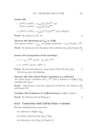
![182 Chapter 6. Cut-elimination stable fragments
By composing the first two connections, we have a Galois connection from λLJQ
to λF
CPS, and together with last one, we have a a pre-Galois connection from
λLJQ to λC. The compositions of these connections also form an equational
correspondence between λLJQ to λC. These facts imply the following theorem:
Theorem 187 (Connections between λLJQ and λC) Let us write V for
(↑ (V F
))
back
, M for (↑ (M :F k))back
, V for (V †
)
Fback
and M for (M : k)Fback
.
1. For any terms M and N of λC, if M −→λCβ
N then M −→∗
λLJQ N .
2. For any terms M and N of λLJQ, if M −→λLJQ N then M −→∗
λCβ
N .
3. For any term M of λC, M←→∗
λCβ
M .
4. For any term M of λLJQ, M−→∗
λLJQ M .
Proof: By composition of the reflections and Galois connection. P
Corollary 188 (Equational correspondence between λLJQ and λC)
1. For any terms M and N of λLJQ, M←→∗
λLJQ N if and only if M ←→∗
λCβ
N .
2. For any terms M and N of λC, M←→∗
λCβ
N if and only if M ←→∗
λLJQ N .
We can give the composition of encodings explicitly. We have for instance the
following theorem:
Theorem 189 (From λC to λLJQ) The following equations hold:
x = x
(λx.M) = λx.M
V = [V ]
(let y = x V in P) = x[V , y.P ]
(let y = (λx.M) V in P) = λx.M † z.z[V , y.P ]
(let z = V N in P) = (let y = N in (let z = V y in P))
if N is not a value
(let z = M N in P) = (let x = M in (let z = x N in P))
if M is not a value
(let z = (let x = M in N) in P) = (let x = M in (let z = N in P))
(let y = V in P) = V † y.P
(M N) = (let y = M N in y)
Proof: By structural induction, unfolding the definition of the encodings on
both sides of each equation. P](https://image.slidesharecdn.com/frenchenglish-150412084606-conversion-gate01/85/French-english-206-320.jpg)
![6.3. Q-restriction LJQ 183
In fact, we could take this set of equalities as the definition of the direct
encoding of λC into λLJQ. For that it suffices to check that there is a measure
that makes this set of equations a well-founded definition. We now give this
measure, given by an encoding of the terms of λC into first-order terms equipped
with an LPO.
Definition 106 (An LPO for λC) We encode λC into the first-order syntax
given by the following term constructors and their precedence relation:
ap(_, _) let(_, _) ii(_, _) i(_)
The precedence relation generates a terminating LPO as presented in Defi-
nition 52. The encoding is given in Fig. 6.20. We can now consider the (termi-
nating) relation induced by through the reverse relation of the encoding as a
measure for λC.
x :=
λx.M := i(M)
let x = M1 M2 in N := let(ii(M1, M2), N)
let x = M in N := let(M, N) otherwise
M N := ap(M, N)
Figure 6.20: Encoding of λC into the first-order syntax
Remark 190 let(M, N)let x = M in N or let(M, N) = let x = M in N.
In the other direction, we have:
Theorem 191 (From λLJQ to λC)
x = x
(λx.M) = λx.M
V †x.V = V
x V
[V ] = V
(x[V, y.M]) = let y = x V in M
N † x.M ∗
λCβ
←− let x = N in M
V †x.M = V
x M
Proof: By structural induction, unfolding the definition of the encodings on
each side and using Lemma 76. Also note that we do not have an equality in the
penultimate line but only a reduction. This prevents the use of this theorem as
a definition for the encoding from λLJQ to λC, although refining this case (with
different sub-cases) could lead to a situation like that of Theorem 189 (with a
measure to find in order for the set of equations to form a well-formed definition).
P](https://image.slidesharecdn.com/frenchenglish-150412084606-conversion-gate01/85/French-english-207-320.jpg)
![184 Chapter 6. Cut-elimination stable fragments
Remark 192 Note from Theorem 189 and Theorem 191 that if M is a cut-free
term of λLJQ, M = M.
The connection between λLJQ and λC suggests to restricts λC by always requir-
ing (a series of) applications to be explicitly given with a contination, i.e. to refuse
a term of λC such as λx.M1 M2 M3 but only accept λx.let y = M1 M2 M3 in y.
The refined Fischer translation from Chapter 3, on that particular fragment of
λC, directly has λf
CPS as its target calculus, and the equational correspondence
between λC d λLJQ would then also become a pre-Galois connection from the
former to the latter. The fragment is not stable under rule ηlet, and corresponds
to the terms of λC in some notion of ηlet-long form.
This restriction can be formalised with the syntax of a calculus given in [Esp05]:
M, N, P ::= x | λx.M | let x = E in M
E ::= M | E M
In fact, this calculus is introduced in [Esp05] as a counterpart, in natural deduc-
tion, of a sequent calculus. Hence, it seems that it is the adequate framework
for formalising in natural deduction the concepts developed in this chapter about
sequent calculus, in particular the CBN- and CBV-reductions, and the t- and
q-restrictions. This calculus would thus capture both the traditional λ-calculus
and (the ηlet-long forms of) λC. Further work includes investigating the relation
between this calculus and λG3.
Conclusion
This chapter surveyed some computational notions in λG3 based on cut-elimination
in the sequent calculus G3ii. It presented various propagation systems with a
comparative approach and a general framework with proof-terms, in which CBV
and CBN sub-systems were generically defined. In each case, confluence of these
sub-systems is only conjectured, which gives a direction for further work.
This chapter then presented the t- and q-restrictions of λG3/G3ii, both in the
proof-terms and in the logic, corresponding to the sequent calculi LJT and LJQ.
The two fragments are respectively stable under CBN- and CBV-reduction.
We recalled the strong connection between the t-fragment and the (CBN)
λ-calculus by means of a reflection in the calculus λ, and derived from this con-
nection some properties of λ such as confluence, PSN and strong normalisation of
typed terms (illustrating the use of the safeness and minimality technique from
Chapter 2).
We established some new results about the q-fragment and the CBV λ-calculus,
expressed via Moggi’s λC-calculus presented in Chapter 3. Further development of
the material in this section about LJQ and λC is ongoing work, including refining
the encodings and the simulations to have a Galois connection or a reflection.](https://image.slidesharecdn.com/frenchenglish-150412084606-conversion-gate01/85/French-english-208-320.jpg)
![Conclusion 185
Once this is done, a promising direction for further work is given by the
calculus from [Esp05] in natural deduction that encompasses both the traditional
(CBN) λ-calculus and (a minor variant of) the CBV λC-calculus, with a very strong
connection with sequent calculus as a whole (i.e. not just with the t-fragment or
the q-fragment).](https://image.slidesharecdn.com/frenchenglish-150412084606-conversion-gate01/85/French-english-209-320.jpg)

![Chapter 7
A higher-order calculus for G4ii
In this chapter, whose contents appeared in [DKL06], we apply the same tech-
nique as in Chapter 6 to the sequent calculus G4ii (as it is called in [TS00]) for
intuitionistic propositional logic.
Independently developed in [Hud89, Hud92] and [Dyc92] (see also [LSS91]),
it has the strong property of being depth-bounded, in that proofs are of bounded
depth and thus (for root-first proof search) no loop-checking is required. This
contrasts with other calculi for this logic such as G3ii, where proofs can be of
unbounded depth. Its essential ingredients appeared already in 1952 work of
Vorob’ev, published in detail in [Vor70].
Its completeness can be shown by various means, either indirectly, using the
completeness of another calculus and a permutation argument [Dyc92], or di-
rectly, such as in [DN00] where cut-admissibility is proved without reference to
the completeness of any other sequent calculus.
As described in Chapter 6, such an admissibility proof can be seen, via the
Curry-Howard correspondence, as a weakly normalising proof-reduction system.
Again we present a formulation of implicational G4ii with derivations represented
by terms; strong (instead of weak) normalisation is proved by the use of a MPO.
Several variations, all of them being strongly normalising, are considered, depend-
ing on whether we want to have a system as general as possible or a system more
restricted (but simpler) implementing some reduction strategy.
The merits of G4ii for proof-search and automated reasoning have been dis-
cussed in many papers (see [ORK05] for some recent pointers; note its use of an
old name LJT for G4ii). However, a question that has been less investigated is
the following: what are the proofs expressed in G4ii and what is their seman-
tics? Here we investigate an operational, rather than denotational, semantics
because it is more directly related to inductive proofs of cut-admissibility (such
as in [DN00]). Further work will investigate denotational semantics, by relating
these proofs and their reductions to the simply-typed λ-calculus.
In contrast to previous work, we present G4ii with a term syntax, and our
approach to cut-elimination differs from that in [DN00], which showed (using
187](https://image.slidesharecdn.com/frenchenglish-150412084606-conversion-gate01/85/French-english-211-320.jpg)
![188 Chapter 7. A higher-order calculus for G4ii
logical sequents) first the admissibility of contraction and then the admissibility
of context-splitting (a.k.a. multiplicative) cut. By rather using a context-sharing
(a.k.a. additive) cut (which is easier to handle with proof-terms since no linearity
constraint restricts the cut-constructor), admissibility of contraction follows as a
special case of that of cut.
To some extent, Matthes [Mat02] also investigated terms and reductions corre-
sponding to cut-elimination in G4ii, with a variety of motivations, such as that of
understanding better Pitts’ algorithm [Pit92] for uniform interpolation. His work
is similar to ours in using terms to represent derivations; but it differs conceptu-
ally from ours by considering not the use of explicit operators for the cut-rule but
the closure of the syntax under (implicit) substitution, as in λ-calculus, where
the general syntax of λ-terms may be regarded as the extension of the normal
λ-terms by such a closure. His reduction rules are global (using implicit substitu-
tions) rather than local (using explicit operators); strong normalisation is shown
for a subset of the reductions, but unfortunately not for all that are required.
The chapter is organised as follows. Section 7.1 describes the steps that change
G3ii into G4ii. Section 7.2 presents the term syntax and typing rules of our HOC for
G4ii and its auxiliary (admissible) rules. Section 7.3 studies proof transformations
and reduction rules of the calculus. Section 7.4 shows a translation from the
derivations of the calculus to a first-order syntax and proves that every reduction
step satisfies subject reduction and decreases first-order terms with respect to an
MPO, thus proving strong normalisation. In Section 7.5 we discuss variants for
the reduction system introduced in Section 7.3, some of them being confluent.
Finally we conclude and give some ideas for further work.
7.1 From G3ii to G4ii
In this section we describe the steps that transform G3ii into G4ii.
Definition 107 (Standard terms of λG3) A term is standard if in any sub-
term of the form y[N, x.M], y ∈ FV(M).
In a typed framework, this corresponds to changing the left-introduction to the
following one:
Γ, x:A→B M :A Γ, y:B N :C
Γ, x:A→B x[M, y.N]:C
We call this sequent calculus G3ii , and the following purification rule standardises
terms, but using cuts:
x[M, y.N] −→purG3ii x[M, y. λz.y † x.N ]
Clearly this rule is non-terminating unless the side-condition y ∈ FV(M) ensures
that the application of the rule is actually needed.](https://image.slidesharecdn.com/frenchenglish-150412084606-conversion-gate01/85/French-english-212-320.jpg)
![7.1. From G3ii to G4ii 189
Unfortunately, G3ii is not stable under either CBN or CBV-reductions, so
eliminating the cut introduced by purG3ii can produce non-standard terms so
that purG3ii is needed again. Hence, it would be interesting to prove that adding
this rule to the reductions of λG3 does not break strong normalisation on typed
terms. Alternatively we could also look for an internal reduction system for G3ii ,
by dropping the side-condition purG3ii but rather integrating the rule to each
rewrite rule that might produce a non-standard term.
Now this rule is interesting in that it is the first rule we introduce that makes
a semantical jump: so far, all the rules reducing terms of λG3 leave the image by
G1
in the same βη-class. This one, on the contrary, jumps from one to another,
as noticed by Vestergaard [Ves99].
f[x, y.f[y, z.z]] −→purG3ii f[x, y. λy .y † f.f[y, z.z] ]−→∗
f[x, z.z]
while G1
(f[x, y.f[y, z.z]]) = f (f x) and
G1
(f[x, y. λy .y † f.f[y, z.z] ]) = G1
(f[x, z.z]) = f x.
More generally for n ≥ 2 we have by induction
f[x, xn. . . . f[x2, x1.x1]] −→∗
i.h. f[x, xn.f[xn, x1.x1]]
−→∗
f[x, x1.x1]
The G4ii-calculus is built from the combination of G3ii with the q-restriction.
Indeed, such a combination replaces rule →left of G3ii by the following ones:
Γ, y: A, z: B N: E
Γ, x: A→B, y: A x[y, z.N]: E
Γ, y: C, x: (C→D)→B M: D Γ, z: B N: E
Γ, x: (C→D)→B x[λy.M, z.N]: E
with x ∈ FV(N) in both cases (the restriction of being standard).
We obtain these two rules only by case analysis on the proof-term of the first
premiss in the left-introduction rule of LJQ: it must be a value, so it is either a
variable y or an abstraction λy.M.
The restriction of G3ii forbids x to appear in N because it can use z instead,
which has a logically stronger type, and this already drastically reduces the set
of proofs (without losing completeness, see e.g. [TS00]).
For instance, all Church numerals (but zero) collapse to 1: Let n be the
Church numeral n in λ-calculus, i.e. λx.λf.f (. . . f x) (with n occurrences of f),
we encode them in the q-fragment. Suppose n ≥ 2.
Pr(n) = G2
(n) = λx.λf.f[. . . f[x, xn.xn], x1.x1]
−→∗
pur-q,CBV λx.λf.f[x, xn. . . . f[x2, x1.x1]]
−→∗
purG3ii ,CBV λx.λf.f[x, x1.x1]
−→∗
Pr(1)](https://image.slidesharecdn.com/frenchenglish-150412084606-conversion-gate01/85/French-english-213-320.jpg)
![190 Chapter 7. A higher-order calculus for G4ii
The G4ii sequent calculus takes the even more drastic step of forbidding x (of
type (C →D)→B) in M but allowing a variable v with a type D →B which,
in presence of C (the type of y) is intuitionistically equivalent to (C →D)→B.
Hence, we get the rule:
Γ, z :C, v:D→B M :B Γ, y:B N :C
Γ, x:(C→D)→B x[z.v.M, y.N]:C
with a new constructor for the rule: x[z.v.M, y.N].
An interpretation of this constructor in λG3 could be:
x[λz. λw.x[λu.w, y .y ] † v.M , y.N]
As we shall see, the move from the q-restriction of G3ii’ to G4ii is what provides
the property of being depth-bounded. As we shall see, logical completeness is not
lost, but there is clearly some computational completeness that is lost (compared
to, say, λG3 or λ-calculus): it was already the case for the q-restriction of G3ii’,
but even more proofs are lost in G4ii. On the other hand, depth-boundedness is
very convenient for proof-search, since they ensure finiteness of search space.
7.2 An HOC for G4ii
7.2.1 Syntax
Definition 108 (Grammar of Terms)
M, N ::= x | λx.M | x[y, z.M] | x[u.v.M, z.N] |
inv(x, y.M) | dec(x, y, z.M) | M † x.N
In this definition, the first line defines the syntax for normal terms (cor-
responding to primitive derivations) and the second gives the extra syntax for
auxiliary terms, which may be built up using also the “auxiliary constructors”
that appear in bold teletype font, such as cut. Six of the eight term constructors
use variable binding: in λx.M, x binds in M; in x[y, z.M], z binds in M; in
x[u.v.M, z.N], u and v bind in M and z binds in N; in inv(x, y.M), y binds in
M; in dec(x, y, z.M), z binds in M; and in M † x.N , x binds in N.
Certain constraints on the use of the term syntax will be evident once we
present the typing rules; these constraints are captured by the notion of well-
formed term, mentioned in Chapter 2 and defined in the case of G4ii as follows:
Definition 109 (Well-formed term) A term L is well-formed if in any sub-
term of the form
• x[y, z.M], we have x = y, with x not free in M;](https://image.slidesharecdn.com/frenchenglish-150412084606-conversion-gate01/85/French-english-214-320.jpg)
![7.2. An HOC for G4ii 191
• x[u.v.M, z.N], we have u = v, with x not free in M and not free in N;
• inv(x, y.M), we have x not free in M;
• dec(x, y, z.M), we have x = y, with both of them not free in M.
Definition 110 (Ordering on multi-sets of types) We compare multi-sets of
types with the traditional multi-set ordering, denoted mul, while types are com-
pared according to their sizes (as trees).
For every rule of the logical sequent calculus G4ii, the multi-set of types ap-
pearing in the conclusion is greater than that of each premiss. Hence, we say
that G4ii is depth-bounded. See [Dyc92] or [TS00] for details, and see the next
section for the corresponding property in our version of G4ii with terms.
7.2.2 Typing
The next definition adds term notation to the rules for implication of G4ii; another
view is that it shows how the untyped normal terms of the above grammar may
be typed.
Definition 111 (Typing Rules for Normal Terms)
Ax
Γ, x: A x: A
Γ, x: A M: B
R→
Γ λx.M: A→B
Γ, y: A, z: B M: E
L0→
Γ, x: A→B, y: A x[y, z.M]: E
Γ, u: C, v: D→B M: D Γ, z: B N: E
L→→
Γ, x: (C→D)→B x[u.v.M, z.N]: E
These rules only construct well-formed terms; e.g. the notation Γ, x: A→B, y: A
in the conclusion of L0 → forces x = y and x to be not already declared in Γ
(hence not free in M).
These rules are the extensions with terms of the logical rules of G4ii in [TS00]
(note a slight difference of the L→→rule from that of [Dyc92]), with the variation
that both in Ax and in L0→the type A need not be atomic. In the rules R→,
L0→and L→→the types A→B, A→B and (C→D)→B respectively are principal;
in L0 → the type A is auxiliary. (This use of “auxiliary” is not to be confused
with its use in Definition 108 to describe certain kinds of term.)
Remark 193 Note that, in both cases, terms reflect the structure of their typing
derivation: for each derivable sequent Γ M: A there is a unique derivation tree](https://image.slidesharecdn.com/frenchenglish-150412084606-conversion-gate01/85/French-english-215-320.jpg)
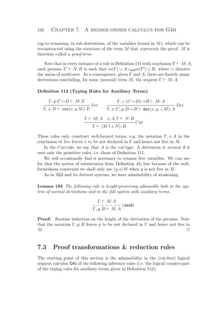
![7.3. Proof transformations reduction rules 193
Γ, C→D E
Inv
Γ, D E
Γ, (C→D)→B A
Dec
Γ, C, D→B A
Γ A A, Γ B
Cut
Γ B
The admissibility in G4ii of Inv alone can be proved by induction on the
height of the derivation of the premiss. For the admissibility of Dec and Cut we
can use a simultaneous induction, the admissibility of one rule being recursively
used for the admissibility of the other. The measure now uses the multi-set of
types appearing in the unique premiss for Dec and in the second premiss for Cut.
In other words, the induction can be done on {{Γ, (C→D)→B, A}} for Dec and
on {{Γ, A, B}} for Cut.
We do not include here the detail of these proofs of admissibility, because the
property turns out to be a consequence (Corollary 199) of our strong normalisa-
tion result for our calculus with terms.
Indeed, the admissibility property means, in our framework with terms, that
a term M with auxiliary constructors inv, dec or cut can be transformed into
another term M with the same type in the same context that does not use
these constructors. In other words, it means that the auxiliary typing rules are
term-irrelevant admissible in the system of normal derivations. As described in
Chapter 6 we extract from these proofs a rewrite system, such that the measures
for induction mentioned above can be used (as part of a MPO —see section 7.4)
to conclude their strong normalisation as well. We give in Fig. 7.1 and Fig. 7.2
the reduction systems that eliminate the auxiliary constructors inv and dec. All
these rules, which we call system ivdc, will be part of the different variants that
we are going to introduce.
inv(x, y.z) −→i1 z
inv(x, y.y) −→i2 λz.x
inv(x, y.λz.M) −→i3 λz.inv(x, y.M)
inv(x, y.y[w, z.N]) −→i4 (x z)N
inv(x, y.y[u.v.M, z.N]) −→i5 (x z)N
inv(x, y.w[y, z.N]) −→i6 w[u.v.x, z.inv(x, y.N)]
inv(x, y.y [w, z.N]) −→i7 y [w, z.inv(x, y.N)]
inv(x, y.y [u.v.M, z.N]) −→i8 y [u.v.inv(x, y.M), z.inv(x, y.N)]
Figure 7.1: Reduction rules for inv-terms
The structure cut-reduction system follows the general pattern of cut-reduction
systems described in Chapter 6: the rules can be split into three kinds
(Kind1, Kind2, Kind3), according to whether they push cuts to the right, to the
left, or they reduce logical cuts, breaking them into cuts on smaller types.
Here, owing to the particular inference rules of G4ii and the well-formedness](https://image.slidesharecdn.com/frenchenglish-150412084606-conversion-gate01/85/French-english-217-320.jpg)
![194 Chapter 7. A higher-order calculus for G4ii
dec(x, y, z.w) −→d1 w
dec(x, y, z.z) −→d2 λv.v[x, w.y[w, u.u]]
dec(x, y, z.λw.M) −→d3 λw.dec(x, y, z.M)
dec(x, y, z.w[u.v.M, w .N]) −→d4 w[u.v.dec(x, y, z.M), w .dec(x, y, z.N)]
dec(x, y, z.w[y , z .M]) −→d5 w[y , z .dec(x, y, z.M)]
dec(x, y, z.z[y , z .M]) −→d6 y [x, z .y[z , z .inv(z , y .M)]]
dec(x, y, z.x [z, z .M]) −→d7 x[u.v.v[x, z .y[z , w.w]], z .dec(x, y, z.M)]
dec(x, y, z.z[u.v.M, z .N]) −→d8 (x u)(y v)M † y .y[y , z .N]
Figure 7.2: Reduction rules for dec-terms
Kind1
M † x.x −→c1 M
M † x.y −→c2 y
M † x.λy.N −→c3 λy. M † x.N
M † x.y[z, w.N] −→c4 y[z, w. inv(w, y.M) † x.N ]
M † x.y[u.v.N , w.N] −→c5 y[u.v.P, w. inv(w, y.M) † x.N ]
where P = dec(u, v, y.M) † x.N
λz.M † x.y[x, w.N] −→c6 y[u.v.P, w. inv(w, y.λz.M) † x.N ]
where P = u † z.dec(u, v, y.M)
z † x.y[x, w.N] −→c7 y[z, w. z † x.N ]
Kind2
y[z, w.M] † x.N −→c8 y[z, w. M † x.inv(w, y.N) ]
y[u.v.M , w.M] † x.N −→c9 y[u.v.M , w. M † x.inv(w, y.N) ]
Figure 7.3: Cut-elimination rules cers/cears (Kind1 and Kind2)
Kind3
λy.M † x.x[z, w.N] −→C z † y.M † w.N
λy.M † x.x[u.v.N , w.N] −→D λu. λz.inv(z, y.M) † v.N † y.M † w.N
y † x.x[z, w.N] −→E y[z, w . w † w.inv(w , y.N) ]
y † x.x[u.v.N , w.N] −→F y[u .v . u † u.P , w . w † w.inv(w , y.N) ]
where P := dec(u , v , y. λy .y[u.v.y , z.z] † v.N )
Figure 7.4: Cut-elimination rules cers (Kind3)](https://image.slidesharecdn.com/frenchenglish-150412084606-conversion-gate01/85/French-english-218-320.jpg)
![7.4. Subject reduction strong normalisation 195
Kind3
λy.M † x.x[z, w.N] −→C z † y.M † w.N
λy.M † x.x[u.v.N , w.N] −→D λu. λz.inv(z, y.M) † v.N † y.M † w.N
y † x.x[z, w.N] −→E y[z, w . w † w.inv(w , y.N) ]
y † x.x[u.v.N , w.N] −→G y[u .v . u † u.P , w . w † w.inv(w , y.N) ]
where P := v † v.dec(u , v , y.N )
Figure 7.5: Cut-elimination rules cears (Kind3)
constraints they impose on terms, the rewrite rules must use the auxiliary con-
structs inv and dec, rather than just propagate the cuts.
For the third kind of cut-reduction rules, reducing logical cuts, we have an
alternative between rule −→F by −→G , discussed in section 7.5, and leading to
two different systems called rs (with −→F ) or ars (with −→G ).
Summing up :
Name of the System Reduction Rules
ivdc Fig. 7.1 and Fig. 7.2
cers/cears Fig. 7.3, and Fig. 7.4/7.5
rs/ars ivdc ∪ cers/ivdc ∪ cears
Lemma 195 All rules of system rs and ars are such that well-formed terms reduce
to well-formed terms.
Proof: Routine. P
7.4 Subject reduction strong normalisation
In this section we prove two fundamental properties of systems rs and ars. The
first one is subject reduction and it guarantees that types are preserved by the
reduction system. The second one is strong normalisation on typed terms of
the rewrite systems of section 7.3, which guarantees that no infinite reduction
sequence starts from a typed term.
The latter is proved using a simulation by MPO-reduction in a first-order
syntax that encodes typing derivations. It is convenient to prove the simulation
together with subject reduction since the proofs are based on the same case
analysis.](https://image.slidesharecdn.com/frenchenglish-150412084606-conversion-gate01/85/French-english-219-320.jpg)
![196 Chapter 7. A higher-order calculus for G4ii
The first-order syntax is given by the following infinite signature and its prece-
dence relation:
Cn
(_, _) Dn
(_) · · · Cm
(_, _) Dm
(_) J(_) K(_, _) I(_)
for all multi-sets of types nmulm.
The precedence relation on symbols provides an MPO on first-order terms.
Remark 196
1. The order on types (Definition 110) is terminating, so mul is terminat-
ing [DM79].
2. The order mul is terminating, so is also terminating.
3. The order is terminating, so the MPO is also terminating (Theo-
rem 49).
Definition 113 (Encoding into the first-order syntax) Derivations are
mapped to the first-order syntax according to Fig. 7.6. Note that since each
sequent Γ M: A has at most one derivation, we write φ(Γ M: A) for such a
translation, and even φ(M) when the environment and the type are clear from
context.
φ(Γ, x: A x: A) :=
φ(Γ λx.M: A→B) := I(φ(M))
φ(Γ, x: A→B, y: A x[y, z.M]: E) := I(φ(M))
φ(Γ, x: (C→D)→B x[u.v.M, z.N]: E) := K(φ(M), φ(N))
φ(Γ, x: D inv(x, y.M): E) := J(φ(M))
φ(Γ, x: C, y: D→B dec(x, y, z.M): A) := Dk
(φ(Γ, z: (C→D)→B M: A))
where k := {{Γ, (C→D)→B, A}}
φ(Γ M † x.N : B) := Ck
(φ(Γ M: A), φ(x: A, Γ N: B))
where k := {{Γ, A, B}}
Figure 7.6: Encoding into the first-order syntax
Observe that φ(M) = φ((x y)M) for any renaming of M.
Theorem 197 If Γ L: E and L −→rs,ars L , then Γ L : E and φ(L)φ(L ).
Proof: By induction on the derivation of Γ L: E. We show only the cases
of root-reduction.
i1 inv(x, y.z) −→i1 z](https://image.slidesharecdn.com/frenchenglish-150412084606-conversion-gate01/85/French-english-220-320.jpg)
![7.4. Subject reduction strong normalisation 197
The derivation
Ax
Γ , z: E, y: A→B z: E
Inv
Γ , z: E, x: B inv(x, y.z): E
rewrites to
Ax
Γ , z: E, x: B z: E
Also, φ(L) = J( ) = φ(L ) holds by the sub-term property of .
i2 inv(x, y.y) −→i2 λz.x
The derivation
Ax
Γ , y: A→B y: A→B
Inv
Γ , x: B inv(x, y.y): A→B
rewrites to
Ax
Γ , x: B, z: A x: B
R→
Γ , x: B λz.x: A→B
Also, φ(L) = J( ) I( ) = φ(L ) holds by J I.
i3 inv(x, y.λz.M) −→i3 λz.inv(x, y.M) with E = C→D
The derivation
Γ , y: A→B, z: C M: D
R→
Γ , y: A→B λz.M: C→D
Inv
Γ , x: B inv(x, y.λz.M): C→D
rewrites to
Γ , y: A→B, z: C M: D
Inv
Γ , x: B, z: C inv(x, y.M): D
R→
Γ , x: B λz.inv(x, y.M): C→D
Also, φ(L) = J(I(φ(M)))I(J(φ(M))) = φ(L ) by J I.
i4 inv(x, y.y[w, z.N]) −→i4 (x z)N
The derivation
Γ , w: A, z: B N: E
L0→
Γ , w: A, y: A→B y[w, z.N]: E
Inv
Γ , w: A, x: B inv(x, y.y[w, z.N]): E](https://image.slidesharecdn.com/frenchenglish-150412084606-conversion-gate01/85/French-english-221-320.jpg)
![198 Chapter 7. A higher-order calculus for G4ii
rewrites to
Γ , w: A, z: B N: E
− − − − − − − − − − − −
Γ , w: A, x: B (x z)N: E
by equivariance of typing systems.
Also, φ(M) = J(I(φ(N)))φ(N) = φ(M ) holds by the sub-term property
of .
i5 inv(x, y.y[u.v.M, z.N]) −→i5 (x z)N with A = C→D
The derivation
Γ , u: C, v: D→B M: D Γ , z: B N: E
L→→
Γ , y: A→B y[u.v.M, z.N]: E
Inv
Γ , x: B inv(x, y.y[u.v.M, z.N]): E
rewrites to
Γ , z: B N: E
− − − − − − − − −
Γ , x: B (x z)N: E
by equivariance of typing systems.
Also, φ(L) = J(K(φ(M), φ(N)))φ(N) = φ(L ) holds by the sub-term
property of .
i6 inv(x, y.w[y, z.N]) −→i6 w[u.v.x, z.inv(x, y.N)]
The derivation
Γ , y: A→B, z: C N: E
L0→
Γ , w: (A→B)→C, y: A→B w[y, z.N]: E
Inv
Γ , w: (A→B)→C, x: B inv(x, y.w[y, z.N]): E
rewrites to
Ax
Γ , x: B, u: A, v: B→C x: B
Γ , y: A→B, z: C N: E
Inv
Γ , x: B, z: C inv(x, y.N): E
L→→
Γ , w: (A→B)→C, x: B w[u.v.x, z.inv(x, y.N)]: E
Also, φ(L) = J(I(φ(N)))K( , J(φ(N))) = φ(L ) by J K, .
i7 inv(x, y.y [w, z.N]) −→i7 y [w, z.inv(x, y.N)]
The derivation
Γ , w: C, z: D, y: A→B N: E
L0→
Γ , w: C, y : C→D, y: A→B y [w, z.N]: E
Inv
Γ , w: C, y : C→D, x: B inv(x, y.y [w, z.N]): E](https://image.slidesharecdn.com/frenchenglish-150412084606-conversion-gate01/85/French-english-222-320.jpg)
![7.4. Subject reduction strong normalisation 199
rewrites to
Γ , w: C, z: D, y: A→B N: E
Inv
Γ , w: C, z: D, x: B inv(x, y.N): E
L0→
Γ , w: C, y : C→D, x: B y [w, z.inv(x, y.N)]: E
Also, φ(L) = J(I(φ(N)))I(J(φ(N))) = φ(L ) by J I.
i8 inv(x, y.y [u.v.M, z.N]) −→i8 y [u.v.inv(x, y.M), z.inv(x, y.N)]
The derivation
Γ , y: A→B, u: C, v: D→B M: D Γ , y: A→B, z: B N: E
L→→
Γ , y : (C→D)→B , y: A→B y [u.v.M, z.N]: E
Inv
Γ , y : (C→D)→B , x: B inv(x, y.y [u.v.M, z.N]): E
rewrites to
Γ , y: A→B, u: C, v: D→B M: D
Inv
Γ , x: B, u: C, v: D→B inv(x, y.M): D
Γ , y: A→B, z: B N: E
Inv
Γ , x: B, z: B inv(x, y.N): E
L→→
Γ , y : (C→D)→B , x: B y [u.v.inv(x, y.M), z.inv(x, y.N)]: E
Also, φ(L) = J(K(φ(M), φ(N)))K(J(φ(M)), J(φ(N))) = φ(L ) by J K.
d1 dec(x, y, z.w) −→d1 w
The derivation
Ax
Γ , w: E, z: (C→D)→B w: E
Dec
Γ , w: E, x: C, y: D→B dec(x, y, z.w): E
rewrites to
Ax
Γ , w: E, x: C, y: D→B w: E
Also, φ(L) = Dm
( ) = φ(L ), where m := {{Γ , E, (C→D)→B, E}}.
d2 dec(x, y, z.z) −→d2 λv.v[x, w.y[w, u.u]].
The derivation
Ax
Γ , z: (C→D)→B z: (C→D)→B
Dec
Γ , x: C, y: D→B dec(x, y, z.z): E](https://image.slidesharecdn.com/frenchenglish-150412084606-conversion-gate01/85/French-english-223-320.jpg)
![200 Chapter 7. A higher-order calculus for G4ii
rewrites to
Ax
Γ , x: C, w: D, u: B u: B
L0→
Γ , x: C, w: D, y: D→B y[w, u.u]: B
L0→
Γ , x: C, y: D→B, v: C→D v[x, w.y[w, u.u]]: B
R→
Γ , x: C, y: D→B λv.v[x, w.y[w, u.u]]: (C→D)→B
Also, φ(L) = Dm
( )I(I(I( ))) = φ(L ),
where m := {{Γ , (C→D)→B, (C→D)→B}}, by Dm
I.
d3 dec(x, y, z.λw.M) −→d3 λw.dec(x, y, z.M).
The derivation
Γ , z: (C→D)→B, w: E1 M: E2
R→
Γ , z: (C→D)→B λw.M: E1→E2
Dec
Γ , x: C, y: D→B dec(x, y, z.λw.M): E1→E2
rewrites to
Γ , z: (C→D)→B, w: E1 M: E2
Dec
Γ , x: C, y: D→B, w: E1 dec(x, y, z.M): E2
R→
Γ , x: C, y: D→B λw.dec(x, y, z.M): E1→E2
Let m := {{Γ , (C→D)→B, E1→E2}} and n := {{Γ , (C→D)→B, E1, E2}}.
We have
φ(L) = Dm
(I(φ(M)))I(Dn
(φ(M))) = φ(L )
since Dm
I, Dn
because mmuln.
d4 dec(x, y, z.w[u.v.M, w .N]) −→d4 w[u.v.dec(x, y, z.M), w .dec(x, y, z.N)].
The derivation
Γ , v: F, u: G→H, z: (C→D)→B M: G Γ , w : H, z: (C→D)→B N: E
L→→
Γ , w: (F→G)→H, z: (C→D)→B w[u.v.M, w .N]: E
Dec
Γ , w: (F→G)→H, x: C, y: D→B dec(x, y, z.w[u.v.M, w .N]): E
rewrites to
Γ , v: F, u: G→H, z: (C→D)→B M: G
Dec
Γ , v: F, u: G→H, x: C, y: D→B M : G
Γ , w : H, z: (C→D)→B N: E
Dec
Γ , w : H, x: C, y: D→B N : E
L→→
Γ , w: (F→G)→H, x: C, y: D→B w[u.v.M , w .N ]: G
with M := dec(x, y, z.M) and N := dec(x, y, z.N).](https://image.slidesharecdn.com/frenchenglish-150412084606-conversion-gate01/85/French-english-224-320.jpg)
![7.4. Subject reduction strong normalisation 201
Let k := {{Γ , (F →G)→H, (C→D)→B, E}} and
m := {{Γ , F, G→H, (C→D)→B, G}} and n := {{Γ , H, (C→D)→B, E}}.
We have
φ(L) = Dk
(K(φ(M), φ(N)))K(Dm
(φ(M), Dn
(φ(N))) = φ(L )
since Dk
K, Dm
, Dn
because kmulm, n.
d5 dec(x, y, z.w[y , z .M]) −→d5 w[y , z .dec(x, y, z.M)].
The derivation
Γ , y : F, z : G, z: (C→D)→B M: E
L0→
Γ , y : F, w: F→G, z: (C→D)→B w[y , z .M]: E
Dec
Γ , y : F, w: F→G, x: C, y: D→B dec(x, y, z.w[y , z .M]): E
rewrites to
Γ , y : F, z : G, z: (C→D)→B M: E
Dec
Γ , y : F, z : G, x: C, y: D→B dec(x, y, z.M): E
L0→
Γ , y : F, w: F→G, x: C, y: D→B w[y , z .dec(x, y, z.M)]: E
Let k := {{Γ , F, F →G, (C→D)→B, E}} and
m := {{Γ , F, G, (C→D)→B, E}}. We have
φ(L) = Dk
(I(φ(M)))I(Dm
(φ(M))) = φ(L )
since Dk
I, Dm
because kmulm.
d6 dec(x, y, z.z[y , z .M]) −→d6 y [x, z .y[z , z .inv(z , y .M)]].
The derivation
Γ , y : C→D, z : B M: E
L0→
Γ , z: (C→D)→B, y : C→D z[y , z .M]: E
Dec
Γ , x: C, y: D→B, y : C→D dec(x, y, z.z[y , z .M]): E
rewrites to
Γ , y : C→D, z : B M: E
Inv
Γ , z : D, z : B inv(z , y .M): E
L0→
Γ , z : D, y: D→B y[z , z .inv(z , y .M)]: E
− − − − − − − − − − − − − − − − − − − − − − − weak
Γ , x: C, z : D, y: D→B y[z , z .inv(z , y .M)]: E
L0→
Γ , y : C→D, x: C, y: D→B y [x, z .y[z , z .inv(z , y .M)]]: E
Also, φ(L) = Dk
(I(φ(M)))I(I(J(φ(M)))) = φ(L ) since Dk
I, J, where
k := {{Γ , (C→D)→B, C→D, E}}.](https://image.slidesharecdn.com/frenchenglish-150412084606-conversion-gate01/85/French-english-225-320.jpg)
![202 Chapter 7. A higher-order calculus for G4ii
d7 dec(x, y, z.x [z, z .M]) −→d7 x[u.v.v[x, z .y[z , w.w]], z .dec(x, y, z.M)].
The derivation
Γ , z: (C→D)→B, z : A M: E
L0→
Γ , x : ((C→D)→B)→A, z: (C→D)→B x [z, z .M]: E
Dec
Γ , x : ((C→D)→B)→A, x: C, y: D→B dec(x, y, z.x [z, z .M]): E
rewrites to
D
Γ v[x, z .y[z , w.w]]: B
Γ , z: (C→D)→B, z : A M: E
Dec
Γ , x: C, y: D→B, z : A dec(x, y, z.M): E
L→→
Γ , x: ((C→D)→B)→A, y: C, z: D→B x[u.v.v[x, z .y[z , w.w]], z .dec(x, y, z.M)]: E
where Γ := Γ , x: C, y: D→B, u: B→A, v: C→D and D is the following
derivation:
Ax
Γ , x: C, w: B, u: B→A, z : D w: B
L0→
Γ , x: C, y: D→B, u: B→A, z : D y[z , w.w]: B
L0→
Γ , x: C, y: D→B, u: B→A, v: C→D v[x, z .y[z , w.w]]: B
Let k := {{Γ , (C→D)→B, ((C→D)→B)→A, E}} and
m := {{Γ , (C→D)→B, A, E}}. We have
φ(L) = Dk
(I(φ(M)))K(I(I( )), Dm
(φ(M))) = φ(L )
since Dk
K, I, , Dm
because kmulm.
d8 dec(x, y, z.z[u.v.M, z .N]) −→d8 (y u)(x v)M † y .y[y , z .N] .
The derivation
Γ , v: C, u: D→B M: D Γ , z : B N: E
L→→
Γ , z: (C→D)→B z[u.v.M, z .N]: E
Dec
Γ , x: C, y: D→B dec(x, y, z.z[u.v.M, z .N]): E
rewrites to
Γ , v: C, u: D→B M: D
− − − − − − − − − − − − − − − −
Γ , x: C, y: D→B (y u)(x v)M: D
Γ , z : B N: E
− − − − − − − − − − − − weak
y : D, Γ , x: C, z : B N: E
L0→
y : D, Γ , x: C, y: D→B y[y , z .N]: E
Cut
Γ , x: C, y: D→B (y u)(x v)M † y .y[y , z .N] : E
Let k := {{Γ , (C→D)→B, E}} and j := {{Γ , D, C, D→B, E}}. We have
φ(L) = Dk
(K(φ(M), φ(N)))Cj
(φ(M), I(φ(N))) = φ(L )
since Dk
Cj
, I because kmulj.](https://image.slidesharecdn.com/frenchenglish-150412084606-conversion-gate01/85/French-english-226-320.jpg)
![204 Chapter 7. A higher-order calculus for G4ii
c4 M † x.z[y, w.N] −→c4 z[y, w. inv(w, z.M) † x.N ].
The derivation
Γ , y: C, z: C→B M: A
x: A, Γ , y: C, w: B N: E
L0→
x: A, Γ , y: C, z: C→B z[y, w.N]: E
Cut
Γ , y: C, z: C→B M † x.z[y, w.N] : E
rewrites to
Γ , y: C, z: C→B M: A
Inv
Γ , y: C, w: B inv(w, z.M): A x: A, Γ , y: C, w: B N: E
Cut
Γ , y: C, w: B inv(w, z.M) † x.N : E
L0→
Γ , y: C, z: C→B z[y, w. inv(w, z.M) † x.N ]: E
Let k := {{A, Γ , C, C→B, E}} and j := {{A, Γ , C, B, E}}. We have
φ(L) = Ck
(φ(M), I(φ(N)))I(Cj
(J(φ(M)), φ(N)) = φ(L )
since Ck
I, Cj
, J because kmulj.
c5 M † x.y[u.v.N, z.N ]
−→c5 y[u.v. dec(v, u, y.M) † x.N , z. inv(z, y.M) † x.N ].
The derivation
Γ , y: (C→D)→B M: A
x: A, Γ , v: C, u: D→B N: D x: A, Γ , z: B N : E
L→→
x: A, Γ , y: (C→D)→B y[u.v.N, z.N ]: E
Cut
Γ , y: (C→D)→B M † x.y[u.v.N, z.N ] : E
rewrites to
D
Γ , v: C, u: D→B dec(v, u, y.M) † x.N : D
D
Γ , z: B inv(z, y.M) † x.N : E
L→→
Γ , y: (C→D)→B y[u.v. dec(v, u, y.M) † x.N , z. inv(z, y.M) † x.N ]: E
where D is the following derivation:
Γ , y: (C→D)→B M: A
Dec
Γ , v: C, u: D→B dec(v, u, y.M): A x: A, Γ , v: C, u: D→B N: D
Cut
Γ , v: C, u: D→B dec(v, u, y.M) † x.N : D
and D is the following derivation:
Γ , y: (C→D)→B M: A
Inv
Γ , z: B inv(z, y.M): A x: A, Γ , z: B N : E
Cut
Γ , z: B inv(z, y.M) † x.N : E](https://image.slidesharecdn.com/frenchenglish-150412084606-conversion-gate01/85/French-english-228-320.jpg)
![7.4. Subject reduction strong normalisation 205
Let k := {{A, Γ , (C → D) → B, E}} and j := {{A, Γ , C, D → B, D}} and
i := {{A, Γ , B, E}} and h := {{Γ , (C→D)→B, A}}. We have
φ(L) = Ck
(φ(M), K(φ(N ), φ(N)))
K(Cj
(Dh
(φ(M)), φ(N )), Ci
(J(φ(M)), φ(N)) = φ(L )
since Ck
K, J, Cj
, Ci
, Dh
because kmulj, h, i.
c6 λz.M † x.y[x, w.N]
−→c6 y[u.v. u † w.dec(w, v, y.M) , w. inv(w, y.λz.M) † x.N ].
The derivation
z: C, Γ , y: (C→D)→B M: D
R→
Γ , y: (C→D)→B λz.M: C→D
x: C→D, Γ , w: B N: E
L0→
x: C→D, Γ , y: (C→D)→B y[x, w.N]: E
Cut
Γ , y: (C→D)→B λz.M † x.y[x, w.N] : E
rewrites to
D
Γ , u: C, v: D→B M : D
D
Γ , w: B N : E
L→→
Γ , y: (C→D)→B y[u.v.M , w.N ]: E
where M := u † w.dec(w, v, y.M) , N := inv(w, y.λz.M) † x.N , D is
the following derivation:
Ax
Γ , u: C, v: D→B u: C
u: C, Γ , y: (C→D)→B M: D
Dec
Γ , u: C, w: C, v: D→B dec(w, v, y.M): D
Cut
Γ , u: C, v: D→B u † w.dec(w, v, y.M) : D
and D is the following derivation:
Γ , y: A→B λz.M: C→D
Inv
Γ , w: B inv(w, y.λz.M): C→D x: C→D, Γ , w: B N: E
Cut
Γ , w: B inv(w, y.λz.M) † x.N : E
Let k := {{C→D, Γ , (C→D)→B, E}} and j := {{Γ , C, C, D→B, D}} and
h := {{C, Γ , (C→D)→B, D}} and i := {{C→D, Γ , B, E}}. We have
φ(L) = Ck
(I(φ(M)), I(φ(N)))
K(Cj
( , Dh
(φ(M))), Ci
(J(I(φ(M))), φ(N))) = φ(L )
since Ck
K, , J, I, Cj
, Ci
, Dh
because kmulj, i, h.](https://image.slidesharecdn.com/frenchenglish-150412084606-conversion-gate01/85/French-english-229-320.jpg)
![206 Chapter 7. A higher-order calculus for G4ii
c7 x † y.z[y, w.M] −→c7 z[y, w. x † y.M ].
The derivation
Ax
Γ , x: A, z: A→B x: A
x: A, y: A, w: B, Γ M: E
L0→
x: A, y: A, z: A→B, Γ z[y, w.M]: E
Cut
Γ , x: A, z: A→B x † y.z[y, w.M] : E
rewrites to
Ax
Γ , x: A, w: B x: A x: A, y: A, w: B, Γ M: E
Cut
Γ , x: A, w: B x † y.M : E
L0→
Γ , x: A, z: A→B z[y, w. x † y.M ]: E
Let k := {{A, A, A→B, Γ , E}} and j := {{A, A, B, Γ , E}}. We have
φ(L) = Ck
( , I(φ(M)))I(Cj
( , φ(M))) = φ(L )
since Ck
I, Cj
because kmulj.
c8 z[y, w.M] † x.N −→c8 z[y, w. M † x.inv(w, z.N) ].
The derivation
Γ , y: C, w: B M: A
L0→
Γ , y: C, z: C→B z[y, w.M]: A x: A, Γ , y: C, z: C→B N: E
Cut
Γ , y: C, z: C→B z[y, w.M] † x.N : E
rewrites to
Γ , y: C, w: B M: A
x: A, Γ , y: C, z: C→B N: E
Inv
x: A, Γ , y: C, w: B inv(w, z.N): E
Cut
Γ , y: C, w: B M † x.inv(w, z.N) : E
L0→
Γ , y: C, z: C→B z[y, w. M † x.inv(w, z.N) ]: E
Let k := {{A, Γ , C, C→B, E}} and j := {{A, Γ , C, B, E}}. We have
φ(L) = Ck
(I(φ(M)), φ(N))I(Cj
(φ(M), J(φ(N))) = φ(L )
since Ck
I, Cj
, J because kmulj.
c9 y[u.v.M, z.M ] † x.N −→c9 y[u.v.M, z. M † x.inv(z, y.N) ].
The derivation](https://image.slidesharecdn.com/frenchenglish-150412084606-conversion-gate01/85/French-english-230-320.jpg)
![7.4. Subject reduction strong normalisation 207
Γ , v: C, u: D→B M: D Γ , z: B M : A
L→→
Γ , y: (C→D)→B y[u.v.M, z.M ]: A x: A, Γ , y: (C→D)→B N: E
Cut
Γ , y: (C→D)→B y[u.v.M, z.M ] † x.N : E
rewrites to
Γ , v: C, u: D→B M: D
Γ , z: B M : A
x: A, Γ , y: (C→D)→B N: E
Inv
x: A, Γ , z: B inv(z, y.N): E
Cut
Γ , z: B M † x.inv(z, y.N) : E
L→→
Γ , y: (C→D)→B y[u.v.M, z. M † x.inv(z, y.N) ]: E
Let k := {{A, Γ , (C→D)→B, E}} and j := {{A, Γ , B, E}}. We have
φ(L) = Ck
(K(φ(M), φ(M )), φ(N))
K(φ(M), Cj
(φ(M ), J(φ(N)))) = φ(L )
since Ck
K, Cj
, J because kmulj.
A λy.M † x.x[z, w.N] −→A z † y.M † w.N .
The derivation
Γ , z: C, y: C M: B
R→
Γ , z: C λy.M: C→B
Γ , z: C, w: B N: E
L0→
Γ , z: C, x: C→B x[z, w.N]: E
Cut
Γ , z: C λy.M † x.x[z, w.N] : E
rewrites to
Ax
Γ , z: C z: C Γ , z: C, y: C M: B
Cut
Γ , z: C z † y.M : B Γ , z: C, w: B N: E
Cut
Γ , z: C z † y.M † w.N : E
Let k := {{Γ , C, C→B, E}} and j := {{Γ , C, B, E}} and i := {{Γ , C, C, B}}.
We have
φ(L) = Ck
(I(φ(M)), I(φ(N)))Cj
(Ci
( , φ(M)), φ(N)) = φ(L )
since Ck
, J, Cj
, Ci
because kmulj, i.
B λy.M † x.x[u.v.N, z.N ] −→B λu. λy .inv(y , y.M) † v.N † y.M † z.N .](https://image.slidesharecdn.com/frenchenglish-150412084606-conversion-gate01/85/French-english-231-320.jpg)
![208 Chapter 7. A higher-order calculus for G4ii
The derivation
Γ, y: C→D M: B
Γ λy.M: (C→D)→B
u: C, v: D→B, Γ N: D z: B, Γ N : E
L→→
x: (C→D)→B, Γ x[u.v.N, z.N ]: E
Cut
Γ λy.M † x.x[u.v.N, z.N ] : E
rewrites to
D
Γ M : C→D Γ, y: C→D M: B
Cut
Γ M † y.M : B z: B, Γ N : E
Cut
Γ M † y.M † z.N : E
where M = λu. λy .inv(y , y.M) † v.N and D is the following derivation:
Γ, y: C→D M: B
− − − − − − − − − − − (weak)
Γ, u: C, y: C→D M: B
Inv
Γ, u: C, y : D inv(y , y.M): B
R→
Γ, u: C λy .inv(y , y.M): D→B u: C, v: D→B, Γ N: D
Cut
Γ, u: C λy .inv(y , y.M) † v.N : D
R→
Γ λu. λy .inv(y , y.M) † v.N : C→D
Let k := {{(C→D)→B, Γ, E}} and j := {{B, Γ, E}} and
i := {{Γ, C→D, B}} and h := {{C, D→B, Γ, D}}. We have
φ(L) = Ck
(I(φ(M)), K(φ(N), φ(N )))
Cj
(Ci
(I(Ch
(I(J(φ(M))), φ(N))), φ(M)), φ(N )) = φ(L )
since Ck
I, J, Cj
, Ci
, Ch
because kmulj, i, h.
E y † x.x[z, w.N] −→E y[z, w . w † w.inv(w , y.N) ].
The derivation
Ax
Γ , z: C, y: C→B y: C→B
Γ , z: C, y: C→B, w: B N: E
L0→
Γ , z: C, y: C→B, x: C→B x[z, w.N]: E
Cut
Γ , z: C, y: C→B y † x.x[z, w.N] : E
rewrites to
Ax
Γ , z: C, w : B w : B
Γ , z: C, y: C→B, w: B N: E
Inv
Γ , z: C, w : B, w: B inv(w , y.N): E
Cut
Γ , z: C, w : B w † w.inv(w , y.N) : E
L0→
Γ , z: C, y: C→B y[z, w . w † w.inv(w , y.N) ]: E](https://image.slidesharecdn.com/frenchenglish-150412084606-conversion-gate01/85/French-english-232-320.jpg)
![7.4. Subject reduction strong normalisation 209
Let k := {{Γ , C, C→B, C→B, E}} and j := {{Γ , C, B, B, E}}. We have
φ(L) = Ck
( , I(φ(N)))I(Cj
( , J(φ(N)))) = φ(L )
since Ck
, J, Cj
because kmulj.
F G y † x.x[u.v.N , w.N]
−→F/G y[u .v . u † u.P , w . w † w.inv(w , y.N) ]
with P = dec(u , v , y. λy .y[u .v .y , z.z] † v.N ) for F
and P = v † v.dec(u , v , y.N ) for G.
Γ is of the form Γ , y: (C→D)→B. The derivation
Γ y: (C→D)→B
Γ, u: C, v: D→B N : D Γ, w: B N: E
L→→
Γ, x: (C→D)→B x[u.v.N , w.N]: E
Cut
Γ y † x.x[u.v.N , w.N] : E
rewrites to
Ax
Γ , u : C, v : D→B u : C
D
Γ , u: C, u : C, v : D→B P : D
Cut
Γ , u : C, v : D→B u † u.P : D
D
Γ , w : B M: E
Γ , y: (C→D)→B y[u .v . u † u.P , w .L ]: E
where the last rule is L→→, M = w † w.inv(w , y.N) , and D is the fol-
lowing derivation:
Γ , w : B w : B
Γ , y: (C→D)→B, w: B N: E
Inv
Γ , w : B, w: B inv(w , y.N): E
Cut
Γ , w : B w † w.inv(w , y.N) : E
In the case of F, D is the following derivation:
Ax
Γ , u : C, v : C→B y : D
Ax
Γ , z: B z: B
L→→
Γ y[u .v .y , z.z]: B
R→
Γ, u: C λy .y[u .v .y , z.z]: D→B Γ, u: C, v: D→B N : D
Cut
Γ, u: C λy .y[u .v .y , z.z] † v.N : D
Dec
Γ , u: C, u : C, v : D→B dec(u , v , y. λy .y[u .v .y , z.z] † v.N ): D
where Γ := Γ, u: C, y : D.](https://image.slidesharecdn.com/frenchenglish-150412084606-conversion-gate01/85/French-english-233-320.jpg)
![7.5. Variants of reduction systems 211
7.5.1 η-expansion the alternative in the cut-reduction
system
The two variants cers and system cears come from whether we want variables to
behave like their η-expansions or we want the elimination of a cut with a variable
to be simpler and closer to renaming.
The behaviour of functionals is interesting in G4ii, because it is a depth-
bounded calculus: as presented in section 7.1, among all Church’s numerals only
0 and 1 can be represented in the t-restriction of G3ii , and hence in G4ii as
well (which is even more restrictive). So when reducing the term that represents
(using cuts) “1+1”, we should expect some semantical anomaly in the reductions
(similar to the one reported by Vestergaard in [Ves99]). Such an anomaly is to be
found for instance in rules B and D, and for abstractions we have no alternative
choice. In system rs, we can prove that variables have have the same functional
behaviour as their η-expansions:
Theorem 200 (η-expansion of variables)
Consider the η-expansion of a variable y −→η λy .y[y , w .w ].
λy .y[y , w .w ] † x.x[z, w.N] −→∗
rs y[z, w . w † w.inv(w , y.N) ]
and
λy .y[y , w .w ] † x.x[u.v.N , w.N]
−→∗
rs y[u .v . u † u.P , w . w † w.inv(w , y.N) ]
where P := dec(u , v , y. λy .y[u.v.y , z.z] † v.N )
Proof:
(Rule E) λy .y[y , w .w ] † x.x[z, w.N]
−→C z † y .y[y , w .w ] † w.N
−→c7 y[z, w . z † y .w ] † w.N
−→c2 y[z, w .w ] † w.N
−→c8 y[z, w . w † w.inv(w , y.N) ]
(Rule F) λy .y[y , w .w ] † x.x[u.v.N , w.N]
−→D λu. L † v.N † y .y[y , w .w ] † w.N
−→∗
rs λu. L † v.N † y .y[y , w .w ] † w.N
−→∗
rs y[u .v . u † u.P , w .w ] † w.N
−→c9 y[u .v . u † u.P , w . w † w.inv(w , y.N) ]
where the first −→∗
rs is justified by
L := λy .inv(y , w .y[w , z.z])
−→i6 λy .y[y1.y2.y , z.inv(y , w .z)]
−→i1 λy .y[y1.y2.y , z.z] =: L](https://image.slidesharecdn.com/frenchenglish-150412084606-conversion-gate01/85/French-english-235-320.jpg)
![212 Chapter 7. A higher-order calculus for G4ii
and the last −→∗
rs is justified by
λu. L † v.N † y .y[y , w .w ]
−→c6,c2 y[u .v . u † u.dec(u , v , y. L † v.N ) , w .w ]
= y[u .v . u † u.P , w .w ]
P
So rules E and F make variables have the same functional behaviour as their
η-expansion, hence rule F inherits the anomaly of rule D.
But instead of forcing variables to inherit the anomaly of abstractions, we
might rather follow the intuition that cutting a variable with another variable
is almost renaming, and rather chose G, simpler, instead of F. This new rule is
more natural than rule F; however the reducts are semantically different and thus
the choice of rule G breaks the property that a variable and its η-expansion have
the same behaviour.
Note that [DKL06] introduces a cut-elimination system which integrates η-
expansion to its rules, with the use of an extra constructor of that can be elimi-
nated. Since this system deals with abstractions and variables uniformly, it thus
leads to cers, as explained in [DKL06] by the use of a theorem with the same
substance as Theorem 200.
7.5.2 Orthogonal systems
In this section we suggest two ways of restricting the rules of Kind1 and Kind2 to
make systems rs and ars orthogonal, and hence confluent.
In the restricted systems gs and ars there are overlaps between the right and
left propagation sub-systems, i.e. there is a critical pair between any rule in
{c1, c2, c3, c4, c5} and any rule in {c8, c9}. This is shown in Fig. 7.7, where
column headers represent the different cases concerning the first premiss of the
cut, while row headers represent the different cases for the second one (marking
inside parentheses the status of the cut-type).
Axiom R→ L0→ L→→
Axiom (Principal) c1 c1 c1, c8 c1, c9
Axiom (Non-Principal) c2 c2 c2, c8 c2, c9
R→ c3 c3 c3, c8 c3, c9
L0→(Non-Principal, Non-Auxiliary) c4 c4 c4, c8 c4, c9
L→→(Non-Principal) c5 c5 c5, c8 c5, c9
L0→(Non-Principal, Auxiliary) c7 c6 c8 c9
L0→(Principal) E C c8 c9
L→→(Principal)
F (rs)
or G (ars)
D c8 c9
Figure 7.7: Overlaps of reduction rules
The overlaps pointed out in Fig. 7.7 are well-known in sequent calculus, and
correspond to the choice of whether to push a cut into the proof of its left premiss](https://image.slidesharecdn.com/frenchenglish-150412084606-conversion-gate01/85/French-english-236-320.jpg)
![7.5. Variants of reduction systems 213
or into the proof of its right premiss. The former corresponds to a call-by-value
strategy and the latter corresponds to a call-by-name strategy, as described in
Chapter 6.
Since the overlaps only concerns cut-reduction rules of Kind1 and Kind2, we
discuss in the following possible ways to make them non-overlapping.
Call-by-name
One way to make the system orthogonal is to give preference to rules c1-c2-c3-
c4-c5 over rules c8-c9, thus restricted to the case when N is an x-covalue Q, i.e.
is of the form x[y, w.N] or x[u.v.M, w.N].
Note that in order to reduce a term like M † x.y[x, w.N] , there is no choice
other than left-propagation (rules c8 and c9) until a similar redex is found in
which M is a value, and then only rules c6 or c7 can be applied.
Call-by-value
Alternatively, preference might be given to rules c8 and c9, which we can formalise
as restricting rules c1-c2-c3-c4-c5 to the case when M is a value V (variable or
abstraction).
The choice of call-by-value is more natural than that of call-by-name because
the two rules of right-propagation c6 and c7 only apply to cuts whose first ar-
gument is a value. This suggests that G4ii has an inherent call-by-value flavour,
echoing the idea that it is somehow based on the call-by-value sequent calcu-
lus LJQ. Indeed, completeness of LJQ gives a short proof of the completeness of
G4ii [DL06].
We finish this section by stating the following property of cbn and cbv.
Theorem 201 Reduction systems CBN and CBV are confluent.
Proof: Systems CBN and CBV can be seen as particular orthogonal CRS, so
they satisfy confluence (see [vOvR94] for details). P](https://image.slidesharecdn.com/frenchenglish-150412084606-conversion-gate01/85/French-english-237-320.jpg)
![214 Chapter 7. A higher-order calculus for G4ii
Conclusion
This chapter defines various term calculi for the depth-bounded intuitionistic
sequent calculus of Hudelmaier. Using standard techniques of rewriting, we prove
subject reduction and strong normalisation for all of them, so Cut-admissibility
turns out to be a corollary. The cbn and cbv systems presented in this chapter are
also orthogonal, which guarantees confluence (and uniqueness of normal forms).
Some relations between G4ii and other calculi for intuitionistic logic are stud-
ied in [DL06]. Also, from our term calculi for G4ii, which use explicit operators, we
could extract term calculi with implicit operators (as in λ-calculus). This would
bring our calculus closer to that of Matthes [Mat02], and with a strong normal-
ising cut-elimination procedure. As mentioned in the introduction, defining a
denotational semantics for our calculi as well as investigating the connections
with the simply-typed λ-calculus would reveal more properties of the proofs in
G4ii. This is left for further investigations.](https://image.slidesharecdn.com/frenchenglish-150412084606-conversion-gate01/85/French-english-238-320.jpg)
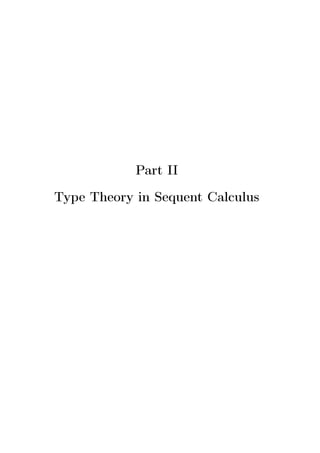

![Chapter 8
Pure Type Sequent Calculi (PTSC)
In this chapter, whose contents appeared in [LDM06], we apply to the framework
of Pure Type Systems [Bar92] the insight into the relationship between sequent
calculus and natural deduction developed in the first part of this dissertation and
in previous work such as [Her94, Her95, DP99b, PD98, DU03].
In sequent calculus the proof-search space is often the cut-free fragment,
since the latter usually satisfies the sub-formula property. The sequent calcu-
lus LJT [Her95], has the extra advantage of being closer to natural deduction (a
reflection is established in Chapter 6), and it makes proof-search more determin-
istic than a Gentzen-style sequent calculus. This makes LJT a natural formalism
to organise proof-search in intuitionistic logic [DP99a], and, its derivations being
close to the notion of uniform proofs, LJT can be used to describe proof-search
in pure Prolog and some of its extensions [MNPS91]. The corresponding term
assignment system also expresses the intimate details of β-normalisation in λ-
calculus in a form closer to abstract (stack-based) machines for reduction (such
as Krivine’s [Kri]).
The framework of Pure Type Systems (PTS) [Bar92] exploits and generalises
the Curry-Howard correspondence, and accounts for many systems already exist-
ing, starting with Barendregt’s Cube. Proof assistants based on them, such as the
Coq system [Coq] or the Lego system [LP92], feature interactive proof construc-
tion methods using proof-search tactics. Primitive tactics display an asymmetry
between introduction rules and elimination rules of the underlying natural de-
duction calculus: the tactic Intro corresponds to the right-introduction rule for
the Π-type (whether in natural deduction or in sequent calculus), but the tactics
Apply in Coq or Refine in Lego are much closer (in spirit) to the left-introduction
of Π-types (as in sequent calculus) than to elimination rules of natural deduc-
tion [McK97].
Although encodings from natural deduction to sequent calculus and vice-versa
have been widely studied [Gen35, Pra65, Zuc74], the representation in sequent
calculus of type theories is relatively undeveloped compared to the literature
about type theory in natural deduction. An interesting approach to PTS using
217](https://image.slidesharecdn.com/frenchenglish-150412084606-conversion-gate01/85/French-english-241-320.jpg)
![218 Chapter 8. Pure Type Sequent Calculi (PTSC)
sequent calculus is in [GR03b]. Nevertheless, only the typing rules are in a
sequent calculus style, whereas the syntax is still in a natural deduction style:
in particular, proofs are denoted by λ-terms, the structure of which no longer
matches the structure of proofs.
However, proofs in sequent calculus can be reflected by specific proof-terms;
for instance, a construction M ·l, representing a list of terms with head M and tail
l, is introduced in [Her94, Her95] to denote the left-introduction of implication
(in the sequent calculus LJT):
Γ M :A Γ; B l:C
Γ; A → B M · l:C
This approach is extended to the corner of the Cube with dependent types and
type constructors in [PD98], but types are still built with λ-terms, so the system
extensively uses conversion functions from sequent calculus to natural deduction
and back.
With such term assignment systems, cut-elimination can be done by means
of a rewrite system, cut-free proofs being thus denoted by terms in normal form.
In type theory, not only is the notion of proof-normalisation/cut-elimination in-
teresting on its own, but it is even necessary to define the notion of typability, as
soon as types depend on terms.
In this chapter we enrich the sequent calculus LJT into a collection of systems
called Pure Type Sequent Calculi (PTSC), capturing the traditional PTS, with
the hope to improve the understanding of implementation of proof systems based
on PTS in respect of:
• having a direct analysis of the basic proof-search tactics, which could then
be moved into the kernel, rather than requiring a separate type-checking
layer for correctness,
• opening the way to improve the basic system with an approach closer to
abstract machines to express reductions, both in type-checking and in ex-
ecution (of extracted programs),
• studying extensions to systems involving inductive types/families (such as
the Calculus of Inductive Constructions).
In fact, the idea of using LJT to describe basic proof-search tactics in Lego was
earlier raised in [McK97]. Here we formalise and develop this approach.
Inspired by the fact that, in type theory, implication and universal quantifica-
tion are just a dependent product, we modify the inference rule above to obtain
the left-introduction rule for a Π-type in a PTSC:
Γ M :A Γ; M/x B l:C
Πl
Γ; ΠxA
.B M · l:C](https://image.slidesharecdn.com/frenchenglish-150412084606-conversion-gate01/85/French-english-242-320.jpg)
![8.1. Syntax reduction 219
We use here explicit substitutions, whose natural typing rule are cuts [BR95].
From our system a version with implicit substitutions can be derived (see Chap-
ter 9), but this does not allow cuts on an arbitrary formula of a typing environ-
ment Γ. Also, explicit substitutions allow the definition of a normalisation proce-
dure by local (small-step) rewrite rules in the spirit of Gentzen’s cut-elimination.
We establish the logical equivalence between a PTSC and its corresponding
PTS by means of type-preserving encodings. We also prove that the former is
strongly normalising if and only if the latter is. The proof is based on mutual en-
codings that allow the normalisation procedure of one formalism to be simulated
by that of the other. Part of the proof also uses a technique by Bloo and Geu-
vers [BG99], introduced to prove strong normalisation properties of the explicit
substitution calculus λx and later used in [DU03] for λ [Her95].
Section 8.1 presents the syntax of a PTSC and gives the rewrite rules for
normalisation. Section 8.3 gives the typing system with the parameters specifying
the PTSC, and a few properties are stated such as subject reduction. Section 8.4
establishes the correspondence between a PTSC and its corresponding PTS, from
which we derive confluence. Section 8.5 presents the strong normalisation result.
8.1 Syntax reduction
Definition 114 (Grammar of PTSC) The syntax of a PTSC depends on a
given set S of sorts, written s, s , . . ., and a denumerable set X of variables,
written x, y, z, . . ..
The set T of terms (denoted M, N, P, . . .) and the set L of lists (denoted
l, l , . . .) are inductively defined as
M, N, A, B ::= ΠxA
.B | λxA
.M | s | x l | M l | M/x N
l, l ::= [] | M · l | l@l | M/x l
ΠxA
.M, λxA
.M, and N/x M bind x in M, and M/x l binds x in l, thus
defining the free variables of terms and lists as well as α-conversion. The set
of free variables of a term M (resp. a list l) is denoted FV(M) (resp. FV(l)).
ΠxA
.M is called a Π-type. Let A→B denote ΠxA
.B when x ∈ FV(B).
This syntax is an extension of Herbelin’s λ [Her95] (with type annotations on
λ-abstractions) presented in Chapter 6. An intuitive understanding of λ in terms
of functions, arguments, abstract machines is presented therein. Note that the
list with head M and tail l, denoted M · l, now has a typing rule corresponding
to the left-introduction of Π-types (cf. Section 8.3). Explicit substitutions will
here be used in two ways: first, to instantiate a universally quantified variable,
and second, to describe explicitly the interaction between the constructors in
the normalisation process, shown in Fig. 8.1. Side-conditions to avoid variable
capture and liberation can be inferred by the process described in Definition 42.](https://image.slidesharecdn.com/frenchenglish-150412084606-conversion-gate01/85/French-english-243-320.jpg)
![220 Chapter 8. Pure Type Sequent Calculi (PTSC)
Confluence of the system is proved in section 8.4. More intuition about λ, its
syntax and operational semantics is also given in [Her95].
B (λxA
.M) (N · l) −→ ( N/x M) l
x
B1 M [] −→ M
B2 (x l) l −→ x (l@l )
B3 (M l) l −→ M (l@l )
A1 (M · l )@l −→ M · (l @l)
A2 []@l −→ l
A3 (l@l )@l −→ l@(l @l )
xsubst:
C1 P/y λxA
.M −→ λx P/y A
. P/y M
C2 P/y (y l) −→ P P/y l
C3 P/y (x l) −→ x P/y l if x = y
C4 P/y (M l) −→ P/y M P/y l
C5 P/y ΠxA
.B −→ Πx P/y A
. P/y B
C6 P/y s −→ s
D1 P/y [] −→ []
D2 P/y (M · l) −→ ( P/y M) · ( P/y l)
D3 P/y (l@l ) −→ ( P/y l)@( P/y l )
Figure 8.1: Reduction Rules
Definition 115 (Convertibility) We say that two terms M and N are con-
vertible if M←→∗
Bx N.
We now show that system x is terminating. If we add rule B, then the system
fails to be terminating unless we only consider terms that are typed in a particular
typing system.
Definition 116 (First-order encoding) We consider the following first-order
signature and its (terminating) precedence relation:
sub(_, _) cut(_, _) ii(_, _) i(_)
The LPO induced on the first-order terms is also terminating. The encoding is
given in Fig. 8.2.
Theorem 202 If M −→x M then MM , and if l −→x l then ll .](https://image.slidesharecdn.com/frenchenglish-150412084606-conversion-gate01/85/French-english-244-320.jpg)
![8.2. A reflection of Pure Type Systems 221
s :=
λxA.M := ii(A, M)
ΠxA.M := ii(A, M)
x l := i(l)
M l := cut(M, l)
M/x N := sub(M, N)
[] :=
M · l := ii(M, l)
l@l := ii(l, l )
M/x l := sub(M, l)
Figure 8.2: Encoding to the first-order syntax
Proof: By induction on M, l. The case analysis for root reduction gives:
B1 cut(M, ) M
B2 cut(i(l), l ) i(ii(l, l ))
B3 cut(cut(M, l), l ) cut(M, ii(l, l ))
A1 ii(ii(M, l ), l) ii(M, ii(l , l))
A2 ii( , l) l
A3 ii(ii(l, l ), l ) ii(l, ii(l , l ))
C1 sub(P, ii(A, M)) ii(sub(P, A), sub(P, M))
C2 sub(P, i(l)) cut(P, sub(P, l))
C3 sub(P, i(l)) i(sub(P, l))
C4 sub(P, cut(M, l)) cut(sub(P, M), sub(P, l))
C5 sub(P, ii(A, B)) ii(sub(P, A), sub(P, B))
C6 sub(P, s)
D1 sub(P, )
D2 sub(P, (ii(M, l))) ii((sub(P, M)), (sub(P, l)))
D3 sub(P, ii(l, l )) ii(sub(P, l), sub(P, l ))
P
Corollary 203 System x is terminating (on all terms and lists).
8.2 A reflection of Pure Type Systems
In this section we establish a reflection in PTSC of Pure Type Systems [Bar92].
Section 8.4 will establish a logical correspondence between a PTSC and a PTS,
in that the following encodings, which form the reflection, preserve a notion of
typing that is given in the next sections.](https://image.slidesharecdn.com/frenchenglish-150412084606-conversion-gate01/85/French-english-245-320.jpg)
![222 Chapter 8. Pure Type Sequent Calculi (PTSC)
We briefly recall the syntax and operational semantics of a PTS. See e.g. [Bar92]
for more detail.
Definition 117 (Syntax reduction of a PTS) The terms have the follow-
ing syntax:
t, u, v, T, U, V, . . . ::= x | s | ΠxT
.t | λxT
.t | t u
where x ranges over variables and s over sorts (as in PTSC).
The calculus is equipped with the β-reduction rule (λxU
.t) u −→β {u
x}t,
which is confluent.
A(s) := s
A(ΠxT
.U) := ΠxA(T)
.A(U)
A(λxT
.t) := λxA(T)
.A(t)
A(t) := A[](t) otherwise
Al(t u) := AA(u)·l(t)
Al(x) := x l
Al(t) := A(t) l otherwise
Figure 8.3: From a PTS to a PTSC
The translation from a PTS to a PTSC is given in Fig. 8.3. It is simply
the adaptation to the higher-order case of Prawitz’s translation from natural
deduction to sequent calculus from Chapter 2: the encoding of an application
relies on a parameterised version of the translation.
B(ΠxA
.B) := ΠxB(A)
.B(B)
B(λxA
.M) := λxB(A)
.B(M)
B(s) := s
B(x l) := {x
z}Bz
(l) z fresh
B(M l) := B(M)
z Bz
(l) z fresh
B( P/x M) := B(P)
x B(M)
By
([]) := y
By
(M · l) := y B(M)
z Bz
(l) z fresh
By
(l@l ) := By(l)
z Bz
(l ) z fresh
By
( P/x l) := B(P)
x By
(l)
Figure 8.4: From a PTSC to a PTS
Fig. 8.4 shows the encoding from a PTSC to a PTS.
Now we want to show that B and A form a reflection in PTSC of PTS. We
first prove the following results:](https://image.slidesharecdn.com/frenchenglish-150412084606-conversion-gate01/85/French-english-246-320.jpg)
![8.2. A reflection of Pure Type Systems 223
Lemma 204
1. A(t) and Al(t) are always x-normal forms (provided l is).
2. If l −→Bx l then Al(t) −→Bx Al (t).
3. Al (t) l−→∗
x Al @l(t) and A(t) l−→∗
x Al(t).
4. A(u)/x A(t)−→∗
x A({u
x}t) and A(u)/x Al(t)−→∗
x A A(u)/x l({u
x}t).
Proof: Each of the above points is obtained by straightforward inductions on
t. P
Now we study the composition of the two encodings:
Lemma 205 Suppose M and l are x-normal forms.
1. If t = x or t = t1 t2 or l = [], then Al(t) = A({t
x}Bx
(l)) if x /∈ FV(l).
2. M = A(B(M)).
Proof: By simultaneous induction on l and M. P
Theorem 206 (A reflection of PTS in PTSC)
1. −→Bx strongly simulates −→β through A.
2. B and A form a reflection in PTSC of PTS.
Proof:
1. If t −→β u then A(t)−→+
Bx A(u) and Al(t)−→+
Bx Al(u), which are proved
by induction on the derivation step, using Lemma 204.4 for the base case
and Lemma 204.3.
2. • The first simulation is given by point 1.
• If M −→B N then B(M)−→∗
β B(N), if l−→B l then By
(l)−→∗
β By
(l ),
if M −→x N then B(M) = B(N) and if l −→x l then By
(l) = By
(l ),
which are proved by simultaneous induction on the derivation step and
case analysis.
• M−→∗
x A(B(M)) holds by induction in SNx
(because x is terminating):
by Lemma 205.2 it holds if M is an x-normal form, and if M −→x N
then we can apply the induction hypothesis on N and by point 2 we
have B(M) = B(N).
• B(A(t)) = t and B(Al(t)) = {t
x}Bx
(l) (with x = FV(l)) are obtained
by simultaneous induction on t.
P](https://image.slidesharecdn.com/frenchenglish-150412084606-conversion-gate01/85/French-english-247-320.jpg)
![224 Chapter 8. Pure Type Sequent Calculi (PTSC)
Now we use Theorem 206 to prove the confluence of PTSC and the equivalence
of the equational theories.
Corollary 207 (Confluence) −→x and −→Bx are confluent.
Proof: From Theorems 5 and 206. P
Corollary 208 (Equational theories)
1. t←→∗
β u if and only if A(t)←→∗
Bx A(u).
2. M←→∗
Bx N if and only if B(M)←→∗
β B(N).
8.3 Typing system properties
Given the set S of sorts, a particular PTSC is specified by a set A ⊆ S2
and a
set R ⊆ S3
. We shall see an example in section 8.5.
Definition 118 (Environments)
• In this chapter, environments, denoted Γ, ∆, Π, . . . are lists of pairs from
X × T denoted x : A. If a pair x:A is an element of an environment Γ, we
also write (x : A) ∈ Γ.
• We define the domain of an environment and the application of a substitu-
tion to an environment by induction on the environment as follows:
Dom([]) := [] P/y ([]) := []
Dom(Γ, x : A) := Dom(Γ), x P/y (Γ, x:A) := P/y Γ, x: P/y A
The domain of an environment is thus a list, but again we allow the notation
x ∈ Dom(Γ) as if it were a set, as well as Dom(Γ) ∩ Dom(∆) which is the
set {x ∈ X | x ∈ Dom(Γ) ∧ x ∈ Dom(∆)}.
• We define the following sub-environment relation:
Γ ∆ if for all (x : A) ∈ Γ, there is (x : B) ∈ ∆ with A←→∗
Bx B.
The inference rules in Fig. 8.5 inductively define the derivability of three kinds
of judgement: some of the form Γ wf, some of the form Γ M :A and some of the
form Γ; B l:A. In the last two cases we call these judgements sequents. In the
last case, B is said to be in the stoup of the sequent, according to a terminology
due to Girard. Side-conditions are used, such as (s1, s2, s3) ∈ R, x ∈ Dom(Γ),
A←→∗
Bx B or ∆ Γ, and we use the abbreviation ∆ Γ wfPTSC for ∆ Γ
and Γ wfPTSC. Derivability in a PTSC of the three kinds of judgement is denoted
Γ wfPTSC, Γ PTSC M :A, and Γ; B PTSC l:A, respectively.](https://image.slidesharecdn.com/frenchenglish-150412084606-conversion-gate01/85/French-english-248-320.jpg)
![8.3. Typing system properties 225
empty
[] wf
Γ A:s x /∈ Dom(Γ)
extend
Γ, x:A wf
Γ A:s
ax
Γ; A []:A
Γ ΠxA
.B :s Γ M :A Γ; M/x B l:C
Πl
Γ; ΠxA
.B M · l:C
Γ; C l:A Γ B :s A←→∗
Bx B
convr
Γ; C l:B
Γ; A l:C Γ B :s A←→∗
Bx B
convl
Γ; B l:C
Γ; C l :A Γ; A l:B
cut1
Γ; C l @l:B
Γ P :A Γ, x:A, ∆; B l:C Γ, P/x ∆ ∆ wf
cut2
∆ ; P/x B P/x l: P/x C
Γ wf (s, s ) ∈ A
sorted
Γ s:s
Γ A:s1 Γ, x:A B :s2 (s1, s2, s3) ∈ R
Πwf
Γ ΠxA
.B :s3
Γ; A l:B (x:A) ∈ Γ
selectx
Γ x l:B
Γ ΠxA
.B :s Γ, x:A M :B
Πr
Γ λxA
.M :ΠxA
.B
Γ M :A Γ B :s A←→∗
Bx B
convr
Γ M :B
Γ M :A Γ; A l:B
cut3
Γ M l:B
Γ P :A Γ, x:A, ∆ M :C Γ, P/x ∆ ∆ wf
cut4
∆ P/x M :C
where either (C = C ∈ S) or C ∈ S and C = P/x C
Figure 8.5: Typing rules of a PTSC](https://image.slidesharecdn.com/frenchenglish-150412084606-conversion-gate01/85/French-english-249-320.jpg)
![226 Chapter 8. Pure Type Sequent Calculi (PTSC)
Since the substitution of a variable in an environment affects the rest of the
environment (which could depend on the variable), the two rules for explicit sub-
stitutions cut2 and cut4 must have a particular shape that is admittedly complex:
thinning (Lemma 212) is built-in by allowing a controlled change of environment.
This may appear artificial, but simpler versions that we have tried failed the
thinning property. More generally, typing rules for explicit substitutions in type
theory are known to be a tricky issue (see for instance [Blo01]), often leading
to the failure of subject reduction (Theorem 216). The rules here are sound in
that respect, but more elegant alternatives are still to be investigated, possibly
by enriching the structure of environments as in [Blo01].
The case analysis for C in the rule cut4 is only necessary for Lemma 209.2
to hold in the presence of top sorts (untyped sorts), and is avoided in [Blo01] by
not using explicit substitutions for types in sequents. Here we were attracted by
the uniformity of using them everywhere, the use of implicit substitutions for C
and the stoup of the third premiss of Πl being only a minor variant.
There are three conversion rules convr, convr, and convl in order to deal with
the two kinds of judgement and, for one of them, convert the type in the stoup.
Lemma 209 (Properties of typing judgements) If Γ PTSC M :A (resp.
Γ; B PTSC l : C) then FV(M) ⊆ Dom(Γ) (resp. FV(l) ⊆ Dom(Γ)), and the
following judgements can be derived with strictly smaller typing derivations:
1. Γ wfPTSC
2. Γ PTSC A:s for some s ∈ S, or A ∈ S
(resp. Γ PTSC B :s and Γ PTSC C :s for some s, s ∈ S)
Proof: Straightforward induction on derivations. P
Corollary 210 (Properties of well-formed environments)
1. If Γ, x:A, ∆ wfPTSC then Γ PTSC A:s for some s ∈ S with a strictly smaller
derivation, with x ∈ Dom(Γ) ∪ Dom(∆) and FV(A) ⊆ Dom(Γ)
(and in particular x ∈ FV(A)).
2. If Γ, ∆ wfPTSC then Γ wfPTSC.
Proof:
1. The first point is proved by induction on the length of ∆ (as a list):
The base case, when ∆ is empty, is obtained by rule extend. Otherwise
∆ = ∆ , y : B and by rule extend we get y = x and Γ, x : A, ∆ PTSC A : sB
for some sB ∈ S with a strictly smaller tree. Hence, by Lemma 209.1 we get
Γ, x : A, ∆ wfPTSC with an even smaller tree, on which it suffices to apply
the induction hypothesis.
The facts that FV(A) ⊆ Dom(Γ) and x ∈ FV(A) then come from Lemma 209.](https://image.slidesharecdn.com/frenchenglish-150412084606-conversion-gate01/85/French-english-250-320.jpg)
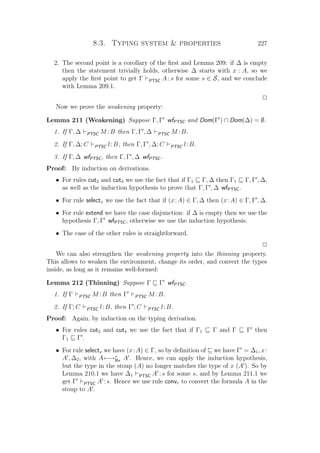
![228 Chapter 8. Pure Type Sequent Calculi (PTSC)
• For rules Πwf and Πr, we want to use the induction hypothesis so we choose
x ∈ Dom(Γ ) and we must prove that Γ, x : A Γ , x : A (which holds by
definition of ) and Γ , x:A wfPTSC. To prove the latter, we use Lemma 209
to get Γ, x:A wfPTSC with a smaller derivation, and Γ PTSC A:s for some s,
with an even smaller derivation, on which we apply the induction hypothesis
and thus get Γ PTSC A:s and then Γ , x:A wfPTSC.
• The case of the other rules is straightforward.
P
For the purpose of proving subject reduction we want to prove a lemma called
the Generation Lemma, and for that we need the following definition.
Definition 119 (Derived without conversion) We write Γ ∗
PTSC M :A (resp.
Γ; B ∗
PTSC l : A) whenever we can derive Γ PTSC M : A (resp. Γ; B PTSC l : A)
and the last rule is not a conversion rule.
In contrast to proof systems in propositional logic, the generation lemma is
non-trivial:
Lemma 213 (Generation Lemma)
1. (a) If Γ PTSC s:C then there is s such that Γ ∗
PTSC s:s with C←→∗
Bx s .
(b) If Γ PTSC ΠxA
.B :C then there is s such that Γ ∗
PTSC ΠxA
.B :s with
C←→∗
Bx s.
(c) If Γ PTSC λxA
.M :C then
there is B such that C←→∗
Bx ΠxA
.B and Γ ∗
PTSC λxA
.M :ΠxA
.B.
(d) If Γ PTSC M/x N :C then there is C such that Γ ∗
PTSC M/x N :C
with C←→∗
Bx C .
(e) If M is not of the above forms and Γ PTSC M :C, then Γ ∗
PTSC M :C.
2. (a) If Γ; B PTSC []:C then B←→∗
Bx C.
(b) If Γ; D PTSC M · l:C then
there are A, B such that D←→∗
Bx ΠxA
.B and Γ; ΠxA
.B ∗
PTSC M · l:C.
(c) If Γ; B PTSC M/x l:C then are B , C such that
Γ; B ∗
PTSC M/x l:C with C←→∗
Bx C and B←→∗
Bx B .
(d) If l is not of the above forms and Γ; D PTSC l:C then Γ; D ∗
PTSC l:C.
Proof: Straightforward induction on the typing tree. P](https://image.slidesharecdn.com/frenchenglish-150412084606-conversion-gate01/85/French-english-252-320.jpg)
![230 Chapter 8. Pure Type Sequent Calculi (PTSC)
with ΠxA
.B←→∗
Bx C←→∗
Bx ΠxD
.E. Hence, A←→∗
Bx D and B←→∗
Bx E.
Moreover, Γ A:sA, Γ, x : A B :sB and Γ wf.
Hence, we get Γ P/x B :sB, so:
Γ P :D
Γ P :A Γ, x : A N :B
Γ P/x N : P/x B
Γ; P/x E l1 :F
Γ; P/x B l1 :F
Γ ( P/x N l1):F
with P/x B←→∗
Bx P/x E.
As A1 (N · l1)@l2 −→ N · (l1@l2)
By the Generation Lemma 2.(b), there are A and B such that
H←→∗
Bx ΠxA
.B and:
Γ ΠxA
.B :s Γ N :A Γ; N/x B l1 :C
Γ; H N · l1 :C Γ; C l2 :F
Γ; H ∗
(N · l1)@l2 :F
Hence,
Γ H :sH
Γ ΠxA
.B :s Γ N :A
Γ; N/x B l1 :C Γ; C l2 :F
Γ; N/x B l1@l2 :C
Γ; ΠxA
.B N · (l1@l2):F
Γ; H N · (l1@l2):F
A2 []@l1 −→ l1
By the Generation Lemma 2.(a), we have A←→∗
Bx H and
Γ; H []:A Γ; A l1 :F
Γ; H ∗
[]@l1 :F
Since Γ H :sH, we get
Γ; A l1 :F
Γ; H l1 :F
A3 (l1@l2)@l3 −→ l1@(l2@l3)
By the Generation Lemma 2.(d),
Γ; H l1 :B Γ; B l2 :A
Γ; H ∗
l1@l2 :A Γ; A l3 :F
Γ; H ∗
(l1@l2)@l3 :F
Hence,
Γ; H l1 :B
Γ; B l2 :A Γ; A l3 :F
Γ; B l2@l3 :F
Γ; H l1@(l2@l3):F](https://image.slidesharecdn.com/frenchenglish-150412084606-conversion-gate01/85/French-english-254-320.jpg)
![8.3. Typing system properties 231
Bs B1 N [] −→ N
Γ N :A Γ; A []:F
Γ ∗
N []:F
By the Generation Lemma 2.(a), we have A←→∗
Bx F.
Since Γ F :sF , we get
Γ N :A
Γ N :F
B2 (x l1) l2 −→ x (l1@l )
By the Generation Lemma 1.(e),
Γ; A l1 :B (x : A) ∈ Γ
Γ ∗
x l:B Γ; B l2 :F
Γ ∗
(x l1) l2 :F
Hence,
(x : A) ∈ Γ
Γ; A l1 :B Γ; B l2 :F
Γ; A l1@l2 :F
Γ x (l1@l2):F
B3 (N l1) l2 −→ N (l1@l2)
By the Generation Lemma 1.(e),
Γ N :A Γ; A l1 :B
Γ ∗
N l1 :B Γ; B l2 :F
Γ ∗
(N l1) l2 :F
Hence,
Γ N :A
Γ; A l1 :B Γ; B l2 :F
Γ; A l1@l2 :F
Γ N (l1@l2):F
Cs We have a redex of the form Q/y R typed by:
∆ Q:E ∆ , y : E, ∆ R:F ∆ , Q/y ∆ Γ wf
Γ ∗
Q/y R:F
with either F = F ∈ S or F = Q/y F .
In the latter case, Γ F :sF for some sF ∈ S. We also have Γ wf.
Let us consider each rule:
C1 Q/y λxA
.N −→ λx Q/y A
. Q/y N](https://image.slidesharecdn.com/frenchenglish-150412084606-conversion-gate01/85/French-english-255-320.jpg)
![234 Chapter 8. Pure Type Sequent Calculi (PTSC)
Ds We have a redex of the form Q/y l1 typed by:
∆ Q:E ∆ , y : E, ∆; H l1 :F ∆ , Q/y ∆ Γ wf
Γ; H ∗
Q/y l1 :F
with F = Q/y F and H = Q/y H . We also have Γ wf and Γ H : sH
and Γ F :sF .
Let us consider each rule:
D1 Q/y [] −→ []
l1 = []
By the Generation Lemma 2.(a), H ←→∗
Bx F , so H←→∗
Bx F.
Γ H :sH
Γ; H []:H Γ F :sF
H []:F
D2 Q/y (N · l2) −→ ( Q/y N) · ( Q/y l2)
l1 = N · l2
By the Generation Lemma 2.(b), there are A, B such that
H ←→∗
Bx ΠxA
.B and:
∆ , y : E, ∆ ΠxA
.B :s ∆ , y : E, ∆ N :A ∆ , y : E, ∆; N/x B l2 :F
∆ , y : E, ∆; ΠxA
.B ∗
l1 :F
From ∆ , y : E, ∆; N/x B l2 :F we get
Γ; Q/y N/x B Q/y l2 :F
From ∆ , y : E, ∆ N :A we get Γ Q/y N : Q/y A.
From ∆ , y : E, ∆ ΠxA
.B : s the Generation Lemma 1.(b) provides
∆ , y : E, ∆ A:sA and ∆ , y : E, ∆, x:A B :sB. Hence we get
∆ , y : E, ∆ A:sA
Γ Q/y A:sA
and thus Γ, x: Q/y A wf and then
∆ , y : E, ∆, x:A B :sB
Γ, x: Q/y A Q/y B :sB
From that we get both Γ Πx Q/y A
. Q/y B :s and
Γ Q/y N/x Q/y B :sB.](https://image.slidesharecdn.com/frenchenglish-150412084606-conversion-gate01/85/French-english-258-320.jpg)
![8.4. Correspondence with Pure Type Systems 235
Note that Πx Q/y A
. Q/y B←→∗
Bx Q/y ΠxA
.B←→∗
Bx Q/y H = H.
We get
Γ Q/y N : Q/y A
Γ; Q/y N/x B Q/y l2 :F
Γ; Q/y N/x Q/y B Q/y l2 :F
Γ; Πx Q/y A
. Q/y B ( Q/y N) · ( Q/y l2):F
Γ; H ( Q/y N) · ( Q/y l2):F
D3 Q/y (l2@l3) −→ ( Q/y l2)@( Q/y l3)
l1 = l2@l3
By the Generation Lemma 2.(d),
∆ , y : E, ∆; H l2 :A ∆ , y : E, ∆; A l3 :F
∆ , y : E, ∆; H ∗
l2@l3 :F
Hence,
Γ; H Q/y l2 : Q/y A Γ; Q/y A Q/y l3 :F
Γ; H ( Q/y l2)@( Q/y l3):F
P
8.4 Correspondence with Pure Type Systems
In this section we establish a logical correspondence between a PTSC given by
the sets S, A and R and the PTS given by the same sets.
Definition 120 (Environments judgements of PTS) Environments of
PTS are lists of pairs such as (x : T) (with T being a PTS-term) and are de-
noted Γ, ∆, Π, . . .. Judgements of PTS are of two kinds: Γ wf, and Γ t:T.
Definition 121 (PTS) The derivable judgements of a PTS specified by the sets
S, A and R are given by the typing rules of Fig. 8.4 and denoted Γ wfPTS and
Γ PTS t:T.
PTS satisfy the following properties:
Theorem 217 (Theorems about PTS)
1. If Γ PTS t:T and Γ ∆ wfPTS then ∆ PTS t:T (where the relation is
defined similarly to that of PTSC, but with β-equivalence).
2. If Γ PTS t:T and Γ, y : T, ∆ PTS u:U
then Γ, {t
y}∆ PTS {t
y}u:{t
y}U.
3. If Γ PTS t:T and t −→β u then Γ PTS u:T.
Proof: See e.g. [Bar92]. P](https://image.slidesharecdn.com/frenchenglish-150412084606-conversion-gate01/85/French-english-259-320.jpg)
![236 Chapter 8. Pure Type Sequent Calculi (PTSC)
[] wf
Γ T :s x /∈ Dom(Γ)
Γ, x:T wf
Γ wf (s, s ) ∈ A
Γ s:s
Γ U :s1 Γ, x:U T :s2 (s1, s2, s3) ∈ R
Γ ΠxU
.T :s3
Γ ΠxU
.T :s Γ, x:U t:T
Γ λxU
.t:ΠxU
.T
Γ t:ΠxU
.T Γ u:U
Γ t u:{u
x}T
Γ wf (x:T) ∈ Γ
Γ x:T
Γ t:U Γ V :s U←→∗
β V
Γ t:V
Figure 8.6: Typing rules of a PTS
Definition 122 (Encoding of environments) We now extend to environments
the encodings between terms of PTS and terms of PTSC:
A([]) := [] B([]) := []
A(Γ, x:T) := A(Γ), x:A(T) B(Γ, x:A) := B(Γ), x:B(A)
Preservation of typing can now be established:
Theorem 218 (Preservation of typing 1)
1. If Γ PTS t:T and Γ; A(T) PTSC l:C then A(Γ) PTSC Al(t):C.
2. If Γ PTS t:T then A(Γ) PTSC A(t):A(T).
3. If Γ wfPTS then A(Γ) wfPTSC.
Proof: By induction on derivations:
1. • For the typing rule of the application, we have t = t1 t2. The other
hypothesis we have is A(Γ); A({t2
x}U) PTSC l:C.
Applying the i.h. on the premisses of the typing rule for application
we get A(Γ) PTSC A(t1):ΠxA(T)
.A(U) and A(Γ) PTSC A(t2):A(T).
By Lemma 209 we get A(Γ) PTSC ΠxA(T)
.A(U):s for some s.
By Lemma 213 we get A(Γ), x:A(T) PTSC A(U):s for some s .](https://image.slidesharecdn.com/frenchenglish-150412084606-conversion-gate01/85/French-english-260-320.jpg)
![8.4. Correspondence with Pure Type Systems 237
By rule cut4 we get A(Γ) PTSC A(t2)/x A(U):s .
By Theorem 206.1 we get A(t2)/x A(U)←→∗
Bx A({t2
x}U). Hence,
A(Γ) PTSC A(t2):A(T)
A(Γ); A( t2
x U) PTSC l:C
A(Γ); A(t2)/x A(U) PTSC l:C
A(Γ); ΠxA(T)
.A(U) PTSC A(t2) · l:C
and then we can conclude by applying point 1 of the i.h. on t1.
• The case of the other rules is straightforward.
2. • For the typing rule of the application, we have t = t1 t2:
By point 2 of the i.h. we get again A(Γ) PTSC A(t1) : ΠxA(T)
.A(U)
and A(Γ) PTSC A(t2):A(T).
As for point 1 we get A(Γ) PTSC A(t2)/x A(U):s .
By Theorem 206.1 and subject reduction (Theorem 216) we get
A(Γ) PTSC A({t2
x}U):s, from which we can derive
A(Γ); A({t2
x}U) PTSC [] : A({t2
x}U) and we can apply the first
point.
• For the axiom, we have t = x, with x:T in the environment Γ wfPTS:
Point 3 of the i.h. gives A(Γ) wfPTSC, so by Lemma 210 and Lemma 211
we get A(Γ) PTSC A(T) : s for some s. We can then derive
A(Γ); A(T) PTSC []:A(T) and A(Γ) PTSC x []:A(T).
• The case of the other rules is straightforward.
3. All cases are straightforward.
P
Theorem 219 (Preservation of typing 2)
1. If Γ PTSC M :A then B(Γ) PTS B(M):B(A)
2. If Γ; B PTSC l:A then B(Γ), y : B(B) PTS By
(l):B(A) for a fresh y
3. If Γ wfPTSC then B(Γ) wfPTS
Proof: Straightforward induction on derivations, using Theorem 217. P](https://image.slidesharecdn.com/frenchenglish-150412084606-conversion-gate01/85/French-english-261-320.jpg)
![238 Chapter 8. Pure Type Sequent Calculi (PTSC)
8.5 Equivalence of strong normalisation
Theorem 220 A PTSC given by the sets S, A, and R is strongly normalising
if and only if the PTS given by the same sets is.
Proof: Assume that the PTSC is strongly normalising, and let us consider
a typed term t of the corresponding PTS, i.e. Γ PTS t : T for some Γ, T. By
Theorem 218, A(Γ) A(t) : A(T) so A(t) ∈ SNBx
. Hence, by Theorem 206.1
and Theorem 22, t ∈ SNβ
.
Now assume that the PTS is strongly normalising and that Γ M : A in
the corresponding PTSC. We shall now apply Bloo and Geuvers’ technique
from [BG99]. By subject reduction, any N such that M−→∗
Bx N satisfies Γ N :
A and any sub-term P (resp. sub-list l) of any such N is also typable. By Theo-
rem 219, for any such P (resp. l), B(P) (resp. By
(l)) is typable in the PTS, so it
is strongly normalising by assumption and we denote by B(P) (resp. By
(l)) the
length of the longest β-reduction sequence reducing it.
We now encode any such P and l into a first-order syntax given by the fol-
lowing infinite signature and its precedence relation:
subn
(_, _) cutn
(_, _) ii(_, _) i(_)
for all integers n. Moreover, we set subn
(_, _) cutm
(_, _) if n m. The
precedence relation is terminating, and the LPO that it induces on the first-order
terms is also terminating (Theorem 49). The encoding is given in Fig 8.7.
s :=
λxA.M := ii(A, M)
ΠxA.M := ii(A, M)
x l := i(l)
M l := cut B(M l)
(M, l)
M/x N := sub B( M/x N)
(M, N)
[] :=
M · l := ii(M, l)
l@l := ii(l, l )
M/x l := sub By( M/x l)
(M, l) where y is fresh
Figure 8.7: Encoding into the first-order syntax
An induction on terms shows that reductions decrease the LPO:
B cutn
(ii(A, M), ii(N, l))cutn
(subm
(N, M), l)
where n = (λxB(A).B(M)) B(N)
y By
(l) {B(N)
x}B(M)
y By
(l) = n
and n B(N)
x B(M) = m.](https://image.slidesharecdn.com/frenchenglish-150412084606-conversion-gate01/85/French-english-262-320.jpg)
![240 Chapter 8. Pure Type Sequent Calculi (PTSC)
Examples of strongly normalising PTS are the eight corners of Barendregt’s
Cube [Bar92], the collection of PTS given by the following sets:
S := {P0, P1}
A := {(P0, P1)}
{(P0, P0, P0)} ⊆ R ⊆ {(P0, P0, P0), (P0, P1, P1), (P1, P0, P0), (P1, P1, P1)}
The three dimensions of the Cube correspond to the properties (P0, P1, P1) ∈ R
(dependent types), (P1, P0, P0) ∈ R (polymorphism), and (P1, P1, P1) ∈ R (type
constructors), which can be combined in eight different ways.
Among these systems are the simply-typed λ-calculus, system F, system Fω,
their respective versions with dependent types such as the Calculus of
Constructions [CH88] (CoC), which combines the three dimensions with
R = {(P0, P0, P0), (P0, P1, P1), (P1, P0, P0), (P1, P1, P1)}.
The latter can be extended into the PTS given by following sets, which is still
strongly normalising:
S := {P0, P1, . . . , Pi, . . .}
A := {(Pi, Pi+1)| i ∈ N}
R ⊆ {(Pi, Pj, Pmax(i,j))| i, j ∈ N} ∪ {(Pi, P0)| i ∈ N}
This is the Calculus of Constructions with Universes [Luo90], on which the proof-
assistant Coq is based [Coq] (but it also uses inductive types and local definitions).
For each of the above PTS we now have a strongly normalising and logically
equivalent sequent calculus, namely the PTSC given by the same sets S, A and
R, which can be used for proof-search as we shall see in the next chapter. We
thus have for instance the Sequent Calculus of Constructions and the Sequent
Calculus of Constructions with Universes.
Conclusion
We have defined a parameterised formalism that gives a sequent calculus for each
PTS. It comprises a syntax, a rewrite system and typing rules. In contrast to
previous work, the syntax of both types and proof-terms of PTSC is in a sequent-
calculus style, thus avoiding the use of implicit or explicit conversions to natural
deduction [GR03b, PD98].
A strong correspondence with natural deduction has been established (in par-
ticular, regarding both the logic and the strong normalisation), and for instance
we derive from it the confluence of each PTSC. We can give as examples the
corners of Barendregt’s Cube.
The sequent calculus that we have used is based on LJT because of its well-
known connections with natural deduction, in particular it is permutation-free,
in that its x-normal forms are in bijection with λ-terms, with the same equational
theory on them.](https://image.slidesharecdn.com/frenchenglish-150412084606-conversion-gate01/85/French-english-264-320.jpg)
![Conclusion 241
However this raises the question of whether a type theory can be built on
a Gentzen-style sequent calculus such as G3ii. In that case, various options are
possible for the equational theory that is used in the conversion rules: we can
either include therein the permutations of those sequent calculus proof-terms
that correspond to identical λ-terms, or not. Draft work in my research has
shown that both options are possible, leading to different (probably syntactic and
uninteresting) models. However we do not include the Gentzen-style approach in
this dissertation because it is highly technical, while less inelegant alternatives
are to be sought, maybe using Espirito Santo’s approach [EFP06].
Also, it would be interesting to have direct proofs of strong normalisation for
particular PTSC, such as the Sequent Calculus of Constructions. This could be
based on [Kik04a], which adapts Tait’s [Tai75] method to the particular PTSC
corresponding to propositional logic.
Further work includes the investigation of inductive types in sequent calculus,
such as those used in Coq. Finally, sequent calculus is also more elegant than
natural deduction to express classical logic, so it would be interesting to build
classical Pure Type Sequent Calculi.](https://image.slidesharecdn.com/frenchenglish-150412084606-conversion-gate01/85/French-english-265-320.jpg)

![244 Chapter 9. Variants of PTSC
to the Constructive engine in natural deduction [Hue89, vBJMP94]. However
the latter is used for type synthesis, whose inputs and outputs are different from
those of proof synthesis and lead to a different way to integrate conversion rules,
as discussed further. In section 9.1 the version of PTSC optimised for proof
synthesis is proved equivalent to the PTSC, i.e. sound and complete in a strong
sense that we shall make precise. We illustrate the use of the proof synthesis
version of PTSC with an example.
To the root-first application of our optimised rules we can then compare some
basic proof search tactics of proof assistants based on PTS, most interestingly
the tactics Apply in Coq or Refine in Lego. As mentioned in the introduction of
Chapter 8 and noticed by [McK97] long before, these are much closer (in spirit)
to the left-introduction of Π-types (as in rule Πl below) than to elimination rules
of natural deduction.
Γ M :A Γ; M/x B l:C
Πl
Γ; ΠxA
.B M · l:C
However these tactics are also able to postpone the investigation of the first
premiss of the rule and start investigating the second, using unification constraints
instead of simple conversions. Moreover, [Dow93] shows that in type theories such
as the Calculus of Constructions [CH88], the process of proof synthesis merges
with that of unification [Hue76].
While [McK97] investigates the aforementioned postponement of the resolu-
tion of the first premiss by using Lego’s local definition mechanism [LP92], we
show in section 9.2 that the sequent calculus approach is also convenient to ex-
press proof synthesis algorithms such as those of [Dow93, Mun01]. This is done
by extending the syntax of PTSC with higher-order variables, which have the
same role as meta-variables added to the object-level syntax, in that they repre-
sent unknown proof-terms yet to be found. These variables are used to postpone
recursive calls of the proof synthesis procedure as well as in the unification con-
straints. Further development of this part seems to represent some of the most
promising directions for future work.
Type synthesis is the process that takes as an input an environment Γ and
a term M and that produces as an output a type A such that Γ M : A. The
recursive calls of the process will also take, as inputs, an environment Γ, a type
B and a list l, and produce, as an output, a type A such that Γ; B l:A. They
will also take an environment Γ as an input and answer whether or not it is well-
formed. These three kinds of input/output behaviour naturally correspond to the
three kinds of judgements as in Fig. 8.5. Again, an inference system that defines
such a procedure by root-first application of its rules is also syntax-directed, but
this time, since the inputs and outputs are different from those of proof synthesis,
the rules are directed by the syntax of the term which is the input (as well as
using the information given in the environment). Note that in the typing system
of PTSC (Fig. 8.5), what makes the rules non-syntax-directed is:](https://image.slidesharecdn.com/frenchenglish-150412084606-conversion-gate01/85/French-english-268-320.jpg)
![Introduction 245
• the conversion rules, which could apply at any point, with a type A to
invent,
• the shape of the typing rules for explicit substitutions: type synthesis would
need to extract, from an environment Π and a term M, an environment
Γ, x:A, ∆ such that Γ, M/x ∆ Π.
The latter point is as hard as extracting from a substituted term the original
(implicit) substitution that formed it; there are just too many possibilities. This
is naturally connected to the inelegance of our typing rules cut2 and cut4, and
probably the way to make type synthesis work for explicit substitutions is to have
a typing system in which Subject Expansion holds for xsubst: if M −→xsubst N
and Γ N :A then Γ M :A, possibly under some particular conditions. Then,
since xsubst terminates (it is in fact confluent), the process of type synthesis
could produce a type for the xsubst-normal form of its input term, and this
would also be a valid type for the input term. Kervarc and Lescanne [KL04]
develop a version of PTS along these lines, in natural deduction but with a form
of explicit substitution similar to ours. Also in natural deduction is the Calculus
of Constructions with explicit substitutions of [Mun01], but in quite a different
setting that uses de Bruijn indices [dB72] in the style of λσ [ACCL91, CHL96].
Explicit substitutions are of a more advanced/complex kind, forming a syntactic
category of their own, with typing rules that depart from a simple cut in sequent
calculus.
In this dissertation we give in section 9.3 a version of PTSC, called PTSCimp,
that uses implicit substitutions rather than explicit ones. PTSCimp will also be
easier to convert into a version that uses de Bruijn indices.
An inference system for type synthesis can then be defined in section 9.4, based
on PTSCimp. The former point that made the typing system of PTSC (Fig. 8.5)
non-syntax-directed for type synthesis was the presence of the conversion rules,
so the inference system of section 9.4 integrates them into the typing rules of term
constructions. This time, such an integration is exactly the counterpart in sequent
calculus of the constructive engine in natural deduction [Hue89, vBJMP94], which
serves the same purpose of type synthesis. Our system gives the opportunity
to discuss whether normal forms can be typed without cut-rules and raise, in
our framework of sequent calculus, well-known issues related to PTS, such as
Expansion Postponement [Pol92, vBJMP94, Pol98, GR03a].
Finally, in section 9.5 we develop implementation-friendly versions of PTSC
using de Bruijn indices and corresponding to PTSC with implicit substitutions in
two variants: the version optimised for proof synthesis (but not with the extension
of higher-order variables, left as future work), and the version optimised for type
synthesis. It appears that [KR02] developed a version of PTS with de Bruijn
indices, using the very same machinery (same style of indices, reduction. . . ). In
other word, section 9.5 turns out to be the PTSC version of [KR02].](https://image.slidesharecdn.com/frenchenglish-150412084606-conversion-gate01/85/French-english-269-320.jpg)
![246 Chapter 9. Variants of PTSC
9.1 Proof synthesis
In contrast to propositional logic where cut is an admissible rule of sequent calcu-
lus, terms of PTSC in normal form may need a cut-rule in their typing derivation.
For instance in the rule Πl, a type which is not normalised ( M/x B) must ap-
pear in the stoup of the third premiss, so that cuts might be needed to type it
inside the derivation.
In this section we present a system for proof synthesis that avoids all cuts, is
complete and is sound provided that types are checked independently. In proof
synthesis, the inputs are an environment Γ and a type A, henceforth called goal,
and the output is a term M such that Γ M :A. When we look for a list, the type
in the stoup is also an input. The inference rules now need to be directed by the
shape of the goal (or of the type in the stoup), and the proof synthesis system (PS,
for short) can be obtained by optimising the use of the conversion rules as shown in
Fig. 9.1. The incorporation of the conversion rules into the other rules is similar to
that of the Constructive Engine in natural deduction [Hue89, vBJMP94]; however
the latter was designed for type synthesis, for which the inputs and outputs are
not the same as in proof synthesis, as mentioned in the introduction.
A←→∗
Bx A
axPS
Γ; A PS []:A
D−→∗
Bx ΠxA
.B Γ PS M :A Γ; M/x B PS l:C
ΠlPS
Γ; D PS M · l:C
C−→∗
Bx s3 (s1, s2, s3) ∈ R Γ PS A:s1 Γ, x:A PS B :s2
ΠwfPS
Γ PS ΠxA
.B :C
C−→∗
Bx s2 (s1, s2) ∈ A
sortedPS
Γ PS s:C
(x : A) ∈ Γ Γ; A PS l:B
selectx
Γ PS x l:B
C−→∗
Bx ΠxA
.B Γ, x:A PS M :B
ΠrPS
Γ PS λxA
.M :C
Figure 9.1: System PS
We now prove soundness, and for that it is useful to define the following
notion:
Definition 123 A term (or a list) is a quasi normal form if all its redexes are
within type annotations of λ-abstractions, e.g. A in λxA
.M.
System PS is sound in the following sense:](https://image.slidesharecdn.com/frenchenglish-150412084606-conversion-gate01/85/French-english-270-320.jpg)
![9.1. Proof synthesis 249
We now give the example of a derivation in PS. We consider the PTSC equiv-
alent to system F, i.e. the one given by the sets:
S = { , P}, A = {( , P)}, and R = {( , ), (P, )}.
For brevity we omit the types on λ-abstractions, we abbreviate x [] as x for
any variable x and simplify N/x P as P when x ∈ FV(P). We also write A∧B for
ΠQ .(A→(B→Q))→Q. Trying to find a term M such that
A : , B : M :(A ∧ B)→(B ∧ A), we get the PS-derivation below:
πB
Γ PS NB :B
πA
Γ PS NA :A
ax
Γ; Q PS []:Q
Πl
Γ; A→Q PS NA · []:Q
Πl
Γ; B→(A→Q) PS NB · NA · []:Q
selecty
Γ PS y NB · NA · []:Q
============================================== Πr
A : , B : PS λx.λQ.λy.y NB · NA · []:(A ∧ B)→(B ∧ A)
where Γ = A : , B : , x : A ∧ B, Q : , y : B→(A→Q), and πA is the following
derivation (NA = x A · (λx .λy .x ) · []):
Γ; PS []:
Γ PS A:
Γ, x : A, y : B; A PS []:A
Γ, x : A, y : B PS x :A
=======================
Γ PS λx .λy .x :A→(B→A) Γ; A PS []:A
Γ; A/Q (A→(B→Q))→Q PS (λx .λy .x ) · []:A
Γ; A ∧ B PS A · (λx .λy .x ) · []:A
Γ PS x A · (λx .λy .x ) · []:A
and πB is the derivation similar to πA (NB = x B · (λx .λy .y ) · []) with conclusion
Γ PS x B · (λx .λy .y ) · []:B.
This example shows how the non-determinism of proof synthesis is sometimes
quite constrained by the need to eventually unify the type in the stoup with
the goal. For instance in πA (resp. πB), solving Γ Q : must produce A
(resp. B) otherwise the resolution of the right-hand side branch fails. Indeed,
the dependency created by a Π-type forces the resolution of the two premisses of
rule Πl to be sequentialised in a way that might reveal inefficient: the proof-term
produced for the first premiss, selected among others at random, might well lead
to the failure of solving the second premiss, leading to endless backtracking.
Hence, there is much to gain in postponing the resolution of the first pre-
miss and trying to solve the second with incomplete inputs (in our example, not
knowing Q). This might not terminate with success or failure but this will send
back useful constraints that will help the resolution of the first premiss with the](https://image.slidesharecdn.com/frenchenglish-150412084606-conversion-gate01/85/French-english-273-320.jpg)
![250 Chapter 9. Variants of PTSC
right proof-term. “Helping” could just be giving some information to orient and
speed-up the search for the right proof-term, but it could well define it completely
(saving numerous attempts with proof-terms that will lead to failure). Unsurpris-
ingly, these constraints are produced by the axiom rule as unification constraints,
in our example the constraint Q = A for πA and Q = B for πB, which in both
cases define Q entirely indeed.
This is what happens in Coq [Coq], whose proof-search tactic apply x can
be decomposed into the bottom-up application of selectx followed by a series of
bottom-up applications of Πl and finally ax, but it either postpones the resolution
of sub-goals or automatically solves them from the unification attempt, often
avoiding obvious back-tracking.
In the next section we investigate how we can express this behaviour in a
sequent calculus.
9.2 Higher-order variables for proof enumeration
In order to mimic even more closely such a tactic as apply x of Coq, we tackle
in this section the issue of delaying the resolution of sub-goals. Where such a
resolution should have produced a proof-term of the correct type, we now offer
the possibility of “cheating” by producing something similar to a meta-variable
that represents a term yet to be found and that can be manipulated as one.
By thus extending PTSC, we can go further than accounting for a proof-
search tactic such as apply x of Coq and express a sound and complete algo-
rithm for type inhabitant enumeration. This is similar to Dowek’s [Dow93] and
Muñoz’s [Mun01] in natural deduction, but the novelty here is that the algorithm
is simply the root-first construction of derivation trees in sequent calculus.
In fact, instead of meta-variables, we use the possibility, offered by the for-
malism of HOC, of higher-order variables. This is quite similar to CRS [Klo80], in
that unknown terms are represented with (meta/higher-order) variables applied
to the series of (term-)variables that could occur freely in those terms, e.g. α(x, y)
to represent a term M in which x and y could be free. These arguments can later
be instantiated, so that α(N, P) will represent N,P
x,y M. In other words, a
(meta/higher-order) variable on its own represents something closed, e.g. x.y.M
with FV(M) ⊆ {x, y}, using the binding mechanism of HOC (or CRS).
This kind of meta-variable differs from that of in [Mun01], which is rather
in the style of ERS [Kha90] where the variables that could occur freely in the
unknown term are not specified explicitly. The drawback of our approach is that
we have to know in advance the free variables that might occur freely in the
unknown term, but in a typed setting such as proof synthesis these are actually
the variables declared in the environment. Moreover, although specifying explic-
itly the variables that could occur freely in an unknown term might seem heavy,
it actually avoids the well-known problem of non-confluence of reduction when](https://image.slidesharecdn.com/frenchenglish-150412084606-conversion-gate01/85/French-english-274-320.jpg)
![9.2. Proof enumeration 251
terms contain meta-variables in the style of [Mun01]. The solution in [Mun01] has
the drawback of not simulating β-reduction (but the reductions in [Mun01] reach
the expected normal forms). The machinery developed in Chapter 5 might allow
a similar solution but with simulation of β-reduction, however it would be very
heavy and here we simply prefer avoiding the problem by using the CRS-approach
to meta-variables.
Definition 124 (Open terms) The grammar of open terms and open lists is
defined as follows:
M, N, A, B ::= ΠxA
.B | λxA
.M | s | x l | M l | M/x N | α(M1, . . . , Mn)
l, l ::= [] | M · l | l@l | M/x l | β(M1, . . . , Mn)
where α, β range over variables of order 1 and arity n, for all n, respectively
producing terms and lists.
Terms and lists without these variables (i.e. terms and lists of Definition 114)
are now called ground terms and ground lists, respectively.
Definition 125 (Extension of x-reduction) Owing to the presence of higher-
order variables, we have to extend system x with the following rules:
P/y α(M1, . . . , Mn) −→ α( P/y M1, . . . , P/y Mn)
P/y β(M1, . . . , Mn) −→ β( P/y M1, . . . , P/y Mn)
This extended system is called x .
Conjecture 224 (Confluence of Bx ) System Bx is confluent.
Proof: Considering higher-order variables in the style of CRS [Klo80] avoids the
usual problem of non-confluence coming from the critical pair between B and C4
which generate the two terms N/x P/y M and N/x P/y N/x M. Indeed,
with ERS-style meta-variables these two terms need not reduce to a common
term, but with the CRS-approach they now can with the two new rules of x .
The other critical pairs between Bs and C4, as well as the critical pairs between
As and D3, B and B3, As and A3 are also easily joined. The last critical pair is
between B3 and itself (or B2), and for that rule A3 is needed, while it was only
there for convenience when all terms were ground.
Joinability of critical pairs is not sufficient to derive confluence of the (higher-
order) rewrite system, but it gives confidence that a proof can be found. In
fact, it seems that the proof technique for Corollary 207 (confluence of PTSC
with ground terms) can be adapted to the case with open terms: to derive the
confluence result from that of PTS using a reflection we only need to find a
good encoding of our higher-order variables in PTS (this seems to work precisely
because we use CRS-style meta/higher-order variables). The details remain to be
checked. P](https://image.slidesharecdn.com/frenchenglish-150412084606-conversion-gate01/85/French-english-275-320.jpg)
![9.2. Proof enumeration 253
Γ = x1 :A1, . . . , xn :An
Γ; D β(x1 [], . . . , xn []):C | (Γ; D β :C)
Γ; D []:C | D
Γ
←→ C
D−→∗
Bx ΠxA
.B Γ M :A | Σ1 Γ; M/x B l:C | Σ2
Γ; D M · l:C | Σ1, Σ2
Γ = x1 :A1, . . . , xn :An
Γ α(x1 [], . . . , xn []):C | (Γ α:C)
C−→∗
Bx s (s , s) ∈ A
Γ s :C | []
C−→∗
Bx s (s1, s2, s) ∈ R Γ A:s1 | Σ1 Γ, x:A B :s2 | Σ2
Γ ΠxA
.B :C | Σ1, Σ2
(x:A) ∈ Γ Γ; A l:C | Σ
Γ x l:C | Σ
C−→∗
Bx ΠxA
.B Γ, x:A M :B | Σ
Γ λxA
.M :C | Σ
Γ; B l:A | Σ Σ, Σ , Dom(Γ).l
β Σ =⇒ σ
Σ, (Γ; B β :A), Σ =⇒ σ, β → Dom(Γ).σ(l)
Γ M :A | Σ Σ, Σ , Dom(Γ).M
α Σ =⇒ σ
Σ, (Γ α:A), Σ =⇒ σ, α → Dom(Γ).σ(M)
Σ is solved
Σ =⇒ ∅
Figure 9.2: Proof-term enumeration](https://image.slidesharecdn.com/frenchenglish-150412084606-conversion-gate01/85/French-english-277-320.jpg)
![254 Chapter 9. Variants of PTSC
Σ is the input of proof synthesis and σ is meant to be its solution, i.e.
the output. We write σ(M) (resp. σ(l)) for M1,...,Mn
α1,...,αn M (resp.
M1,...,Mn
α1,...,αn l) if σ = α1 → M1, . . . , αn → Mn, and similarly for sub-
stitutions on higher-order variables like β and mixtures of the two kinds.
The inference rules of system PE (for Proof Enumeration) are presented in Fig. 9.2.
Derivability in PE of the three kinds of judgement is denoted Γ PE M : A | Σ,
Γ; B PE M :A | Σ and Σ =⇒PE σ.
Now we prove that PE is sound. For that we need the following notion:
Definition 129 (Solution) We define the property σ is a solution of a goal
environment Σ, by induction on the length of Σ.
• σ is a solution of [].
• If σ is a solution of Σ and
x1 :σ(A1), . . . , xn :σ(An) PS app(σ(α), x1 [], . . . , xn []):σ(A)
then σ is a solution of Σ, (x1 :A1, . . . , xn :An α:A).
• If σ is a solution of Σ and
x1 :σ(A1), . . . , xn :σ(An); σ(B) PS app(σ(β), x1 [], . . . , xn []):σ(A)
then σ is a solution of Σ, (x1 :A1, . . . , xn :An; B β :A).
• If σ is a solution of Σ and
σ(M)←→∗
Bx σ(N)
then σ is a solution of Σ, M
Γ
←→ N.
For soundness we also need the following lemma:
Lemma 225 Suppose that σ(M) and σ(M) are ground.
1. If M −→Bx N then σ(M) −→Bx σ(N).
2. If l −→Bx l then σ(l) −→Bx σ(l ).
Proof: By simultaneous induction on the derivation of the reduction step,
checking all rules for the base case of root reduction. P
Theorem 226 (Soundness) Suppose σ is a solution of Σ.
1. If Γ PE M :A | Σ then σ(Γ) PS σ(M):σ(A).
2. If Γ; B PE M :A | Σ then σ(Γ); σ(B) PS σ(M):σ(A).
Proof: By induction on derivations. P](https://image.slidesharecdn.com/frenchenglish-150412084606-conversion-gate01/85/French-english-278-320.jpg)
![9.2. Proof enumeration 255
Corollary 227 If Σ =⇒PE σ then σ is a solution of Σ.
Proof: By induction on the derivation, using Theorem 226. P
System PE is complete in the following sense:
Theorem 228 (Completeness)
1. If Γ PS M :A then Γ PE M :A | Σ for some solved goal environment Σ.
2. If Γ; B PS M :A then Γ; B PE M :A | Σ for some solved Σ.
Proof: By induction on derivations. The rules of PE generalise those of PS. P
In fact, the completeness of the full system PE is not surprising, since it is
quite general. In particular, nothing is said about when the process should decide
to abandon the current goal and start working on another one. Hence we should
be interested in completeness of particular strategies dealing with that question.
• For instance, PS corresponds to the strategy of eagerly solving sub-goals as
soon as they are created, never delaying them with the sub-goal environ-
ment.
• The algorithm for proof enumeration in [Dow93] would correspond here to
the “lazy” strategy that always abandons the sub-goal generated by rule
ΠlPS, but this in fact enables the unification constraints to give guidance in
solving this sub-goal later, so in that case laziness is probably more efficient
than eagerness. This is probably what should be chosen for automated
theorem proving.
• Mixtures of the two strategies can also be considered and could be the basis
of interactive theorem proving. Indeed in some cases the user’s input might
be more efficient than the automated algorithm, and rule ΠlPS would be a
good place to ask whether the user has any clue to solve the sub-goal (since
it could help solving the rest of the unification). If he or she has none, then
by default the algorithm might abandon the sub-goal and leave it for later.
In Coq, the tactic apply x does something similar: it tries to automatically
solve the sub-goals that interfere with the unification constraint (leaving
the other ones for later, visible to the user), but if the unification fails,
it is always possible for the user to use the tactic and explicitly give the
proof-term that will make it work. However, such an input is not provided
in proof synthesis mode and the user really has to give it fully, since the
tactic will fail if the unification fails. In PE, the unification constraint can
remain partially solved.
All these behaviours can be simulated in PE, which is therefore a useful framework
to study proof synthesis strategies in type theory.](https://image.slidesharecdn.com/frenchenglish-150412084606-conversion-gate01/85/French-english-279-320.jpg)
![256 Chapter 9. Variants of PTSC
9.3 PTSC with implicit substitutions
In this section we define a version of PTSC with implicit substitutions, called
PTSCimp. Note that the notion of implicit substitution from Definition 43 is not
very useful here, since variables form a syntactic category of their own. What
allows the definition of a notion of implicit substitution that corresponds to the
explicit ones of PTSC is that the constructor for x l can turn into the constructor
for M l, which is different.
Definition 130 (The syntax with implicit substitutions) The syntax of
PTSCimp is that of PTSC when we remove explicit substitutions, namely:
M, N, A, B ::= ΠxA
.B | λxA
.M | s | x l | M l
l, l ::= [] | M · l | l@l
These terms and lists are henceforth called substitution-free terms and lists.
Fig. 9.3 defines implicit substitutions on substitution-free terms and lists.
P
y (λxA
.M) := λx{P
y}A
. P
y M
P
y (y l) := P P
y l
P
y (x l) := x P
y l
P
y (M l) := P
y M P
y l
P
y (ΠxA
.B) := Πx{P
y}A
. P
y B
P
y s := s
P
y [] := []
P
y (M · l) := ( P
y M) · ( P
y l)
P
y (l@l ) := ( P
y l)@( P
y l )
Figure 9.3: Implicit substitutions in PTSCimp
As with the notion of substitution from Definition 43, the substitution lemma
holds (Lemma 40):
Lemma 229 (Substitution Lemma)
1. If M, N, P are substitution-free terms, P
y
N
x M = {P
y}N
x
P
y M
2. If l is a substitution-free list and N, P are substitution-free terms,
P
y
N
x l = {P
y}N
x
P
y l
Proof: By induction on M, l. P](https://image.slidesharecdn.com/frenchenglish-150412084606-conversion-gate01/85/French-english-280-320.jpg)
![9.3. PTSC with implicit substitutions (PTSCimp) 257
The following lemma shows that the propagation of explicit substitutions by
th system x of PTSC implements the notion of implicit substitution defined above.
Lemma 230 Provided P, M, l are substitution-free, we have
P/x M−→∗
xsubst
P
x M and P/x l−→∗
xsubst
P
x l.
Proof: By induction on M, l. P
Definition 131 (Reduction system for PTSCimp) The internal reduction sys-
tem of PTSCimp is presented in Fig. 9.4.
B (λxA
.M) (N · l) −→ ( N
x M) l
x
B1 M [] −→ M
B2 (x l) l −→ x (l@l )
B3 (M l) l −→ M (l@l )
A1 (M · l )@l −→ M · (l @l)
A2 []@l −→ l
A3 (l@l )@l −→ l@(l @l )
Figure 9.4: Reduction Rules of PTSCimp
Note that the system x of Fig. 9.4 is but the system x of Fig. 8.1 when all
terms are substitution-free.
Remark 231
1. The syntax of substitution-free terms and lists is stable under −→B x .
2. Moreover, from Lemma 230 we get −→B ⊆ −→∗
Bx , so the rule adds nothing
to the equational theory.
The reduction relation is closed under substitutions in the following sense:
Lemma 232 Provided P, M, l are substitution-free,
1. if P −→B x P then P
x M −→B x
P
x M and P
x l −→B x
P
x l,
2. if M −→B x M then P
x M −→B x
P
x M , and
if l −→B x l then P
x l −→B x
P
x l .
Proof: By induction on M, l, using the Substitution Lemma for point 2 in the
case of root B -reduction. P
Using implicit substitutions we can now “purify” a term to remove its explicit
substitutions. This purification is presented in Fig. 9.5.
Remark 233 If M is substitution-free then ⇓(M) = M.
Lemma 234 M−→∗
xsubst ⇓(M) and l−→∗
xsubst ⇓(l).
Proof: By induction on M, l. P](https://image.slidesharecdn.com/frenchenglish-150412084606-conversion-gate01/85/French-english-281-320.jpg)
![258 Chapter 9. Variants of PTSC
⇓(λxA
.M) := λx⇓(A)
.⇓(M)
⇓(x l) := x ⇓(l)
⇓(M l) := ⇓(M) ⇓(l)
⇓(ΠxA
.B) := Πx⇓(A)
.⇓(B)
⇓(s) := s
⇓( P/y M) := ⇓(P)
y ⇓(M)
⇓([]) := []
⇓(M · l) := (⇓(M)) · (⇓(l))
⇓(l@l ) := (⇓(l))@(⇓(l ))
Figure 9.5: Purification
Theorem 235 (Simulation of Bx by B x through ⇓)
1. If M −→Bx N then ⇓(M)−→∗
B x ⇓(N).
2. If l −→Bx l then ⇓(l)−→∗
B x ⇓(l ).
Proof: By induction on M, l, using Lemma 229. P
Corollary 236 (Reflection in PTSC of PTSCimp) ⇓ and the identity func-
tion form a reflection in PTSC of PTSCimp.
Proof: This is the conjunction of Lemma 230, Remark 233, Lemma 234, and
Theorem 235. P
Corollary 237 (Confluence of PTSCimp) PTSCimp are confluent.
Proof: From Corollary 236 we get that the identity function and ⇓ form a
pre-Galois connection from PTSCimp to PTSC, so we can apply Theorem 5. P
9.4 Type synthesis
Having identified the substitution-free fragment of the syntax, we can now remove
from the typing system rules cut2 and cut4. The second step to get a typing system
that is syntax-directed for type synthesis is to integrate the conversion rules to the
other rules in the spirit of the Constructive Engine in natural deduction [Hue89,
vBJMP94]. Such a treatment of the conversion rules allows the type-checking
constraints to be treated in a particular way:
• the output must be type-checked as the type synthesis procedure goes, but](https://image.slidesharecdn.com/frenchenglish-150412084606-conversion-gate01/85/French-english-282-320.jpg)
![9.4. Type synthesis 259
• as in proof synthesis, we can gather in a preliminary phase the type-checking
of its inputs, namely the fact that the environment is well-formed (and, if
need be, that the type in the stoup can be typed in that environment),
which will then be an invariant of the system, used in the proof of soundness
(Corollary 239).
A consequence of this is that normal forms can be typed without using cut-
rules in this system, which is still sound and complete. This property held in
propositional logic but was lost in the system defining PTSC (Fig. 8.5).
Definition 132 (A constructive engine for PTSC)
The inference rules of system TS are given in Fig. 9.6, where Γ M :≡A abbre-
viates ∃C, (Γ M :C) ∧ (C←→∗
Bx A) (and similarly for Γ; B l:≡A). We write
Γ TS M :A, Γ; B TS l:A and Γ wfTS when the judgements are derivable in TS.
empty
[] wf
Γ wf Γ A:≡s x /∈ Dom(Γ)
extendTS
Γ, x:A wf
ax
Γ; A []:A
D−→∗
Bx ΠxA
.B Γ M :≡A Γ; M
x B l:C
ΠlTS
Γ; D M · l:C
Γ; C l :A Γ; A l:B
cut1
Γ; C l @l:B
(s1, s2) ∈ A
sorted
Γ s1 :s2
Γ A:≡s1 Γ, x:A B :≡s2 (s1, s2, s3) ∈ R
ΠwfTS
Γ ΠxA
.B :s3
(x : A) ∈ Γ Γ; A l:B
selectx
Γ x l:B
Γ, x:A M :≡B Γ ΠxA
.B :s
ΠrTS
Γ λxA
.M :ΠxA
.B
Γ M :A Γ; A l:B
cut3
Γ M l:B
Figure 9.6: System TS
In order to prove soundness we need the following lemma:](https://image.slidesharecdn.com/frenchenglish-150412084606-conversion-gate01/85/French-english-283-320.jpg)
![260 Chapter 9. Variants of PTSC
Lemma 238
1. Provided Γ wfPTSC, if Γ TS M :A then Γ PTSC M :A.
2. Provided Γ PTSC B :s, if Γ; B TS l:A then Γ; B l:A.
Proof: By simultaneous induction on the typing derivations for M and l. P
Soundness can then be stated (notice the proviso that the inputs of type
synthesis have themselves been type-checked):
Corollary 239 (Soundness)
1. If Γ wfTS then Γ wfPTSC.
2. Provided Γ wfTS, if Γ TS M :A then Γ PTSC M :A.
3. Provided Γ wfTS and Γ TS B :s, if Γ; B TS l:A then Γ; B PTSC l:A.
Proof: Point 1 is proved by induction on the length of Γ, using Lemma 238.1.
Point 2 and 3 are straightforward consequences of point 1 and Lemma 238. P
Now we want to prove completeness, for which we need the following lemma:
Lemma 240 If Γ; B TS l:A and B←→∗
Bx B then Γ; B TS l:≡A
Proof: By induction on the derivation. P
For completeness we extend ⇓ to environment as follows:
Definition 133 (⇓ on environments) We define ⇓ (Γ) by induction on the
length of Γ:
⇓([]) := []
⇓(Γ, x:A) := ⇓(Γ), x:⇓(A)
Theorem 241 (Completeness) Suppose M and l are substitution-free.
1. If Γ PTSC M :A then Γ TS M :≡A.
2. If Γ; B PTSC l:A then Γ; B TS l:≡A.
3. If Γ wfPTSC then ⇓(Γ) wfTS.
Proof: Th first two points are proved by simultaneous induction on derivations.
Point 3 is proved by induction on the length of Γ, using Lemma 230, subject
reduction in PTSC (Theorem 216), and point 1. P](https://image.slidesharecdn.com/frenchenglish-150412084606-conversion-gate01/85/French-english-284-320.jpg)
![9.4. Type synthesis 261
In system TS, the conversion rules are embedded in some of the rules. This
and the fact that we have given up typing of explicit substitutions, removing rules
cut2 and cut4, make the system almost syntax-directed.
A non-problematic point of non-determinism lies in rule ΠlTS, where the type
A is not completely given. But in fact, its existence just expresses the convert-
ibility of the type produced for M with the first component of whichever Π-type
D reduces to. Hence, any such A would do (but deciding whether there exists
one by normalisation would require the strong normalisation of the PTS).
A minor point of non-determinism lies in rules sorted and ΠwfTS when there
is a choice for s2 and s3, respectively. This cannot be avoided unless A and R
are functions.
A more problematic point lies in rule ΠrTS where the type B has to be in-
vented. It is tempting to replace rule ΠrTS with the following one:
Γ, x:A M :B Γ ΠxA
.B :s
ΠrTS
Γ λxA
.M :ΠxA
.B
Unfortunately, unlike the previous version, completeness of the system with that
rule would imply the property of Expansion Postponement [Pol92, vBJMP94,
Pol98, GR03a], which is still an open problem for general PTS, and thus for gen-
eral PTSC as well. Indeed, in our framework of PTSC the problem of Expansion
Postponement can be seen as the completeness of TS but with the following rule
instead of ΠrTS:
Γ, x:A M :C C−→∗
Bx B Γ ΠxA
.B :s
ΠrTS
Γ λxA
.M :ΠxA
.B
Completeness of a system with this rule relies on the following permutation:
Γ, x:A M :D D←→∗
Bx C Γ, x:A C :s
Γ, x:A M :C C−→∗
Bx B Γ ΠxA
.B :s
Γ λxA
.M :ΠxA
.B
must be transformed into
Γ, x:A M :D D−→∗
Bx D Γ ΠxA
.D :s
Γ λxA
.M :ΠxA
.D ΠxA
.B−→∗
Bx ΠxA
.D Γ ΠxA
.B :s
Γ λxA
.M :ΠxA
.B
with D−→∗
Bx D and B−→∗
Bx D obtained by confluence of Bx. The bottom-most
inference step is the expansion (a particular case of conversion) that is being
postponed after the interesting rule Πr, rather than before (when the derivations
are considered top-down). But how could we derive the premiss Γ ΠxA
.D : s](https://image.slidesharecdn.com/frenchenglish-150412084606-conversion-gate01/85/French-english-285-320.jpg)
![262 Chapter 9. Variants of PTSC
knowing Γ ΠxA
.B :s? We could if we knew that subject reduction held in the
system where expansions are postponed, and one way to obtain subject reduction
is to use completeness; in fact the two properties are equivalent.
As mentioned above, we are particularly interested in PTSC where types are
strongly normalising, in which we can easily decide the convertibility problem of
rule ΠlTS. In such a framework, [GR03a] proves that Expansion Postponement
holds if normal forms (of proof-terms in natural deduction) can be typed in a cut-
free sequent calculus. Further work includes relating this result to the following
question in our framework: what is the relation between Expansion Postponement
and the following property that a PTSC can have?
If M, A and the types in Γ are all normal forms and Γ PTSC M : A, can
Γ M :A be derived in the (cut-free) system of Fig. 9.7 (which is similar to that
of [GR03a])?
[] wf
Γ A:s x /∈ Dom(Γ)
Γ, x:A wf
Γ A:s
Γ; A []:A
Γ M :A M
x B−→∗
Bx D Γ; D l:C
Γ; ΠxA
.B M · l:C
Γ wf(s1, s2) ∈ A
Γ s1 :s2
Γ A:s1 Γ, x:A B :s2 (s1, s2, s3) ∈ R
Γ ΠxA
.B :s3
(x : A) ∈ Γ Γ; A l:B
Γ x l:B
Γ, x:A M :B Γ ΠxA
.B :s
Γ λxA
.M :ΠxA
.B
Figure 9.7: System for tackling Expansion Postponement?
Answering this question in the light of [GR03a] might help finding a potential
counter-example to Expansion Postponement.
9.5 PTSC with de Bruijn indices (PTSCdb)
In this section we present implementation-friendly versions of PTSC, using
de Bruijn indices [dB72] in the version which is closest to our unary version of
substitutions with variables. We base the approach on the version of PTSC with
implicit substitutions (otherwise the typing rules cut2 and cut4 for explicit substi-
tutions require an even heavier machinery with de Bruijn indices). As mentioned](https://image.slidesharecdn.com/frenchenglish-150412084606-conversion-gate01/85/French-english-286-320.jpg)
![9.5. PTSC with de Bruijn indices (PTSCdb) 263
in the introduction of this chapter, this section develops for PTSC what [KR02]
developed for PTS, although we were not aware of it.
Definition 134 (Terms) The set Tdb of terms (denoted M, N, P, . . .) and the
set Ldb of lists (denoted l, l , . . .) are defined by induction as:
M, N, A, B ::= ΠA
B | λA
M | s | n l | M l
l, l ::= [] | M · l | l@l
where n ranges over natural numbers.
Definition 135 (Updating, Substitution, Reduction) We define the updat-
ing operation of the free variables of terms as described in Fig. 9.8. The notion of
substitution is defined in Fig. 9.9. The reduction rules are presented in Fig. 9.10.
Un
i (λA
M) := λUn
i (A)
Un
i+1(M)
Un
i ((m l)) := (m + i) Un
i (l) i ≤ m
Un
i ((m l)) := m Un
i (l) i m
Un
i ((M l)) := Un
i (M) Un
i (l)
Un
i (ΠA
B) := ΠUn
i (A)
Un
n+1(B)
Un
i (s) := s
Un
i ([]) := []
Un
i ((M · l)) := (Un
i (M)) · (Un
i (l))
Un
i ((l@l )) := (Un
i (l))@(Un
i (l ))
Figure 9.8: Updating
(λA
M){{n←P}} := λA{{n←P}}
M{{n + 1←P}}
(m l){{n←P}} := Un
0 (P) l{{n←P}} m = n
(m l){{n←P}} := m l{{n←P}} m n
(m l){{n←P}} := (m − 1) l{{n←P}} m n
(M l){{n←P}} := M{{n←P}} l{{n←P}}
(ΠA
B){{n←P}} := ΠA{{n←P}}
B{{n + 1←P}}
s{{n←P}} := s
[]{{n←P}} := []
(M · l){{n←P}} := (M{{n←P}}) · (l{{n←P}})
(l@l ){{n←P}} := (l{{n←P}})@(l {{n←P}})
Figure 9.9: Substitutions](https://image.slidesharecdn.com/frenchenglish-150412084606-conversion-gate01/85/French-english-287-320.jpg)
![264 Chapter 9. Variants of PTSC
Bdb (λA
M) (N · l) −→ (M{{0←N}}) l
System xdb:
B1db M [] −→ M
B2db (n l) l −→ n (l@l )
B3db (M l) l −→ M (l@l )
A1db (M · l )@l −→ M · (l @l)
A2db []@l −→ l
A3db (l@l )@l −→ l@(l @l )
Figure 9.10: Reduction rules
Now we proceed to the typing systems:
Definition 136 (Environment typing systems)
• Environments are lists of terms.
• The typing rules for proof synthesis are presented in Fig. 9.11. Judgements
derivable in PSdb are denoted Γ PSdb
M :A and Γ; B PSdb
l:A.
• The typing rules for type synthesis are presented in Fig. 9.12. We write
Γ M : ≡A if there is C such that Γ M : C and C←→∗
Bdbxdb
A (and
similarly for Γ; B l : ≡C). Judgements derivable in TSdb are denoted
Γ TSdb
M :A, Γ; B TSdb
l:A and Γ wfTSdb
.
A←→∗
Bdbxdb
A
Γ; A []:A
D−→∗
Bdbxdb
ΠA
B Γ M :A Γ; B{{0←M}} l:C
Γ; D M · l:C
C−→∗
Bdbxdb
s3 Γ A:s1 Γ, A B :s2 (s1, s2, s3) ∈ R
Γ ΠA
B :C
C−→∗
Bdbxdb
s2 (s1, s2) ∈ A
Γ s1 :s2
Γ, A, ∆; U
|∆|+1
0 (A) l:B
Γ |∆| l:B
D−→∗
Bdbxdb
ΠA
B Γ, A M :B
Γ λA
M :D
Figure 9.11: Proof synthesis system for PTSCdb](https://image.slidesharecdn.com/frenchenglish-150412084606-conversion-gate01/85/French-english-288-320.jpg)
![9.5. PTSC with de Bruijn indices (PTSCdb) 265
[] wf
Γ wf Γ A:≡s
Γ, A wf
Γ; A []:A
D−→∗
Bdbxdb
ΠA
B Γ M :≡A Γ; B{{0←M}} l:C
Γ; D M · l:C
(s1, s2) ∈ A
Γ s1 :s2
Γ A:≡s1 Γ, A B :≡s2 (s1, s2) ∈ R
Γ ΠA
B :s2
Γ, A, ∆; U
|∆|+1
0 (A) l:B
Γ |∆| l:B
Γ, A M :≡B Γ ΠA
B :C
Γ λA
M :ΠA
B
Γ; C l :A Γ; A l:B
Γ; C l @l:B
Γ M :A Γ; A l:B
Γ M l:B
Figure 9.12: Type synthesis system for PTSCdb
9.5.1 From PTSCdb to PTSC
We encode the terms with de Bruijn indices as terms with variables. The encoding
depends on a one-to-one total function from natural numbers to variables, which
is required to be co-partial:
Definition 137 (Co-partiality)
• A co-partial function is an injective and total function from natural numbers
to variables such that im(f) := {x ∈ X|∀n, f(n) = x} is infinite.
• For any co-partial f, we define the function f, x as the following mapping:
0 → x
n + 1 → f(n)
We extend the notation to f, h for a list h of variables by obvious induction
on the length of h.
Intuitively, a co-partial function is an infinite list of distinct variables
. . . , f(n), . . . , f(1), f(0) which still leaves infinitely many variables that are not
enumerated.](https://image.slidesharecdn.com/frenchenglish-150412084606-conversion-gate01/85/French-english-289-320.jpg)
![266 Chapter 9. Variants of PTSC
Remark 242
1. If x /∈ im(f) then f, x is also co-partial.
2. For any co-partial f there exists f and x such that f = f , x.
Definition 138 (Splitting an infinite list) Every co-partial function f can
be split as f = ρn
(f), πn
(f), where
• ρn
(f) is another co-partial function defined as follows:
ρ0
(f) := f
ρn+1
(f, m) := ρn
(f)
• πn
(f) is a list of variable defined as follows
π0
(f) := []
πn+1
(f, m) := πn
(f), m
Intuitively, πn
(f) is the list of the first n variables enumerated by f, and f
is the rest (an infinite list of variables described as a co-partial function).
Definition 139 (Encoding PTSCdb into PTSCimp) The encoding is presented
in Fig. 9.13. It naturally depends on a co-partial function f that assigns fresh
variables to de Bruijn indices.
ΠAM
f
:= ΠxA
f
.M
f,x
x ∈ im(f)
λAM
f
:= λxA
f
.M
f,x
x ∈ im(f)
sf
:= s
m l
f
:= f(m) l
f
M l
f
:= M
f
l
f
[]
f
:= []
M · l
f
:= M
f
· l
f
l@l
f
:= l
f
@l
f
Figure 9.13: Encoding of PTSCdb into PTSCimp
Now we investigate the notions of reduction and equivalence between PTSCdb
and PTSC:
Lemma 243
1. Un
i (M)
f
= M
ρi+n(f),πi(f)
and Un
i (l)
f
= l
ρi+n(f),πi(f)](https://image.slidesharecdn.com/frenchenglish-150412084606-conversion-gate01/85/French-english-290-320.jpg)
![9.5. PTSC with de Bruijn indices (PTSCdb) 267
2. M{{n←P}}
f
= P
ρn(f)
x M
ρn(f),x,πn(f)
and
l{{n←P}}
f
= P
ρn(f)
x l
ρn(f),x,πn(f)
.
Proof:
1. By induction on M, l.
2. By induction on M, l, using point 1.
P
Theorem 244 (Simulation of Bdbxdb by B x)
1. If M −→Bdbxdb
N then M
f
−→B x N
f
(and then M
f
−→∗
Bx N
f
as well).
2. If l −→Bdbxdb
l then l
f
−→B x l
f
. (and then l
f
−→∗
Bx l
f
as well).
Proof: By induction on the derivation of the reduction step, checking all the
rules and using Lemma 243. P
From this we deduce the inclusion of the equational theories:
Corollary 245 If M←→∗
Bdbxdb
N then M
f
←→∗
B x N
f
(and then M
f
←→∗
Bx N
f
as well).
Proof: This is a trivial consequence of Theorem 244. P
Now we check that the typing is preserved by the encoding:
Definition 140 (Encoding of environments) We now encode the environ-
ments as follows:
[]
f
:= []
Γ, A
f
:= Γ
ρ1(f)
, f(0) : A
ρ1(f)
The following theorems are natural consequences of the fact that the rules of
Fig. 9.11 and Fig. 9.12 are respectively those of Fig. 9.1 and Fig. 9.6 but with
de Bruijn indices.
Theorem 246 (Preservation of typing: proof synthesis)
1. If Γ PSdb
M :A then Γ
f
PS M
f
:A
f
.
2. If Γ; l PSdb
M :A then Γ
f
; l
f
PS M
f
:A
f
.
Proof: By induction on derivations. P](https://image.slidesharecdn.com/frenchenglish-150412084606-conversion-gate01/85/French-english-291-320.jpg)
![268 Chapter 9. Variants of PTSC
Theorem 247 (Preservation of typing: type synthesis)
1. If Γ TSdb
M :A then Γ
f
TS M
f
:A
f
.
2. If Γ; l TSdb
M :A then Γ
f
; l
f
TS M
f
:A
f
.
3. If Γ wfTSdb
then Γ
f
wfTS.
Proof: By induction on derivations. P
9.5.2 From PTSC to PTSCdb
We encode the terms with variables as terms with de Bruijn indices. The encoding
depends on a one-to-one function that maps variables to natural numbers.
Definition 141 (Co-finiteness)
• A co-finite function f is a (partial) injective function from variables (set
X) to natural numbers such that X Dom(f) is infinite.
• Given a co-finite function f and a natural number n, we define the function
f + n as:
(f + n) := x → f(x) + n
• Given a co-finite function f and a finite injective function g with disjoint
domains, we write f, g to denote the union of them (seen as sets), which is
again a co-finite function.
Definition 142 (Encoding PTSCimp into PTSCdb) Given a co-finite function
f and a substitution-free term M (resp. list l) of PTSCimp such that
FV(M) ⊆ Dom(f) (resp. FV(l) ⊆ Dom(f)), we define the encoding of M
(resp. l) in Fig. 9.14.
ΠxA
.M f := ΠA f M f+1,x→0 x ∈ Dom(f)
λxA
.M f := λA f M f+1,x→0 x ∈ Dom(f)
sf := s
x lf := f(x) lf
M lf := M f lf
[]f
:= []
M · lf := M f · lf
l@l f := lf @l f
Figure 9.14: Encoding of PTSCimp into PTSCdb](https://image.slidesharecdn.com/frenchenglish-150412084606-conversion-gate01/85/French-english-292-320.jpg)
![270 Chapter 9. Variants of PTSC
Definition 143 (Encoding of PTSC into PTSCdb) Now we extend the en-
coding on every term and list:
• If FV(M) ⊆ Dom(f), we define M f = ⇓(M)f
.
• If FV(l) ⊆ Dom(f), we define lf = ⇓(l)f
.
Theorem 251 (Simulation of Bx by Bdbxdb)
1. If M −→Bx N then M f −→∗
Bdbxdb
N f .
2. If l −→Bx l then lf −→∗
Bdbxdb
l f .
Proof: By Theorem 235 and Theorem 249. P
From this we deduce the inclusion of the equational theories:
Corollary 252 If M←→∗
Bx N then M f ←→∗
Bdbxdb
N f .
Proof: This is a trivial consequence of Theorem 251. P
Definition 144 (Encoding of environments of PTSC)
• An environment Γ of PTSC is decent if for all of its decompositions
Γ = ∆, x : A, ∆ we have x ∈ Dom(∆) and FV(A) ⊆ Dom(∆).
Note that all well-formed environments are decent.
• A decent environment defines the following co-finite function:
φ[] := ∅
φΓ,x:A := φΓ + 1, x → 0
• We define the encoding of a decent environment as follows:
[] := []
Γ, x : A := Γ , AφΓ
Again, the following theorems are natural consequences of the fact that the
rules of Fig. 9.11 and Fig. 9.12 are respectively those of Fig. 9.1 and Fig. 9.6 but
with de Bruijn indices.
Theorem 253 (Preservation of typing: proof synthesis)
Suppose that Γ is decent.
1. If Γ PS M :A then Γ PSdb
M φΓ
:AφΓ
.
2. If Γ; l PS M :A then Γ ; lφΓ PSdb
M φΓ
:AφΓ
.
Proof: By induction on derivations. P](https://image.slidesharecdn.com/frenchenglish-150412084606-conversion-gate01/85/French-english-294-320.jpg)
![Conclusion 273
With type synthesis we have recalled issues such as Expansion Postponement
and typing normal forms without cuts, in a framework similar to that of [GR03a]
(but with proof-terms representing sequent calculus derivations).
For all PTSC, for instance all corners of Barendregt’s Cube, we now have an
elegant theoretical framework for proof synthesis: We have shown how to deal
with conversion rules so that basic proof-search tactics are simply the bottom-
up application of the typing rules. Proof-search tactics in natural deduction
simply depart from the simple bottom-up application of the typing rules, and
consequently their readability and usage is more complex. Just as in propositional
logic [DP99a], sequent calculi can be a useful theoretical approach to study and
design those tactics, in the hope to improve semi-automated reasoning in proof-
assistants such as Coq or Lego.
As mentioned in the conclusion of Chapter 8, further work includes dealing
with inductive types such as those used in Coq. Their specific proof-search tactics
should also clearly appear in sequent calculus.
Also, a version of PTSC with de Bruijn indices, optimised for proof synthesis
with the extension of higher-order variables to postpone recursive calls of the
procedure, is left as further work. This would be the version closest to that
of [Mun01] in natural deduction.
Indeed, adapting some ideas of this approach to our framework of sequent
calculus is left as one of most interesting directions for further work: First, the
motives of [Mun01] are very similar to ours regarding proof synthesis, and indeed
it proposes an algorithm for proof synthesis similar to that of [Dow93], also in
natural deduction. Second, mention is made of λ, the calculus on which PTSC
are based, since its ability to distinguish a constructor for head variables and
a constructor for head redexes seems to be extremely relevant for the approach
of [Mun01] to the problem of defining a strongly normalising and confluent cal-
culus with explicit substitutions and meta-variables. In fact, [Mun01] develops a
theory in natural deduction that emulates this particular feature of λ.](https://image.slidesharecdn.com/frenchenglish-150412084606-conversion-gate01/85/French-english-297-320.jpg)


![Chapter 10
Classical Fω in sequent calculus
In Part II we have used the paradigm of the Curry-Howard correspondence for
sequent calculus to turn Pure Type Systems (PTS [Bar91, Bar92]) into Pure Type
Sequent Calculi (PTSC).
Noticing the elegance of sequent calculus to display the symmetries of classical
logic, it is then tempting to try and build classical versions of powerful type
theories (PTS and perhaps more elegantly the corresponding PTSC, but also
Martin-Löf type theories [ML84]). Approaches to this task (in natural deduction)
can be found in [Ste00], in a framework à la Martin-Löf, and in [BHS97] (but
with a confluent restriction of the reductions of classical logic).
Approaches to the Curry-Howard correspondence for classical logic converge
towards the idea of programs equipped with some notion of control [Par92,
BB96, Urb00, Sel01, CH00]. The general notion of reduction/computation is
non-confluent but there are possible ways to restrict reductions and thus recover
confluence.1
Intuitionistic type theories, however, exploit the fact that predicates are pure
functions, which, when fully applied, give rise to formulae with logical meanings.
The Curry-Howard correspondence in intuitionistic logic can then describe these
pure functions as the inhabitants of implicative types in a higher type layer (often
called the layer of kinds).
On the other hand, inhabitants of implicative types in classical logic can be
much wilder than pure functions (owing to the aforementioned notion of control),
so it is not clear what meaning could be given to those simili-predicates, built
from classical inhabitants of implicative types, and whose reductions may not
even be confluent. However, such an issue is problematic only in the layer of
types, a.k.a the upper layer, which various type theories “cleanly” separate from
the layer of terms, a.k.a the lower layer.
In this chapter, most of which appeared in [LM06], we show that it is perfectly
1
Two such canonical ways are related to CBV and CBN, with associated semantics given by
CPS-translations, which correspond to the usual encodings of classical logic into intuitionistic
logic known as “not-not”-translations.
277](https://image.slidesharecdn.com/frenchenglish-150412084606-conversion-gate01/85/French-english-301-320.jpg)
![278 Chapter 10. Classical Fω in sequent calculus
safe to have cohabiting layers with different logics, provided that the upper layer
does not depend on the lower layer, i.e. that the system has no dependent types.
For that we chose to tackle system Fω [Gir72], which can be seen as the PTS
given by the sets S = { , P}, A = {( , P)}, and R = {( , ), (P, ), (P, P)}. We
present here a version of it called FC
ω that is classical in the following sense:
The upper layer is purely functional, i.e. intuitionistic, but for those objects
of the layer that represent formulae, we have a notion of provability, with proof
derivations and proof-terms in the lower layer, that is classical instead of intu-
itionistic.
The motivation for the choice of tackling Fω is threefold:
• System Fω is indeed the most powerful corner of Barendregt’s Cube without
dependent types [Bar91, Bar92].
• System F and the simply-typed λ-calculus also cleanly separate the lower
layer from the upper layer, but the latter is trivial as no computation hap-
pens there, in contrast to System Fω which features computation in both
layers, both strongly normalising.
• The version FC
ω with a classical lower layer, in contrast to the intuitionistic
one, features two different notions of computation (one intuitionistic and
confluent, the other one classical and non-confluent), also both strongly
normalising. Hence, FC
ω represents an excellent opportunity to express and
compare two techniques to prove strong normalisation that are based on
the method of reducibility of Tait and Girard [Gir72] and that look very
similar, and to raise a conjecture about one technique not capturing the
other.
Furthermore, in contrast to [LM06] where we presented the upper layer of
FC
ω in natural deduction (i.e. as the simply-typed λ-calculus extended with con-
stants for logical connectives), we develop here FC
ω entirely in sequent calculus,
for the purpose of homogeneity, both with the lower layer (the proofs of strong
normalisation of the two layers become even more similar than in [LM06]) and
with Part II of this dissertation. More precisely, we base FC
ω on the correspond-
ing PTSC given by the above sets S, A, and R (in fact, its version with implicit
substitutions developed in Chapter 9), extending the lower layer to classical logic.
The novelty of the strong normalisation of the upper layer (section 10.2.1) is
twofold:
• It rephrases the reducibility method [Gir72] with the concepts and terminol-
ogy of orthogonality, which provides a high level of abstraction and potential
for modularity, but has a sparse literature (which includes [MV05]).
• Also, the proof that appeared in [LM06], due to A. Miquel, was for the ver-
sion of the upper layer in natural deduction. Here we adapt it to the frame-
work of sequent calculus, namely LJT, which types the λ-calculus (here in a](https://image.slidesharecdn.com/frenchenglish-150412084606-conversion-gate01/85/French-english-302-320.jpg)
![10.1. The calculus FC
ω 279
version with implicit substitutions). This also makes the result itself, inde-
pendently from the proof technique, slightly newer. However let us mention
the proofs in [DU03, Kik04a] (the latter also using the reducibility method)
for λ with explicit substitutions, but without the logical constructions (for
conjunction, disjunction, an quantifiers) and the concepts of duality, which
arise from the fact that we want to express in this layer some formulae to
be proved in classical logic.
The technique for the strong normalisation of the lower layer (section 10.2.2)
adapts Barbanera and Berardi’s method based on a symmetric notion of reducibil-
ity candidate [BB96] and a fixpoint construction. Previous works (e.g. [Pol04a,
DGLL05]) adapt it to prove the strong normalisation of various sequent calculi,
but (to our knowledge) not pushing it to such a typing system as that of FC
ω
(with a notion of computation on types). Note that we also introduce the notion
of orthogonality in the proof technique (to elegantly express it and compare it to
the proof for the upper layer).
On the whole, the technical development of FC
ω works in fact without any sur-
prise. Difficulties would come with dependent types (the only feature of Baren-
dregt’s Cube missing here), precisely because they would pollute the layer of
types with non-confluence and unclear semantics.
Finally, the main purpose of presenting together the two proof techniques
described above is to express them whilst pointing out similarities, and to examine
whether or not the concepts of the symmetric candidates method can be captured
by the concept of orthogonality. We conjecture that it cannot.
Section 10.1 introduces FC
ω , section 10.2 establishes the strong normalisation
of the two layers, concluding with a comparative discussion and the aforemen-
tioned conjecture, and section 10.3 establishes some logical properties of FC
ω ,
such as consistency and the fact that it encodes Fω equipped with the axiom of
elimination of double negation.
10.1 The calculus FC
ω
10.1.1 Syntax
Definition 145 (Grammar of FC
ω ) FC
ω distinguishes five syntactic categories:
kinds, type constructors, type lists, terms and programs, presented in Fig. 10.1,
where α, β, . . . range over a set VarT
of constructor variables and x, y, . . . range
over a set Var of term variables.
The constructions µxA
.p bind x in p, λxA
yB
.p bind x and y in p. The con-
structions ∀αK
.B, ∃αK
.B and λαK
.B bind α in B, including those in a sub-term
of the form α l. In other words, constructor variables form a syntactic category of
their own (as well as term variables), and α l and α l are two different constructs
using the same variable.](https://image.slidesharecdn.com/frenchenglish-150412084606-conversion-gate01/85/French-english-303-320.jpg)
![280 Chapter 10. Classical Fω in sequent calculus
Kinds K, K ::= | K → K
Type constructors A, B, C, . . . ::= λαK
.B | α l | α l | A l
| A ∧ B | A ∨ B
| ∀αK
.A | ∃αK
.A
Type lists l, l , . . . ::= [] | A · l | l@l
Terms t, u, v, . . . ::= x | µxA
.p
| t, u | λxA
yB
.p
| ΛαK
.t | A, t
Programs p ::= {t | u}
Figure 10.1: Grammar of FC
ω
We write FV(t) (resp. FV(p)) for the free term variables of t (resp. p), and
FVVarT (t) (resp. FVVarT (p)) for its free constructor variables.
Kinds, which are exactly the same as in system Fω [Gir72, BG01], are a
system of simple types for type constructors and type lists (we use the word
‘kind’ to distinguish kinds from the types which appear at the level of type
constructors). The basic kind , denoted P0 in the description of Barendregt’s
Cube in Chapter 8, is the kind of types, that is, the kind of all type constructors
which which terms can be typed —a.k.a propositions through the Curry-Howard
correspondence.
The upper layer of FC
ω is that of type constructors and type lists. In [LM06]
we used a syntax based on the simply-typed λ-calculus, but here we develop
a version based on λ [Her95] whose typing system is the sequent calculus LJT,
because we are interested in expressing type theory in sequent calculus (indeed,
in Part II we have developed Pure Type Sequent Calculi based on λ as well).
For this layer we extend λ with two binary constructs A ∧ B (conjunction),
A ∨ B (disjunction) and two binding constructs ∀αK
.A and ∃αK
.A to represent
universal and existential quantification. There is no primitive implication in the
system. The constructs α l, α l, A l are called applications and l represents the
list of arguments of the “functions” α, α, and A, respectively. More intuition
about the functional meaning of λ can be found in Chapter 8. Hence, the version
of FC
ω entirely in sequent calculus is thus the particular PTSC given by the sets
S = { , P}, A = {( , P)}, and R = {( , ), (P, ), (P, P)} whose lower layer (see
below) is extended to classical logic.
Definition 146 (Duality) The duality function A → A⊥
on all type construc-
tors is defined in Fig. 10.2 by induction on A and extends, via de Morgan’s laws,
the intrinsic duality between the two constructs α l and α l.
Note the definition of duality for λ-abstraction and applications where the list](https://image.slidesharecdn.com/frenchenglish-150412084606-conversion-gate01/85/French-english-304-320.jpg)
![10.1. The calculus FC
ω 281
(α l)⊥
:= α l (α l)⊥
:= α l
(A ∧ B)⊥
:= A⊥
∨ B⊥
(A ∨ B)⊥
:= A⊥
∧ B⊥
(∀αK
.B)
⊥
:= ∃αK
.B⊥
(∃αK
.B)
⊥
:= ∀αK
.B⊥
(λαK
.B)
⊥
:= λαK
.B⊥
(A l)⊥
:= A⊥
l
Figure 10.2: Duality
of arguments l is unaffected. The notation A⊥
is not only meaningful for types
(that is, type constructors of kind ), but it is defined for all type constructors.
Remark 262 With duality extended to all type constructors we can define im-
plication A → B as (A⊥
) ∨ B.
Definition 147 (Substitution) As in Definition 130, we have to define the
notion of substitution (Definition 43 is not very useful here, since constructor
variables form a syntactic category of their own), but this time it must take into
account the duality on variables:
The computation rules of duality are incorporated into the calculus by ex-
tending the definition of substitution to sub-terms of the form α l, as shown in
Fig. 10.3.
C
β (λαK
.A) := λαK
. C
β A
C
β (β l) := C C
β l
C
β (α l) := α C
β l
C
β (β l) := C⊥ C
β l
C
β (α l) := α C
β l
C
β (A l) := C
β A C
β l
C
β (A ∧ B) := C
β A ∧ C
β B
C
β (A ∨ B) := C
β A ∨ C
β B
C
β (∀αK
.A) := ∀αK
. C
β A
C
β (∃αK
.A) := ∃αK
. C
β A
C
β [] := []
C
β (A · l) := ( C
β A) · ( C
β l)
C
β (l@l ) := ( C
β l)@( C
β l )
Figure 10.3: Substitution in the upper layer
Remark 263 ( B
α A)
⊥
= B
α A⊥
.
As with the notion of implicit substitution from Definition 43, the substitution
lemma holds (Lemma 40):](https://image.slidesharecdn.com/frenchenglish-150412084606-conversion-gate01/85/French-english-305-320.jpg)
![282 Chapter 10. Classical Fω in sequent calculus
Lemma 264 (Substitution Lemma) C
β
B
α A = {C
β}B
α
C
β A and
C
β
B
α l = {C
β}B
α
C
β l
Proof: By induction on A, l, using Remark 263. P
The lower layer of FC
ω is that of terms and programs. These are basically the
terms of the symmetric λ-calculus [BB96], with the difference that connectives are
treated multiplicatively. In particular, disjunction is treated with a double binder
written λxA
yB
.p. On the other hand, conjunction is proved as usual, using the
pairing construct written t, u . Programs are built by making two terms t and u
interact using a construct written {t | u}, where each term can be understood as
the evaluation context of the other term. We assume that this construction is
symmetric, that is, that {t | u} and {u | t} denote the same program. Henceforth,
terms and programs are considered up to this equality.
10.1.2 Reduction and typing for the upper layer
Definition 148 (Reduction system of the upper layer) The reduction sys-
tem of the upper layer of FC
ω is presented in Fig. 10.4. Note the rule B that refers
to the rule of λ that uses an implicit substitution rather than an explicit one (see
e.g. Chapter 9), and the rule B2⊥
that is dual to B2 and whose presence justifies
to name the system x instead of just x.
B (λαK
.A) (B · l) −→ ( B
α A) l
x’
B1 A [] −→ A
B2 (α l) l −→ α (l@l )
B2⊥
(α l) l −→ α (l@l )
B3 (A l) l −→ A (l@l )
A1 (A · l )@l −→ A · (l @l)
A2 []@l −→ l
A3 (l@l )@l −→ l@(l @l )
Figure 10.4: Reduction system of the upper layer
By defining negation as the closed term ¬ := λα .α (a function of kind
→ ), we get de Morgan’s equalities for free:
¬(A ∧ B) ←→∗
B x ¬A ∨ ¬B ¬(A ∨ B) ←→∗
B x ¬A ∧ ¬B
¬(∀αK
.B) ←→∗
B x ∃αK
.¬B ¬(∃αK
.B) ←→∗
B x ∀αK
.¬B
Theorem 265 (Confluence of the upper layer)
System B x of the upper layer is confluent.](https://image.slidesharecdn.com/frenchenglish-150412084606-conversion-gate01/85/French-english-306-320.jpg)
![10.1. The calculus FC
ω 283
Proof: A reflection of the traditional λ-calculus as in the proof of Corollary 207
seems difficult here because of duality, but we can apply the method of parallel
reduction following Tait and Martin-Löf [Bar84]. P
Definition 149 (Typing of the upper layer)
• Signatures are VarT
-environments, with kinds as the typing category of VarT
(see Definition 61).
• The typing system of the upper layer manipulates two kinds of sequent,
those of the form Σ A : K for type constructors and those of the form
Σ; K l : K for type lists. The typing system is presented in Fig. 10.5.
Derivability in this system of the two kinds of sequents is denoted
Σ FC
ω
A:K and Σ; K FC
ω
l:K, respectively.
Σ; K []:K
Σ A:K1 Σ; K2 l:K3
Σ; K1 → K2 A · l:K3
Σ; K1 l:K2 Σ; K2 l :K3
Σ; K1 l@l :K3
(α:K) ∈ Σ Σ; K l:K
Σ α l:K
(α:K) ∈ Σ Σ; K l:K
Σ α l:K
Σ, α:K B :K
Σ λαK
.B :K → K
Σ A:K Σ; K l:K
Σ A l:K
Σ A: Σ B :
Σ A ∧ B :
Σ A: Σ B :
Σ A ∨ B :
Σ, α : K B :
Σ ∀αK
.B :
Σ, α : K B :
Σ ∃αK
.B :
Figure 10.5: Typing rules for type constructors](https://image.slidesharecdn.com/frenchenglish-150412084606-conversion-gate01/85/French-english-307-320.jpg)
![284 Chapter 10. Classical Fω in sequent calculus
Remark 266 The following rules are admissible (all of them apart the last two
are height-preserving admissible):
Σ A:K
− − − − − − −
Σ, α:K A:K
Σ; K2 l:K1
− − − − − − − − −
Σ, α:K ; K2 l:K1
Σ A:K
− − − − −
Σ A⊥
:K
Σ A:K Σ, α:K B :K
· · · · · · · · · · · · · · · · · · · · · · · · · · ··
Σ A
α B :K
Σ A:K Σ, α:K; K1 l:K2
· · · · · · · · · · · · · · · · · · · · · · · · · · · · · ··
Σ; K1
A
α l:K2
The typing system for type constructors and type lists satisfies the following
property:
Theorem 267 (Subject reduction)
1. If Σ FC
ω
A:K and if A −→B x A , then Σ FC
ω
A :K.
2. If Σ; K FC
ω
l:K and if l −→B x l , then Σ; K FC
ω
l :K.
Proof: As in Chapter 8, by induction on derivations and case analysis, using
Remark 266. P
10.1.3 Reduction and typing for the lower layer
Definition 150 (Reduction system of the lower layer) The reduction sys-
tem of the lower layer of FC
ω , presented in Fig. 10.6, applies on programs, but the
contextual closure equip programs and terms with a reduction relation. Recall
that the programs {t | u} and {u | t} are identified, so we consider the reduction
relation modulo the congruence defined by this identity and we denote it −→FC
ω
.
µ {µxA
.p | t} −→ {t
x}p
∧∨l { t1, t2 | λxA
1 xB
2 .p} −→ {t1 | µxA
1.{t2 | µxB
2.p}}
∧∨r or −→ {t2 | µxB
2.{t1 | µxA
1.p}}
∀∃ {ΛαK
.t | A, u } −→ { A
α t | u}
Figure 10.6: Reduction system of the lower layer
As in Barbanera and Berardi’s symmetric λ-calculus [BB96] or in Curien and
Herbelin’s λµµ-calculus [CH00], the critical pair
{µxA
.p | µyA
.q}
µyA .q
x p µxA.p
y q](https://image.slidesharecdn.com/frenchenglish-150412084606-conversion-gate01/85/French-english-308-320.jpg)
![286 Chapter 10. Classical Fω in sequent calculus
Remark 268 The following rules are admissible (all of them apart the last two
are height-preserving admissible):
Γ Σ
t:B
− − − − − −
Γ Σ,α: K
t:B
Γ Σ
p:
− − − − − −
Γ Σ,α: K
p:
Σ FC
ω
A:K Γ Σ
t:B
− − − − − − − − − − −
Γ, x:A Σ
t:A
Σ FC
ω
A:K Γ Σ
p:
− − − − − − − − − −−
Γ, x:A Σ
p:
Σ FC
ω
A:K Γ Σ,α: K
t:B
− − − − − − − − − − − − −A
α Γ Σ A
α t: A
α B
Σ FC
ω
A:K Γ Σ,α: K
p:
− − − − − − − − − − − −−A
α Γ Σ A
α p:
Γ Σ
t:A Γ, x:A Σ
t :B
· · · · · · · · · · · · · · · · · · · · · · · · · ··
Γ Σ t
x t :B
Γ Σ
t:A Γ, x:A Σ
p:
· · · · · · · · · · · · · · · · · · · · · · · · ··
Γ Σ t
x p:
Again, the type system for proof-terms satisfies the subject reduction prop-
erty, despite the non-deterministic nature of reduction:
Theorem 269 (Subject reduction)
1. If Γ Σ
FC
ω
t:A and t −→FC
ω
t , then Γ Σ
FC
ω
t :A.
2. If Γ Σ
FC
ω
p: and p −→FC
ω
p , then Γ Σ
FC
ω
p : .
Proof: By simultaneous induction on derivations, using Remark 268. P
Example 12 (Law of excluded middle) Here is a proof of the Law of ex-
cluded middle (we abbreviate α [] as α and α [] as α):
x:α, y:α α:
x:α x:α, y:α α:
y:α
x:α, y:α α:
{x | y}:
α:
λxα
yα
.{x | y}:α ∨ α
Λα .λxα
yα
.{x | y}:∀α .α ∨ α
Example 13 (Lafont’s example) Here is Lafont’s example of non-confluence
(again, we abbreviate α [] as α and α [] as α). Suppose Γ α:
FC
ω
p1 : and
Γ α:
FC
ω
p2 : . With x ∈ FV(p1) and y ∈ FV(p2), by weakening we get
Γ α:
p1 :
· · · · · · · · · · · · · · · · ·
Γ, x:α α:
p1 :
Γ α:
µxα
.p1 :α
Γ α:
p2 :
· · · · · · · · · · · · · · · · ·
Γ, y:α α:
p2 :
Γ α:
µyα
.p2 :α
Γ α:
{µxα
.p1 | µyα
.p2}:](https://image.slidesharecdn.com/frenchenglish-150412084606-conversion-gate01/85/French-english-310-320.jpg)
![10.2. Strong normalisation 287
But {µxα
.p1 | µyα
.p2}−→∗
µ p1 or {µxα
.p1 | µyα
.p2}−→∗
µ p2. And p1 and p2 can be
completely different.
Note that, in contrast to Barbanera and Berardi’s symmetric λ-calculus,
our design choices for the typing rules are such that, by constraining terms
and programs to be linear, we get exactly the multiplicative fragment of linear
logic [Gir87].
10.2 Strong normalisation
In this section we prove the strong normalisation of the two layers of FC
ω . In both
cases the method is based on the reducibility technique of Tait and Girard [Gir72].
This consists in building a strongly normalising model of the calculus. The
kinds (resp. types) are interpreted as pairs such as (X, Y ) (resp. (U, V)), where
X is set of type constructors and Y a set of type lists (resp. U and V are both
sets of terms2
).
These pairs of sets are orthogonal, in that by combining elements of the two
components in a construct typed by a cut we get something strongly normalis-
ing. The two components of the pairs above contain the basic constructs that
introduce a connective on the right and on the left (resp. that introduce dual
connectives). This is sufficient to treat most cases of the induction to prove the
soundness theorem (which roughly states that being typed implies being in the
model, hence being strongly normalising), but for the other cases we need the
property that the interpretation of kinds (resp. types) is saturated, so we extend
the two components of the pairs into saturated pairs by a completion process.
Now the completion process is precisely where the proofs of strong normali-
sation of the two layers differ: For the upper layer we simply use a completion by
bi-orthogonality and this gives us the desired saturation property. For the lower
layer, the completion process is obtained by Barbanera and Berardi’s fixpoint
construction. We discuss this difference in section 10.2.3.
10.2.1 The upper layer
In this section we prove that all type constructors and type lists that are typable
(by kinds) are strongly normalising.
For that, let SNB x
TC and SNB x
TL be the sets of all strongly normalisable type
constructors and type lists, respectively.
2
This is due to our mono-sided approach to classical sequent calculus, but with a bi-sided
approach as in [CH00, Wad03], the two sets of the pair would contain “terms” and “contexts”.](https://image.slidesharecdn.com/frenchenglish-150412084606-conversion-gate01/85/French-english-311-320.jpg)
![288 Chapter 10. Classical Fω in sequent calculus
Definition 152 (Orthogonality —type constructors/type lists)
• Given a type constructor A and a type list l, we say that A and l are
orthogonal, written A ⊥ l, if A l ∈ SNB x
TC .
• If X and Y are sets of type constructors and type lists, respectively, we say
that X and Y are orthogonal, written X ⊥ Y , if ∀A ∈ X, ∀l ∈ Y, A ⊥ l.
• We define the orthogonal of X as X⊥
:= {l | ∀A ∈ X, A ⊥ l}. Similarly,
the orthogonal of Y is Y ⊥
:= {A | ∀l ∈ Y, A ⊥ l}.
In general, if B ∈ SNB x
TC and l ∈ SNB x
TL we do not have B ⊥ l.
The operation X → X⊥
satisfies the usual properties of orthogonality:
Remark 270
1. X ⊆ X entails X ⊥
⊆ X⊥
(contravariance)
2. X ⊆ X⊥⊥
(closure)
3. X⊥⊥⊥
= X⊥
(tri-orthogonal)
Definition 153 (Saturation —type constructors/type lists) A pair of sets
(X, Y ) of type constructors and type lists, respectively, is saturated if it satisfies
the rules of Fig. 10.8 (in the sense that for each each rule if the premisses hold
then so does the conclusion).
∀l ∈ Y, A ⊥ l@l
A l ∈ X
A, B ∈ SNB x
TC
A ∧ B ∈ X
A, B ∈ SNB x
TC
A ∨ B ∈ X
B
α A ∈ SNB x
TC
∀αK
.A ∈ X
B
α A ∈ SNB x
TC
∃αK
.A ∈ X
l ∈ Y
[]@l ∈ Y
A · (l@l ) ∈ Y
(A · l)@l ∈ Y
l1@(l2@l3) ∈ Y
(l1@l2)@l3 ∈ Y
Figure 10.8: Saturation
Definition 154 (Reducibility candidate) A pair of sets (X, Y ) of type con-
structors and type lists, respectively, is a reducibility candidate if the following
conditions hold:
• Neither X nor Y is empty.](https://image.slidesharecdn.com/frenchenglish-150412084606-conversion-gate01/85/French-english-312-320.jpg)
![10.2. Strong normalisation 289
• X = Y ⊥
• Y = X⊥
Remark 271 Note that if (X, Y ) is a reducibility candidate, X = X⊥⊥
and
Y = Y ⊥⊥
.
Reducibility candidates satisfy the following properties:
Theorem 272 (Properties of reducibility candidates) For all reducibility
candidate (X, Y ):
1. X ⊆ SNB x
TC and Y ⊆ SNB x
TL ;
2. α [] ∈ X, α [] ∈ X and [] ∈ Y ;
3. (X, Y ) is saturated.
Proof:
1. This holds because neither X nor Y is empty.
2. This holds because (α []) l and (α []) l are in SNB x
TC (resp. A [] ∈ SNB x
TC ) as
soon as l ∈ SNB x
TL (resp. A ∈ SNB x
TC ), which is enforced by point 1).
3. All the rules of Fig. 10.8 are straightforward, except the first one of the
upper part and the last one of the lower part, which respectively rely on
the following properties:
(a) If A (l1@(l2@l3)) ∈ SNB x
TC then A ((l1@l2)@l3) ∈ SNB x
TC .
(b) If A (l@l ) ∈ SNB x
TC then (A l) l ∈ SNB x
TC .
P
Definition 155 (Set constructions) We define the following abbreviations:
λXK
.X := {λαK
.A | ∀B ∈ X, B
α A ∈ X }
X · Y := {A · l | A ∈ X, l ∈ Y }
Remark 273 Note that if X ⊥ Y and X ⊆ SNB x
TC then λXK
.X ⊥ X · Y .
We now interpret each kind K as a reducibility candidate:
Definition 156 (Interpretation of kinds) The interpretation [K] of a kind
K is a reducibility candidate (X, Y ) (we write [K]+
:= X and [K]−
:= Y )
defined by induction on K as follows:
[ ] := (({α []} ∪ {α []})⊥⊥
, {[]}⊥⊥
)
[K → K ] := ((λ[K]+K
.[K ]+
)
⊥⊥
, ([K]+
· [K ]−
)
⊥⊥
)](https://image.slidesharecdn.com/frenchenglish-150412084606-conversion-gate01/85/French-english-313-320.jpg)
![290 Chapter 10. Classical Fω in sequent calculus
Note that these pairs are indeed reducibility candidates, which is ensured by the
bi-orthogonal closures of orthogonal pairs. Indeed we have
({α []} ∪ {α []}) ⊥ {[]} and by induction on K we have [K]+
⊥ [K]−
and then
(λ[K]+K
.[K ]+
) ⊥ ([K]+
· [K ]−
).
Theorem 274 (Soundness)
1. If α1 : K1, . . . , αn : Kn FC
ω
A : K, then for all A1 ∈ [K1]+
, .. . , An ∈ [Kn]+
we have
A1,...,An
α1,...,αn A ∈ [K]+
2. If α1 :K1, . . . , αn :Kn; K FC
ω
l:K , then for all A1 ∈ [K1]+
, . .. , An ∈ [Kn]+
and all l ∈ [K ]−
we have
( A1,...,An
α1,...,αn l)@l ∈ [K]−
Proof: By simultaneous induction on derivations, all the ingredients of the
steps are in the saturation of [K]. P
From this we get:
Corollary 275 (Strong normalisation of the upper layer)
1. If Σ FC
ω
A:K, then A ∈ SNB x
TC .
2. If Σ; K FC
ω
l:K , then A ∈ SNB x
TC .
Proof: Use point 2 of Theorem 272 to apply Theorem 274 with:
A1 := α1 [], . . . , An := αn [] and l = [], and this gives:
A1,...,An
α1,...,αn A ∈ [K]+
⊆ SNB x
TC and ( A1,...,An
α1,...,αn l)@l ∈ [K]−
⊆ SNB x
TL .
Then note that A1,...,An
α1,...,αn A−→∗
x A and ( A1,...,An
α1,...,αn l)@l −→∗
x l@l ,
so A ∈ SNB x
TC and l@l ∈ SNB x
TL and then l ∈ SNB x
TL . P
10.2.2 The lower layer
This proof is adapted from those of [BB96, Pol04a, DGLL05] for the symmetric
λ-calculus [BB96], the λµµ-calculus [CH00], and the dual calculus [Wad03], re-
spectively. They all use Barbanera and Berardi’s symmetric candidates, with a
fixpoint construct to capture the non-confluence of classical logic.
As usual with the reducibility method we construct a model of the calculus
by interpreting types (here, type constructors and type lists) as sets of terms.
However, the second-order quantification that appears in System F or Fω is
conveniently interpreted as a set intersection only if terms do not display type
annotations. We therefore start by defining such term and programs, i.e. Curry-
style terms and programs.](https://image.slidesharecdn.com/frenchenglish-150412084606-conversion-gate01/85/French-english-314-320.jpg)
![10.2. Strong normalisation 291
Definition 157 (Curry-style terms and programs) We consider terms and
programs without their type annotations, a.k.a. Curry-style terms and programs,
whose syntax is the following:
Curry-style terms
Curry-style programs
t, u, v, . . . ::= x | µx.p | t, u | λxy.p | Λ_.t | _, t
p ::= {t | u}
The corresponding reduction rules, that are shown in Fig. 10.9, define the re-
ductions −→FC
ω
and the set SNFC
ω
of Curry-style terms and Curry-style programs.
{µx.p | t} −→ {t
x}p
{ t1, t2 | λx1x2.p} −→ {t1 | µx1.{t2 | µx2.p}}
or {t2 | µx2.{t1 | µx1.p}}
{Λ_.t | _, u } −→ {t | u}
Figure 10.9: Reduction rules without types
Definition 158 (Type-erasure operation) The type-erasure operation from
terms (resp. programs) to Curry-style terms (resp. Curry-style programs) is re-
cursively defined in Fig. 10.10:
x := x
t, u := t , u
λxA
yB
.p := λxy. p
µxA
.p := µx. p
ΛαK
.t := Λ_. t
A, t := _, t
{t | u} := { t | u }
Figure 10.10: Type-erasure operation
Note that by erasing the types we still keep, in Curry-style programs, a trace
of the constructs introducing the ∀ and ∃ quantifiers. Thus, it is slightly different
from the traditional Curry-style polymorphism of system F or Fω, but this trace
turns out to be important in classical logic: if we removed it, we could make some
µ-µ critical pair appear that was not present in the original program with type
annotations, and one of the two reductions might not satisfy subject reduction.
This is a general problem of polymorphism and classical logic with non-
confluent reduction: for instance the spirit of intersection types [CD78] (see
Definition 84), which represent finite polymorphism, is to give several types to
the same program, free from any trace of where the typing rules for intersection
types have been used in its typing derivation. In that case again, non-confluent
reductions of classical logic often fail to satisfy subject reduction.](https://image.slidesharecdn.com/frenchenglish-150412084606-conversion-gate01/85/French-english-315-320.jpg)
![10.2. Strong normalisation 293
Since U ⊥ V and U and V are non-empty, we have U ⊆ SNFC
ω
and V ⊆ SNFC
ω
.
We also have Var ⊆ SNFC
ω
. Finally, by Remark 277, we conclude U ⊆ SNFC
ω
and
V ⊆ SNFC
ω
.
Now assume u ∈ U and v ∈ V . We show u ⊥ v by lexicographical induction
in SNFC
ω
.
If u ∈ U and v ∈ V then u ⊥ v because U ⊥ V. If not, we prove u ⊥ v by
showing that whenever {u | v} −→ p, then p ∈ SNFC
ω
.
• If {u | v} −→ {u | v} or {u | v} −→ {u | v }, the induction hypothesis
applies.
• The only other case is u = µx.p (resp. v = µx.p) and {u | v} −→ {v
x}p
(resp. {u | v} −→ {u
x}p). But since u ∈ U and v ∈ V , we know that
{v
x}p ∈ SNFC
ω
(resp. {u
x}p ∈ SNFC
ω
).
P
Now we interpret kinds:
Definition 163 (Interpretation of kinds)
• The interpretation [[K]] of a kind K is defined by induction on K as follows:
[[ ]] := {(U, V) | U ⊥ V and (U, V) is saturated}
[[K → K ]] := [[K ]][[K]]
where [[K ]][[K]]
is simply the set of (total) functions from [[K]] to [[K ]].
• Given a pair p ∈ [[ ]], we write p+
(resp. p−
) its first (resp. second) compo-
nent.
• We also define the function swapK : [[K]] → [[K]] by induction on K:
swap (U, V) := (V, U)
swapK→K (f) := swapK ◦ f
• Let swap : ( K[[K]]) → ( K[[K]]) be the disjoint union of all the swapK.
Definition 164 (Set constructions) Let U and V be sets of Curry-style terms.
We set the following definitions:
U, V := { u, v | u ∈ U, v ∈ V}
λUV. := {λxy.{t1 | t2} | ∀u ∈ U, ∀v ∈ V, ({u,v
x,y}t1) ⊥ ({u,v
x,y}t2)}
Λ_.U := {Λ_.u | u ∈ U}
_, U := { _, u | u ∈ U}](https://image.slidesharecdn.com/frenchenglish-150412084606-conversion-gate01/85/French-english-317-320.jpg)
![294 Chapter 10. Classical Fω in sequent calculus
Remark 280
1. The sets U, V , λUV. , Λ_.U and _, U are always simple.
2. If U ⊆ SNFC
ω
and V ⊆ SNFC
ω
then U, V ⊥ λUV. .
3. If U ⊥ V then Λ_.U ⊥ _, V .
Definition 165 (Compatibility) We say that a mapping ρ : VarT
→ K[[K]]
is compatible with Σ if ∀(α:K) ∈ Σ, ρ(α) ∈ [[K]].
Definition 166 (Interpretation of type constructors) For each ρ compati-
ble with Σ we define the interpretation [[Σ A : K]]ρ ∈ [[K]] (resp.
[[Σ; K A:K]]ρ ∈ [[K]][[K ]]
) of a derivable sequent Σ A:K (resp. Σ; K A:K)
by induction on its derivation.3
We sometimes write only [[A]]ρ (resp. [[K , A]]ρ)
when Σ is clear. The inductive definition is presented in Fig. 10.11.
The soundness of the definition inductively relies on the fact that
[[A]]ρ ∈ [[K]], ρ keeps being compatible with Σ, and [[A]]+
ρ ⊥ [[A]]−
ρ . The exis-
tence of the saturated extensions in the case of A∧B, A∨B, ∀αK
.A and ∃αK
.A
is given by Theorem 279.
Remark 281
• Note that [[A⊥
]]ρ = swap[[A]]ρ.
• [[A]]ρ,α→[[B]]ρ = [[ B
α A]]ρ and [[K, l]]ρ,α→[[B]]ρ = [[K, B
α l]]ρ
• If A −→B x B then [[A]]ρ = [[B]]ρ and if l −→B x l then [[K, l]]ρ = [[K, l ]]ρ.
• If Σ FC
ω
A: , then [[A]]ρ is saturated, with [[A]]+
ρ ⊆ SN and [[A]]−
ρ ⊆ SN.
Theorem 282 (Soundness) If x1 :A1, . . . , xn :An
Σ
FC
ω
t:A then for all ρ com-
patible with Σ, and for all t1 ∈ [[A1]]+
ρ , ... , tn ∈ [[An]]+
ρ we have:
t1,...,tn
x1,...,xn t ∈ [[A]]+
ρ
Proof: By induction on the derivation. P
Corollary 283 (Strong normalisation of the lower layer)
If x1 :A1, . . . , xn :An
Σ
FC
ω
t:A then t ∈ SN.
Proof: We first prove that we can find a ρ compatible with Σ (for α: , take ρ(α)
to be any saturated extension of (Var, Var)). Then we can apply Theorem 282
and conclude by Lemma 276. P
3
Given Σ and A —and K in the case of type lists, K is unique, and so is the derivation up
to renaming, in sub-derivations, of the constructor variables bound in A.](https://image.slidesharecdn.com/frenchenglish-150412084606-conversion-gate01/85/French-english-318-320.jpg)
![10.2. Strong normalisation 295
[[α l]]ρ := [[K, l]]ρ(ρ(α)) if (α:K) ∈ Σ
[[α l]]ρ := [[K, l]]ρ(swap(ρ(α)) if (α:K) ∈ Σ
[[A ∧ B]]ρ := any saturated (U, V) such that
[[A]]+
ρ , [[B]]+
ρ ⊆ U
λ[[A]]+
ρ [[B]]+
ρ . ⊆ V
U ⊥ V
[[A ∨ B]]ρ := any saturated (U, V) such that
λ[[A]]−
ρ [[B]]−
ρ . ⊆ U
[[A]]−
ρ , [[B]]−
ρ ⊆ V
U ⊥ V
[[∀αK
.A]]ρ := any saturated (U, V) such that
Λ_. h∈[[K ]][[A]]+
ρ,α→h ⊆ U
_, h∈[[K ]][[A]]−
ρ,α→h ⊆ V
U ⊥ V
[[∃αK
.A]]ρ := any saturated (U, V) such that
_, h∈[[K ]][[A]]+
ρ,α→h ⊆ U
Λ_. h∈[[K ]][[A]]−
ρ,α→h ⊆ V
U ⊥ V
[[λαK
.A]]ρ := h ∈ [[K ]] → [[A]]ρ,α→h
[[K, []]]ρ := Id[[K]]
[[K, A · l]]ρ := h ∈ K2
K1
→ ([[K2, l]]ρ)(h([[A]]ρ)) with K = K1 → K2
Figure 10.11: Interpretation of type constructors
10.2.3 A conjecture about orthogonality
As mentioned in the introduction of section 10.2, the similarity between the proof
of strong normalisation of the upper layer and that of the lower layer is striking.
The first difference between the two proofs is insignificant: For the lower layer
we have removed type annotations from the terms of the model, simply because
we can thus interpret universal and existential second-order quantification (∀ and
∃) with intersections and unions of sets. Although we could have done the same
for the upper layer, we did not need to do it (i.e. we kept the kinds annotating
type constructors and type lists) since there is no second-order quantifiers in the
syntax of kinds.
More importantly, while in the upper layer the saturation of the interpretation
of kinds is obtained by a bi-orthogonal completion, it is important to understand
why, for the lower layer, we used another notion of completion using fixpoints
instead.
The reason is that in general, if the pair (U, V) is simple and orthogonal,](https://image.slidesharecdn.com/frenchenglish-150412084606-conversion-gate01/85/French-english-319-320.jpg)
![296 Chapter 10. Classical Fω in sequent calculus
the extension (U⊥⊥
, V⊥⊥
) does not seem to be saturated in the sense of Defini-
tion 161, while in the upper layer such a completion by bi-orthogonality ensures
the corresponding notion of saturation given in Definition 153. Technically, the
presence of the µ-µ critical pair makes the proof of Theorem 272.3 difficult or
impossible to adapt to the non-confluent case of the lower layer. This lack of
saturation is the motivation for the fixpoint construction in the interpretation
of types, instead of the bi-orthogonal construction. Hence we set the following
conjecture:
Conjecture 284 (Orthogonality does not imply saturation) Given a sim-
ple and orthogonal pair (U, V), the bi-orthogonal extension (U⊥⊥
, V⊥⊥
) need not
be saturated.
Ongoing work with A. Miquel is about answering this conjecture. If the
pair (U⊥⊥
, V⊥⊥
) were always saturated, then the fixpoint construction would be
unnecessary. But if the conjecture is true, it would be interesting to investigate
whether the choice of a more sophisticated relation of orthogonality could solve
the problem and replace the fixpoint construction, but I doubt it.
Note that [DN05b] already notices that “the technique using the usual candi-
dates of reducibility does not work” for the non-confluent reductions of classical
logic (that they express in the λµ-calculus [Par92]). However, their counter-
examples translate in our setting to the fact that even if t and {t
x}p are in SNFC
ω
,
{µx.p | t} need not be in SNFC
ω
. This is quite direct, but the method of com-
pletion by bi-orthogonality is more subtle: Indeed, Conjecture 284 states that
a bi-orthogonal extension (U⊥⊥
, V⊥⊥
) (with V⊥⊥
= U⊥
and U⊥⊥
= V⊥
) need
not be saturated. In other words, we conjecture that there exist u ∈ U⊥⊥
and
{u
x}p ∈ SNFC
ω
, such that µx.p ∈ V⊥⊥
(or the symmetric situation, swapping U
and V). Indeed we could obtain this with {µx.p | u} ∈ SNFC
ω
, but the counter-
examples of [DN05b] only provide this with u ∈ SNFC
ω
instead of u ∈ U⊥⊥
⊆ SNFC
ω
.
To conclude this section we mention that we have developed the two reducibil-
ity methods for the two strong normalisation results in order to compare them
and state the above conjecture, and for other reasons mentioned in the intro-
duction, but alternative proofs could have been given. For the upper layer we
could simply have simulated the reduction in the simply-typed λ-calculus (or even
in the simply-typed λ), forgetting all the information about duality (A and A⊥
would be mapped to the same term) which plays no computational role in this
layer. For instance, α l and α l would be mapped to the same term, A ∧ B and
A ∨ B would both be mapped to x∧∨ A B and ∀αK
.B and ∃αK
.A would both
be mapped to x∀∃ λα.A for two particular variables x∧∨ and x∀∃ that are never
bound because they represent the logical connectives.
However, such an encoding, while preserving the notion of computation, loses
all information about duality. This has two consequences:](https://image.slidesharecdn.com/frenchenglish-150412084606-conversion-gate01/85/French-english-320-320.jpg)
![10.3. Logical Properties 297
• It cannot be used to establish a reflection between the upper layer of FC
ω
and the simply-typed λ-calculus (or the upper layer of Fω).
• Since it loses all the logical meaning of type constructors, it cannot be used
for a type-preserving encoding of the lower layer in e.g. a version of Fω
with a particular variable whose type implies classical logic, such as the
elimination of double negation (see section 10.3.2 and Conjecture 293).
Ongoing work is about refining this forgetful mapping by encoding in λ-terms the
information about duality, i.e. some notion of “polarity”, in a way that is useful
for the above two points.
For the lower layer we could try to adapt to Fω simpler proofs of strong
normalisation of the simply-typed λµµ [CH00] (a variant in a bi-sided sequent
calculus of our calculus and of the symmetric λ-calculus [BB96]), such as those
of [DN05a] or [Dou06] which do not involve the fixpoint construction. We do not
know whether these proofs break, for a typing system as strong as that of FC
ω .
10.3 Logical Properties
10.3.1 Consistency
The consistency of FC
ω follows from Corollary 283 using a very simple combina-
torial argument. Let us first notice that all untyped programs that are in normal
form are of one of the following thirteen forms:
{x | y}
{x | λxA
yB
.p}
{x | t, u }
{x | ΛαK
.t}
{x | A, t }
{ t1, u1 | t2, u2 }
{λxA1
1 yB1
1 .p1 | λxA2
2 yB2
2 .p2}
{Λα1
K
.t1 | Λα2
K
.t2}
{ A1, t1 | A2, t2 }
{λxA1
1 yB1
1 .p1 | ΛαK
.t2}
{ t1, u1 | ΛαK
.t2}
{λxA1
1 yB1
1 .p1 | A2, t2 }
{ t1, u1 | A2, t2 }
However, if we consider only typed programs, then the last eight forms are
ruled out for typing reasons, indeed:
Lemma 285 There is no closed typed program in normal form.](https://image.slidesharecdn.com/frenchenglish-150412084606-conversion-gate01/85/French-english-321-320.jpg)
 otherwise
Al(B A) := AA(A)·l(B)
Al(α) := α l
Al(A) := A(A) l otherwise
Figure 10.12: Encoding of type constructors
As in Chapter 8 and Chapter 9, system B x simulates β-reduction through
the translation:
Theorem 287 (Simulation of β for type constructors) If A −→β B, then
A(A) −→B x A(B).
Derivability of sequents of system Fω, denoted using Fω
, can be defined as
that of a PTS, but simpler rules with different syntactic categories and unordered
environments can also be given [Gir72] as we did for FC
ω . Now the kinds of Fω](https://image.slidesharecdn.com/frenchenglish-150412084606-conversion-gate01/85/French-english-322-320.jpg)
![300 Chapter 10. Classical Fω in sequent calculus
Again, the translation preserves typing:
Theorem 291 (Preservation of typing for terms)
1. If Γ Σ
Fω
u : A, then there exists a term t of system FC
ω (with type annota-
tions) such that t = A(u) and A(Γ) Σ
FC
ω
t:A.
2. If Γ Σ
Fω
u : A and A(Γ), ∆ Σ
FC
ω
t : A(A)⊥
, then there exists a program
p of system FC
ω (with type annotations) such that p = A(u, t ) and
A(Γ), ∆ Σ
FC
ω
p: .
Proof: Again, as in Theorem 66 and Theorem 218, this is obtained by the same
induction on derivations, using Theorem 287 for the conversion rule. P
Since FC
ω is classical, we have a proof of the axiom of double negation elimi-
nation (again we abbreviate α [] as α and α [] as α):
Let ⊥ := ∀α .α (in Fω and FC
ω ) and := ∃α .α (in FC
ω ), and let
DNE := ∀α .((α ⇒ ⊥) ⇒ ⊥) ⇒ α in system Fω.
We have A(DNE) = ∀α .((α ∨ ⊥) ∧ ) ∨ α.
Let C := Λα .λxB
yα
.{x | λx α
y .{x | y}, α, y }, where B := (α ∧ ) ∨ ⊥.
We have
FC
ω
C:A(DNE)
Hence, provable propositions of system Fω + DNE become provable proposi-
tions of system FC
ω :
Theorem 292 (Fω captures Fω + DNE) For all derivable judgements of the
form
z :DNE, Γ Σ
Fω
u : A
there exists a term t of system FC
ω (with type annotations) such that t = A(u)
and we have
A(Γ) Σ
FC
ω
C
z t:A(A)
Through the translation A → A(A), system FC
ω appears as an extension of
system Fω + DNE, and hence the consistency of FC
ω , proved in section 10.3.1,
implies that of Fω + DNE.](https://image.slidesharecdn.com/frenchenglish-150412084606-conversion-gate01/85/French-english-324-320.jpg)
![Conclusion 301
We then set the following conjecture:
Conjecture 293 (FC
ω is a conservative extension of Fω + DNE)
There exists a mapping B of the upper layer of FC
ω into that of Fω such that:
1. If Σ Fω
A: , then there exist two terms u and u such that
Σ
Fω
u:A → B(A(A)) and Σ
Fω
u :B(A(A)) → A.
2. If Γ Σ
FC
ω
t:A then there exists a term u of Fω such that
B(Γ), z :DNE Σ
Fω
u:B(A).
As mentioned in section 10.2.3, the mapping that forgets the information about
duality is obviously not a good candidate to prove this conjecture, but ongoing
work is about refining it for that purpose.
Conclusion
In this chapter we have designed a classical version of system Fω, called FC
ω ,
entirely in sequent calculus in the spirit of PTSC of Chapter 8.
The first technical purpose was to express two methods to prove strong nor-
malisation that are very similar, and the two layers of FC
ω provided an excellent
opportunity for such a comparison. The two methods are both based on the tech-
nique of reducibility of Tait and Girard [Gir72], and, while the first technique,
involving orthogonality, builds reducibility candidates by a bi-orthogonal com-
pletion, the second technique (Barbanera and Berardi’s symmetric candidates)
uses a completion by a fixpoint construction. We raised the conjecture (Conjec-
ture 284) that orthogonality does not capture the fixpoint construction.
In section 10.2.3 and section 10.3.2 we have mentioned some ongoing work:
• proving Conjecture 284 with a counter-example, and
• defining an encoding, say B, of the upper layer of FC
ω into the upper layer
of Fω, such that B and A form a reflection (from which we could directly
derive the confluence of the layer), and we could prove the conservativity
theorem (Conjecture 293).
As mentioned before, Fω is the strongest corner of Barendregt’s Cube where
the layer of proofs can be turned classical without much trouble (in particular,
Barbanera and Berardi’s method for strong normalisation does not break up to
that point, as we have shown in section 10.2.2). Adding the last dimension of
Barendregt’s Cube, namely dependent types, seems much more complicated be-
cause of the unclear semantics that classical logic would bring within the types
(and the semantics matters, if only because the reducibility method is based
on the construction of a model). Indeed, which notion of conversion would we](https://image.slidesharecdn.com/frenchenglish-150412084606-conversion-gate01/85/French-english-325-320.jpg)
![302 Chapter 10. Classical Fω in sequent calculus
consider on types (e.g. for typing terms) if these depend on terms? The reflex-
ive, transitive and symmetric closure of reduction leads to proof-irrelevance, as
Lafont’s example shows (Example 13), but maybe this could be acceptable. Re-
stricting reduction to CBV or CBN reduction to get a confluent system [DGLL05]
would avoid the problem but is frustrating in that such a restriction allows the
definition of a CPS-translation into intuitionistic logic, missing out on the essence
of classical logic. Considering syntactic equality of terms is drastic, since the logic
would then distinguish proofs that only differ in the bureaucratic details due to
the structure of the formalism.
In the next chapter, we investigate an alternative option, namely a notion of
equivalence on classical proofs, which, with dependent types, could be used to
define an interesting notion of convertibility of types, and which, instead of being
based on cut-elimination, is simply based on permutations of inference rules.
These permutations correspond to the inessential details by which some proofs in
sequent calculus differ,4
and are surprisingly captured by the well-known notion
of parallel reduction in rewriting.
4
These already appear in intuitionistic logic as those permutations that identify the proofs
of sequent calculus corresponding to the same proof in natural deduction, see [DP99b].](https://image.slidesharecdn.com/frenchenglish-150412084606-conversion-gate01/85/French-english-326-320.jpg)
![Chapter 11
An equivalence on classical proofs
In this chapter, most of which appeared in [BL05], we investigate a particular
approach to the notion of equivalence of classical proofs.
In intuitionistic logic, a notion of equivalence of proofs is directly obtained
from their functional interpretation, say in a set-theoretic model or more generally
in a cartesian-closed category. For the proofs in natural deduction, represented
by λ-terms (see Chapter 2), this corresponds to βη-equivalence, in other words,
the reflexive, transitive and symmetric closure of the notion of normalisation
(or cut-elimination). Such a notion of equivalence has revealed very fruitful, for
instance in Type Theory (e.g. those mentioned in Part II and Chapter 10 of this
dissertation).
We would like to have a similar notion for classical logic, namely a proof-
theoretic formalism equipped with
1. an equivalence on proofs,
2. canonical representatives of equivalence classes,
3. a notion of computation such that equivalence of two proofs can be decided
by computing the canonical representatives of their equivalence classes.
Point 1 is desirable in that, if (classical) proofs are to be considered as mathemat-
ical objects, we expect to know when two syntactic representations denote the
same object (e.g. 5 + 4 and 9 for natural numbers). Points 2 and 3 are desirable
on their own, because we like to decide point 1 and have a notion of canonical
representation (e.g. 9 rather than 5+4), but even more so if proofs are themselves
the objects described in a formal language and logic, i.e. when we have predicates
on proofs as in Type Theory.
These features are provided by β- or βη-reduction in intuitionistic natural
deduction, but considering the corresponding notion of normalisation in classical
logic lacks the semantical justification that intuitionistic logic enjoys. In fact, the
non-confluence of normalisation leads in this case to proof-irrelevance, as Lafont’s
counter-example illustrates (Example 13).
303](https://image.slidesharecdn.com/frenchenglish-150412084606-conversion-gate01/85/French-english-327-320.jpg)
![304 Chapter 11. An equivalence on classical proofs
This can be avoided by restricting normalisation to confluent sub-systems such
as CBN and CBV, but this fails to capture the essence of computation in classical
logic, since these restrictions can be encoded back into intuitionistic logic by the
use of CPS (a.k.a not-not) translations, with corresponding semantics given in
control and co-control categories [Sel01].
The full notion of normalisation can be modelled in classical categories [FP06,
McK05] which feature an order on morphisms. This does not lead to proof irrele-
vance since some normalisation steps of a proof do not preserve its interpretation
as a morphism but decrease it w.r.t. the order. Nevertheless, how we could ac-
commodate this order where we wanted a notion of equivalence (e.g. to define
the notion of convertibility of types in dependent type theories) is not clear.
In this chapter we consider a notion of equivalence on classical proofs that we
can identify in a formalism different from, but still related to, sequent calculus
and natural deduction, called the Calculus of Structures (CoS) [Gug, Gug02].
One way of presenting it is simply as a rewrite system on formulae, such that
if A −→ B then A implies B in classical logic. Hence a proof of a formula A
is simply a reduction sequence from the constant true to the formula A, and we
have to show that the rewrite system makes such a notion of provability sound
and complete for classical logic.
We use CoS to provide a notion of equivalence on classical proofs because we
can clearly identify its bureaucracy, i.e. the details by which two proofs featured
by a proof-theoretic formalism differ while being “morally” the same.
In fact in intuitionistic logic, β- or βη-equivalence can be considered as identi-
fying the bureaucracy featured by intuitionistic natural deduction. Normalisation
in classical logic does not play the same role, as illustrated for instance by its
semantics in classical categories. On the other hand, consider the following two
derivations in a mono-sided sequent calculus (similar to that of Chapter 10):
A, B, A⊥
, C
A, B, A⊥
∨ C
A ∨ B, A⊥
∨ C
and
A, B, A⊥
, C
A ∨ B, A⊥
, C
A ∨ B, A⊥
∨ C
Clearly, these two proofs are essentially the same, and we prefer not to distinguish
them. More to the point, the sequent calculus forces us to choose an order to
apply the two rules that is not relevant.
Proof nets, introduced by Girard [Gir87] for linear logic, are a less bureaucratic
formalism than the sequent calculus. They have also been developed for classical
logic, e.g. in [Rob03] and [LS05] which mainly differ in the way contraction is
represented. Proof nets have the merit that they do not distinguish between
proofs such as the above, but it is not clear how such graphical formalisms can
be used either in a language and a logic whose objects are proofs or in practical
systems like those based on the notion of derivation (e.g. Type Theory). Also,
the notion of inference step is lost when moving from the sequent calculus to](https://image.slidesharecdn.com/frenchenglish-150412084606-conversion-gate01/85/French-english-328-320.jpg)
![11.1. Classical logic as term rewriting 305
proof nets, since the correctness of the latter generally requires checking a global
criterion (which is more algorithmic than deductive).
The difference between the two proofs above can be captured as a particular
case of bureaucracy identified in CoS. The latter is of two kinds, Bureaucracy
A [Gug04a] and Bureaucracy B [Gug04b], and in fact occurs in any rewrite system
(in fact, any left- and right-linear one for Bureaucracy B).
Bureaucracy A corresponds to the choice of an order for two consecutive
rewrite steps that reduce disjoint/non-overlapping/parallel sub-terms. Bureau-
cracy B corresponds to the choice of an order for two consecutive rewrite steps
whose redexes a nested, i.e. when one redex is inside the other without being
destroyed by the reduction of the latter (i.e. there is a residual). In other words,
Bureaucracy A and Bureaucracy B correspond to the choice of ordering two re-
dexes when these do not form a critical pair, and can be captured by the notion
of parallel reduction (see e.g. [Tak89]).
Two formalisms are suggested in [Gug04a, Gug04b] to address these kinds of
bureaucracy, namely Formalisms A and B, respectively, and the starting point
of this chapter is first to formalise them with proof-terms, and second to pro-
vide a normalisation procedure which, given a bureaucratic derivation, yields its
bureaucracy-free representative. We shall see that these formalisms can be con-
sidered as sequent calculi with axioms (say, A A with A = A but A implies
A in classical logic), so cut can no longer be eliminated, but the normalisation
procedure that produces canonical representatives is in fact cut-reduction.
Section 11.1 presents a linear term rewrite system for classical propositional
logic. Section 11.2 defines proof terms for derivations in Formalism A and give
a rewrite system for these proof terms that removes bureaucracy, which, as we
shall see, turns out to be a process of cut-elimination. Section 11.3 goes further
by presenting Formalism B, but is not as complete. However the main tool to
eliminate the bureaucracy is a notion of tube, which is a placeholder which winds
through a derivation and contains another derivation.
11.1 Classical logic as term rewriting
A system in the Calculus of Structures (CoS) [Gug02] is a rewrite system on
formulae modulo a simple equational theory, such as associativity and commuta-
tivity of disjunction and conjunction, cf. [Kah04].
A proof of a formula A is simply a reduction sequence from the constant true
( ) to the formula A. Recall from Chapter 1 that a reduction sequence is just
a particular case of derivation where inference steps have only one premiss (and
this is indeed the terminology originally used to define CoS [Gug, Gug02]).
We slightly depart from the rewriting modulo by dropping the equational
theory (which is difficult to work with) and replace some of these equations by
rules, in a way that is still logically sound and complete. This would be harmful](https://image.slidesharecdn.com/frenchenglish-150412084606-conversion-gate01/85/French-english-329-320.jpg)
![306 Chapter 11. An equivalence on classical proofs
for properties such as termination, but in fact termination and confluence, which
are typical properties of interest in rewriting, are not properties that we require
from systems in CoS. Typical properties we require from systems in CoS are rather
about the admissibility of rules and about the existence of certain normal forms
for derivations. Nevertheless, rewrite systems is what they are.
The rewrite rules should satisfies the property that if A −→ B then A
implies B in the logic considered. In order for this property to hold for the
contextual closure of the rewrite rules, formulae must not have sub-formulae in
contrapositive positions, such as A in ¬A or A → B. Hence, as in Chapter 10, we
only use conjunction and disjunction, and primitive negation on variables (and
primitive constants true and false).
Definition 169 (Formula) The grammar of formulae is similar to that of Chap-
ter 10 as follows:
A, B, C, . . . ::= | ⊥ | α | α | A ∨ B | A ∧ B
where and ⊥ are the constants true and false taken as primitive, α ranges
over a set of variables that form a syntactic category of their own, with two dual
injections in the syntax of formulae: α and α.
Atoms are those formulae of the form α or α and are ranged over by a, b, c, . . .
Definition 170 (Duality) The notion of dual of a formula is defined as in
Chapter 10 as follows:
⊥⊥
:= ⊥
:= ⊥
α⊥
:= α α⊥
:= α
(A ∨ B)⊥
:= A⊥
∧ B⊥
(A ∧ B)⊥
:= A⊥
∨ B⊥
In the rest of this section we present rewrite systems (one non-linear, one
linear) on formulae that can be used for classical logic. These systems are essen-
tially obtained from system SKS from [BT01, Brü03] by removing all equations
and adding some of them as rewrite rules.
The systems are rather idiosyncratic and are not really central to the ideas
developed hereafter. We present them just to show that linear rewriting indeed
can be a proof-theoretic formalism for classical logic and also to have some rules
as running examples. Formalisms A and B as we present them easily generalise
to any linear rewrite system.
Definition 171 (Rewrite rules on formulae) A system of rewrite rules for
classical propositional logic is given in Fig. 11.1. The sub-system in the upper
part is called KSf where K means classical, S means calculus of structures and f
is for (equation-)free. The entire system is called SKSf, where the first S is for](https://image.slidesharecdn.com/frenchenglish-150412084606-conversion-gate01/85/French-english-330-320.jpg)
![11.1. Classical logic as term rewriting 307
symmetric. The name of the rules in the upper part are short for duplication,
unit, commutativity, identity, switch, weakening and contraction. Their dual
rules (actually, their contrapositions) in the lower part have the same name but
with the prefix “co-”.
du↓ −→ ∧
un↓ A −→ A ∨ ⊥
co↓ A ∨ B −→ B ∨ A
i↓ −→ A⊥
∨ A
s↓ (A ∨ B) ∧ (C ∨ D) −→ (A ∨ C) ∨ (B ∧ D)
w↓ ⊥ −→ A
c↓ A ∨ A −→ A
du↑ ⊥ ∨ ⊥ −→ ⊥
un↑ A ∧ −→ A
co↑ A ∧ B −→ B ∧ A
i↑ A ∧ A⊥
−→ ⊥
s↑ (A ∧ C) ∧ (B ∨ D) −→ (A ∧ B) ∨ (C ∧ D)
w↑ A −→
c↑ A −→ A ∧ A
Figure 11.1: System SKSf
We have soundness and completeness for classical propositional logic:
Theorem 294 (Soundness completeness)
1. −→∗
KSf A if and only if A is valid in classical logic.
2. A−→∗
SKSf B if and only if A classically implies B.
Proof: Soundness in both cases follows from a simple induction on the length of
the derivation and the observation that implication is closed under conjunction
and disjunction. System KSf is complete: a formula can be derived from its
conjunctive normal form via the rules c↓, co↓, s↓. If the formula is valid, then each
of the nested disjunctions in the conjunctive normal form contains two dual atoms.
By w↓, un↓ this formula can be derived from a formula where all atoms except for
the two dual atoms are removed. By i↓ we derive this from a conjunction of lots
of occurrences of , which is derived from by du↓. The completeness direction
of point 2 is then a matter of constructing a derivation from A to B in SKSf for
each derivation from to A⊥
∨ B in KSf, see [Brü03] for details. P
Definition 172 (Linear rewrite rules on formulae) From SKSf we obtain a
linear rewriting system SKSfl, where l is for linear, which is shown in Fig. 11.2.](https://image.slidesharecdn.com/frenchenglish-150412084606-conversion-gate01/85/French-english-331-320.jpg)
![308 Chapter 11. An equivalence on classical proofs
du↓ −→ ∧
un↓ A −→ A ∨ ⊥
co↓ A ∨ B −→ B ∨ A
ai↓ −→ a⊥
∨ a
s↓ (A ∨ B) ∧ (C ∨ D) −→ (A ∨ C) ∨ (B ∧ D)
m (A ∧ B) ∨ (C ∧ D) −→ (A ∨ C) ∧ (B ∨ D)
m0↓ (A ∨ B) ∨ (C ∨ D) −→ (A ∨ C) ∨ (B ∨ D)
w0↓ ⊥ −→ ⊥ ∧ ⊥
aw↓ ⊥ −→ a
ac↓ a ∨ a −→ a
du↑ ⊥ ∨ ⊥ −→ ⊥
un↑ A ∧ −→ A
co↑ A ∧ B −→ B ∧ A
ai↑ a ∧ a⊥
−→ ⊥
s↑ (A ∧ C) ∧ (B ∨ D) −→ (A ∧ B) ∨ (C ∧ D)
m (A ∧ B) ∨ (C ∧ D) −→ (A ∨ C) ∧ (B ∨ D)
m0↑ (A ∧ B) ∧ (C ∧ D) −→ (A ∧ C) ∧ (B ∧ D)
w0↑ ∧ −→
aw↑ a −→
ac↑ a −→ a ∧ a
Figure 11.2: System SKSfl
Derivability in the linear system is the same as in the non-linear system.
Theorem 295 (Soundness completeness)
1. A−→∗
SKSf B if and only if A−→∗
SKSfl B
2. A−→∗
KSf B if and only if A−→∗
KSfl B
Proof: See [Brü03]. P
11.2 Formalism A
Consider the following two reduction sequences:
(a ∨ a) ∧ (b ∨ b) −→ac↓ a ∧ (b ∨ b) −→ac↓ a ∧ b
(a ∨ a) ∧ (b ∨ b) −→ac↓ (a ∨ a) ∧ b −→ac↓ a ∧ b
As in the example presented in the introduction (vertically), these two sequences
inessentially differ in the order in which the two rules are applied. No matter](https://image.slidesharecdn.com/frenchenglish-150412084606-conversion-gate01/85/French-english-332-320.jpg)
![11.2. Formalism A 309
which of the sequences we choose, it contains irrelevant information. We now
define Formalism A, which provides a third derivation which stores no informa-
tion about the order between the two applications of ac↓. The solution is by
introducing a parallel composition of reduction.
11.2.1 Syntax typing
Definition 173 (Proof-term) Proof-terms (or just terms) of Formalism A are
defined as follows:
R, S, T, U, . . . ::= id | ρ | (R | S) | R.S
where id is identity, ρ ranges over a set of constants (one for each rewrite rule of
Fig. 11.2) called combinators (we use the very name of the rule as these constants),
(R1 | R2) is parallel composition and (R1 . R2) is sequential composition.
Definition 174 (Typing rules) Derivability of a judgement A R : B in the
typing system of Fig. 11.3 (which considers the rewrite rules —a.k.a. axioms— of
Fig. 11.2) is denoted A FA R:B, and it means that the proof-term R is a proof
of B assuming A.1
A id:A
A
r o o t
−→ρ B
A ρ:B
A R:C B S :D
A ∧ B R | S :C ∧ D
A R:C B S :D
A ∨ B R | S :C ∨ D
A R:B B S :C
A R.S :C
Figure 11.3: Typing rules for Formalism A
Note that this typing system forms a sequent calculus, where the typing rule
for combinators is an axiom given by the corresponding rewrite rule, the typing
rule for sequential composition is a particular form of cut (quite similar to Modus
Ponens as well), and the three other rules are there both to capture the contextual
closure of the rewriting and also to parallelise reductions of two disjoint/non-
overlapping sub-formulae.
1
Note that our notations A R:B and A FA R:B differ from [BL05] which denoted both
of them A
R
−→ B.](https://image.slidesharecdn.com/frenchenglish-150412084606-conversion-gate01/85/French-english-333-320.jpg)
![11.3. Formalism B 313
Tubes are identified by a pair of variables, one marking its start, one marking
its end, and they can be filled with proof-terms.
11.3.1 Syntax typing
Definition 176 (Types proof-terms) Starting from Formalism A, we ex-
tend the definition of formulae, which we now call types, and that of terms as
follows:
A, B, C, . . . ::= ⊥ | | α | α | A ∨ B | A ∧ B | A
xyB
and
R, S, T, . . . ::= id | ρ | (R | R) | R . R | x | y
where x ranges over a set of variables for tube starts and y ranges over a set of
variables for tube ends.
The type A
xyB
represent “any type along the tube xy deriving B from A”.3
Now the contents of tubes need to be recorded in an environment: An en-
vironment indicates, for each variable of a tube start, what is the variable for
the end of the tube and what is the content of the tube (and vice versa for tube
ends). We first define the notion of pre-environment.
Definition 177 (Pre-environment) A pre-environment Γ is a finite function
that maps variables x (resp. y) to pairs of the form (y, R) (resp. (x, R)). The
elements of its graph are called declarations and are denoted xy ∝ R and x
y ∝ R,
respectively.
Now the fact that the contents of tubes can use other tubes defines a depen-
dency graph on tubes that with shall require to be non-circular.
Definition 178 (Dependency graph of tubes) The dependency graph of a
pre-environment is the binary relation between variables given as follows: if xy ∝ R
or x
y ∝ R then y and x depend on every variable of R.
Definition 179 (Environment) An environment is a pre-environment that is
injective in its first component, that is consistent, in that for all xy ∝ R and
x
y ∝ R with x = x or y = y we have x = x , y = y and R = R , and whose
dependency graph is non-circular.
The union Γ ∪ ∆ of two environments Γ and ∆ is denoted Γ, ∆ if it is an
environment.
3
Note that in contrast to [BL05] we use a variable for a tube start and a variable for a tube
end, rather than one variable for a tube with two polarised occurrences x and x for its start
and its end. This is more convenient to define the normalisation procedure of the next section.
Correspondingly, we write A
xyB
instead of xA
B from [BL05].](https://image.slidesharecdn.com/frenchenglish-150412084606-conversion-gate01/85/French-english-337-320.jpg)
![314 Chapter 11. An equivalence on classical proofs
The intuition of an environment is that xy ∝ R (resp. x
y ∝ R) declares that x
(resp. y) marks the beginning (resp. the end) of a tube that will end with y (resp.
has started with x) and that contains the proof-term R. Since we declare the
beginning and the end of a tube separately, we must then check that these two
declarations are not contradictory, i.e. that the content of the tube is the same
in the two declarations.
Definition 180 (Declarations concerning the same tube) The relation
identifies pairs of declarations that should concern the same tube:
:= {(x
y ∝ R, x y
∝ R ) | x = x ∨ y = y }
∪ {(xy ∝ R, x y
∝ R ) | x = x ∨ y = y }
∪ {(x
y ∝ R, x
y ∝ R ) | x = x ∨ y = y }
Definition 181 (Separability connectability)
• Γ and ∆ are separated if their variables are all different (by all variables is
meant not only the elements of their domains but also the variables in the
first components of their images).
The disjoint union of two separated environments Γ and ∆ (which is also
an environment) is denoted Γ ∆.
• Γ can be connected with ∆ if
– Γ, ∆ is an environment,
– for all declarations i ∈ Γ and j ∈ ∆ such that i j, there is (xy ∝ R) ∈ Γ
and (x
y ∝ R) ∈ ∆ such that in both Γ and ∆, x and y transitively
depend on the variables declared in i and j.
Intuitively, this means that Γ, ∆ is almost a disjoint union apart for those
declarations that Γ and ∆ have in common because they declare tube starts
and tube ends that are used in the contents R of a tube xy opened in Γ
and closed in ∆.
Definition 182 (Typing rules) Derivability of a judgement Γ; A R:B in the
typing system of Fig. 11.4 (which considers the rewrite rules —a.k.a. axioms—
of Fig. 11.2) is denoted Γ; A FB R:B, and it means that the proof-term R, with
tubes whose contents are given in Γ, is a proof of B assuming A.4
Remark 300 Linearity of variables is ensured by the fact that the rules are
multiplicative in that they split the environment between premisses.
4
Note that our notations Γ; A R:B and Γ; A FB R:B differ from [BL05] which denoted
both of them A
R,Γ
−−→ B, and also preferred to Γ.](https://image.slidesharecdn.com/frenchenglish-150412084606-conversion-gate01/85/French-english-338-320.jpg)
![Conclusion 319
For that we assign to the term and to each declared variable a number p: To
the term we affect the total number of variables 2·n, where n is the total number
of tubes. Then we look at the dependency graph of the environment: to each
variable we affect 2 · n − 1 − i, where i is the length of the longest path in the
graph that reaches the variable (for instance, if no variable depends on x, such a
length is i = 0 and we assign 2 · n − 1 to x). Because we have safely started with
2 · n, all the above numbers are positive.
To the term (resp. to each declared variable x or y) we assign another number,
say q, that is an extension of the measure used to prove termination of reduction
in Formalism A: it is the total number of parallel compositions, id constructors,
combinators and variables in the term (resp. the term in the declaration of x or
y).
The measure of the pair is the sum of all the 2n
· q corresponding to the term
and each declared variable.
Then it suffices to check all reduction rules to show that reduction decrease
pairs w.r.t. this measure. P
Conjecture 306 (Confluence) The normalisation process is confluent (mod-
ulo naming of tubes given in the first stage).
Conclusion
In this chapter we investigated the notion of normalisation and equivalence of
classical proofs. The approach consisted in starting from CoS [Gug, Gug02],
where proofs are reduction sequences. The reduction relation is given by rewrite
rules on formulae, which can be presented as inference rules that have exactly
one premiss (and are contextually closed).
Doing so serves the purpose of defining a notion of proof equivalence based
on the permutation of independent inference steps, similar to the permutations
of [DP99b] for intuitionistic (cut-free) sequent calculus. Here, by avoiding the
branching pertaining to sequent calculus derivations (or also those of natural
deduction), we could identify such permutations as the permutations of those
reduction steps whose redexes do not form critical pairs (used e.g. in parallel
reductions [Tak89] or finite developments).
These permutations form an acceptable notion of equivalence on classical
proofs when expressed as reduction sequences in a left- and right-linear rewrite
system, where a residual of a redex is always unique. Such a system for classical
logic was presented in section 11.1, taken from [Brü03].
Building on [Gug04a, Gug04b], we introduced two formalisms, called For-
malism A and Formalism B, to provide canonical representatives for equivalence
classes of proofs with respect to these permutations. We formalised each of them
with proof-terms and a typing system, which is in fact a sequent calculus with](https://image.slidesharecdn.com/frenchenglish-150412084606-conversion-gate01/85/French-english-343-320.jpg)
![320 Chapter 11. An equivalence on classical proofs
axioms. Because of these axioms, the cut-rule cannot be eliminated (it is in fact
the main tool for combining axioms to form derivations). However, cut-reduction
is precisely the procedure that provides canonical representative of equivalence
classes of proofs; it is indeed terminating and confluent (confluence in the case of
Formalism B is only conjectured).
Moving from a classical sequent calculus to a sequent calculus with axioms
allows the notion of proof equivalence to be based on the normalisation process
(in our case, cut-reduction), as in intuitionistic logic. Whether or not such a move
sacrifices good properties of (axiom-free) sequent calculus (e.g. for proof-search),
and whether or not it provides better properties, is discussed in [Gug, Gug02] (at
least for CoS).
Further work also includes formalising how Formalism A and Formalism B ac-
tually do capture Bureaucracy A and Bureaucracy B, e.g. by showing that canon-
ical terms are in one-to-one correspondence with equivalence classes of proofs.
Alternative presentations of Formalism A and Formalism B could take two direc-
tions:
• Our typing system for Formalism B has the drawback that the contents of
tubes have to be typed twice in a derivation: once at the start of a tube
and once at the end. This redundancy is what prevented us from defining
the cut-rule with the requirement that environments should simply have
disjoint domains, leading to the notion of connectability. It would thus be
interesting to develop a typing system where the contents of tubes have to
be type checked only once. This would hopefully simplify the cut-rule.
• We chose Curry-style typing for brevity, but it could be done in Church-
style. Then we need two parallel constructors, one for conjunction and one
for disjunction. All combinators are then parameterised by their types, as
well as id. Church-style could be more convenient for type-checking.
Connections with the literature are numerous but remain to be investigated:
Our approach seems close to rewriting logic [MOM02]: our goal with For-
malism B is to give canonical representatives for arrows in the initial model of
a rewrite theory if the latter is linear and without equations. The deductive
system for rewriting logic as given in [MOM02] seems close to Formalism A (its
congruence rule corresponds to our rule for parallel composition), but it does not
provide canonical representatives for Bureaucracy B.
The definition and/or treatment of Bureaucracy A and Bureaucracy B in terms
of the rewriting notions of parallel reduction, finite developments, and residual
theory remain to be formalised, maybe in the light of [Mel97, Mel98, Mel02].
It should be mentioned that, beyond the two kinds of bureaucracy treated
by Formalism A and Formalism B for the purpose of proof equivalence, these
formalisms feature other kinds of bureaucracy. First, Formalism B introduces
some new bureaucracy in the choice of tube names, but note that this is also](https://image.slidesharecdn.com/frenchenglish-150412084606-conversion-gate01/85/French-english-344-320.jpg)
![Conclusion 321
featured by α-equivalence in any formalism using a higher-order term syntax for
proofs. Second, sequential composition is associative, but an n-ary constructor
can provide canonical representatives. Third, we might like to make parallel
composition associative and commutative (AC), as in process calculi.
Associativity of parallel composition could also be useful for the denota-
tional semantics of our proofs, since it seems that these are to be found in
3-categories à la Albert Burroni [Bur93] (as suggested by the connections, in-
vestigated in [Gui05], between CoS and 3-categories).
So far we cannot make parallel composition associative and/or commutative,
since parallel compositions mimic the tree-structure of formulae. Defining a sys-
tem with an AC parallel composition would probably either break the connection
(found e.g. in proof nets) between the tree-structure of formulae and that of
proofs, or abandon the tree-structure of formulae and maybe, using the AC of
conjunction and disjunction in classical logic, opt for a graph notion such as the
relation webs of [Gug02].
However, it can be argued that the AC of conjunction and disjunction is a
kind of bureaucracy pertaining not to the proof system, but to the logic, along
with other type isomorphisms —as in (the categorical semantics of) intuitionistic
logic. In this chapter, classical logic and the rewrite system SKSfl can be consid-
ered just as an example of our approach, we really are addressing bureaucracy in
the proof system, which is independent from the particular logic that we are for-
malising. For the attack on logic-independent bureaucracy two obvious directions
for further work are the extension of our approach to term rewriting systems in
general, not only those with linear rules, and to term rewriting systems modulo
equations.
Finally, using the approach of this chapter in order to build classical type
theories (especially with dependent types) is one of the main directions for further
work. The first step would be to redefine system FC
ω with a layer of proof-
terms such as that of Formalism B (equivalently, extend the typing system of
Formalism B with polymorphism and type constructors). The second step would
then be to make type constructors depend on these proof-terms, using the notion
of normalisation of the latter in order to define the notion of convertibility of type
constructors.](https://image.slidesharecdn.com/frenchenglish-150412084606-conversion-gate01/85/French-english-345-320.jpg)

![Conclusion further work
This dissertation addressed a wide range of topics related to the Curry-Howard
correspondence. It developed its concepts in various directions: Part I investi-
gated the relationship between higher-order calculi that form a Curry-Howard
correspondence with natural deduction on the one hand and with sequent calcu-
lus on the other hand. Part II introduced the formalism of Pure Type Sequent
Calculi, with a thorough study of their properties and their variants, especially
for proof synthesis and type synthesis. Part III introduced a particular classical
type theory and investigated an approach to the issue of equivalence of classical
proofs.
In almost all chapters, there are directions for further work:
• From Chapter 2 we would like to have a general framework for logical
systems, with generic definitions for additive and multiplicative systems,
principal formulae,. . . This would allow a much more general expression
of the Curry-Howard correspondence, for instance independently from a
particular logic.
• From Chapter 4 there are connections to be investigated between the safe-
ness and minimality technique and dependency pairs (see e.g. [AG00]). The
technique of simulation in λI should also be related to other works about
normalisation results in λI, such as in [Sør97, Xi97].
• From Chapter 5, several directions could be taken. The first one would be
the study of the notion of perpetuality in λlxr, since the power of compo-
sition of substitution makes major changes to the notion of perpetuality
of, say, λx [Bon01]. Interesting properties of λI w.r.t. perpetuality should
be connected to λlxr, by strengthening the link established by the proof of
PSN. For instance, the memory operator of λI can be represented in λlxr
as a Weak1-redex that is not reduced.
Together with the notion of perpetuality can be mentioned the character-
isation of strongly normalising terms by a typing system with intersection
types. Not only does perpetuality play a key role in establishing such a
characterisation (see e.g. [LLD+
04]), but the power of composition of λlxr
should also allow the characterisation with the simple rules for intersections
323](https://image.slidesharecdn.com/frenchenglish-150412084606-conversion-gate01/85/French-english-347-320.jpg)
![324 Conclusion further work
that are given in Fig. 4.4, instead of having to add an ad hoc rule such as
the one needed for λx in Fig. 4.5.
Moreover, the contraction constructor of λlxr is particularly adequate for
a left-introduction of intersection types: the purpose of typing a variable
with an intersection is to use it in different places with different types, and
the role of the contraction constructor is precisely to make explicit those
points where several variables merge into one, which must then have the
type of each of them.
Finally, this suggests also to use the same methodology for a multiplicative
sequent calculus such as G1ii, with primitive weakening and contraction
rules. The connection between an explicit contraction rule and rule selectx
of LJT, which also represents a contraction, should be investigated.
• From Chapter 6, we should start by proving the conjectures about con-
fluence of the CBN and CBV systems, in the three cases of propagation
systems. We should also prove the conjecture about the strong normalisa-
tion of system KK.
Another direction for further work is to develop the same ideas in natural
deduction as we did for G3ii, probably using the calculus of [Esp05] to
capture CBN and CBV in a unified natural deduction framework.
Also, understanding in the setting of G3ii what η-conversion exactly cor-
responds to, in particular in terms of whether or not axioms should be
restricted to type variables, is also a direction for further work.
Finally, including the notions of this chapter in a more general approach
with classical implicational logic as its starting point could be in fact simpler
and enlightening, because the symmetries of classical logic would explain
phenomena that might look strange in the asymmetric world of intuitionistic
logic.
• From Chapter 7, directions for further work could be the investigation of
direct relations between our higher-order calculus for G4ii, with its vari-
ous notions of reduction, and λ-calculus. There is a semantical mismatch
between the reductions of one and those of the other, which needs clarifi-
cation. Also, it would be interesting to know, for each type, which are the
λ-terms that our calculus for G4ii encode.
• Chapter 8 and Chapter 9 could give the most promising directions for fur-
ther research. The theory of the system optimised for proof synthesis, with
higher-order variables, needs to be further developed. Its ability to encode
proof synthesis with or without delaying the sub-goals leaves a great free-
dom for tactics, depending on whether there is a user interaction or we only
want an algorithm that enumerates inhabitants of types (or even mixing the](https://image.slidesharecdn.com/frenchenglish-150412084606-conversion-gate01/85/French-english-348-320.jpg)
![Conclusion further work 325
two). Its potential for expressing and performing higher-order unification,
as in [Dow93], should be studied as such, as well as the connections with
the algorithms using explicit substitutions [DHK95].
Also, in order to be used in implemented tools, we should turn this system
into a version with de Bruijn indices, as we did for the case without higher-
order variables.
Concerning the theory itself, two extensions can be investigated: developing
a Gentzen-style sequent calculus for Pure Type Systems (i.e. based on G3ii
rather than LJT, and maybe even on LJQ and G4ii to benefit from the proof-
search capabilities of the latter), and also deal with inductive types, such as
those used in Coq.
• From Chapter 10 the first and foremost objective is to solve the two con-
jectures. Solving Conjecture 293, probably requiring some minor technical
effort, and Conjecture 284, requiring a counter-example, are both ongoing
work.
• Chapter 11 leaves one conjecture (the confluence of the normalisation pro-
cess) as further work. Beyond that, alternative and more elegant presen-
tations of tubes could be investigated, since the current one is somewhat
cumbersome. Connections with other works in the literature have also been
mentioned as further work. Finally we would like to use the proof system
that we have for classical logic in a more developed type theory, eventu-
ally using dependent types with the notions of equivalence on proof-terms
developed in this chapter.](https://image.slidesharecdn.com/frenchenglish-150412084606-conversion-gate01/85/French-english-349-320.jpg)

![Bibliography
[Abr93] S. Abramsky. Computational interpretations of linear logic. The-
oret. Comput. Sci., 111:3–57, 1993.
[ABR00] A. Arbiser, E. Bonelli, and A. Ríos. Perpetuality in a lambda
calculus with explicit substitutions and composition. Workshop Ar-
gentino de Informática Teórica (WAIT), JAIIO, 2000.
[ACCL91] M. Abadi, L. Cardelli, P.-L. Curien, and J.-J. Lévy. Ex-
plicit substitutions. J. Funct. Programming, 1(4):375–416, 1991.
[AG98] A. Asperti and S. Guerrini. The Optimal Implementation of
Functional Programming Languages, volume 45 of Cambridge Tracts
in Theoret. Comput. Sci. Cambridge University Press, 1998.
[AG00] T. Arts and J. Giesl. Termination of term rewriting using de-
pendency pairs. Theoret. Comput. Sci., 236(1-2):133–178, 2000.
[AL94] A. Asperti and C. Laneve. Interaction systems i: The theory of
optimal reductions. Math. Structures in Comput. Sci., 4(4):457–504,
1994.
[Bar84] H. P. Barendregt. The Lambda-Calculus, its syntax and seman-
tics. Studies in Logic and the Foundation of Mathematics. Elsevier,
1984. Second edition.
[Bar91] H. P. Barendregt. Introduction to generalized type systems. J.
Funct. Programming, 1(2):125–154, 1991.
[Bar92] H. P. Barendregt. Lambda calculi with types. In S. Abramsky,
D. M. Gabby, and T. S. E. Maibaum, editors, Hand. Log. Comput.
Sci., volume 2, chapter 2, pages 117–309. Oxford University Press,
1992.
[BB96] F. Barbanera and S. Berardi. A symmetric lambda-calculus
for classical program extraction. Inform. and Comput., 125(2):103–
117, 1996.
327](https://image.slidesharecdn.com/frenchenglish-150412084606-conversion-gate01/85/French-english-351-320.jpg)
![328 BIBLIOGRAPHY
[BBdH93] N. Benton, G. Bierman, V. de Paiva, and M. Hyland. A
term calculus for intuitionistic linear logic. In J. F. G. Groote and
M. Bezem, editors, Proc. of the 1st Int. Conf. on Typed Lambda Cal-
culus and Applications, volume 664 of LNCS, pages 75–90. Springer-
Verlag, 1993.
[BBLRD96] Z. Benaissa, D. Briaud, P. Lescanne, and J. Rouyer-Degli.
λυ, a calculus of explicit substitutions which preserves strong nor-
malisation. J. Funct. Programming, 6(5):699–722, 1996.
[BG99] R. Bloo and H. Geuvers. Explicit substitution: on the edge
of strong normalization. Theoret. Comput. Sci., 211(1-2):375–395,
1999.
[BG01] H. Barendregt and H. Geuvers. Proof-assistants using de-
pendent type systems. In J. A. Robinson and A. Voronkov, editors,
Handbook of Automated Reasoning, pages 1149–1238. Elsevier and
MIT Press, 2001.
[BHS97] G. Barthe, J. Hatcliff, and M. H. Sørensen. A notion of
classical pure type system. In S. Brookes, M. Main, A. Melton, and
M. Mislove, editors, Proc. of the 13th Annual Conf. on Math. Foun-
dations of Programming Semantics, MFPS’97, volume 6 of ENTCS,
pages 4–59. Elsevier, 1997.
[BKR00] E. Bonelli, D. Kesner, and A. Rios. A de Bruijn notation for
higher-order rewriting. In L. Bachmair, editor, Proc. of the 11th Int.
Conf. on Rewriting Techniques and Applications(RTA’00), volume
1833 of LNCS, pages 62–79. Springer-Verlag, July 2000.
[BL05] K. Brünnler and S. Lengrand. On two forms of bureaucracy
in derivations. In F. L. Paola Bruscoli and J. Stewart, editors,
1st Work. on Structures and Deductions (SD’05), Technical Report,
Technische Universität Dresden, pages 69–80, July 2005. ISSN 1430-
211X.
[Blo01] R. Bloo. Pure type systems with explicit substitution. Math.
Structures in Comput. Sci., 11(1):3–19, 2001.
[BN98] F. Baader and T. Nipkow. Term rewriting and all that. Cam-
bridge University Press, 1998.
[Bon01] E. Bonelli. Perpetuality in a named lambda calculus with explicit
substitutions. Math. Structures in Comput. Sci., 11(1), 2001.](https://image.slidesharecdn.com/frenchenglish-150412084606-conversion-gate01/85/French-english-352-320.jpg)
![BIBLIOGRAPHY 329
[BR95] R. Bloo and K. H. Rose. Preservation of strong normalisation in
named lambda calculi with explicit substitution and garbage collec-
tion. In J. van Vliet, editor, Computing Science in the Netherlands
(CSN ’95), pages 62–72, November 1995.
[Brü03] K. Brünnler. Deep Inference and Symmetry in Classical Proofs.
PhD thesis, Technische Universität Dresden, 2003.
[BT01] K. Brünnler and A. F. Tiu. A local system for classical logic.
In R. Nieuwenhuis and A. Voronkov, editors, LPAR 2001, volume
2250 of LNCS, pages 347–361. Springer-Verlag, 2001.
[Bur93] A. Burroni. Higher-dimensional word problems with applications
to equational logic. Theoret. Comput. Sci., 115(1):43–62, 1993.
[CD78] M. Coppo and M. Dezani-Ciancaglini. A new type assignment
for lambda-terms. Archive f. math. Logic u. Grundlagenforschung,
19:139–156, 1978.
[CDG+
97] H. Comon, M. Dauchet, R. Gilleron, F. Jacquemard,
D. Lugiez, S. Tison, and M. Tommasi. Tree automata tech-
niques and applications, 1997. release October, 1rst 2002. Available
at http://www.grappa.univ-lille3.fr/tata.
[CH88] T. Coquand and G. Huet. The calculus of constructions. Inform.
and Comput., 76(2–3):95–120, 1988.
[CH00] P.-L. Curien and H. Herbelin. The duality of computation. In
Proc. of the 5th
ACM SIGPLAN Int. Conf. on Functional Program-
ming (ICFP’00), pages 233–243. ACM Press, 2000.
[Che04] D. Chemouil. Types inductifs, isomorphismes et récriture exten-
sionnelle. PhD thesis, Université Paul Sabatier – Toulouse 3, 2004.
[CHL96] P.-L. Curien, T. Hardin, and J.-J. Lévy. Confluence properties
of weak and strong calculi of explicit substitutions. J. of the ACM
Press, 43(2):362–397, 1996.
[Chu41] A. Church. The Calculi of Lambda Conversion. Princeton Uni-
versity Press, 1941.
[CK99] S. Cerrito and D. Kesner. Pattern matching as cut elimination.
In G. Longo, editor, 14th Annual IEEE Symp. on Logic in Computer
Science, pages 98–108. IEEE Computer Society Press, July 1999.
[Coq] The Coq Proof Assistant. Available at http://coq.inria.fr/.](https://image.slidesharecdn.com/frenchenglish-150412084606-conversion-gate01/85/French-english-353-320.jpg)
![330 BIBLIOGRAPHY
[Coq94] T. Coquand. An analysis of Ramsey’s theorem. Inform. and Com-
put., 110(2):297–304, 1994.
[dB72] N. de Bruijn. Lambda calculus notation with nameless dummies,
a tool for automatic formula manipulation, with application to the
church-rosser theorem. Indag. Mathematicae, 5(35):381–392, 1972.
[DCG99] R. Di Cosmo and S. Guerrini. Strong normalization of proof
nets modulo structural congruences. In P. Narendran and M. Rusi-
nowitch, editors, Proc. of the 10th Int. Conf. on Rewriting Tech-
niques and Applications(RTA’99), volume 1631 of LNCS, pages 75–
89. Springer-Verlag, July 1999.
[DCKP00] R. Di Cosmo, D. Kesner, and E. Polonovski. Proof nets and
explicit substitutions. In J. Tiuryn, editor, Foundations of Software
Science and Computation Structures (FOSSACS), volume 1784 of
LNCS, pages 63–81. Springer-Verlag, March 2000.
[DCKP03] R. Di Cosmo, D. Kesner, and E. Polonovski. Proof nets and
explicit substitutions. Math. Structures in Comput. Sci., 13(3):409–
450, 2003.
[Der82] N. Dershowitz. Orderings for term-rewriting systems. Theoret.
Comput. Sci., 17:279–301, 1982.
[DG01] R. David and B. Guillaume. A λ-calculus with explicit weak-
ening and explicit substitution. Math. Structures in Comput. Sci.,
11:169–206, 2001.
[DGLL05] D. J. Dougherty, S. Ghilezan, P. Lescanne, and
S. Likavec. Strong normalization of the dual classical sequent
calculus. In G. Sutcliffe and A. Voronkov, editors, Proc. of the
12th Int. Conf. on Logic for Programming, Artificial Intelligence,
and Reasoning (LPAR’05), volume 3835 of LNCS, pages 169–183.
Springer-Verlag, December 2005.
[DHK95] G. Dowek, T. Hardin, and C. Kirchner. Higher-order unifi-
cation via explicit substitutions. In D. Kozen, editor, Proc. of the
10th Annual Symp. on Logic in Computer Science, pages 366–374.
IEEE Computer Society Press, June 1995.
[DHKP96] G. Dowek, T. Hardin, C. Kirchner, and F. Pfenning. Uni-
fication via explicit substitutions: The case of higher-order patterns.
In M. Maher, editor, Int. Joint Conf. and Symp. on Logic Program-
ming, pages 259–273. The MIT press, September 1996.](https://image.slidesharecdn.com/frenchenglish-150412084606-conversion-gate01/85/French-english-354-320.jpg)
![BIBLIOGRAPHY 331
[DJS95] V. Danos, J.-B. Joinet, and H. Schellinx. LKQ and LKT:
sequent calculi for second order logic based upon dual linear decom-
positions of classical implication. In J.-Y. Girard, Y. Lafont, and
L. Regnier, editors, Proc. of the Work. on Advances in Linear Logic,
volume 222 of London Math. Soc. Lecture Note Ser., pages 211–224.
Cambridge University Press, 1995.
[DKL06] R. Dyckhoff, D. Kesner, and S. Lengrand. Strong cut-
elimination systems for Hudelmaier’s depth-bounded sequent cal-
culus for implicational logic. In U. Furbach and N. Shankar, edi-
tors, Proc. of the 3rd Int. Joint Conf. on Automated Reasoning (IJ-
CAR’06), volume 4130 of LNAI, pages 347–361. Springer-Verlag,
August 2006.
[DL03] D. Dougherty and P. Lescanne. Reductions, intersection
types, and explicit substitutions. Math. Structures in Comput. Sci.,
13(1):55–85, 2003.
[DL06] R. Dyckhoff and S. Lengrand. LJQ, a strongly focused calculus
for intuitionistic logic. In A. Beckmann, U. Berger, B. Loewe, and
J. V. Tucker, editors, Proc. of the 2nd Conf. on Computability in
Europe (CiE’06), volume 3988 of LNCS, pages 173–185. Springer-
Verlag, July 2006.
[DM79] N. Dershowitz and Z. Manna. Proving termination with mul-
tiset orderings. Communications of the ACM, 22(8):465–476, 1979.
[DN00] R. Dyckhoff and S. Negri. Admissibility of structural rules for
contraction-free systems of intuitionistic logic. J. of Symbolic Logic,
65(4):1499–1518, 2000.
[DN05a] R. David and K. Nour. Arithmetical proofs of strong normal-
ization results for the symmetric λµ. In P. Urzyczyn, editor, Proc.
of the 9th Int. Conf. on Typed Lambda Calculus and Applications
(TLCA’05), volume 3461 of LNCS, pages 162–178. Springer-Verlag,
April 2005.
[DN05b] R. David and K. Nour. Why the usual candidates of reducibil-
ity do not work for the symmetric λµ-calculus. In P. Lescanne,
R. David, and M. Zaionc, editors, Post-proc. of the 2nd Work.
on Computational Logic and Applications (CLA’04), volume 140
of ENTCS, pages 101–111. Elsevier, 2005.
[Dou06] D. Dougherty. Personal communication, August 2006.](https://image.slidesharecdn.com/frenchenglish-150412084606-conversion-gate01/85/French-english-355-320.jpg)
![332 BIBLIOGRAPHY
[Dow93] G. Dowek. A complete proof synthesis method for type systems
of the cube. J. Logic Comput., 3(3):287–315, 1993.
[DP99a] R. Dyckhoff and L. Pinto. Proof search in constructive logics.
In Sets and proofs (Leeds, 1997), pages 53–65. Cambridge University
Press, 1999.
[DP99b] R. Dyckhoff and L. Pinto. Permutability of proofs in intu-
itionistic sequent calculi. Theoret. Comput. Sci., 212(1–2):141–155,
1999.
[DU03] R. Dyckhoff and C. Urban. Strong normalization of Herbelin’s
explicit substitution calculus with substitution propagation. J. Logic
Comput., 13(5):689–706, 2003.
[Dyc92] R. Dyckhoff. Contraction-free sequent calculi for intuitionistic
logic. J. of Symbolic Logic, 57(3):795–807, 1992.
[EFP06] J. Espírito Santo, M. J. Frade, and L. Pinto. Structural
proof theory as rewriting. In F. Pfenning, editor, Proc. of the 17th
Int. Conf. on Rewriting Techniques and Applications(RTA’06), vol-
ume 4098 of LNCS, pages 197–211. Springer-Verlag, August 2006.
[Esp02] J. Espírito Santo. Conservative extensions of the lambda-calculus
for the computational interpretation of sequent calculus. PhD thesis,
University of Edinburgh, 2002.
[Esp05] J. Espírito Santo. Unity in structural proof theory and structural
extensions of the λ-calculus. July 2005. Manuscript. Available at
http://www.math.uminho.pt/~jes/Publications.htm.
[Fis72] M. J. Fischer. Lambda calculus schemata. In Proc. of the ACM
Conf. on Proving Assertions about Programs, pages 104–109. SIG-
PLAN Notices, Vol. 7, No 1 and SIGACT News, No 14, January
1972.
[Fis93] M. J. Fischer. Lambda-calculus schemata. LISP and Symbolic
Computation, 6(3/4):259–288, 1993.
[For02] J. Forest. A weak calculus with explicit operators for pattern
matching and substitution. In S. Tison, editor, Proc. of the 13th Int.
Conf. on Rewriting Techniques and Applications(RTA’02), volume
2378 of LNCS, pages 174–191. Springer-Verlag, July 2002.
[FP06] C. Fürmann and D. Pym. Order-enriched categorical models of
the classical sequent calculus. J. Pure Appl. Algebra, 204(1):21–78,
2006.](https://image.slidesharecdn.com/frenchenglish-150412084606-conversion-gate01/85/French-english-356-320.jpg)
![BIBLIOGRAPHY 333
[GdR00] N. Ghani, V. de Paiva, and E. Ritter. Linear explicit substi-
tutions. Logic J. of the IGPL, 8(1):7–31, 2000.
[Gen35] G. Gentzen. Investigations into logical deduction. In Gentzen col-
lected works, pages 68–131. Ed M. E. Szabo, North Holland, (1969),
1935.
[Gir72] J.-Y. Girard. Interprétation fonctionelle et élimination des
coupures de l’arithmétique d’ordre supérieur. Thèse d’état, Uni-
versité Paris 7, 1972.
[Gir87] J.-Y. Girard. Linear logic. Theoret. Comput. Sci., 50(1):1–101,
1987.
[GL98] J. Goubault-Larrecq. A proof of weak termination of typed
lambda sigma-calculi. In T. Altenkirch, W. Naraschewski, and
B. Reus, editors, Proc. of the Int. Work. Types for Proofs and Pro-
grams, volume 1512 of LNCS, pages 134–151. Springer-Verlag, De-
cember 1998.
[GR03a] F. Gutiérrez and B. C. Ruiz. Expansion postponement via
cut elimination in sequent calculi for pure type systems. In J. C. M.
Baeten, J. K. Lenstra, J. Parrow, and G. J. Woeginger, editors, Proc.
of the 30th Intern. Col. on Automata, Languages and Programming
(ICALP), volume 2719 of LNCS, pages 956–968. Springer-Verlag,
July 2003.
[GR03b] F. Gutiérrez and B. Ruiz. Cut elimination in a class of sequent
calculi for pure type systems. In R. de Queiroz, E. Pimentel, and
L. Figueiredo, editors, Proc. of the 10th Work. on Logic, Language,
Information and Computation (WOLLIC’03), volume 84 of ENTCS.
Elsevier, August 2003.
[GTL89] J.-Y. Girard, P. Taylor, and Y. Lafont. Proofs and Types,
volume 7 of Cambridge Tracts in Theoret. Comput. Sci. Cambridge
University Press, 1989.
[Gug] A. Guglielmi. The calculus of structures website. Available at
http://alessio.guglielmi.name/res/cos/index.html.
[Gug02] A. Guglielmi. A system of interaction and structure. Technical
Report WV-02-10, Technische Universität Dresden, 2002. To appear
in ACM Transactions on Computational Logic.
[Gug04a] A. Guglielmi. Formalism A. 2004. Manuscript. Available at
http://iccl.tu-dresden.de/~guglielm/p/AG11.pdf.](https://image.slidesharecdn.com/frenchenglish-150412084606-conversion-gate01/85/French-english-357-320.jpg)
![334 BIBLIOGRAPHY
[Gug04b] A. Guglielmi. Formalism B. 2004. Manuscript. Available at
http://iccl.tu-dresden.de/~guglielm/p/AG13.pdf.
[Gui05] Y. Guiraud. The three dimensions of proofs. 2005. to appear in
Annals of pure and applied logic.
[Has99] M. Hasegawa. Models of Sharing Graphs: A Categorical Semantics
of let and letrec. Distinguished Dissertation Series. Springer-
Verlag, 1999. PhD Thesis.
[Her94] H. Herbelin. A lambda-calculus structure isomorphic to Gentzen-
style sequent calculus structure. In L. Pacholski and J. Tiuryn,
editors, Computer Science Logic, 8th Int. Work. , CSL ’94, volume
933 of LNCS, pages 61–75. Springer-Verlag, September 1994.
[Her95] H. Herbelin. Séquents qu’on calcule. Thèse de doctorat, Université
Paris 7, 1995.
[HL89] T. Hardin and J.-J. Lévy. A confluent calculus of substitutions.
In France-Japan Artificial Intelligence and Computer Science Sym-
posium, 1989.
[HMP96] T. Hardin, L. Maranget, and B. Pagano. Functional back-
ends within the lambda-sigma calculus. In R. K. Dybvig, editor,
Proc. of the ACM International Conference on Functional Program-
ming. ACM Press, May 1996.
[HOL] The HOL system. Available at
http://www.cl.cam.ac.uk/research/hvg/HOL/.
[How80] W. A. Howard. The formulae-as-types notion of construction. In
J. P. Seldin and J. R. Hindley, editors, To H. B. Curry: Essays on
Combinatory Logic, Lambda Calculus, and Formalism, pages 479–
490. Academic Press, 1980. Reprint of a manuscript written 1969.
[Hud89] J. Hudelmaier. Bounds for Cut Elimination in Intuitionistic
Logic. PhD thesis, Universität Tübingen, 1989.
[Hud92] J. Hudelmaier. Bounds on cut-elimination in intuitionistic propo-
sitional logic. Arch. Math. Log., 31:331–354, 1992.
[Hue76] G. Huet. Résolution d’équations dans les langages d’ordre
1, 2, . . . , ω. Thèse d’état, Université Paris 7, 1976.
[Hue89] G. Huet. The constructive engine. World Scientific Publishing,
Commemorative Volume for Gift Siromoney, 1989.](https://image.slidesharecdn.com/frenchenglish-150412084606-conversion-gate01/85/French-english-358-320.jpg)
![BIBLIOGRAPHY 335
[HvO03] D. Hendriks and V. van Oostrom. Adbmal. In F. Baader,
editor, Proc. of the 19th Conf. on Automated Deduction (CADE
19), volume 2741 of LNAI, pages 136 – 150. Springer-Verlag, July-
August 2003.
[JM03] F. Joachimski and R. Matthes. Short proofs of normalization
for the simply- typed lambda-calculus, permutative conversions and
Gödel’s T . Arch. Math. Log., 42(1):59–87, 2003.
[JR99] J.-P. Jouannaud and A. Rubio. The higher-order recursive path
ordering. In G. Longo, editor, 14th Annual IEEE Symp. on Logic in
Computer Science, pages 402–411. IEEE Computer Society Press,
July 1999.
[Kah92] S. Kahrs. Context rewriting. In M. Rusinowitch and J.-L. Rémy,
editors, CTRS, volume 656 of LNCS, pages 21–35. Springer-Verlag,
July 1992.
[Kah04] O. Kahramanoğullari. Implementing system BV of the calculus
of structures in Maude. In L. A. i Alemany and P. Égré, editors,
Proc. of the ESSLLI-2004 Student Session, pages 117–127, 2004.
[Kha90] Z. Khasidashvili. Expression reduction systems. In Proc. of the
IN Vekua Institute of Applied Mathematics, volume 36, 1990.
[Kik04a] K. Kikuchi. A direct proof of strong normalization for an extended
Herbelin’s calculus. In Y. Kameyama and P. J. Stuckey, editors,
Proc. of the 7th Int. Symp. on Functional and Logic Programming
(FLOPS’04), volume 2998 of LNCS, pages 244–259. Springer-Verlag,
April 2004.
[Kik04b] K. Kikuchi. Personal communication, July 2004.
[Kik06] K. Kikuchi. On a local-step cut-elimination procedure for the
intuitionistic sequent calculus. In M. Hermann and A. Voronkov,
editors, Proc. of the the 13th Int. Conf. on Logic for Programming
Artificial Intelligence and Reasoning (LPAR’06), volume 4246 of
LNCS, pages 120–134. Springer-Verlag, November 2006.
[KL80] S. Kamin and J.-J. Lévy. Attempts for generalizing the recursive
path orderings. 1980. Handwritten paper, University of Illinois.
[KL04] R. Kervarc and P. Lescanne. Pure Type Systems, cut and ex-
plicit substitutions. In D. Kesner, F. van Raamsdonk, and J. Wells,
editors, 2nd Int. Work. on Higher-Order Rewriting (HOR’04), Tech-
nical Report AIB-2004-03, RWTH Aachen, pages 72–77, June 2004.](https://image.slidesharecdn.com/frenchenglish-150412084606-conversion-gate01/85/French-english-359-320.jpg)
![336 BIBLIOGRAPHY
[KL05] D. Kesner and S. Lengrand. Extending the explicit substi-
tution paradigm. In J. Giesl, editor, Proc. of the 16th Int. Conf.
on Rewriting Techniques and Applications(RTA’05), volume 3467
of LNCS, pages 407–422. Springer-Verlag, April 2005.
[KL07] D. Kesner and S. Lengrand. Resource operators for the λ-
calculus. Inform. and Comput., 205:419–473, 2007.
[Kle52] S. C. Kleene. Introduction to Metamathematics, volume 1 of Bib-
liotheca Mathematica. North-Holland, 1952.
[Klo80] J.-W. Klop. Combinatory Reduction Systems, volume 127 of Math-
ematical Centre Tracts. CWI, 1980. PhD Thesis.
[KOvO01] Z. Khasidashvili, M. Ogawa, and V. van Oostrom. Uniform
Normalization Beyond Orthogonality. In A. Middeldorp, editor,
Proc. of the 12th Int. Conf. on Rewriting Techniques and Appli-
cations(RTA’01), volume 2051 of LNCS, pages 122–136. Springer-
Verlag, May 2001.
[KR02] F. Kamareddine and A. Ríos. Pure type systems with de bruijn
indices. Comput. J., 45(2):187–201, 2002.
[Kri] J.-L. Krivine. Un interpréteur du λ-calcul. Available at
http://www.pps.jussieu.fr/~krivine/.
[Kri71] J.-L. Krivine. Introduction to axiomatic set theory. Dordrecht,
Reidel, 1971.
[Laf90] Y. Lafont. Interaction nets. In P. Hudak, editor, 17th
Annual ACM Symp. on Principles of Programming Languages
(POPL)(POPL’90), pages 95–108. ACM Press, January 1990.
[LDM06] S. Lengrand, R. Dyckhoff, and J. McKinna. A sequent cal-
culus for type theory. In Z. Esik, editor, Proc. of the 15th An-
nual Conf. of the European Association for Computer Science Logic
(CSL’06), volume 4207 of LNCS, pages 441–455. Springer-Verlag,
September 2006.
[Len03] S. Lengrand. Call-by-value, call-by-name, and strong normaliza-
tion for the classical sequent calculus. In B. Gramlich and S. Lucas,
editors, Post-proc. of the 3rd Int. Work. on Reduction Strategies in
Rewriting and Programming (WRS’03), volume 86(4) of ENTCS.
Elsevier, 2003.](https://image.slidesharecdn.com/frenchenglish-150412084606-conversion-gate01/85/French-english-360-320.jpg)
![BIBLIOGRAPHY 337
[Len05] S. Lengrand. Induction principles as the foundation of the the-
ory of normalisation: Concepts and techniques. Technical report,
PPS laboratory, Université Paris 7, March 2005. Available at
http://hal.ccsd.cnrs.fr/ccsd-00004358.
[LLD+
04] S. Lengrand, P. Lescanne, D. Dougherty, M. Dezani-
Ciancaglini, and S. van Bakel. Intersection types for explicit
substitutions. Inform. and Comput., 189(1):17–42, 2004.
[LM99] J.-J. Lévy and L. Maranget. Explicit substitutions and pro-
gramming languages. In R. R. C. Pandu Rangan, Venkatesh Ra-
man, editor, Foundations of Software Technology and Theoretical
Computer Science, volume 1738 of LNCS, pages 181–200. Springer-
Verlag, December 1999.
[LM06] S. Lengrand and A. Miquel. A classical version of Fω. In
S. van Bakel and S. Berardi, editors, 1st Work. on Classical logic
and Computation, July 2006.
[LP92] Z. Luo and R. Pollack. LEGO Proof Development Sys-
tem: User’s Manual. Technical Report ECS-LFCS-92-211, School
of Informatics, University of Edinburgh, 1992. Available at
http://www.dcs.ed.ac.uk/home/lego/html/papers.html.
[LS05] F. Lamarche and L. Straßburger. Naming proofs in clas-
sical propositional logic. In P. Urzyczyn, editor, Proc. of the 9th
Int. Conf. on Typed Lambda Calculus and Applications (TLCA’05),
volume 3461 of LNCS, pages 246–261. Springer-Verlag, April 2005.
[LSS91] P. Lincoln, A. Scedrov, and N. Shankar. Linearizing intu-
itionistic implication. In Proc. of the Sixth Annual IEEE Symp. on
Logic in Computer Science, pages 51–62, 1991.
[Luo90] Z. Luo. An Extended Calculus of Constructions. PhD thesis, Uni-
versity of Edinburgh, 1990.
[Mat02] R. Matthes. Contraction-aware lambda-calculus, 2002. Seminar
at Oberwolfach.
[McK97] J. McKinna. A rational reconstruction of LEGO, 1997. Seminar
at Durham.
[McK05] R. McKinley. Categorical Models of First-Order Classical Proofs.
PhD thesis, University of Bath, 2005.](https://image.slidesharecdn.com/frenchenglish-150412084606-conversion-gate01/85/French-english-361-320.jpg)
![338 BIBLIOGRAPHY
[Mel95] P.-A. Melliès. Typed λ-calculi with explicit substitution may not
terminate. In M. Dezani-Ciancaglini and G. Plotkin, editors, Proc.
of the 2nd Int. Conf. on Typed Lambda Calculus and Applications
(TLCA’95), volume 902 of LNCS, pages 328–334. Springer-Verlag,
April 1995.
[Mel97] P.-A. Melliès. Axiomatic rewriting theory III: A factorisation
theorem in rewriting theory. In Proc. of the 7th Conf. on Category
Theory and Computer Science, volume 1290 of LNCS, pages 49–68.
Springer-Verlag, 1997.
[Mel98] P.-A. Melliès. Axiomatic rewriting theory IV: A stability theo-
rem in rewriting theory. In 13rd Annual IEEE Symp. on Logic in
Computer Science, pages 287–298. IEEE Computer Society Press,
June 1998.
[Mel02] P.-A. Melliès. Axiomatic rewriting theory VI: Residual theory re-
visited. In S. Tison, editor, Proc. of the 13th Int. Conf. on Rewriting
Techniques and Applications(RTA’02), volume 2378 of LNCS, pages
24–50. Springer-Verlag, July 2002.
[ML84] P. Martin-Löf. Intuitionistic Type Theory. Number 1 in Studies
in Proof Theory, Lecture Notes. Bibliopolis, 1984.
[MNPS91] D. Miller, G. Nadathur, F. Pfenning, and A. Scedrov.
Uniform proofs as a foundation for logic programming. Ann. Pure
Appl. Logic, 51:125–157, 1991.
[Mog88] E. Moggi. Computational lambda-calculus and monads. Report
ECS-LFCS-88-66, University of Edinburgh, Edinburgh, Scotland,
October 1988.
[Mog91] E. Moggi. Notions of computation and monads. Inform. and Com-
put., 93:55–92, 1991.
[MOM02] N. Martí-Oliet and J. Meseguer. Rewriting logic: roadmap
and bibliography. Theoret. Comput. Sci., 285(2):121–154, 2002.
[MSS86] A. Melton, D. A. Schmidt, and G. Strecker. Galois con-
nections and computer science applications. In D. Pitt, S. Abram-
sky, A. Poigné, and D. Rydeheard, editors, Proc. of a Tutorial and
Work. on Category Theory and Computer Programming, volume 240
of LNCS, pages 299–312. Springer-Verlag, November 1986.
[Mun01] C. Munõz. Proof-term synthesis on dependent-type systems via
explicit substitutions. Theor. Comput. Sci., 266(1-2):407–440, 2001.](https://image.slidesharecdn.com/frenchenglish-150412084606-conversion-gate01/85/French-english-362-320.jpg)
![BIBLIOGRAPHY 339
[MV05] P. Melliès and J. Vouillon. Recursive polymorphic types and
parametricity in an operational framework. In P. Panangaden, edi-
tor, 20th Annual IEEE Symp. on Logic in Computer Science, pages
82–91. IEEE Computer Society Press, June 2005.
[Ned73] R. Nederpelt. Strong Normalization in a Typed Lambda Calculus
with Lambda Structured Types. PhD thesis, Eindhoven University
of Technology, 1973.
[Nip91] T. Nipkow. Higher-order critical pairs. In 6th Annual IEEE Symp.
on Logic in Computer Science, pages 342–349. IEEE Computer So-
ciety Press, July 1991.
[NvP01] S. Negri and J. von Plato. Structural Proof Theory. Cambridge
University Press, 2001. Appendix C “PESCA—A Proof Editor for
Sequent Calculus” by Aarne Ranta.
[O’C06] S. O’Conchúir. Proving PSN by simulating non-local substi-
tution with local substitution. In D. Kesner, M.-O. Stehr, and
F. van Raamsdonk, editors, 3rd Int. Work. on Higher-Order Rewrit-
ing (HOR’06), pages 37–42, August 2006.
[O’D77] M. J. O’Donnell. Computing in Systems Described by Equations,
volume 58 of LNCS. Springer-Verlag, 1977.
[OH06] Y. Ohta and M. Hasegawa. A terminating and confluent linear
lambda calculus. In F. Pfenning, editor, Proc. of the 17th Int. Conf.
on Rewriting Techniques and Applications(RTA’06), volume 4098 of
LNCS. Springer-Verlag, August 2006.
[ORK05] J. Otten, T. Raths, and C. Kreitz. The ILTP Library: Bench-
marking automated theorem provers for intuitionistic logic. In
B. Beckert, editor, Int. Conf. TABLEAUX-2005, volume 3702 of
LNAI, pages 333–337. Springer-Verlag, 2005.
[Par92] M. Parigot. λµ-calculus: An algorithmique interpretation of clas-
sical natural deduction. In A. Voronkov, editor, Proc. of the Int.
Conf. on Logic Programming and Automated Reasoning (LPAR’92),
volume 624 of LNCS, pages 190–201. Springer-Verlag, July 1992.
[PD98] L. Pinto and R. Dyckhoff. Sequent calculi for the normal terms
of the ΛΠ and ΛΠΣ calculi. In D. Galmiche, editor, Proc. of the
CADE-15 Work. on Proof Search in Type-Theoretic Languages, vol-
ume 17 of ENTCS. Elsevier, July 1998.](https://image.slidesharecdn.com/frenchenglish-150412084606-conversion-gate01/85/French-english-363-320.jpg)
![340 BIBLIOGRAPHY
[Pit92] A. M. Pitts. On an interpretation of second order quantification
in first-order intuitionistic propositional logic. J. of Symbolic Logic,
57:33–52, 1992.
[Pit03] A. M. Pitts. Nominal logic, a first order theory of names and
binding. Inform. and Control, 186:165–193, 2003.
[Plo75] G. D. Plotkin. Call-by-name, call-by-value and the lambda-
calculus. Theoret. Comput. Sci., 1:125–159, 1975.
[Pol92] R. Pollack. Typechecking in Pure Type Systems. In Informal
Proceedings of the 1992 Work. on Types for Proofs and Programs,
Båstad, Sweden, pages 271–288, June 1992.
[Pol98] E. Poll. Expansion Postponement for Normalising Pure Type Sys-
tems. J. Funct. Programming, 8(1):89–96, 1998.
[Pol04a] E. Polonovski. Strong normalization of lambda-mu-mu/tilde-
calculus with explicit substitutions. In I. Walukiewicz, editor, Proc.
of the 7th Int. Conf. on Foundations of Software Science and Com-
putation Structures (FOSSACS’04), volume 2987 of LNCS, pages
423–437. Springer-Verlag, March 2004.
[Pol04b] E. Polonovski. Substitutions explicites, logique et normalisation.
Thèse de doctorat, Université Paris 7, 2004.
[Pot80] G. Pottinger. A type assignment for the strongly normalizable
λ-terms. In To H.B. Curry: Essays on Combinatory Logic, Lambda
Calculus and Formalism, pages 561–578. Academic Press, 1980.
[Pra65] D. Prawitz. Natural deduction. a proof-theoretical study. In Acta
Universitatis Stockholmiensis, volume 3. Almqvist Wiksell, 1965.
[PRDRR05] E. Pimentel, S. Ronchi Della Rocca, and L. Roversi. Inter-
section types: a proof-theoretical approach. In F. L. Paola Bruscoli
and J. Stewart, editors, 1st Work. on Structures and Deductions,
Technical Report, Technische Universität Dresden, July 2005. ISSN
1430-211X.
[Rey72] J. C. Reynolds. Definitional interpreters for higher-order pro-
gramming languages. In Proc. of the ACM annual Conf. , pages
717–740, 1972.
[Rey93] J. C. Reynolds. The discoveries of continuations. LISP and Sym-
bolic Computation, 6(3–4):233–247, 1993.](https://image.slidesharecdn.com/frenchenglish-150412084606-conversion-gate01/85/French-english-364-320.jpg)
![BIBLIOGRAPHY 341
[Rey98] J. C. Reynolds. Definitional interpreters for higher-order pro-
gramming languages. Higher-Order and Symbolic Computation,
11(4):363–397, 1998.
[Rob03] E. P. Robinson. Proof nets for classical logic. J. Logic Comput.,
13(5):777–797, 2003.
[Ros96] K. Rose. Explicit substitution - tu-
torial survey, 1996. Available at
http://www.brics.dk/LS/96/3/BRICS-LS-96-3/BRICS-LS-96-3.html.
[RR97] S. Ronchi della Rocca and L. Roversi. Lambda calculus and
intuitionistic linear logic. Studia Logica, 59(3), 1997.
[Sel01] P. Selinger. Control categories and duality: on the categorical
semantics of the λµ-calculus. Math. Structures in Comput. Sci.,
11(2):207–260, 2001.
[SF93] A. Sabry and M. Felleisen. Reasoning about programs in
continuation-passing style. Lisp Symb. Comput., 6(3-4):289–360,
1993.
[SFM03] F.-R. Sinot, M. Fernández, and I. Mackie. Efficient reduc-
tions with director strings. In R. Nieuwenhuis, editor, Proc. of the
14th Int. Conf. on Rewriting Techniques and Applications(RTA’03),
volume 2706 of LNCS, pages 46–60. Springer-Verlag, June 2003.
[Sør97] M. H. B. Sørensen. Strong normalization from weak normaliza-
tion in typed lambda-calculi. Inform. and Comput., 37:35–71, 1997.
[Ste00] C. A. Stewart. On the formulae-as-types correspondence for clas-
sical logic. PhD thesis, University of Oxford, 2000.
[SU06] M. H. B. Sørensen and P. Urzyczyn. Lectures on the Curry-
Howard Isomorphism. Studies in Logic and the Foundations of
Mathematics. Elsevier, 2006.
[SW97] A. Sabry and P. Wadler. A reflection on call-by-value. ACM
Trans. Program. Lang. Syst., 19(6):916–941, 1997.
[Tai75] W. W. Tait. A realizability interpretation of the theory of species.
In Logic Colloquium, volume 453 of Lecture Notes in Mathematics,
pages 240–251. Springer-Verlag, 1975.
[Tak89] M. Takahashi. Parallel reductions in lambda-calculus. J. of Sym-
bolic Computation, 2(7):113–123, 1989.](https://image.slidesharecdn.com/frenchenglish-150412084606-conversion-gate01/85/French-english-365-320.jpg)
![342 BIBLIOGRAPHY
[Ter03] Terese. Term Rewriting Systems, volume 55 of Cambridge Tracts
in Theoret. Comput. Sci. Cambridge University Press, 2003.
[TS00] A. S. Troelstra and H. Schwichtenberg. Basic Proof The-
ory. Cambridge University Press, 2000.
[Urb00] C. Urban. Classical Logic and Computation. PhD thesis, Univer-
sity of Cambridge, 2000.
[vBJMP94] B. van Benthem Jutting, J. McKinna, and R. Pollack.
Checking Algorithms for Pure Type Systems. In H. Barendregt and
T. Nipkow, editors, Types for Proofs and Programs, volume 806 of
LNCS. Springer-Verlag, 1994.
[Ves99] R. Vestergaard. Revisiting Kreisel: A computational anomaly
in the Troelstra-Schwichtenberg G3i system, March 1999. Available
at http://www.cee.hw.ac.uk/~jrvest/.
[vO01] V. van Oostrom. Net-calculus. Course
Notes in Dutch, 2001. Available at
http://www.phil.uu.nl/~oostrom/typcomp/00-01/net.ps.
[Vor70] N. N. Vorob’ev. A new algorithm for derivability in the construc-
tive propositional calculus. Amer. Math. Soc. Transl., 94(2):37–71,
1970.
[vOvR94] V. van Oostrom and F. van Raamsdonk. Weak orthogonal-
ity implies confluence: the higher-order case. In A. Nerode and
Y. Matiyasevich, editors, Proc. of the 3rd Int. Symp. on Logical
Foundations of Computer Science, volume 813 of LNCS, pages 379–
392. Springer-Verlag, July 1994.
[vRSSX99] F. van Raamsdonk, P. Severi, M. H. B. Sørensen, and
H. Xi. Perpetual reductions in λ-calculus. Inform. and Comput.,
149(2):173–225, 1999.
[VW01] R. Vestergaard and J. Wells. Cut rules and explicit substi-
tutions. Math. Structures in Comput. Sci., 11(1):131–168, 2001.
[Wad93] P. Wadler. A syntax for linear logic. In S. D. Brookes, M. G. Main,
A. Melton, M. W. Mislove, and D. A. Schmidt, editors, Proc. of the
the 9th Int. Conf. on the Mathematical Foundations of Programming
Semantics, volume 802 of LNCS, pages 513–529. Springer-Verlag,
April 1993.](https://image.slidesharecdn.com/frenchenglish-150412084606-conversion-gate01/85/French-english-366-320.jpg)
![BIBLIOGRAPHY 343
[Wad03] P. Wadler. Call-by-value is dual to call-by-name. In Proc. of
the 8th ACM SIGPLAN Int. Conf. on Functional programming
(ICFP’03), volume 38(9), pages 189–201. ACM Press, September
2003.
[Xi97] H. Xi. Weak and strong beta normalisations in typed lambda-
calculi. In P. de Groote, editor, Proc. of the 3th Int. Conf. on
Typed Lambda Calculus and Applications (TLCA’97), volume 1210
of LNCS, pages 390–404. Springer-Verlag, April 1997.
[Zuc74] J. Zucker. The correspondence between cut-elimination and nor-
malization. Ann. of Math. Logic, 7:1–156, 1974.](https://image.slidesharecdn.com/frenchenglish-150412084606-conversion-gate01/85/French-english-367-320.jpg)
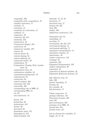

This document is the PhD thesis of Stéphane Lengrand from Université Paris VII and the University of St Andrews. The thesis contributes to extending the framework of the Curry-Howard correspondence to logics like sequent calculus that are well-suited for proof search, and to classical rather than just intuitionistic reasoning. The thesis has three parts. The first part develops proof terms for intuitionistic implication in natural deduction and sequent calculus, including normalization and cut-elimination. The second part builds a theory of pure type systems in sequent calculus. The third part studies approaches to classical type theory, developing a sequent calculus for a classical version of System Fω and discussing canonical forms


![[Slfm 118] theory of relations roland fraisse (nh 1986)(t)](https://cdn.slidesharecdn.com/ss_thumbnails/slfm118theoryofrelations-rolandfraissenh1986t-140808170208-phpapp01-thumbnail.jpg?width=640&height=640&fit=bounds)


