1. DETERMINING THE EFFECTS OF FRESH WATER RELEASES ON THE
MARITIME ENVIRONMENT, IMPLICATIONS FOR A MORE
SUSTAINABLE FUTURE
by Jonathan N. Valentine
Department of Geosciences, Universityof SouthFlorida, 4202 E Fowler Avenue,Tampa,FL 33620,USA; e-mail: Valentine5@mail.usf.edu
Introduction: Florida Geology and Water
Management
The Geology of Florida is dominated
not by rocks, but by water. As such, water
management is one of the state’s biggest
concerns. The management and utility of
water resources directly effects Florida’s
economy and the quality of life of its
citizens. With the advent of the global issue
of climate change, and increased
urbanization certain water management
techniques must be looked at through a
closer lens in order to limit possible
economic impacts as well as environmental
ones (Stanton 2007). One such management
technique that requires further review is the
practice of freshwater releases or
“Flushings” within the Caloosahatchee
Estuary.
In the Caloosahatchee estuary,
freshwater releases (FRs) occur
intermittently during times of high flood risk
in order to drain excess water stored in Lake
Okeechobee (Doering 1999). This excess
water is derived from water stored in over
115 km of levees and 800 km of canals in
southwest Florida that divert water from
wetlands for either water storage or flood
control (Finkl, 1995). Previous studies have
shown that the nutrient rich water that is
released from Lake Okeechobee into the
Caloosahatchee estuary via the
Caloosahatchee River has significant effects
on salinity and water quality, as well as
possible effects on turbidity and chlorophyll
a (Doering 1999), (Buzzelli 2014).
Furthermore, higher levels of marine and
macrobenthic diversity within the estuary is
believed to be directly related to low levels
of freshwater release (Palmer 2015).
Findings such as these influenced the
founding of the Estuaries Protection
program in 2007 (Section 373.4595, Florida
Statutes) which is responsible for
establishing minimum inflow levels within
the estuary (Sections 373.042 and 373.0421
of Florida Statutes).
However, establishing these inflow
levels is still an area of active research
within water management and the current
findings are limited in two ways. First, no
significant studies have provided any

2. quantification of the effects of freshwater
releases outside of the estuary into the
maritime environment. Second, the issue of
increased levels of urbanization and
flooding frequency have not been
adequately addressed in relation to how they
will affect the management of freshwater
releases in the future.
Introduction: The solution
In order to address the first issue, a
preliminary quantification of the effect of
freshwater releases over time in the
maritime environment can be inferred
through paleo-ecological study of modern
and past assemblages. Various diversity
indices and metrics have been shown to
quantify changes in specific assemblages
over time (Schipper et al 2016). These
methods have become increasingly
important as conservational techniques that
quantify anthropogenic impacts within
specific environments (Schipper et al 2016),
(Kidwell 2013). In the maritime
environment it is important to be able to
accurately compare dead communities with
their live counterparts, therefore molluscan
assemblages act as important
paleontological proxies as their hard body
parts are well preserved and they represent a
limited geologic range (Kidwell 1996).
Introduction: The study
In this study, the live-dead fidelity
and live-dead rank order abundance of
gastropod communities were analyzed from
dredge localities taken within two different
maritime zones outside of the
Caloosahatchee estuary. These two zones
represent areas that are either at high risk of
being influenced by freshwater releases or
areas that are at low risk of being
influenced. Dredge localities were deemed
to be either high risk or low risk based off
two factors, distance from the estuary and
the analysis of ocean current charts which
depict the movement of water from the
estuary into the maritime environment. The
areas deemed low risk act as the control
group within this study as it is unlikely that
these dredge localities are being influenced
by the freshwater releases, while the areas
deemed high risk will act as the
experimental group.
Furthermore, as it is commonly
accepted that global diversity is decreasing,
any change in fidelity or rank order
abundance across the control group will be
treated as background noise when being
compared to the experimental group
(Schipper et al 2016). Therefore, the
experimental group (High Risk) will have to
differ in some significant manner from any

3. discordances that occur in the control (low
risk) for conclusions to be drawn.
Furthermore, the relation between the effects
of freshwater releases to the issues of
urbanization, wetland reduction, and
increased flooding frequency due to climate
change are addressed within the discussion.
*editor’s note: Include statistics for
carnivore to non-carnivore ratios as well?
This could act as further supporting
evidence?
Methods: Materials
The Gastropod assemblages used in
this study were all acquired via dredges
taken by the research vessel R/V Bellows as
part of ongoing research in the Gulf of
Mexico by the Paleo-ecology Lab at USF
(Herbert 2016). Dredges were taken for 20
minute intervals and shell assemblages were
brought back to the lab to be processed. In
order to preserve live dead agreement and
remove taphonomic bias a sieve size above
1.5 mm was used (Kidwell 2002). The
gastropods were then divided into their
respective species, and then further
subdivided based on live or dead
classification.
Ocean Current data published by
PODAAC, an extension of Nasa’s Jet
propulsion laboratory, was used in order to
help classify 29 different dredge localities as
possible stations of interest (ESR 2009).
These dredge localities were then grouped
into eleven zones in order for each zone to
retain a large enough sample size to limit
taphonomic bias (Kidwell, 2001). The zones
were grouped based off their relative
distance between each other with a
maximum separation of eight miles in order
to meet a minimum threshold count of 45
live specimens. The zones were then
characterized based off of their total distance
from the mouth of the Caloosahatchee
estuary which is the parameter of interest as
it is the source of freshwater releases
(Doering 1999). Zones within 45 miles of
the mouth of the estuary were deemed high
risk for anthropogenic impact as these zones
were the most likely to come into contact
with excess freshwater released from lake
Okeechobee, conversely areas further from
this cutoff were deemed low risk. As such,
hypotheses concerning anthropogenic
impact focused on the possibility of
significant degradation to molluscan
communities in the high risk areas.
*editor’s note: (It is possible to superimpose
the Ocean current data on to google Earth,
this would make an incredibly useful figure
to show how I quantified which dredge
localities I used, currently it looks like I just

4. picked them at random, however that is not
true).
Methods: Quantitative Statistical
Analysis
These two different type localities,
high and low risk, were subsequently
analyzed via Live-dead fidelity analysis and
live-dead rank order abundance. Both
Metrics are used to quantify how closely the
live and dead communities within a given
locality approximate each other. The two
metrics approach this quantification by
different pathways, live-dead fidelity is
based on the total number of species both
live and dead while live-dead rank order
abundance is focused solely on the highest
ranking species based on abundance, in this
case the five highest ranking species in
abundance (Lockwood 2006).
Live-dead fidelity readings for each
zone were plotted as a function of distance
from the mouth of the Caloosahatchee
estuary. A linear regression was then
performed to infer a possible trend as well as
analyze statistical power.
Live-dead fidelity
The live dead fidelity metric is
calculated as follows:
𝐿𝑖𝑣𝑒 − 𝐷𝑒𝑎𝑑 𝐹𝑖𝑑𝑒𝑙𝑖𝑡𝑦 = (𝑁 𝑆 × 100)/(𝑁𝐿 + 𝑁 𝑆)
Where NS is equivalent “to the number
of species found in both the live community
and death assemblages”, and NL “is
equivalent to the number of species found in
the live community only” (Lockwood 2006).
This study is limited in regards to
calculating live dead fidelity as each
location is only a single snapshot of both the
live and the dead communities which limits
overall fidelity (Lockwood 2006). However,
the aim of this study is to quantify possible
anthropogenic effects of freshwater releases,
therefore a comparison of live-dead fidelity
between the high and low risk localities
should be sufficient enough to make relative
assumptions on environmental or
anthropogenic contributors.
In order to optimize the strength of a
live-dead fidelity study a threshold size of
100 individuals is optimal in order to
account for factors such as time averaging
and sample bias (Kidwell 2001). In this
study, live individuals were rare, therefore a
threshold size of 45 was set in order to make
inferences from the datasets currently
available. Furthermore, dredge localities
with similar coordinates were combined into
zones that were then able to meet the
minimum threshold requirement previously
set in this study. These “zones” are
represented by a single GPS coordinate that

5. was tabulated through an online calculator,
geomidpoint, that transformed all GPS
coordinates into Cartesian coordinates which
were then multiplied by a weighting factor
and added together to determine the best fit
location for the average of a given set of
GPS coordinates.
In order to interpret the results of this
study it is important to understand that a
perfect Live-dead fidelity would be
represented by a score of 50, while a score
of 100 would represent a community with
no live-dead fidelity. Examples for such
calculations are shown in figures 1 and 2.
𝐿𝑖𝑣𝑒 − 𝐷𝑒𝑎𝑑 𝐹𝑖𝑑𝑒𝑙𝑖𝑡𝑦 =
𝑁𝑆 × 100
𝑁𝐿 + 𝑁𝑆
=
40 × 100
0 + 40
= 100
𝐿𝑖𝑣𝑒 − 𝐷𝑒𝑎𝑑 𝐹𝑖𝑑𝑒𝑙𝑖𝑡𝑦 =
𝑁𝑆 × 100
𝑁𝐿 + 𝑁𝑆
=
40 × 100
40 + 40
= 50
Rank Order Abundance
Rank order abundance is used in ecology
to rank the most prominent species in a
given parameter by abundance (Kidwell
2001). In this study, the parameter under
study is gastropod diversity. Previous
studies involving Spearman Rank
Correlations have shown that rank order
abundance between live and dead molluscan
species in a pristine, unchanged environment
with a threshold size of 100 should correlate
significantly (Kidwell 2001, Lockwood
2006). Therefore, any strong deviations in
rank order abundance between live and dead
species of gastropod datasets suggests
possible environmental impacts within a
given locality. Due to time constraints, rank
order abundance was not calculated in this
draft, however given an extended deadline
this study can easily be edited to include
such statistical information.
Editor’s note* Quantitative or
qualitative representation of rank order
abundance data?
Results
The results in this experiment are
limited due to the fact that limited
abundances of live assemblages were
available to calculate live-dead fidelity.
Furthermore, only minor sampling efforts
have been undergone outside of the
Caloosahatchee Estuary, therefore the
amount of zones available for study were
further atrophied.
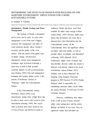
Figure 1: Live-dead fidelity calculation where
the total number ofspecies presentin both
live and dead assemblages,NS,is equal to
40, and the number of species presentin the
live assemblage,NL, is equal to 0. This
represents no fidelity.
Figure 2: Live-dead fidelity calculation where
the total number ofspecies presentin both live
and dead assemblages,NS, is equal to 40, and
the number ofspecies presentin the live
assemblage,NL,is equal to 40. This represents
perfect fidelity.

6. However, figure 3 does show a trend
line that exhibits an increase in live-dead
fidelity as the distance from the estuary is
increased. The figure plots the linear
regression of live dead fidelity for each zone
against the distance from the mouth of the
Caloosahatchee River which is the
parameter at interest as it is the source of
freshwater releases into the estuary.
The trend line could be an artifact of
variance, as the R2 value is distinctly low at
.029. This drastically decreases the power of
the study to make significant conclusions.
However, it does serve as the basis for
justifying further investigation into the
effects of freshwater releases in the maritime
environment. Table 1 represents the raw
data used to generate figure 3.
Discussion
The purpose of this study was to
investigate the possibility of freshwater
releases impacting the maritime
environment. However, due to constraints
on sample size, this study does not have the
power to make statistically significant
conclusions. However, the data does
highlight the possibility of freshwater
releases acting as a negative anthropogenic
factor on molluscan communities outside of
the estuary. As humans continue to impact
the natural environment in a myriad of
currently unquantified ways, it is important
to begin the quantifications of anthropogenic
factors in order to limit potential impacts
(Steffen W. et al. 2007). The data tabulated
in this study suggests that freshwater
releases are possibly negatively impacting
the maritime environment off of the
Caloosahatchee estuary.
Further research into this subject
could have far reaching applications as
issues such as urban development, tourism,
and climate change are prominent issues in
modern Florida politics. The current system
that Florida employs in draining water into
the gulf is a broken one. It was designed in
the early 20th century when environmental
issues were not yet a considerable notion
(Finkl, 1995). This ignorance has led to the
negative effects we currently see in the
Caloosahatchee estuary due to freshwater
releases (Doering 1999), (Buzzelli 2014). If
there is evidence that these effects extend
into the maritime environment, appropriate
steps must be taken in order to either limit or
negate any possible effects. The idea of
sustainability means planning for the future
while the problems still appear to be small
now.

7. Freshwater releases are currently a
strategy implemented to relieve strain from
large flooding events (Finkl 1995).
However, due to wetland reduction,
urbanization, and climate change it is
unclear if the releases will remain a viable
method in the future as flooding frequency
and strength will likely continue to rise.
In regards to wetland reduction, over
half of the wetlands across the world have
been lost while the remaining portion is
diminishing (Zedler 2005). Florida is no
exception to this and has seen a continued
decrease of wetlands over recent years
(Dahl, 2005). Wetlands play a key role in
diminishing flooding events as they act as
natural flood mitigation devices (Brody
2007), (Ming 2007).
In regards to urbanization, Florida has
been experiencing rapid population growth
and with that growth the conversion of
natural resources once used for forestry,
agriculture, or even open space always
occurs (Reynolds 2001). In order to limit
wetland reduction and decrease flooding
events it is pivotal that plans for future
development take into account wetland
reduction, as there exists a rollover effect on
countless environmental systems including
freshwater releases when Florida’s wetlands
are destroyed due to urbanization (Brody
2007).
Finally, in regards to climate change,
accelerated sea live rise due to increases in
global temperature means will play a large
role in how freshwater releases are
managed. In Florida, there has already been
a significant increase in flooding frequency
as related to sea level rise (Wdowinski
2016). Furthermore, this trend is expected to
increase dramatically over the next fifty
years (Wdowinski 2016).
These factors unanimously point to there
likely being a dramatic increase in the
amount of water that needs to be drained
through the Caloosahatchee River in the
upcoming years if the current method of
flood mitigations is not revamped. In failing
to do so, some of Florida’s natural systems
could be irrevocably damaged. Furthermore,
failing to act could damage large amounts of
Florida’s aesthetic value, damaging the
tourism industry, a crucial aspect of
Florida’s economy (Stanton 2007).
There exists a multitude of
environmental controls in place across the
world that have important functions yet their
contributions toward sustainability remain at
a minimum. These systems need to be
constantly evaluated and if necessary

8. completely restructured if doing so will have
long term benefits. Keeping this in mind it is
important to continue research into the
effects of freshwater releases as it may
already be necessary to reevaluate current
water management techniques where these
releases are concerned
References
Brody, S. D.,et al. (2007). "The rising costs of
floods: Examining the impact of
planning and development decisions on
property damage in Florida." Journal of
the American Planning Association
73(3): 330-345.
Buzzelli, C., et al. (2014). "Fine-scale detection
of estuarine water quality with managed
freshwater releases."Estuaries and
coasts 37(5):1134-1144
Dahl, T. E. (2005). "Status and trends of
wetlands in the conterminous United
States 1998 to 2004."
Doering, P. H. and R. H. Chamberlain (1999).
WATER QUALITY AND SOURCE
OF FRESHWATER DISCHARGE TO
THE CALOOSAHATCHEE
ESTUARY,FLORIDA1,Wiley Online
Library.
ESR. 2009. OSCAR third degree resolution
ocean surface currents. Ver. 1.
PO.DAAC,CA,USA. Dataset accessed
[YYYY-MM-DD].
Finkl, C. W. (1995). "Water resource
management in the Florida Everglades:
Are'lessons from experience'a prognosis
for conservation in the future?" Journal
of Soil and Water Conservation 50(6):
592-600.1
Kidwell, S. M. and K. W. Flessa (1996). "The
quality of the fossil record: populations,
species, and communities 1." Annual
Review of Earth and Planetary Sciences
24(1): 433-464.
Kidwell, S. M. (2001). "Preservation of species
abundance in marine death
assemblages." Science 294(5544): 1091-
1094.
Kidwell, S. M., et al. (2001). "Sensitivity of
taphonomic signatures to sample size,
sieve size, damage scoring system, and
target taxa." Palaios 16(1):26-52.
Kidwell, S. M. (2002). "Mesh-size effects on the
ecological fidelity of death assemblages:
a meta-analysis of molluscan live–dead
studies." Geobios 35:107-119.
Kidwell, S. M. (2013). "Time‐averaging and
fidelity of modern death assemblages:
building a taphonomic foundation for
conservation palaeobiology."
Palaeontology 56(3):487-522.
Lockwood, R. and L. R. Chastant (2006).
"Quantifying taphonomic bias of
compositional fidelity, species richness,
and rank abundance in molluscan death
assemblages from the upper Chesapeake
Bay." Palaios 21(4): 376-383.
Ming, J., et al. (2007). "Flood mitigation benefit
of wetland soil—A case study in
Momoge National Nature Reserve in
China." Ecological Economics 61(2):
217-223.
Palmer, T. A., et al. (2015). "Determining the
effects of freshwater inflow on benthic
macrofauna in the Caloosahatchee
Estuary, Florida." Integrated
environmental assessment and
management.
Reynolds, J. E. (2001). Urbanization and land
use change in Florida and the South.
Current issues associated with land
values and land use planning.
Proceedings of a regional workshop.
Southern Rural Development Center,
Mississippi State,MS.

9. Schipper, A. M., et al. (2016). "Contrasting
changes in the abundance and diversity
of North American bird assemblages
from 1971 to 2010." Global Change
Biology.
Steffen, W., et al. (2007). "The Anthropocene:
are humans now overwhelming the great
forces of nature." AMBIO: A Journal of
the Human Environment 36(8):614-
621.
Stanton, E. A. and F. Ackerman (2007). "Florida
and climate change: the costs of
inaction." Florida and climate change:
the costs of inaction.
Wdowinski, S., et al. (2016). "Increasing
flooding hazard in coastal communities
due to rising sea level: Case study of
Miami Beach,Florida." Ocean &
Coastal Management 126:1-8.
Zedler, J. B. and S. Kercher (2005). "Wetland
resources:status, trends, ecosystem
services, and restorability." Annu. Rev.
Environ. Resour. 30:39-74.
Table 1: All data generated in this table is taken from raw dredge data that was
collected on a series of research cruises by the R.V. Bellows in the Gulf of
Mexico

10. Zone NS NL Live-Dead
Fidelity
Dead
Count
Live
count
Distance from
Mouth of
Caloosahatchee
River (miles)
GPS coordinate
(avg)
Zone 1 (XVIIIK, VA)
32 16 66.6666667
110 436 13.5 26.460246
-82.210423
Zone 2 (IIIABC,
XVIIIQ)
30 16 65.2173913
280 46 35 26.011126
-82.034434
Zone 3 (IIIED,
XVIIIOP)
61 20 75.308642
297 55 40.77 26.17662
-82.536033
Zone 4 (VIIIAB)
30 14 68.1818182
230 59 55.15 25.759784
-81.715175
Zone 5(VIIICD)
18 14 56.25
74 45 54.8 25.751842
-81.781733
Zone 6 (VIIIE)
13 8 61.9047619
80 45 54.27 25.75016667
-81.83233333
Zone 7 (IXABC)
32 22 59.2592593
374 112 78.68 25.498651
-81.438209
Zone 8 (IXD)
16 10 61.5384615
200 114 73.35 25.4998
-81.66963333
Zone 9 (IXE)
25 11 69.4444444
228 87 71.59 25.49921667
-81.77748333
Zone 10 (XAB, XIA)
36 16 69.2307692
247 64 90 25.361216
-81.323684
Zone 11 XCDEF, XIDE
46 25 64.7887324
249 116 83.5 25.363304
-81.594675

11. Figure 3: Linear regression of live-dead fidelity and
distance from the Caloosahatchee Estuary and
Google earth coordinates with each zone shown.