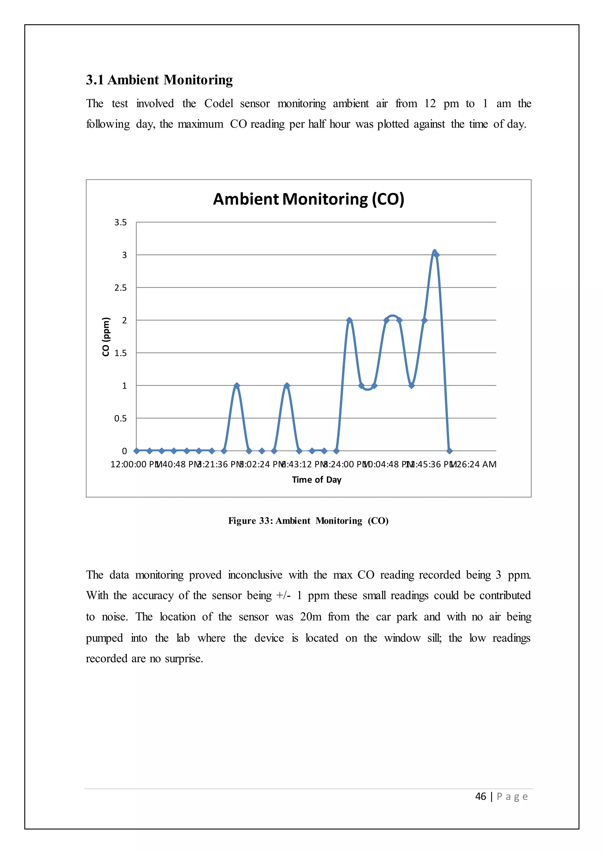
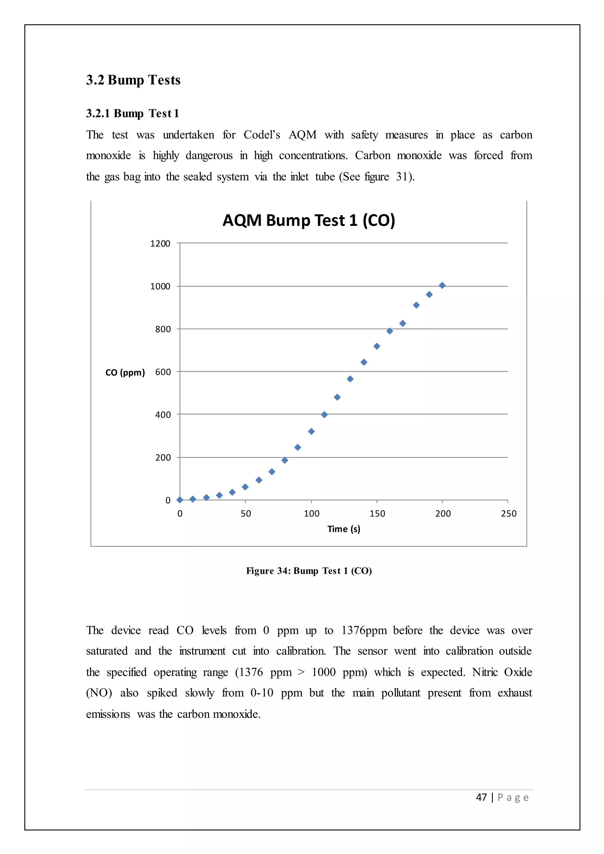
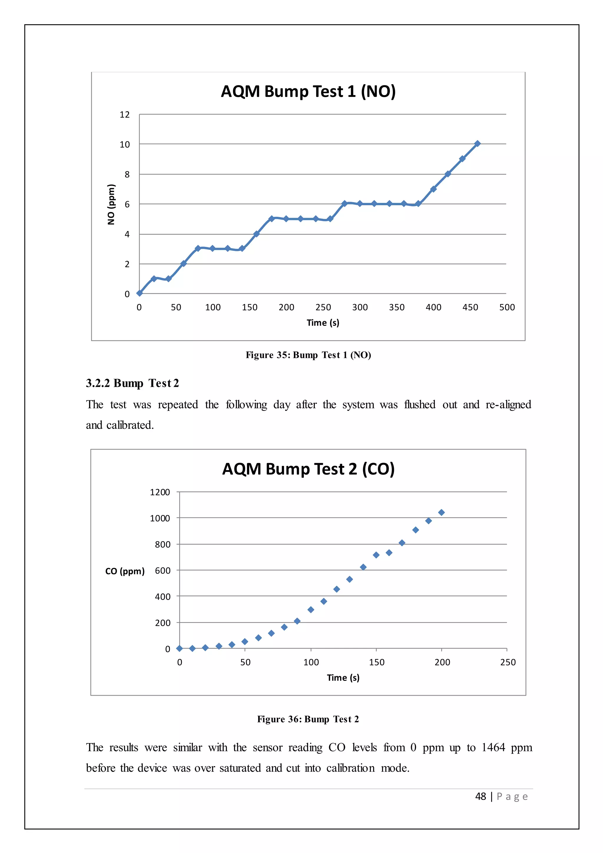
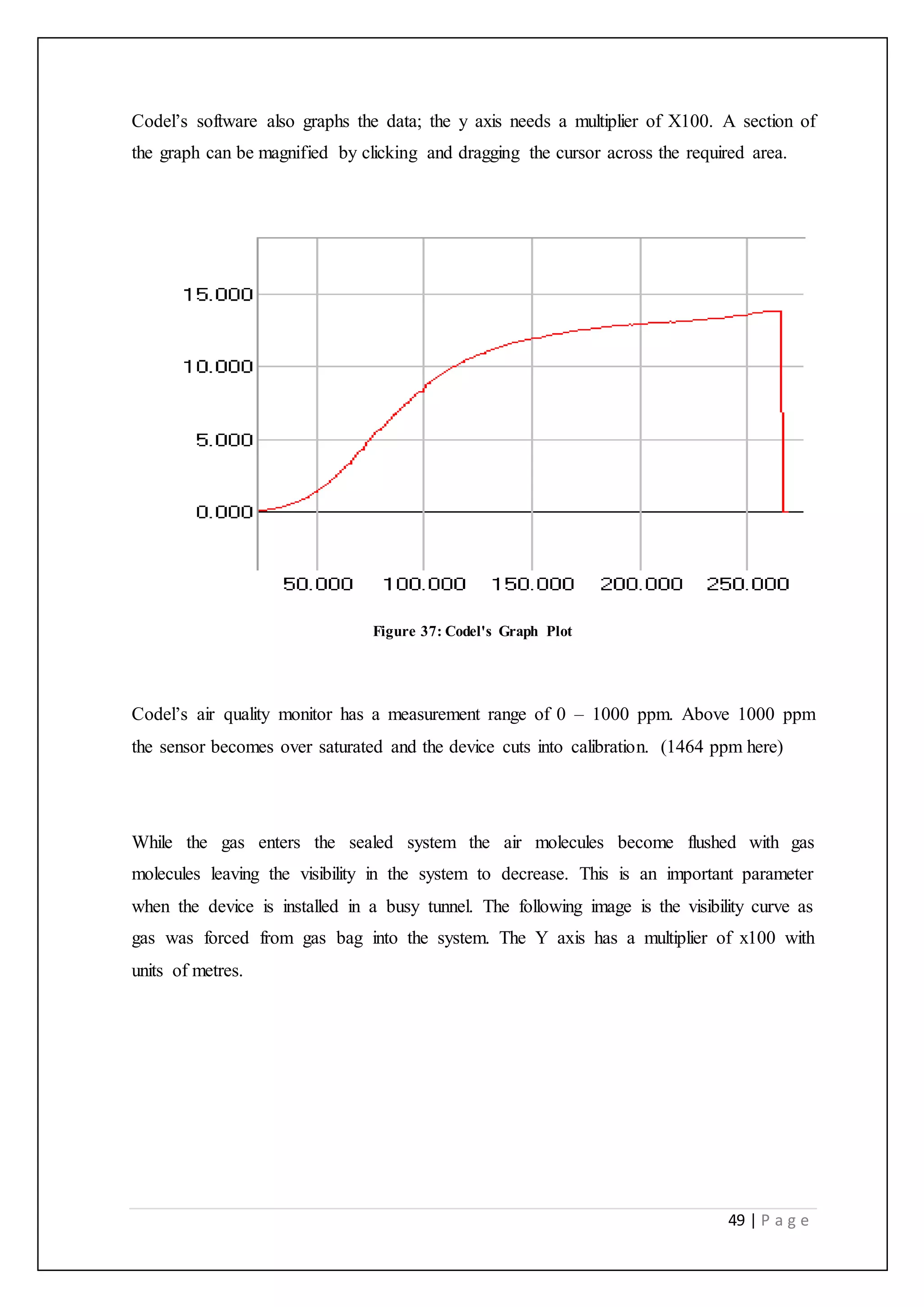
The document describes the commissioning of a Codel Tunnel Craft 3 air quality monitor. The device measures carbon monoxide, nitric oxide, and visibility in tunnels. It was taken out of service from the Jack Lynch Tunnel and re-commissioned by wiring and calibrating it. Testing showed good correlation between the Codel sensor and a separate carbon monoxide probe, proving the sensor was accurately re-commissioned and ready for reinstallation.

1. Commissioning and Testing of a CODEL Tunnel Craft Air
Quality Monitor
By
Richard Duffy
Department of Applied Physics and Instrumentation,
Cork Institute of Technology
Abstract
Codel’s Tunnel Craft 3 is a tunnel monitoring device made in the UK and is deployed in
many tunnels worldwide for monitoring of carbon monoxide, nitric oxide and visibility.
The project entails re-commissioning the device back to working order for installation. The
device was wired and calibrated. A bump test was undertaken to check that the sensor was
recording CO, NO & Visibility. A comparison of carbon monoxide recorded for Codel’s
sensor compared with an Alpha sense probe was undertaken and the data had very good
correlation which proves the sensor is re-commissioned and ready for permanent
installation.
Submitted in partial fulfilment of the regulations for a Bachelor of Science (Honours)
In
Environmental Science & Sustainable Technology
February 2015

2. 1 | P a g e
Declaration
I hereby certify that this material, which I now submit for assessment is entirely my own
work and has not been taken from the work of others save and to the extent that such work
has been cited and acknowledged within the text of the report.
____________
Richard Duffy

3. 2 | P a g e
Table of Contents
Contents
List of Figures.......................................................................................................................... 5
Acknowledgements .................................................................................................................. 6
Introduction ............................................................................................................................. 7
1.1 Background............................................................................................................... 8
1.2 Gas Detection Methods .............................................................................................. 8
1.2.1 Electrochemical.................................................................................................. 8
1.2.2 Infrared.............................................................................................................. 9
1.2.3 Semiconductor ................................................................................................... 9
1.2.4 Ultrasonic .......................................................................................................... 9
1.3 A Comparison of CODEL sensors and alternative Manufacturers ................................10
1.3.1 Key Design Parameters............................................................................................10
1.3.2 Path Length.............................................................................................................10
1.3.3 Choice of Infrared Detector ......................................................................................10
1.3.4 Measurement of NO.................................................................................................11
1.4 Theory.....................................................................................................................11
1.4.1 The Tunnel Craft 3 Concept...............................................................................11
1.4.2 What gases are measured and why?....................................................................11
1.4.3 CO, NO and Visibility Air Quality Monitor ........................................................12
1.4.4 Absorption of light...................................................................................................14
1.4.5 Absorption spectrum of CO......................................................................................14
1.4.6 Beer-Lambert Law...................................................................................................15
1.5 Equipment................................................................................................................15
1.5.1 Power Supply Unit (PSU)............................................................................................15
1.5.2 Station Control Unit (SCU)..........................................................................................16
1.5.3 WinCom Software.......................................................................................................17
1.6 Principles of Operation...................................................................................................18
1.6.1 Air Quality Monitor.....................................................................................................18
1.6.1.1 Visibility Measurement .........................................................................................18
1.6.1.2 Measurement Elements..........................................................................................19
1.6.1.3 LED Control.........................................................................................................19
1.6.1.4 Detector Element ..................................................................................................19

4. 3 | P a g e
1.6.1.5 Diagnostic Data ....................................................................................................20
1.6.1.6 Calibration............................................................................................................21
1.6.2 CO & NO Measurement ..............................................................................................21
1.6.2.1 Gas Cell Correlation..............................................................................................21
1.6.2.2 Measurement Elements..........................................................................................22
1.6.2.3 Detector Operation................................................................................................22
1.6.2.4 Stepper Motor Control...........................................................................................22
1.6.2.5 Integration of CO/NO & Visibility Measurements...................................................22
1.6.2.6 Calibration............................................................................................................23
1.7 Technical Specifications .................................................................................................23
1.7.1 General...................................................................................................................23
1.7.2 Sensor Unit .............................................................................................................23
1.7.3 Power Supply Unit...................................................................................................24
1.8 Device Wiring ...............................................................................................................24
1.8.1 Wiring Power Supply Unit...........................................................................................24
1.8.2 Wiring Station Control Unit .........................................................................................25
1.8.3 Set Sensor Addresses...................................................................................................27
1.8.4 Wiring Air Quality Monitor...........................................................................................28
1.8.5 Commissioning ...........................................................................................................28
1.8.5.1 Power up (SCU)....................................................................................................28
1.9 Installation.....................................................................................................................29
1.9.1 Mounting AQM.......................................................................................................29
1.9.2 Alignment of AQM Sensor.......................................................................................29
Experimental Setup .................................................................................................................30
2.1 Wiring the Device..........................................................................................................31
2.1.1Wiring the RS232 Communications...............................................................................33
2.2 Software Configuration ..................................................................................................34
2.2.1 Alignment...................................................................................................................34
2.2.2 Detector Levels...........................................................................................................36
2.2.3 Thermistor Control......................................................................................................37
2.2.4 Output............................................................................................................................38
2.2.4.1 Instantaneous v Smoothed measurement ........................................................................39
2.2.5 Y-Values........................................................................................................................39
2.2.6 Calibration......................................................................................................................40

5. 4 | P a g e
2.3 Testing ..........................................................................................................................41
2.3.1 Overnight data recording .............................................................................................41
2.3.2 Bump Test..................................................................................................................42
2.3.3 Cross Calibration Test .................................................................................................43
2.3.4 Technical Specs for Carbon Monoxide Alpha Sense Probe.............................................44
Analysis of Results..................................................................................................................45
3.1 Ambient Monitoring.......................................................................................................46
3.2 Bump Tests ...................................................................................................................47
3.2.1 Bump Test 1 ...............................................................................................................47
3.2.2 Bump Test 2 ...............................................................................................................48
3.3 Cross Calibration Test....................................................................................................51
3.4 Report Generation..........................................................................................................52
Concluding Remarks ...............................................................................................................53
4.1 Discussion .....................................................................................................................54
4.2 Future Work ..................................................................................................................54
4.3 Conclusion ....................................................................................................................54
References..............................................................................................................................56

6. 5 | P a g e
List of Figures
Figure 1: CO Exposure Effects ................................................................................................12
Figure 2: AQM Transceiver .....................................................................................................13
Figure 3: Infrared and Visible light channels .............................................................................13
Figure 4: Reflector ..................................................................................................................14
Figure 5: CO Absorption Spectrum...........................................................................................15
Figure 6: Power Supply Unit ...................................................................................................16
Figure 7: Station Control Unit .................................................................................................17
Figure 8: General Screen Characteristics ..................................................................................18
Figure 9: Silicon photo-detector ..............................................................................................20
Figure 10: Power Supply Unit .................................................................................................24
Figure 11: Station Control Unit Schematic ...............................................................................25
Figure 12: Wiring of Station Control Unit .................................................................................26
Figure 13: SCU Address Switches............................................................................................27
Figure 14: AQM Sensor Switch................................................................................................27
Figure 15: Air Quality Monitor Wiring .....................................................................................28
Figure 16: Device Wired..........................................................................................................31
Figure 17: AQM Wired............................................................................................................32
Figure 18: RS232 Female Pin out ............................................................................................33
Figure 19: RS232 Soldered Connection ....................................................................................33
Figure 20: Detector Aligned.....................................................................................................34
Figure 21: Saturated Detector...................................................................................................35
Figure 22: Detector Misalignment ............................................................................................35
Figure 23: Detector Levels Range ............................................................................................36
Figure 24: Detector Level Saturated..........................................................................................36
Figure 25: Thermistor Control..................................................................................................37
Figure 26: Output Configuration...............................................................................................38
Figure 27: Y-Values ................................................................................................................39
Figure 28: Stop Calibration ......................................................................................................40
Figure 29: CO Overnight Recording .........................................................................................41
Figure 30: Visibility Overnight Recording ................................................................................41
Figure 31: Experimental Set-Up ...............................................................................................42
Figure 32: Cross-Calibration Test.............................................................................................43
Figure 33: Ambient Monitoring (CO) .......................................................................................46
Figure 34: Bump Test 1 (CO)...................................................................................................47
Figure 35: Bump Test 1 (NO)...................................................................................................48
Figure 36: Bump Test 2 ...........................................................................................................48
Figure 37: Codel's Graph Plot...................................................................................................49
Figure 38: Visibility Graph ......................................................................................................50
Figure 39: Cross Calibration Test .............................................................................................51
Figure 40: Report Generation ...................................................................................................52

7. 6 | P a g e
Acknowledgements
Firstly I would like to thank Dr Josh Reynolds for his support and guidance throughout the
duration of the project. His enthusiasm and approachability made it a pleasure to have him
as my supervisor. To Dr Guillaume Huyet, who supported us all year and gave us great
advice to achieve our goals. Thanks to the senior lab technician Stephen Collins for his
advice and support on the project. Also my family and friends who help keep me motivated
with their invaluable support.

8. 7 | P a g e
Chapter 1
Introduction

9. 8 | P a g e
1.1 Background
Codel International Ltd is a UK company based in Bakewell, Derbyshire. The company
specialises in the design and manufacture of high-technology instrumentation for the
monitoring of combustion processed and atmospheric pollutant emissions. The Tunnel
Craft 3 Air Quality Monitor (AQM) is the industry proven tunnel atmosphere sensor [1].
The device is a single compact sensor which can measure CO, NO and visibility. It consist
of a transceiver that projects visible and infrared beams to a reflector mounted 3 m away.
The reflector reflects the light back to the transceiver and the specific absorption is
measured to determine the visibility coefficient, carbon monoxide and nitric oxide
concentration within the path of the beams.
In the past 15 years Codel tunnel sensors have been used in more than 400 road and rail
tunnels around the world. Some well-known destinations include Eurotunnel France, Lane
Cove tunnel in Australia and SMART tunnel in Malaysia. Codel is without doubt the world
leader in tunnel atmosphere monitoring [1].
This project deals with the commissioning and testing of a Codel Tunnel Craft 3 air quality
monitor. The instrument was up to quite recently deployed in the Jack Lynch Tunnel in
Cork and the initial objective is to get the equipment back to operational status. Further
requirements include calibrating the device and to critically compare it with other available
tunnel gas detectors.
1.2 Gas DetectionMethods
As technology has evolved so have the methods for detecting gas concentrations. The first
carbon monoxide detector was a simple white pad which would get stained if CO was
present. Newer models have alarms, flashing lights and can be programmed to go on/off
once a certain concentration has been present. Gas detectors can be portable or fixed, fixed
detectors can usually monitor more than one gas at a time. They can be classified
according to the following operation mechanisms:
1.2.1 Electrochemical
These detectors have a porous membrane which the gas will diffuse through to an
electrode. Here the gas will be chemically oxidized or reduced. The concentration of gas

10. 9 | P a g e
present relates to the current produced here [2]. The manufacture can alter the barrier to
detect certain gas concentration ranges. The physical barrier makes the device stable and
reliable with low maintenance. However the life span is 1-2 years due to corrosive
elements [3]. These detectors are widely used in industry such as gas turbines, chemical
plants etc.
1.2.2 Infrared
Infrared sensors work by the principle of specific absorption at certain wavelengths. They
use radiation which passes through a known volume of gas. For example, CO absorbs
wavelengths of about 4.2-4.5 μm [4]. The energy present in this range is compared to a
wavelength outside the range; the difference in energy present is the concentration of gas
present [4]. A major advantage is the remote sensing capabilities of an infrared sensor; it
does not have to be in contact with the gas to detect it. This allows large volumes of space
to be monitored. This is one reason Codel uses infrared for monitoring inside tunnels.
Another advantage for tunnel application is its ability to detect high levels of carbon
monoxide from vehicles [4].
1.2.3 Semiconductor
This sensor uses chemical reactions to detect the presence of gases when it comes in
contact with the sensor. The electrical resistance in the sensor decreases when it comes in
contact with the gas. This change is resistance is used to calculate the gas concentration
present. Semiconductors are commonly used for detection of carbon monoxide but the
downfall of this technique is the sensor must come in contact with the gas and therefore
works over a much shorter distance than infrared detectors [5]. This is why semiconductor
sensors are generally not used in tunnel applications.
1.2.4 Ultrasonic
Ultrasonic gas detectors detect changes in background noise in the local environment by
acoustic sensors. This system is generally used to detect gas leaks; high pressure leaks will
produce sound in the ultrasonic range. This is distinguished from the background acoustic
noise. They cannot measure concentration so are not used in tunnel applications [6].

11. 10 | P a g e
1.3 A Comparisonof CODELsensors andalternative Manufacturers
1.3.1 Key DesignParameters
Codel uses open path optical absorption technology. This has proved to be reliable and
highly accurate. However for optimum results a few key parameters must be met.
1.3.2 Path Length
The longer the path length the more gas is being measured, however this does not mean it
will produce more accurate data. An open path measurement system uses an optical
arrangement where a large broader beam is used to null the impact of optical
misalignment. The amount of energy received by the sensor reduces with the square of the
path length. This reduces the signal noise as the path length is increased. So we have two
conflicting parameters that decide the overall accuracy of an open path measurement
system. The measurement sensitivity increases with path length, while signal noise reduces
with the square of the path length. Both improve the signal noise ratio for the device. Codel
solution to this problem is to choose the shortest path length consistent with achieving the
required measurement sensitivity.
Codel Tunnel Craft 3 measures CO, NO and visibility over a path length of 6 metres, 3 m
from the transceiver to the reflector and vice versa. This ensures all three measurement
channels high accuracy will be comfortably satisfied. Other manufacturer’s sensors require
longer path lengths such as ten metres to achieve their specified accuracy [7]. This will
cause increased measurement noise. This is one major disadvantage of other products on
the market. A further disadvantage of long optical path length is it is unrealistic to maintain
accuracy over a wide measurement range when using a long path length. The Codel sensor
has the ability to maintain its accuracy over the full operating range of 0 to 300 ppm [7].
1.3.3 Choice of Infrared Detector
Codel uses a high quality thermo-electrically cooled lead selenide detector to achieve the
required sensitivity. For the 3 metre folded beam path it can maintain its accuracy for CO
measurement of 1 ppm for the range of 0-300 ppm. In comparison to other competitors

12. 11 | P a g e
sensors which use less high tech and cheaper pyroelectric detectors, having an accuracy
spec of only 5 ppm over a 10 metre path for the range 0-150 ppm [7].
1.3.4 Measurement of NO
Codel’s use of the lead selenide detector enables them to integrate a measurement channel
for NO into the tunnel sensor; this is not possible with other manufacturer’s pyroelectric
detectors. Codel sensors are unique in their ability to provide three key measurements (CO,
NO, Visibility) in the one sensor [7].
1.4 Theory
1.4.1 The Tunnel Craft 3 Concept
The device is designed exclusively for road tunnel applications. It can monitor carbon
monoxide, nitric oxide and visibility. Operating costs are at a minimum with the sensor
design having only one moving component and routine maintenance is simply cleaning of
the optical lens. There is also minimum tunnel cabling used and low installation costs.
Remote access of the diagnostic data and calibration input commands simplifies and
reduces the need for tunnel access.
1.4.2 What gases are measured and why?
Tunnel monitoring is extremely important for the health of its users as there is a risk to life
due to the gases involved. The combustion process along with exhaust fumes provides a
range of harmful toxic substances. The main players are carbon monoxide and nitric oxide.
Visibility is also a key issue for tunnel monitoring. Visibility is a measure of the distance at
which an object or light can be clearly distinguished. Vehicles release many gases which
can give a fog affect which in turn reduces visibility. In the still air of a tunnel environment
with little wind, a build-up of gases could be very detrimental to the visibility of the
drivers. Carbon monoxide and nitric oxide is a product of internal combustion engines, if
high levels are present these gases can easily cause fatal injuries. CO is non-smelling and
uncoloured at room temperature. It replaces O2 molecules in haemoglobin causing
suffocation. Therefore it is very important to continuously monitor, ventilate and if needed
raise an alarm when the prescribed limits are breached in the tunnel air.

13. 12 | P a g e
The acute effects produced by carbon monoxide in relation to ambient concentration in
parts per million are listed below:
Figure 1: CO Exposure Effects [1]
Gas detecting levels are generally drawn up in consultation with medical experts; however
the connection between gas concentrations and toxicity depends on many factors for each
tunnel. This makes it difficult to define exact limits for gas detection as each tunnel is an
individual case [8]. In comparison with ambient air, tunnel air is more stable as there is not
as much wind present. Wind can dilute pollution rapidly and disperse the pollution
concentration. This increases the need for low levels pollution in the tunnel environment.
In summary the three parameters stated are the main safety concerns in a road tunnel and
the Tunnel Craft 3 can monitor and detect them with high accuracy using the one sensor.
1.4.3 CO, NO and Visibility Air Quality Monitor
The AQM uses both infrared and visible light channels to measure visibility, carbon
monoxide and nitric oxide. The system consists of a transceiver that projects visible and
infrared beams to a reflector mounted 3 m away.

14. 13 | P a g e
Figure 2: AQM Transceiver
Figure 1 shows the transceiver that projects the visible and infrared light to the reflector.
Figure 3: Infrared and Visible light channels
Figure 2 shows the infrared and visible light channels. The reflector which is mounted 3m
away reflects the light back toward the transceiver (See Figure 3).

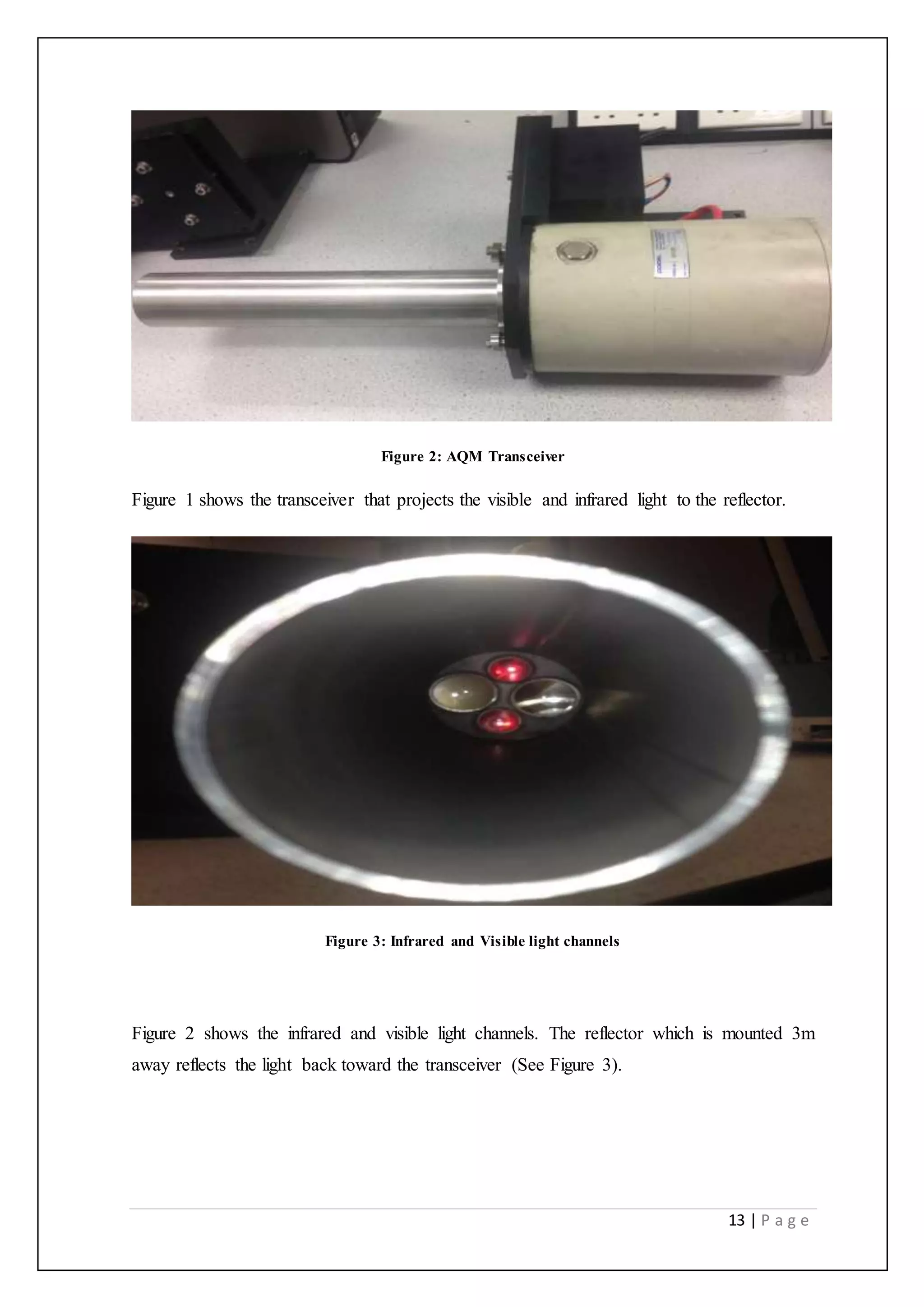
15. 14 | P a g e
Figure 4: Reflector
The specific absorption is measured to determine the visibility, CO /NO concentrations
within the path of the beam. A high powered LED is used for visible light source (See
Figure 2) while an infrared thermal source provides the infrared energy (See Figure 2). A
silicon photo-detector is used to measure the optical visibility; it determines the attenuation
of the light beam along the instruments sight path due the particulates present in the tunnel
atmosphere (See 1.6.1.4). The carbon monoxide and nitric oxide are measured using gas
cell correlation technology; it investigates the infrared absorption due to the presence of
CO and No in the instrument sight path (See 1.6.2.1). This provides a measurement for
atmosphere concentration in ppm.
1.4.4 Absorption of light
The absorption of light reduces the transmission of light as the atoms/molecules take up the
energy of a photon of light. Therefore due to the gases present in the tunnel, the reduction
of transmitted light is exponentially related to the concentration of the gas and the path
length of light travelled. In this case the path length is about 6m (distance from transceiver
to reflector * 2) [1].
1.4.5 Absorption spectrum of CO
‘’An absorption spectrum occurs when light passes through a cold, dilute gas and atoms in
the gas absorb at characteristic frequencies; since the re-emitted light is unlikely to be
emitted in the same direction as the absorbed photon, this gives rise to dark lines (absence
of light) in the spectrum’’ [9].

16. 15 | P a g e
The absorption of light reduces the transmission of light as the atoms/molecules take up the
energy. The IR spectrum of carbon monoxide has a major absorption band at 2100 cm-1 or
4.8 µm. The second absorption band seen below is carbon dioxide (CO2) whose absorption
band ranges from 2000- 2400 cm-1. Nitric Oxide has a major absorption band at 1886
cm1 or 5.3 µm.
Figure 5: CO Absorption Spectrum [10]
1.4.6 Beer-Lambert Law
Beer-Lambert Law relates the transmittance of light to absorbance by taking the negative
logarithmic function, base 10, of the transmittance observed by a sample, which results in a
linear relationship to the intensity of the absorbing species and the distance travelled by
light [4].
Absorbance = 2 - Log10 (T)
In summary, the law states that the absorbance is directly proportional to the concentration
of the sample and the path length [1].
1.5 Equipment
1.5.1 Power Supply Unit (PSU)
The power supply unit converts the mains supply to the 12v or 24v DC required to power
the air quality monitor.

17. 16 | P a g e
Figure 6: Power Supply Unit [1]
1.5.2 Station Control Unit (SCU)
The station control unit provides 48v dc power for the sensors on its local data bus. The
power supply unit provides the power input to the SCU. A local data bus links the SCU to
the sensor. The bus has two serial communication lines, MOSI (master out slave in) and
MISO (master in slave out). Master/Slave is a model for communication where one device
has control over other devices. The role of the station control unit is to access data from the
sensors to provide analogue and digital outputs. This data can be obtained via the RS232
serial port located inside the station control unit. WinCom software can be used to
communicate with the station control unit [1].

18. 17 | P a g e
Figure 7: Station Control Unit [1]
Description of the cards from right to left:
 RS232 connection- this communicates data from the AQM sensor to the laptop
 Relay output card- the relays can act as switches or as amplifiers ( converting small
current to larger)
 Current outputs- provides mA outputs
 Master micro- card contains microprocessor and software control
 Slave Micro- card contains microprocessor and software control
 Power supply card- includes 10 watts DC-DC converter
 Communications card- includes communications to SCU and CDC
1.5.3 WinCom Software
This is the software to be used to communicate the data from the RS232 port in the station
control unit to the user’s laptop. It enables all system data and controls to be accessed from

19. 18 | P a g e
the laptop. This software package can log data and graph it on the computer screen. Further
exploration of the software and its capabilities will be done at time of implementation and
testing.
Figure 8: General Screen Characteristics [1]
We can see above (figure 7) Codel’s WinCom software screen set up.
1.6 Principles of Operation
1.6.1 Air Quality Monitor
1.6.1.1 Visibility Measurement
This method of presenting this data is in the form of meteorological visibility. This is
defined as the distance over which the intensity of transmitted light falls to 5% of its initial
value. It represents the distance over which a person can see in a hazy or dusty
environment. I/Io is the ratio of the measured beam intensity and that of the initial intensity
Io and is known as the transmissivity (T) of the system.
In this case, I = 0.05 x Io thus T = 0.05

20. 19 | P a g e
And since k = 1/L * log e 1/T
Visibility L = 1/K log e 20 = 2.99/K
Where k is a parameter known as the visibility coefficient and is proportional to the
concentration of the suspended particles and L is the path length of the beam.
Thus, for a k value of 0.003, the visibility in metres is 2.99/0.003 = 1000m.
Both k factor and visibility are calculated by the sensor and are available for output [1].
1.6.1.2 Measurement Elements
A pulsed LED produces a beam of light focused by a lens to the reflector. The reflector has
an internal detector which monitors the brightness of the pulses of light. The beam
reflected is gathered by a second lens and focussed onto a receiving detector. The ratio of
signals of the two detectors provides the measurement of transmissivity. Transmittance is
the fraction of incident light at specific wavelength which passes through a sample, in this
case which is air.
1.6.1.3 LED Control
The LED emitting operation is controlled by an on board processor. A series of light pulses
is applied to the LED 4 times a second. Each pulse is extremely short in duration and the
pulse stream consists of approx. 100 pulses. The very brief nature of these pulses allows
the device to operate without interference from other light sources within the tunnel.
1.6.1.4 Detector Element
The initial brightness of the emitted light (Vis Tx) is measured by a silicon detector, while
another detector measures the intensity of the received light (Vis Rx) after transmission to
and reflection from the reflector.

21. 20 | P a g e
Figure 9: Silicon photo-detector [9]
The photo-detector contains pin photodiodes that utilize the photovoltaic effect to convert
optical power into an electrical current.
To monitor the background levels of light intensity the processor takes measurements prior
to pulsing the emitter LED. Then a series of measurements is taken with the LED on and
another series of measurements when it’s turned off to check the background levels
haven’t changed. This process occurs at high frequency which reduces the effects of any
background lighting [11].
1.6.1.5 Diagnostic Data
From the two detector measurements the transmissivity and opacity are calculated. Opacity
is a direct reading of the attenuation of light .It is a measure of the impenetrability. Zero
opacity equated to a totally clean light path and 100% to total light attenuation.
The measurement of opacity relies on having clean optical sources. If the surfaces of the
lenses or reflector become contaminated there will be a reduction in intensity of received
light and therefore an increase in opacity value. Over long periods of time this build-up of
contamination of lenses would result in a steady increase in opacity value. This appears as
a positive output drift. To fix this problem the optical surfaces should be cleaned regularly,
this could be a problem in a road tunnel but for this commissioning project it is a simple
but effective solution.

22. 21 | P a g e
1.6.1.6 Calibration
Normal procedures would all for calibration during a tunnel closure when it is expected
that the opacity value will be zero. The instrument can also be calibrated by selecting a
calibrate mode, where an opacity value of zero is assumed and the relevant calibration
factor is calculated:
Set Cal Vis = 10000 x Vis Tx/Vis Rx
Where Vis Tx is visibility transmitted from the transceiver and Vis Rx is visibility received
from the reflector.
1.6.2 CO & NO Measurement
Both Carbon Monoxide and Nitric Oxide absorb infrared energy. Both spectra behave like
a typical diatomic gas. They are made up of a number of fine absorption bands. Carbon
monoxide is fixed on a wavelength of 4.7 µm and Nitric Oxide 5.3 µm. This spectrum
allows gas cell correlation to take place in the analysis to determine the concentrations of
gases present.
The ratio of measurement of attenuation of infrared beam with and without a high
concentration of sample gas being measured allows us to derive a function which is
dependent solely on the concentration of gas to be measured. The advantage of this
technique is it uses a sample of the gas itself as a filter so it has extremely high immunity
to other interfering gases.
1.6.2.1 Gas Cell Correlation
This technique is ideal for a tunnel monitoring system as it is built to detect low level
measurements. It also has the ability to operate where there are background gases present
which could interfere with the measurement. The sensing mechanism is based on the
absorption principle where the gas can absorb unique light wavelengths. The principle is
simple, light travels through the gas to be measured and the difference in absorbance is
measured and provides the output of gas concentration [12].

23. 22 | P a g e
1.6.2.2 Measurement Elements
The infrared source generates an infrared beam. The lens focuses radiation from this source
toward the reflector. Energy is received and reflected back to the transceiver. A second
lens focuses this energy onto a highly sensitive infrared detector. Right in front of the
detector sits a wheel containing four sets of filters, two for nitric oxide and two for carbon
monoxide. Each pair of filter has one sealed gas cell containing 100% pure CO for the CO
channel and 100% pure NO for the NO channel. A stepper motor rotates the wheel at a
constant speed of 1 Hz. It is under the control a processor. The four channels sweep across
the infrared beam, the processor digitises the detector output produces four signals, D (CO)
measurement, D (CO) reference, D (NO) measurement and D (NO) reference. These
values are used to compute the parameters Y (CO) and Y (NO) which are unique functions
respectively [1].
1.6.2.3 Detector Operation
The detector is made from Peltier cooled lead selenide element. It has a very high
sensitivity to infrared energy. The element must be cooled to approx. -20°C to obtain the
necessary response. This is achieved by the thermoelectric Peltier cooler. The temperature
of the detector element is monitored by a thermistor. This in turn is monitored by a
processor and controls the current output applied to the Peltier cooler to achieve the stable
required temperature [1].
1.6.2.4 Stepper Motor Control
The stepper motor is driven by a frequency signal from the supervisory processor. The gas
cell wheel operates at exactly 1 Hz. The processor knows exactly when to digitise output in
order to obtain the signals for calculation of CO and NO concentrations [1].
1.6.2.5 Integration of CO/NO & Visibility Measurements
The CO/NO and visibility channels are all operated by the supervisory processor to ensure
data from all channels is obtained systematically and consistently. All four detector
measurements from the four gas cells in the wheel are digitised by the processor. In
between this happening the measurement for visibility is made [1].

24. 23 | P a g e
1.6.2.6 Calibration
The instrument can be switched to calibration mode. The Y value is set to zero on the basis
that pollutant levels are zero and the formula:
SC =
8000 ∗D Reference
D Measured
Is used to calculate the calibration constant SC [1].
1.7 TechnicalSpecifications
1.7.1 General
 Construction of the device is a corrosion resistant epoxy coated aluminium
housings sealed to IP66 (AQM & PSU)
 Ambient Temperature is -20°C to +50°C
1.7.2 Sensor Unit
 Measuring units are ppm for CO & NO, and metre(m) for visibility
 Path length 3 m (6 m folded beam)
 Measurement range for CO & NO 0-1000 ppm, this is the range for which the
error obtained does not exceed the maximum permissible error
 Accuracy of +/- 1 ppm, it is used to describe the closeness of a measurement to the
true value
 Resolution of +/- 1 ppm, this is the smallest change a sensor can detect in the
quantity that it is measuring
 Response time of 2 minutes for CO & NO, this is the time taken by the sensor to
approach its true output after being subject to corresponding input
 Calibration time of at least 20 minutes is needed, a 10-second interruption of the
optical beam will cause the sensor to switch to calibration mode (after a power
interruption the sensor will need 240 minutes of calibration)
 Drift of the analysers will occur over time. The sensor operates an auto-zero
technique. This is based on assumption that there will be periods in the tunnel

25. 24 | P a g e
where pollutant levels are zero (night time when traffic is light). If the drift is
positive the sensors output reduces slowly and evenly with time. The rate of
reduction is adjustable. When the analyser displays a negative drift (pollutant levels
are zero) the analyser is programmed to readjust its calibration, this effectively
makes every period of zero pollutant to reset the calibration of the device. The rate
of decay of output is adjustable from 1 ppm per day. The errors involved in this
technique are held within the overall specified accuracy of the instrument provided
that zero pollutant calibration occurs reasonably frequently (once per day).
1.7.3 Power Supply Unit
 Output of 12V or 24V DC fused, maximum current output must not exceed 5A
(60W)
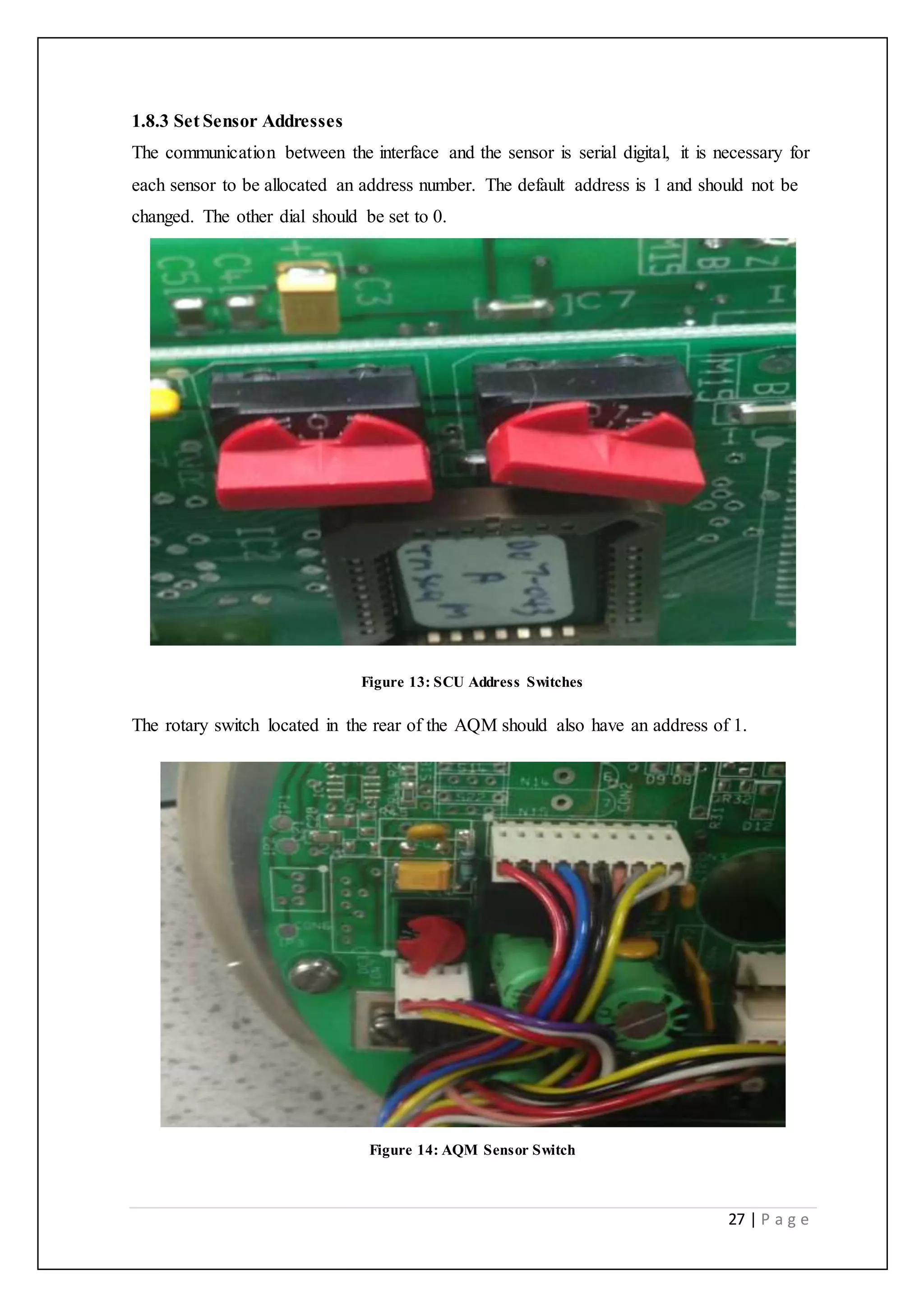
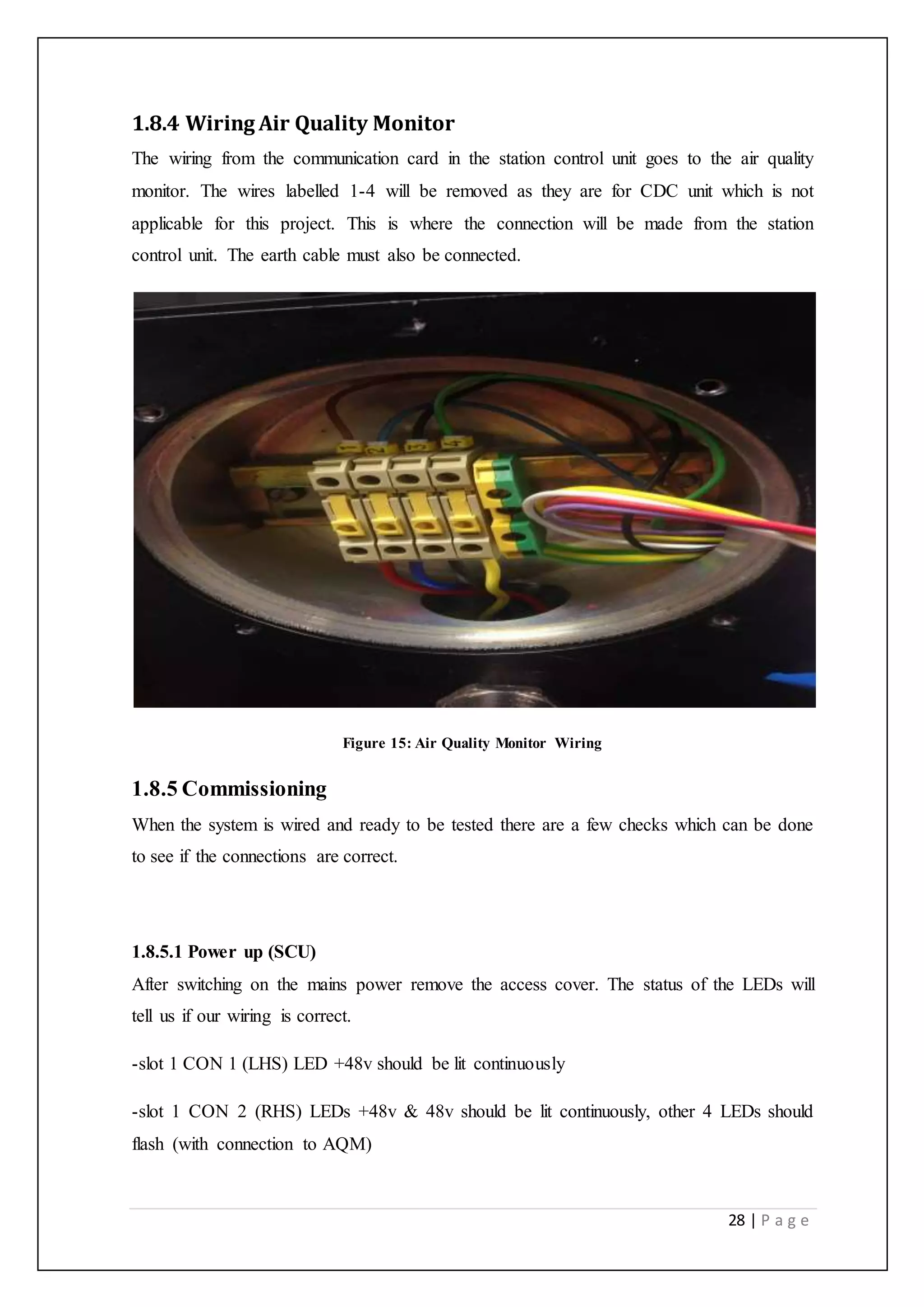
1.8 Device Wiring
1.8.1 Wiring Power Supply Unit
The wiring of the power supply unit is straight forward with the mains power coming in
top right hand side of the unit. The live, neutral and earth connections are wired in here.
Figure 10: Power Supply Unit [1]
The 48v outputs will be wired into the current outputs card in the station control unit.

26. 25 | P a g e
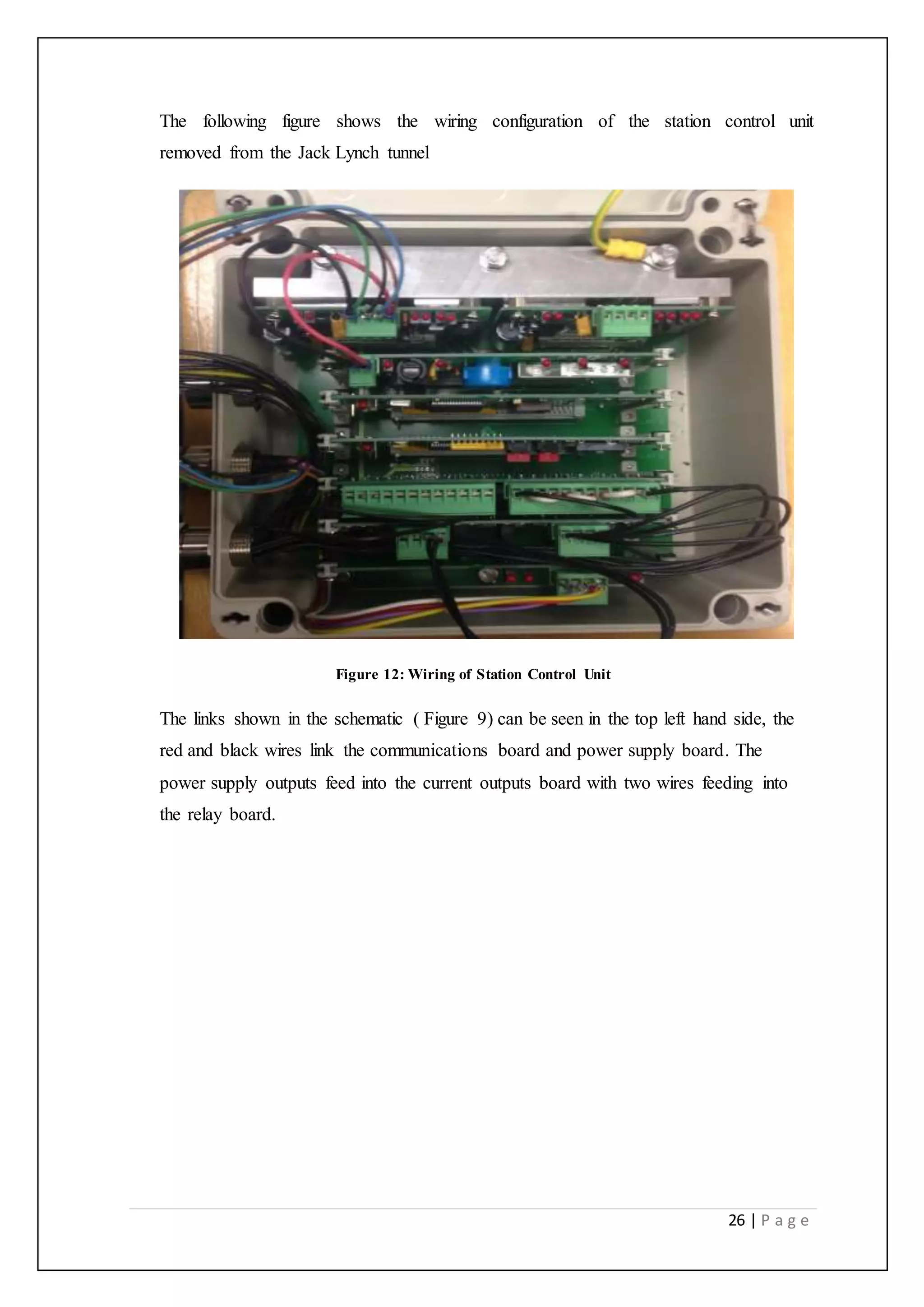
1.8.2 Wiring Station Control Unit
The wiring of the station control unit is more complex but the following schematic
provides excellent graphic illustration of what is required.
Figure 11: Station Control Unit Schematic [1]
 Keep links in place are important wire connections from the power supply unit to
the air quality monitor
 The output from the power supply unit is connected into the power supply card
seen in the above schematic
 The communications card is wired into the air quality monitor connectors (red,
blue, black, yellow) on the bottom left of the above schematic
 The power supply is wired into the power supply card in the SCU and to the current
output card and the relay card
 The RS232 communications is connected into the users laptop operating WinCom
software

27. 26 | P a g e
The following figure shows the wiring configuration of the station control unit
removed from the Jack Lynch tunnel
Figure 12: Wiring of Station Control Unit
The links shown in the schematic ( Figure 9) can be seen in the top left hand side, the
red and black wires link the communications board and power supply board. The
power supply outputs feed into the current outputs board with two wires feeding into
the relay board.

28. 27 | P a g e
1.8.3 Set Sensor Addresses
The communication between the interface and the sensor is serial digital, it is necessary for
each sensor to be allocated an address number. The default address is 1 and should not be
changed. The other dial should be set to 0.
Figure 13: SCU Address Switches
The rotary switch located in the rear of the AQM should also have an address of 1.
Figure 14: AQM Sensor Switch

29. 28 | P a g e
1.8.4 Wiring Air Quality Monitor
The wiring from the communication card in the station control unit goes to the air quality
monitor. The wires labelled 1-4 will be removed as they are for CDC unit which is not
applicable for this project. This is where the connection will be made from the station
control unit. The earth cable must also be connected.
Figure 15: Air Quality Monitor Wiring
1.8.5 Commissioning
When the system is wired and ready to be tested there are a few checks which can be done
to see if the connections are correct.
1.8.5.1 Power up (SCU)
After switching on the mains power remove the access cover. The status of the LEDs will
tell us if our wiring is correct.
-slot 1 CON 1 (LHS) LED +48v should be lit continuously
-slot 1 CON 2 (RHS) LEDs +48v & 48v should be lit continuously, other 4 LEDs should
flash (with connection to AQM)

30. 29 | P a g e
-slot 2 all LEDs on card should be lit continuously
-slot 3 HB LED should flash
-slot 4 HB LED should flash
-slot 7 LED 5 should be lit with LEDs Tx & Rx flashing when communicating through
RS232 port
1.9 Installation
1.9.1 Mounting AQM
The air quality monitor should be mounted horizontally on the wall.
1.9.2 Alignment of AQM Sensor
The alignment from the transceiver to the reflector is key for optimum performance. Both
pieces of equipment are fitted with universal adjustment features at the bottom of their
brackets. For correct alignment, observe the reflection in the mirror and both circles should
be concentric. Final alignment can be made using the application software.

31. 30 | P a g e
Chapter 2
Experimental Setup

32. 31 | P a g e
2.1 Wiring the Device
The device was wired as laid out in the introduction with no complications.
Figure 16: Device Wired
 The PSU is the top box and the SCU the bottom box
 The mains supply is wired into the top right of the PSU box
 The output from the PSU +48V & 0V is wired into the power supply card in the
SCU unit

33. 32 | P a g e
 The link wires between the PSU unit and the AQM are the two small red wires in
the bottom left hand side of the SCU box
 The four long red wires went to the AQM (see below)
Figure 17: AQM Wired
 The top right hand side of the SCU box is the RS232 communications port which
feeds into the system running Codel’s software

34. 33 | P a g e
2.1.1Wiring the RS232 Communications
The RS232 connection had to be soldered together, the following schematic was used:
Figure 18: RS232 Female Pin out [13]
The connection was soldered together using the above pin out.
Figure 19: RS232 Soldered Connection

35. 34 | P a g e
2.2 Software Configuration
2.2.1 Alignment
The device must be aligned before use, the sensor and reflector must be carefully aligned
for the full capabilities of the sensor. However, for the purpose of this project the sensor
was not mounted on a wall which it is designed for. The device was operated while being
situated on a window sill in the air quality lab above the college car park. This location was
chosen to monitor the pollutant concentrations from the car park traffic. For the device to
work to work to its full capabilities it should be perfectly aligned which would require
proper mounting and installation of the device.
To align the device the AQM should be fixed and the reflector should be tweaked as it is
more sensitive to movement of the two. For optimum performance the desired readings are
CO = 90 and VIS = 60. An error of ±5 is accepted for data recording.
Figure 20: Detector Aligned
Black background on the alignment screen indicates the data is okay, if the background is
red (figure 21) it indicates the device is saturated.

36. 35 | P a g e
Figure 21: Saturated Detector
The background can flash blue also; this means there is a communication error. It is
common for the occasional blue flash during transmission. When the sensors are
completely out of line we get a reading of 0 for Vis and 255 for CO & NO.
Figure 22: Detector Misalignment

37. 36 | P a g e
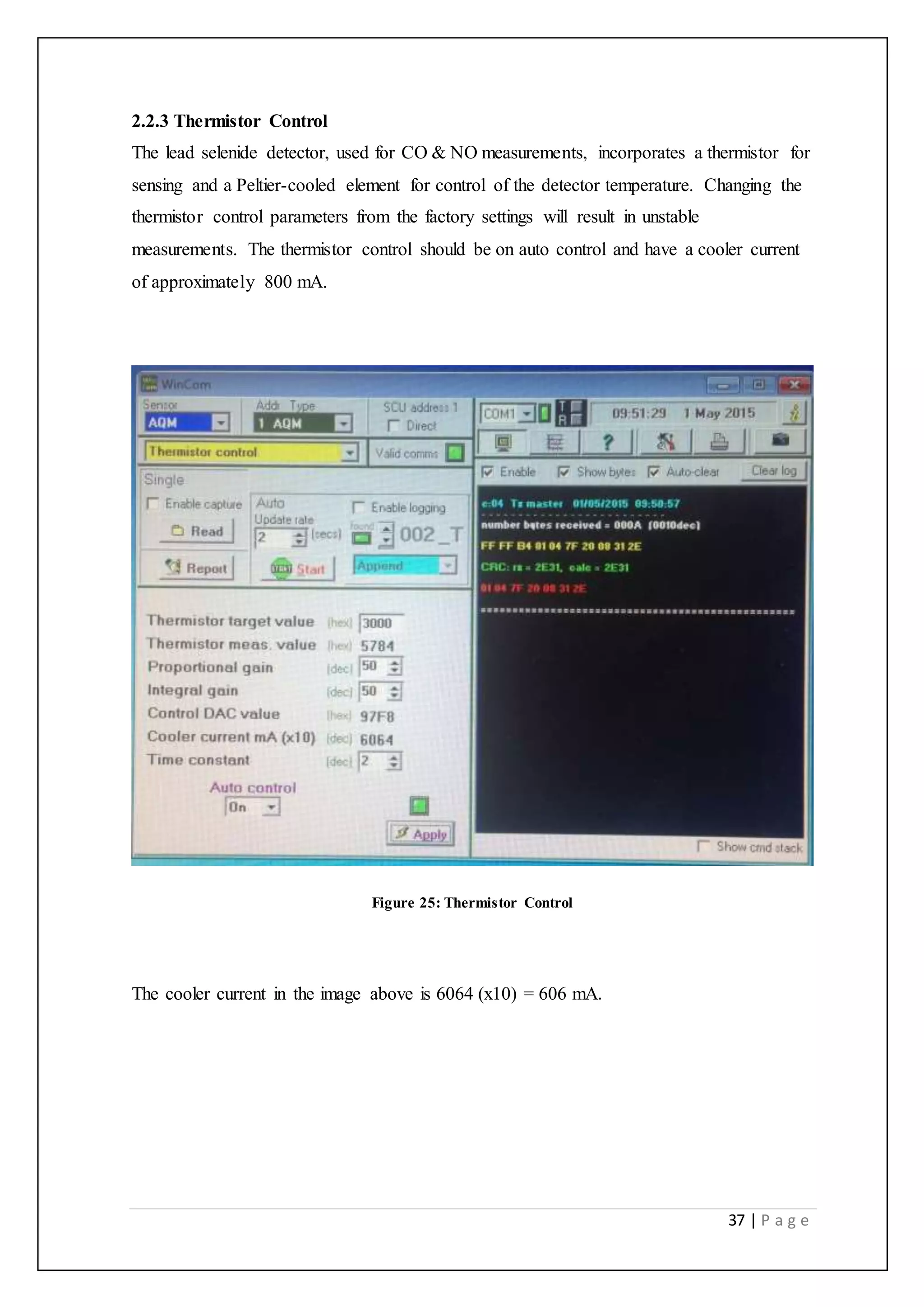
2.2.2 Detector Levels
The detector levels indicate the typical ranges for the measurements parameters. The
following image indicates the typical ranges for correct performance:
Figure 23: Detector Levels Range [1]
The measurement process will indicate a detector saturation condition by switching the
saturation indicator from green to red if the signal strength of the detector is too high. The
gain should be reduced if the red indicator is observed.
Figure 24: Detector Level Saturated
Vis Rx is saturated; this can happen if the path length is too short. (3m is recommended)

38. 37 | P a g e
2.2.3 Thermistor Control
The lead selenide detector, used for CO & NO measurements, incorporates a thermistor for
sensing and a Peltier-cooled element for control of the detector temperature. Changing the
thermistor control parameters from the factory settings will result in unstable
measurements. The thermistor control should be on auto control and have a cooler current
of approximately 800 mA.
Figure 25: Thermistor Control
The cooler current in the image above is 6064 (x10) = 606 mA.

39. 38 | P a g e
2.2.4 Output
The output mode displays output value data for CO, NO and visibility channels. The
standard output screen is below and this indicates the device is in calibration mode. (See
calibration 2.2.6)
Figure 26: Output Configuration
 The opacity reading describes the transparency level, where 1 is not transparent and
0 is fully transparent. Opacity will increase as CO & NO levels increase.
 Vis metres will decrease as our CO & NO levels increase, this is expected as the
more gas present in the path length the less visibility

40. 39 | P a g e
2.2.4.1 Instantaneous v Smoothed measurement
The software allows data to be measured in two forms, instantaneous and smoothed. An
instantaneous measurement is the data measured at that particular instant. Smoothed
measurements are the data measured averaged over a time period.
2.2.5 Y-Values
These values are used by the processor to compute concentration levels for CO & NO in
ppm. The standard output screen is below and this indicates the device is under zero gas
conditions.
Figure 27: Y-Values
The Y value can be calculated and checked using the calibration data.

41. 40 | P a g e
1. Y (CO) = 90,000 – (Set Cal CO) * CO Measured / CO Reference
90,000 – (55,118) * (13,608 / 9,397)
= 10,182 Actual value for Y (CO) = 10,241
2. Y (NO) = 90,000 – (Set Cal NO) * NO Measured / NO Reference
90,000 – (57,092) * (10,045 / 7,149)
= 9781 Actual value of Y (NO) = 9,818
2.2.6 Calibration
Like any measurement system Codel’s AQM must be calibrated regularly to maintain
highly accurate and reliable data. To calibrate select ‘ON’ and click ‘APPLY’. Please note,
after a power-up and after an interruption of the optical beam for more than 10 seconds, the
instrument automatically switches to calibration mode for 240 minutes and 30 minutes
respectively. The automatic calibrations can be stopped by selecting ‘Send’ screen and
sending the file ‘calstop.dtx’ to the AQM master processor.
Figure 28: Stop Calibration

42. 41 | P a g e
After the file is sent it takes approximately 10 seconds and a relay trip can be heard in the
station control unit box. Then select calibrate ‘OFF’ and the device will be forced out of
calibration mode.
2.3 Testing
2.3.1 Overnight data recording
The device was left recording data from 6pm-12am the next day; it recorded small levels
of CO ranging from 0-5 ppm. This is expected as the device location is 20 m from the
small car park.
The following images are CO and visibility levels at 11am.
Figure 29: CO Overnight Recording
There is a correlation between CO levels rising (0 to 5 ppm) and Visibility levels falling
(9999 to ~825).
Figure 30: Visibility Overnight Recording

43. 42 | P a g e
2.3.2 Bump Test
The idea of the bump test (also known as spike test) is to introduce high levels of gases
into the device and the data measurements should record the spike in readings. It proves
the system is recording data and also checks the range of the instrument. To do a bump test
the system had to be sealed to allow the sensor record the data rather than it escaping into
the atmosphere .The gas sample was acquired from the exhaust from a petrol engine car.
The system was crude and simple but sufficient for the purpose of this experiment. A
plastic pipe was used to connect the sensor to the reflector with the ends sealed with soft
tissue. The gas bag had an extraction pipe and a valve to control the flow and this was fed
into the inlet valve located on the centre of the pipe.
Figure 31: Experimental Set-Up

44. 43 | P a g e
 CO levels went from 0 – 1376 ppm before the device was over saturated and cut
into calibration mode
 No levels went from 0 – 10 ppm
 Opacity went from 0 – 60 and slowly decreased back down as gas escaped to 0
(fully transparent air)
 Vis metres went from 9999 – 1872 as the gas entered the system and the clear
transparent air got replaced with polluted fumes.
Note: Further analysis of the bump test is done in the results section 3.2.1 and 3.2.2
2.3.3 Cross Calibration Test
The next experiment undertaken was a cross calibration of Codel’s AQM and Alpha Sense
CO sensor. CO levels were compared between the two. The experimental setup for this
was similar to bump test with the addition of an outlet pipe leading the gas into the alpha
sense probe before it exited the system. The red lines show the gas flow.
Figure 32: Cross-Calibration Test
The alpha sense probe is on the left hand side of the above picture in a sealed plastic
container.
Note: Detailed analysis of the cross calibration test is done in the results section.

45. 44 | P a g e
2.3.4 Technical Specs for Carbon Monoxide Alpha Sense Probe
 Measuring units are ppm
 Measurement range of 0-1000 ppm, this is the range for which the error obtained
does not exceed the maximum permissible error
 Temperature range of -30°C to 50°C
 Sensitivity in 400 ppm CO is 55 to 90, this is ability to respond to small physical
differences
 Response time from 0 – 400 ppm CO is < 25, this is the time taken by the sensor to
approach its true output after being subject to corresponding input
 Zero Drift ppm equivalent change/year in a lab of < 0.2
 Resolution ppm equivalent < 0.5, this is the smallest change a sensor can detect in
the quantity that it is measuring

46. 45 | P a g e
Chapter 3
Analysis of Results

47. 46 | P a g e
3.1 Ambient Monitoring
The test involved the Codel sensor monitoring ambient air from 12 pm to 1 am the
following day, the maximum CO reading per half hour was plotted against the time of day.
Figure 33: Ambient Monitoring (CO)
The data monitoring proved inconclusive with the max CO reading recorded being 3 ppm.
With the accuracy of the sensor being +/- 1 ppm these small readings could be contributed
to noise. The location of the sensor was 20m from the car park and with no air being
pumped into the lab where the device is located on the window sill; the low readings
recorded are no surprise.
0
0.5
1
1.5
2
2.5
3
3.5
12:00:00 PM1:40:48 PM3:21:36 PM5:02:24 PM6:43:12 PM8:24:00 PM10:04:48 PM11:45:36 PM1:26:24 AM
CO(ppm)
Time of Day
Ambient Monitoring (CO)

48. 47 | P a g e
3.2 Bump Tests
3.2.1 Bump Test 1
The test was undertaken for Codel’s AQM with safety measures in place as carbon
monoxide is highly dangerous in high concentrations. Carbon monoxide was forced from
the gas bag into the sealed system via the inlet tube (See figure 31).
Figure 34: Bump Test 1 (CO)
The device read CO levels from 0 ppm up to 1376ppm before the device was over
saturated and the instrument cut into calibration. The sensor went into calibration outside
the specified operating range (1376 ppm > 1000 ppm) which is expected. Nitric Oxide
(NO) also spiked slowly from 0-10 ppm but the main pollutant present from exhaust
emissions was the carbon monoxide.
0
200
400
600
800
1000
1200
0 50 100 150 200 250
CO (ppm)
Time (s)
AQM Bump Test 1 (CO)

49. 48 | P a g e
Figure 35: Bump Test 1 (NO)
3.2.2 Bump Test 2
The test was repeated the following day after the system was flushed out and re-aligned
and calibrated.
Figure 36: Bump Test 2
The results were similar with the sensor reading CO levels from 0 ppm up to 1464 ppm
before the device was over saturated and cut into calibration mode.
0
2
4
6
8
10
12
0 50 100 150 200 250 300 350 400 450 500
NO(ppm)
Time (s)
AQM Bump Test 1 (NO)
0
200
400
600
800
1000
1200
0 50 100 150 200 250
CO (ppm)
Time (s)
AQM Bump Test 2 (CO)

50. 49 | P a g e
Codel’s software also graphs the data; the y axis needs a multiplier of X100. A section of
the graph can be magnified by clicking and dragging the cursor across the required area.
Figure 37: Codel's Graph Plot
Codel’s air quality monitor has a measurement range of 0 – 1000 ppm. Above 1000 ppm
the sensor becomes over saturated and the device cuts into calibration. (1464 ppm here)
While the gas enters the sealed system the air molecules become flushed with gas
molecules leaving the visibility in the system to decrease. This is an important parameter
when the device is installed in a busy tunnel. The following image is the visibility curve as
gas was forced from gas bag into the system. The Y axis has a multiplier of x100 with
units of metres.

51. 50 | P a g e
Figure 38: Visibility Graph
 Vis metres went from 9999 – 1872 as the gas entered the system and the clear
transparent air got replaced with polluted fumes.
The troughs are subject to the force being placed on the gas bag and the influx of gas
molecules decreasing the visibility of air, while the system is sealed for the gas to remain
in the pipe long enough for the sensor to read the gas levels, the gas will escape at the pipe
ends causing the crest effect.

52. 51 | P a g e
3.3 Cross CalibrationTest
The comparison test was done with alpha sense probe which range is also 0 -1000 ppm.
The gas was fed from the air quality monitor to the alpha probe with both instruments
recording CO levels.
Figure 39: Cross Calibration Test
We can see the correlation of data with both instruments recording similar CO levels. The
difference in the data is due to the system design; the data shows gas escapes from the
system before reaching the Alpha Sense probe. However, the correlation of the probes
shows the instruments recording accurate concentrations of carbon monoxide.
0
200
400
600
800
1000
1200
0 100 200 300 400 500
C0(ppm)
Time (s)
Codel & Wolfesense Comparison
Codel
Wolfesense

53. 52 | P a g e
3.4 Report Generation
The software also allows the user to generate a report at any time and records all readings
at that time (Y values, thermistor, detector levels, output, and calibration).
Figure 40: Report Generation
 The serial number of the air quality monitor used is stated 0298
 In this report the output of CO is 1317 ppm
 The high concentrations recorded cause the CO detector levels (range 15000-
25000) to crash down to ~4500

54. 53 | P a g e
Chapter 4
Concluding Remarks

55. 54 | P a g e
4.1 Discussion
The air quality monitor was wired from the schematics provided in the instrument manual.
The station control unit (SCU) was connected for communications and the power supply
unit (PSU) to the mains supply. A RS232 connection was used to transfer data from the
SCU to the PC running Codel’s software. The main issue for testing and calibration of the
instrument was the alignment. The device is designed for horizontal mounting on a wall.
The project was done with the device resting on window sill and alignment of the device
was extremely tough and time consuming, small movements as little as one millimetre can
cause miss-alignment. Post-test the device can be saturated and needs a settling time along
with re-calibration which can take up to four hours; this made the testing phase difficult.
CO & NO measurements were taken for installation purposes for Cork Institute of
Technology with possible sites being the mechanics workshop were combustion engines
are used indoors and the work yard were deliveries take place. Co levels up to 15 ppm
were recorded and with a resolution of 1 ppm for codel’s sensor this would be a viable
option for installation.
4.2 Future Work
Recommended installation and mounting of the device would improve the sensor’s
alignment and increase the accuracy of measurements recorded and allow the device to be
used to its full capabilities. Another recommendation is to install network infrastructure to
allow remote access to the device.
4.3 Conclusion
The air quality monitor was re-commissioned back to working order with all wiring done
as per schematics in the manual. Codel’s WinCom software was installed to run the device;
it is connected via the RS232 connection in the station control unit. The sensor and
reflector were carefully aligned with the path length being the recommended 3 m (6 m
folded beam).Pre alignment the senor had to be calibrated; the software includes an inbuilt
calibration function which takes up to 4 hours after a power up. The device was left
monitoring ambient air from the nearby car park but the test proved inconclusive as the
maximum CO value recorded was 3 ppm. With the accuracy of the sensor being +/- 1 ppm

56. 55 | P a g e
the small levels detected could be down to noise. With no air being pumped into the lab
were the device was located it was going to be a struggle to pick up plausible readings. The
working status of the device was checked via a bump test using gaseous fumes from a car
exhaust. The sensor’s range is 0-1000 ppm for CO and the bump test showed the device
being saturated and cutting out at 1376 ppm CO. Nitric oxide levels were not heavily
present as the NO output went from 0 – 10 ppm. The increase in pollution caused an
expected consequential decrease in visibility. Visibility dropped from full visibility reading
of 9999 to low visibility of 1872. This effected the opacity reading which went from 0
(fully transparent air) to 60 (semi-transparent air). The sensor operated under as expected
under the extreme influx of pollutants. The sensor was compared with another leading
manufacturer of CO probes called Alpha Sense, the system design was modified (See
figure 32) with the gas entering codel’s path length before travelling to the alpha probe, the
correlation of data showed similar CO values with alpha probe recording slightly less CO
concentrations which is expected due to some gas escaping in the system at each end of the
plastic pipe. This validated the integrity of the measurements by Codel’s air quality
monitor by comparing it with the measurements recorded by the standard lab device sensor
(Alpha Sense). The device was re-commissioned back to working order, calibrated by the
WinCom software and validated by the cross calibration test with the laboratory probe
(Alpha Sense). Overall the project was a success and the required tasks were
accomplished.

57. 56 | P a g e
References
1. http://en.wikipedia.org/wiki/Carbon_monoxide_poisoning
2. Codel Tunnel Craft 3 technical manual
3. http://www.detcon.com/electrochemical01.htm
4. FPO. (2004). Electrochemical gas detector and method of using same. Available:
http://www.freepatentsonline.com/4141800.html. Last accessed 20 Feb 2015.
5. Muda, R. (2009). Simulation and measurement of carbon dioxide exhaust
emissions using an optical-fibre-based mid-infrared point sensor. Journal of Optics
A: Pure and Applied Optics, 11(1)
6. Figaro Sensor. (2003). General Information for TGS Sensors. Retrieved February
28, 2010, from http://www.figarosensor.com/products/general.pdf
7. Naranjo, E. (2007). Ultrasonic Gas Leak Detectors. Retrieved February 27, 2010,
from http://www.gmigasandflame.com/article_october2007.html
8. Codel. (2011). Tunnel Atmosphere Monitoring. Available:
http://www.forbesmarshall.com/fm_micro/downloads/Codel/AQM.pdf. Last
accessed 20 Feb 2015.
9. Sense Air. (2000). Measuring method for emissions in road tunnel
systems. Available: http://senseair.se/wp-content/uploads/2011/05/14.pdf. Last
accessed 24th Feb 2015.
10. Csep. (2015). Atomic absorption and emission spectra. Available:
http://csep10.phys.utk.edu/astr162/lect/light/absorption.html. Last accessed 3rd
May 2015.
11. SenseAir. (2010). Gas Application. Available:
http://www.senseair.se/senseair/gases-applications/carbon-monoxide/. Last
accessed 3rd May 2015.
12. 11.Electro-Optics. (2010). Silicon Photo detectors. Available:
http://www.eotech.com/cart/category4/photodetectors/silicon-photodetectors. Last
accessed 20 Feb 2015.
13. 12.Servomex. (2009). Gas filter correlation. Available:
http://ww3.servomex.com/gas- analyzers/technologies/gas-filter-correlation. Last
accessed 20 Feb 2015.
14. http://pixshark.com/rs232-female-pinout.htm