FAULT ANALYSIS AND CIRCUIT BREAKERS SELECTION FOR ELECTRICAL LINES PROTECTION: CASE OF ELECTRICAL LINE FROM LUTCHURUKURU TO KINDU (D.R. CONGO)

International Journal of Computer Science, Engineering and Applications (IJCSEA)
Vol. 15, No.3/4/5, October 2025
DOI : 10.5121/ijcsea.2025.15502 21
FAULT ANALYSIS AND CIRCUIT BREAKERS
SELECTION FOR ELECTRICAL LINES
PROTECTION: CASE OF ELECTRICAL LINE FROM
LUTCHURUKURU TO KINDU (D.R. CONGO)
M N Audry 1
, H Shabani 1,2
, J Fisher 2
and J Ngondo 1,3
1
Electrical Engineering, MAPON University, Kindu-Maniema, Democratic Republic
of Congo (D.R. Congo)
2
School of Electrical and Communications Engineering, Papua New Guinea
University of Technology (Unitech), Lae 411, Morobe Province, Papua New Guinea
3
North China Electric Power University, 02, Beinong Lu, Changping, Beijing, China
ABSTRACT
Consumption of electrical energy has steadily increased due to industrial, commercial and
demographic growth. In order to deliver constant power to consumers, reliability is an important
factor that power companies must take into account. Common disturbances on transmission lines
resulting from various faults such as line to line, single line to earth, double line to earth and faults
between three lines affect the stability of the electric supply. This paper seeks to demonstrate the
behavior of transmission line signals due to disturbances caused by different types of faults and to
identify the effect of faults on transmission lines as well as on the bus assembly. Simscape Power tool
available in MATLAB/Simulink environment was used to model the 33 kV, 105 km transmission line. Its
simulation made it possible to obtain the voltage and the current wave forms in the transmission
network during the occurrence of different fault types. The electrical faults cause down time equipment
damage and, thus, present a high risk to the integrity of the power grid. After various fault analysis of
the power line from Lutchurukuru to Kindu, the circuit breakers to be placed at the transmitting and
receiving ends of this power line were selected with the aim of reinforcing the power line protection
system. Hence, the circuit breakers at the transmitting end (Bus 2) of the line must have a breaking
capacity of 4.376 MA, a voltage of 34.5 kV, a number of cycles for the fault interruption time of 5 and a
sub transient fault current of 49.15 A, while the ones placed at the receiving end (Bus 7) of the line
must have a breaking capacity of 497.5 kA, a voltage of 34.5 kV, 5 number of cycles for fault
interruption and a sub transient fault current of 5.6 A.
KEYWORDS
Transmission lines, reliability, faults, Circuit breaker, MATLAB/Simulink
1. INTRODUCTION
For the transmission and distribution of electrical energy, the lines are the vital links to ensure
the continuity of services to users, the latter are exposed to atmospheric and natural conditions
which increase the probability of appearance of any type of faults [1]. Faults in power lines
occur in unusual conditions due to climate (Lightning, strong Wind, tremors, weight of ice on
conductors, trees, contaminated or broken insulators, corona not controlled, aircraft and cars
hitting lines and structures) [2] and human errors. The analysis of faults forms an important
step on the study of electrical system; the problem consists of determining the bus voltages

Vol. 15, No. 3/4/5, October 2025
22
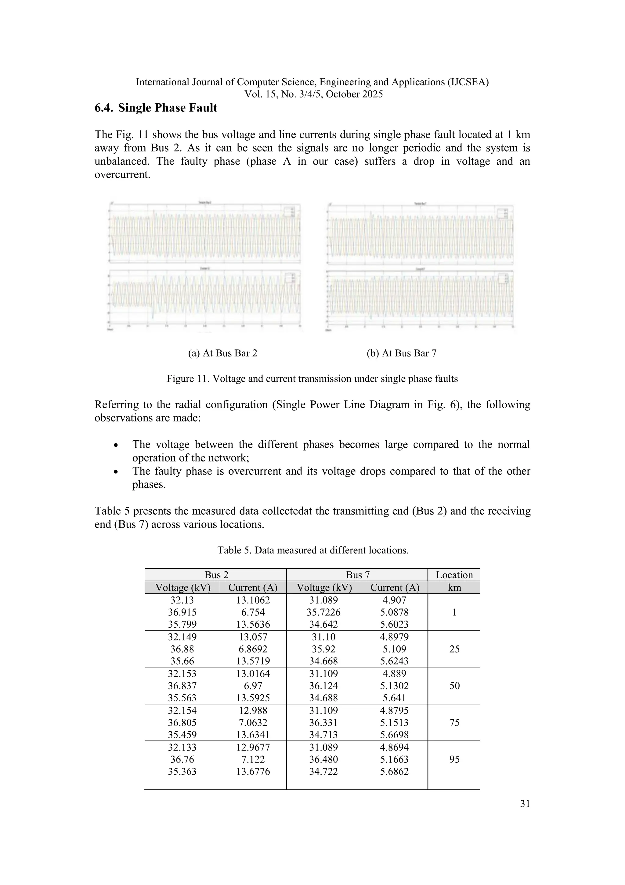
and the line current during the appearance of different types of faults. Faults on electrical
equipment are subdivided into two categories including balanced three phase faults and
unbalanced faults (single phase fault, two phase fault, fault between two phases and earth) [3].
The information obtained after fault analysis is necessary for the parametrization and
coordination to obtain the nominal values of the protective equipment [4].
However, the electrical line from Lutchurukuru to Kindu requires reinforcement in its
protection system, along this line it is found certain protective devices such as fuse holder
disconnectors (already defective and replaced by bare wires in the open air), Lightning
arrestors, but there are no circuit breakers at both ends of this line or a relay for faults
detection and isolation of defective areas. Maniema is supplied with electricity by the
Lutchurukuru power station via a 105 km power line [5]. This paper analysesvarious faults
that may appear in this line during operation which will make it possible to make a good
choice of protection devices and to configure the monitoring device to thus, protect this line
and to guarantee residents of the town of Kindu with continuous and reliable power supply.
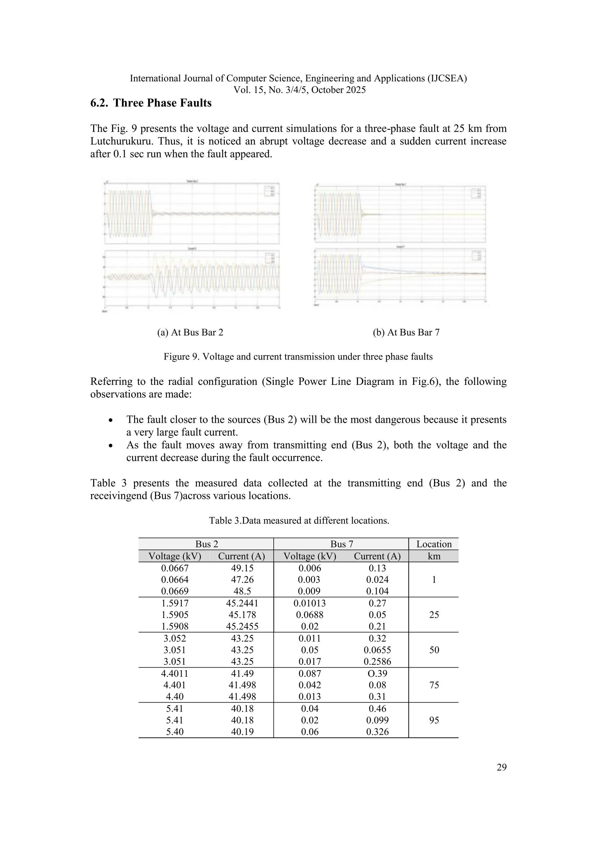
The main goal is to present the behaviour of bus voltage and line currents during normal and
faulty operating conditions. The following steps were undertaken before circuit breaker
selection to ensure the protection of the Lutchurukuru Kindu line by:
 Modelling of Lutchurukuru-Kindu Power Network;
 Simulating the network, under normal conditions;
 Simulating various types of faults in the power line;
 Selecting appropriate circuit breakers for the power line protection.
The above simulations were carried out on the Simulink environment.
2. FAULTS IN POWER SYSTEMS
In general, the balanced systems only exist in theory, in reality many systems are almost
unbalanced and for practical reasons they can be analysed as balanced. However, there are
emergency conditions (open conductors, unbalanced loads…) where the degree of unbalance
can no longer be neglected. To protect the system against such eventualities, it is necessary to
size protection devices such as fuses, circuit breakers and to adjust protection relays [6]. To
do this the voltage and currents in the system during unbalanced faults must be known in
advance. Faults in electrical lines can be classified into two type, series faults (open
conductors) and shunt faults (short circuit). Series faults are easily identified by observing the
value of each phase voltage [7]. If the fault voltage value is zero it indicates that fault has
occurred, in case current value increases it means a shunt fault has occurred. Short circuit
faults may be asymmetrical (line to ground, line-to-line, double line to ground) or
symmetrical (triple line and triple line to ground) [1], [8]. On Fig. 1 we observe the
classification of faults in overhead transmission lines where A, B, C and G indicate
respectively the three phases and the ground.

Vol. 15, No. 3/4/5, October 2025
23
Figure 1. Faults classification [7].
2.1. Fault Effects
Heavy short circuit may cause damage to equipment or any other element of the power
system due to overheating or flashover, different phenomenon may be observed [9], [10];
 There may be reduction in the supply voltage of the healthy feeders, resulting in the
loss of industrial loads.
 Short circuit may cause the unbalance of the supply voltages and currents, thereby
heating rotating machines.
 There may be a loss of the power stability
 The faults may cause an interruption of the supply to consumers;
Thoughtful result of the uncleared faults, is fire which may not destroy only the equipment of
its origin but also may spread within the system and cause total failure.
2.2. Faults types in Transmission Lines
Normally a power system operates under balanced conditions. When the system is unbalanced
due to the insulation failures at any point or due to the contact of live wires, a short circuit or
fault is said to occur [1]. Faults that occur in transmission lines are classified into two groups
as:
 Symmetrical faults
 Asymmetrical faults.
1. Symmetrical faults.It is a fault which appears when all three phase conductors are short
circuited, the latter gives balanced faults currents. Three phase to ground fault is
shown in the following Fig. 2.

Vol. 15, No. 3/4/5, October 2025
24
Figure 2. Symmetrical faults.
For this type of fault, it should be noted that:
 Symmetrical faults rarely appear in practice since the majority of faults are non-
symmetrical.
 The symmetrical fault is the most dangerous since it imposes a large fault current on
the circuit breakers.
1. Asymmetrical faults.These faults lead to unequal currents with unequal phase shifts in a
three-phase system. This may occur by natural disturbances or by human errors with
open conductors or short circuit [11]. As presented in the Fig. 3, asymmetrical faults
are generally classified as:
 Single line to ground fault (L – G fault)
 Double line fault (L – L fault)
 Double line to ground fault (L – L – G fault)
Figure 3. Asymmetrical faults.
The single line to ground (L – G fault) is the most current fault (60 to 75% of occurrence).
They appear when a conductor of transmission line falls to earth or during contact between
the latter and the neutral conductor [1]. A fault between two phases appears in an electrical
line when two conductors are short circuited (L – L fault). The occurrence frequency rate of
this fault type fluctuates between 5 to 15%. The fault between two phases and earth in
transmission line appears when two conductors fall and are connected together across the
neutral (L – L – G fault). The occurrence frequency rate of this fault type fluctuates between
15 to 25% [12]. A fault study comprises the following [3]:
 Determination of the maximum and minimum three phase short-circuit currents;
 Determination of asymmetrical fault currents;
 Rating evaluation of required circuit breakers;
 Investigation of schemes of protective relaying;
 Determination of voltage levels at strategic points during faults.

Vol. 15, No. 3/4/5, October 2025
25
3. TRANSMISSION LINE PROTECTIVE DEVICES
Transmission system must be protected from short circuit currents, which can endanger personnel and
cause permanent damages to critical equipment [13]. To guarantee a safely isolation of the system
faulty parts, the fault current must not exceed the capacity of the circuit capacity device [14]. Various
types of protection devices in transmission systems as shown in Fig. 4.
Figure 4. Various protective devices.
The purpose of protective device is to detect abnormal signals in the power transmission
system [2]. A protection system consists of a set of devices intended for fault and abnormal
situation detection in networks in order to control the triggering of cutting elements. The
functional chain of a protection system includes one part for fault detection and another part
for fault elimination [12], [15]. As presented in Fig. 5, whatsoever the technology, the
protection system is made up of the following three fundamental parts [16]:
 Sensors or measuring reducers which lower the values to be monitored (current,
voltage) to levels usable by the protection;
 Protective relays;
 Switching equipment (one or more circuit breakers).
Figure 5. Fundamental elements of protective systems.
At the receiving end of the line there is a similar protection system, in the event of a fault the
circuit breaker opens and the line is taken out of service [16].
3.1. Fault Location
Different techniques and methods have been introduced on fault location estimation; among
them impedance-based faults location methods are the most used by utilities [17]. Based on
the input data (voltage and current) of fault location algorithm, the algorithms can be
categorized as:

Vol. 15, No. 3/4/5, October 2025
26
 One end algorithm method which is economic and simple but subjected to different
errors such as the uncertainty of transmission lines, unbalanced load flow, the
accuracy of transmission line model [18], and measurement errors. With this method
the location of fault is based on the impedance from one end of a transmission line
[19].
 Two end algorithm method which estimates the location of fault using voltage and
current from both ends of a transmission line [20].
3.2. Circuit Breaker Selection
When a fault appears the protection devices are activated (relay and circuit breaker). A short
time called tripping time elapsing before the protection relay detects the overcurrent and
launches the tripping pulse to the circuit breaker [21]. For the circuit breaker to open, another
time called opening time passes. The circuit breaker opening is accompanied with an arc
which is extinguished after a duration called arc time. The time from which the tripping pulse
is launched until the arc is extinguishing is called interruption time. The speed of the circuit
breaker will therefore be recognized according to the time which elapses between the
appearance of the fault and extinction of the arc [22]. The selection of circuit breakers is
based on the following factors [1]:
 Class of the voltage considered (nominal effective voltage level);
 The load current that the circuit breaker must withstand in the normal or emergency
condition;
 The short circuit current that the circuit breaker must withstand;
 The speed of interruption of the short circuit (the latter depends on the number of
interruption cycles and the network frequency.
The load current in normal operation can be found by studying the power flow of the circuit
to be protected [23]. The short circuit data determines the selection of the circuit breaker by
taking into account the operating voltage [24]. In general, the quicker the circuit breaker
interrupts a fault, the better it is for the system because there is a reduction in the risk of
damage devices [25], [26].
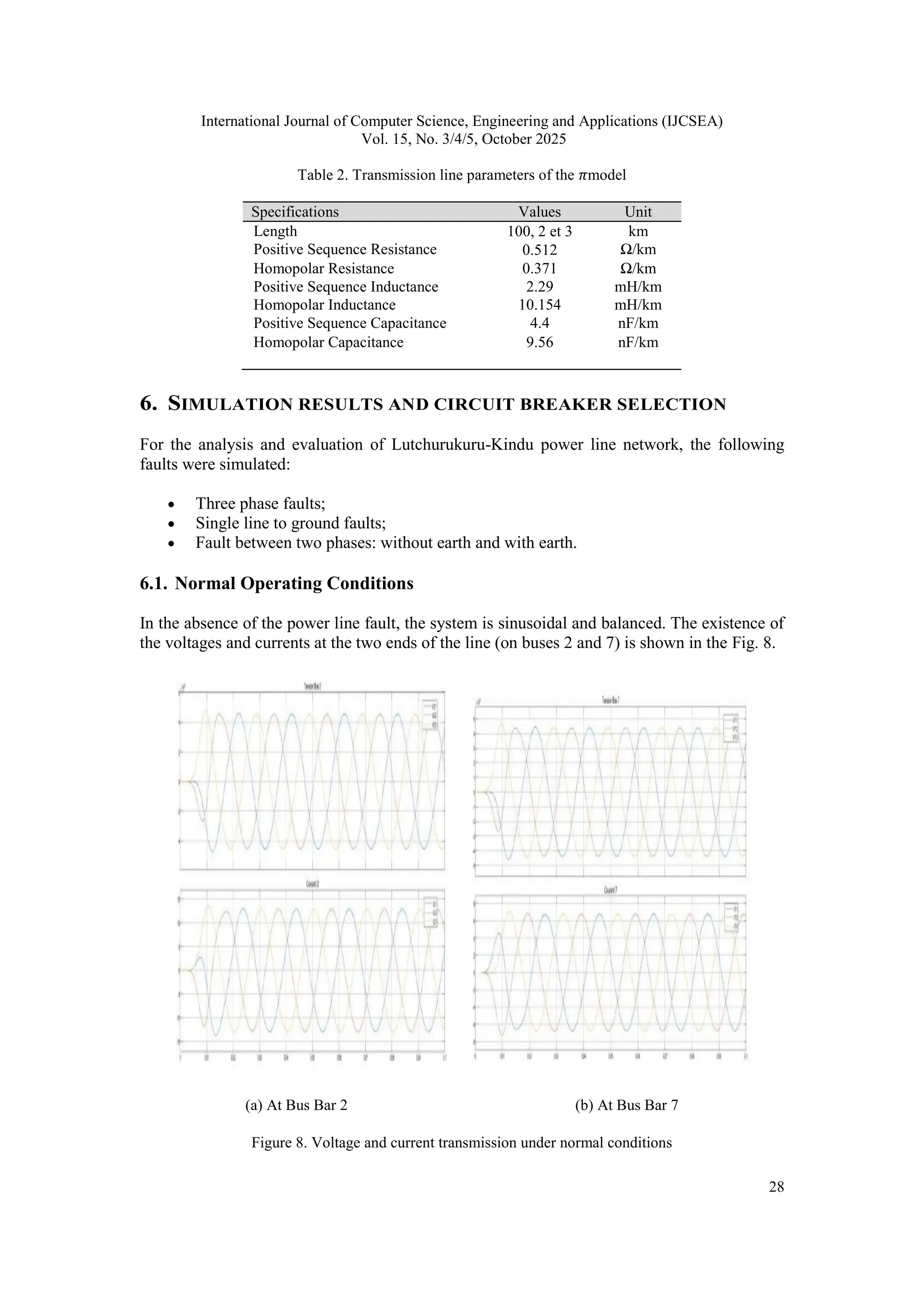
4. DESCRIPTION OF LUTCHURUKURU – KINDU NETWORK
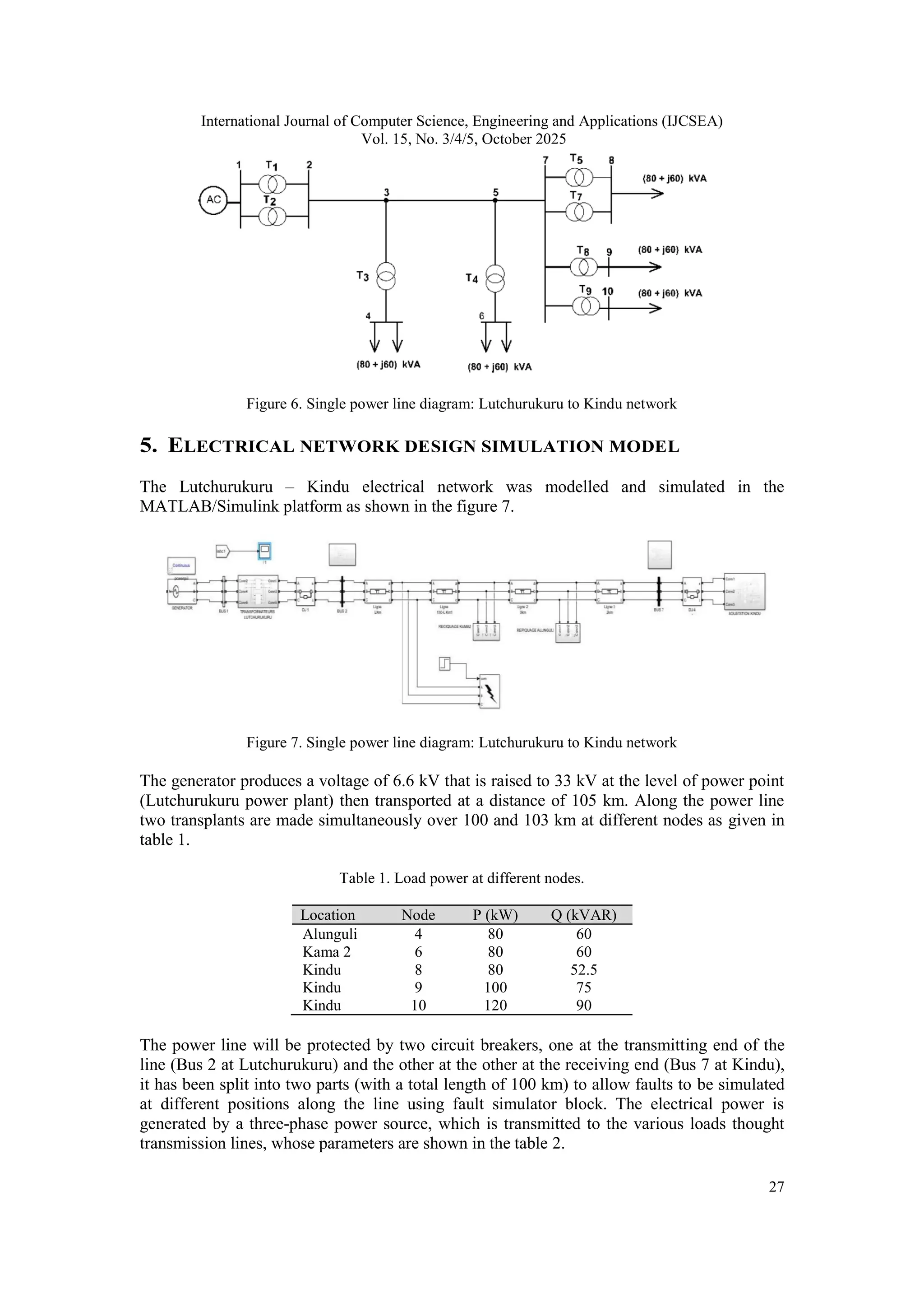
TheFig. 6 illustrates the single power line diagram of Lutchurukuru to Kindu network. The
Lutchurukuru power plant is designed with 3 turbo alternator groups of 2700 kVA each, but
currently only one remains working with a power production of around 500 kW. The output
voltage is 6.6 kV. The transformer station is located at the outlet of the power plant where two
2 MVA transformers are placed in parallel which raise the voltage up to 33 kV for its
transport to the town of Kindu located approximately at 105 km where the overhead line stays
on pillars of 10 m in height. It is a three-phase line with one terminal, its phase conductors
have a diameter of 50 mm.

Vol. 15, No. 3/4/5, October 2025
27
Figure 6. Single power line diagram: Lutchurukuru to Kindu network
5. ELECTRICAL NETWORK DESIGN SIMULATION MODEL
The Lutchurukuru – Kindu electrical network was modelled and simulated in the
MATLAB/Simulink platform as shown in the figure 7.
Figure 7. Single power line diagram: Lutchurukuru to Kindu network
The generator produces a voltage of 6.6 kV that is raised to 33 kV at the level of power point
(Lutchurukuru power plant) then transported at a distance of 105 km. Along the power line
two transplants are made simultaneously over 100 and 103 km at different nodes as given in
table 1.
Table 1. Load power at different nodes.
Location Node P (kW) Q (kVAR)
Alunguli 4 80 60
Kama 2 6 80 60
Kindu 8 80 52.5
Kindu 9 100 75
Kindu 10 120 90
The power line will be protected by two circuit breakers, one at the transmitting end of the
line (Bus 2 at Lutchurukuru) and the other at the other at the receiving end (Bus 7 at Kindu),
it has been split into two parts (with a total length of 100 km) to allow faults to be simulated
at different positions along the line using fault simulator block. The electrical power is
generated by a three-phase power source, which is transmitted to the various loads thought
transmission lines, whose parameters are shown in the table 2.

Vol. 15, No. 3/4/5, October 2025
28
Table 2. Transmission line parameters of the 𝜋model
Specifications Values Unit
Length 100, 2 et 3 km
Positive Sequence Resistance 0.512 Ω/km
Homopolar Resistance 0.371 Ω/km
Positive Sequence Inductance 2.29 mH/km
Homopolar Inductance 10.154 mH/km
Positive Sequence Capacitance 4.4 nF/km
Homopolar Capacitance 9.56 nF/km
6. SIMULATION RESULTS AND CIRCUIT BREAKER SELECTION
For the analysis and evaluation of Lutchurukuru-Kindu power line network, the following
faults were simulated:
 Three phase faults;
 Single line to ground faults;
 Fault between two phases: without earth and with earth.
6.1. Normal Operating Conditions
In the absence of the power line fault, the system is sinusoidal and balanced. The existence of
the voltages and currents at the two ends of the line (on buses 2 and 7) is shown in the Fig. 8.
(a) At Bus Bar 2 (b) At Bus Bar 7
Figure 8. Voltage and current transmission under normal conditions

Vol. 15, No. 3/4/5, October 2025
29
6.2. Three Phase Faults
The Fig. 9 presents the voltage and current simulations for a three-phase fault at 25 km from
Lutchurukuru. Thus, it is noticed an abrupt voltage decrease and a sudden current increase
after 0.1 sec run when the fault appeared.
Figure 9. Voltage and current transmission under three phase faults
Referring to the radial configuration (Single Power Line Diagram in Fig.6), the following
observations are made:
 The fault closer to the sources (Bus 2) will be the most dangerous because it presents
a very large fault current.
 As the fault moves away from transmitting end (Bus 2), both the voltage and the
current decrease during the fault occurrence.
Table 3 presents the measured data collected at the transmitting end (Bus 2) and the
receivingend (Bus 7)across various locations.
Table 3.Data measured at different locations.
Bus 2 Bus 7 Location
Voltage (kV) Current (A) Voltage (kV) Current (A) km
0.0667 49.15 0.006 0.13
1
0.0664 47.26 0.003 0.024
0.0669 48.5 0.009 0.104
1.5917 45.2441 0.01013 0.27
25
1.5905 45.178 0.0688 0.05
1.5908 45.2455 0.02 0.21
3.052 43.25 0.011 0.32
50
3.051 43.25 0.05 0.0655
3.051 43.25 0.017 0.2586
4.4011 41.49 0.087 O.39
75
4.401 41.498 0.042 0.08
4.40 41.498 0.013 0.31
5.41 40.18 0.04 0.46
95
5.41 40.18 0.02 0.099
5.40 40.19 0.06 0.326

Vol. 15, No. 3/4/5, October 2025
30
6.3. Two Phase Faults
The Fig. 10 shows the bus voltage and line currents during two phase faults located at 1 km
away from Bus 2. As it can be seen the signals are no longer periodic and the system is
unbalanced. The effective values vary according to the fault location.
Figure 10. Voltage and current transmission under two phase faults
 Two phases remain powered unlike the three-phase fault;
 The absence of voltage in the third phase.
Table 4 presents the measured data collectedat the transmitting end (Bus 2) and the
receiving end (Bus 7) across various locations.
Table 4. Data measured at different locations.
27.838 9.1558 26.926 4.7757
1
0.066 45.5244 0.0033 2.3867
27.821 36.6604 26.926 2.3897
28.203 9.1587 26.925 4.7758
25
3.0517 41.9228 0.003 2.3867
27.535 33.1006 26.925 2.3909
28.029 9.1578 26.925 4.7754
50
3.0159 43.5960 0.003 2.3865
27.534 34.7281 26.924 2.23901
28.345 9.1529 26.912 4.7752
75
4.4026 40.3606 0.002 2.3865
27.4556 31.5933 26.912 2.23904
28.461 9.1517 26.916 4.77
95
5.410 39.2081 0.001 2.3878
27.434 30.48 26.916 2.3916

Vol. 15, No. 3/4/5, October 2025
31
6.4. Single Phase Fault
The Fig. 11 shows the bus voltage and line currents during single phase fault located at 1 km
away from Bus 2. As it can be seen the signals are no longer periodic and the system is
unbalanced. The faulty phase (phase A in our case) suffers a drop in voltage and an
overcurrent.
Figure 11. Voltage and current transmission under single phase faults
Referring to the radial configuration (Single Power Line Diagram in Fig. 6), the following
 The voltage between the different phases becomes large compared to the normal
operation of the network;
 The faulty phase is overcurrent and its voltage drops compared to that of the other
phases.
Table 5 presents the measured data collectedat the transmitting end (Bus 2) and the receiving
end (Bus 7) across various locations.
32.13 13.1062 31.089 4.907
1
36.915 6.754 35.7226 5.0878
35.799 13.5636 34.642 5.6023
32.149 13.057 31.10 4.8979
25
36.88 6.8692 35.92 5.109
35.66 13.5719 34.668 5.6243
32.153 13.0164 31.109 4.889
50
36.837 6.97 36.124 5.1302
35.563 13.5925 34.688 5.641
32.154 12.988 31.109 4.8795
75
36.805 7.0632 36.331 5.1513
35.459 13.6341 34.713 5.6698
32.133 12.9677 31.089 4.8694
95
36.76 7.122 36.480 5.1663
35.363 13.6776 34.722 5.6862

Vol. 15, No. 3/4/5, October 2025
32
6.5. Double Phase to Ground Faults
A fault between two phases and ground is different from a two phases fault because the faulty
conductors touch the earth. The Fig.12 shows the bus voltage and line currents during double
phase to ground fault located at 1 km away from Bus 2. As it can be seen the signals are no
longer periodic and the system is unbalanced. The faulty phase (phase A in our case) suffers a
drop in voltage and an overcurrent. The fault closer to Bus 2 leads to an overcurrent and drop
in voltage atBus 2. When the fault moves away from Bus 2, the current drops and the voltage
rises.
Figure 12. Voltage and current transmission under double phase to ground faults
 Two phases remain powered with unwanted voltages;
 The third phase presents a low voltage and an overcurrent.
Table 6 presents the measured data collectedat the transmitting end (Bus 2) and the receiving
end (Bus 7) across various locations.
28.973 9.4827 28.030 4.9756
1
0.066 45.7980 0.003 2.4862
28.956 36.4016 28.03 2.4901
28.795 9.5075 27.707 4.9
25
1.5911 43.86 0.0032 2.4535
28.425 34.488 27.707 2.4572
29.215 9.6953 28.011 4.9675
50
3.0531 42.3325 0.003 2.4822
28.573 32.6808 28.011 2.4865
29.473 9.7715 28.186 4.9977
75
4.4017 40.8369 0.00218 2.4974
28.627 31.1164 28.186 2.5020
29.683 9.7218 28.322 5.0344
95
5.4104 39.6531 0.0011471 2.5160
28.665 29.9890 28.322 2.5208

Vol. 15, No. 3/4/5, October 2025
33
6.6. Circuit Breaker Selection
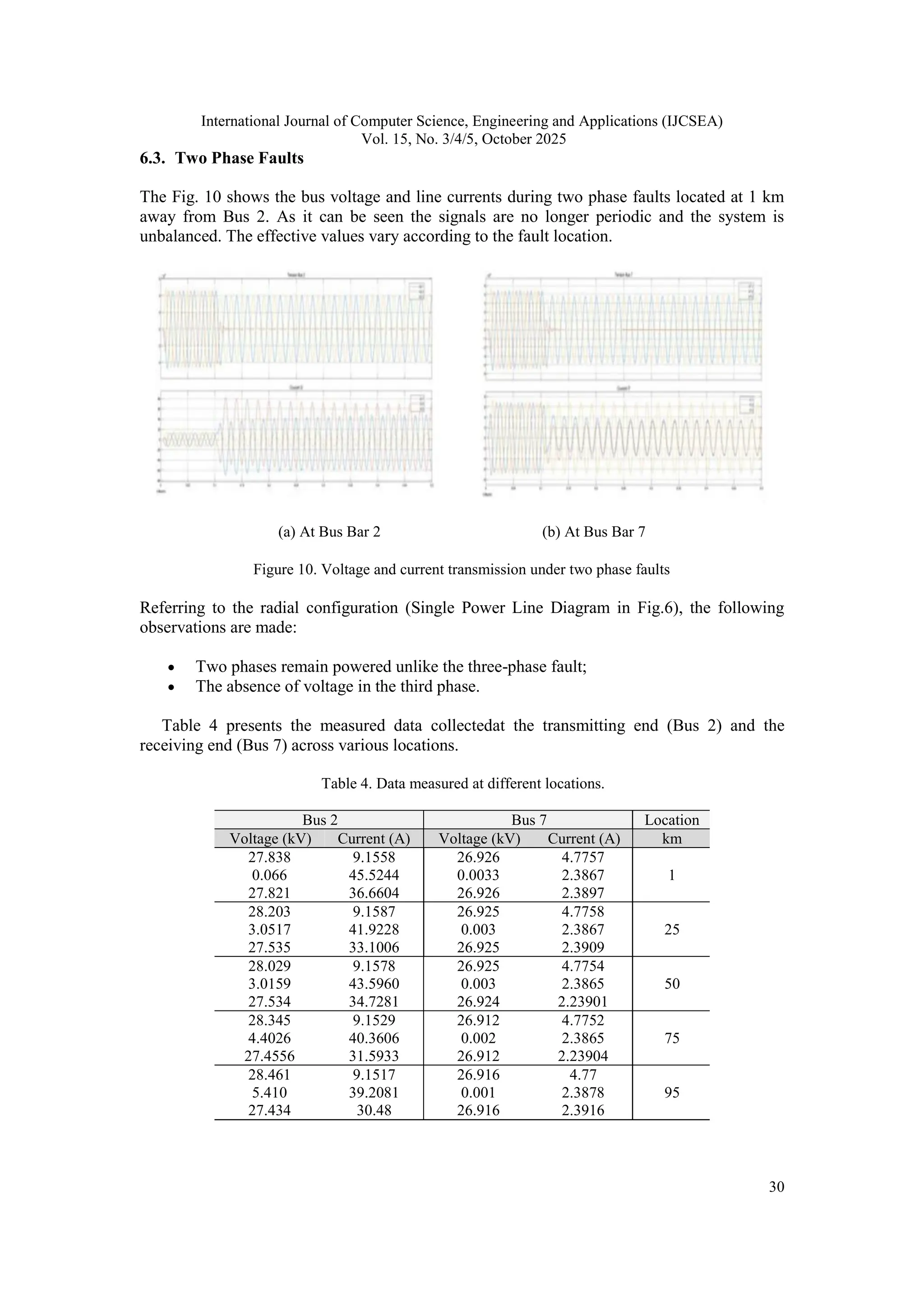
After analysing all the faults along the line, it was found that the three-phase fault is the most
dangerous because it has the greatest fault current measured at Bus 2. Using data from normal
working voltages and fault currents the circuit breakers to be placed respectively at the
transmittingend and receiving end of the line are presented in the following table 7 and table 8
respectively.
Table 7. Circuit breaker characteristics
at the transmitting end (Bus 2)
Normalized Voltage 34.5 kV
Steady State Current 9.4 A
Sub transient Fault
Current
49.15 A
Number of Cycles for
Interruption Time
5
Breaking Capacity 4.376 MA
Maximum
Instantaneous Current
139.017 A
Maximum Value of
DC Component
69.5 A
Momentary Current 78 A
𝑆𝑚𝑜𝑚𝑒𝑛𝑡𝑎𝑛é 4.376 MVA
Table 8. Circuit breaker characteristics
at the receiving end (Bus 7)
Normalized Voltage 34.5 kV
Steady State Current 4.77 A
Sub transient Fault
Current
5.6 A
Number of Cycles for
Interruption Time
5
Breaking Capacity 497.5 kA
Maximum
Instantaneous Current
15.84 A
Maximum Value of
DC Component
8 A
Momentary Current 8.96 A
𝑆𝑚𝑜𝑚𝑒𝑛𝑡𝑎𝑛é 482.41 VA
𝑆 𝑚𝑜𝑚𝑒𝑛𝑡𝑎𝑛é: time-varying value of apparent power
7. CONCLUSION
The presented results in this paper deal with the analysis of numerous types of faults and
selection of circuit breakers for the protection of power lines. To determine the behaviour of
the network during transient conditions, the power line network model and its simulation
were carried out using Simscape power tool box available in Simulink. Hence, referred to the
measured data in table 3, the three phase fault at figure 9, has been identified as the most
dangerous fault because it generates a greater fault current at the transmitting end (Bus 2).
Hence, the data collected during the three-phase fault analysis were used to decide on the
characteristics of the circuit breakers to deploy in both transmitting and receiving ends of the
105 km long radial overhead power line power from Lutchurukuru to Kindu.
ACKNOWLEDGMENTS
Authors would like to thank the School of Electrical and Communications Engineering at the
Papua New Guinea University of Technology (Unitech) for funding the publication of this
paper.
REFERENCES
[1] T. Gonen, “Alectric Power Transmission System Engineering Analysis and Design,” New York:
CRC Press.
[2] S. H. a. F. Ayalew, “Fault Detection, Protection and Location on Transmission Line,”
Researchgate, p. 9, 21 decembre 2021.
[3] S. A. Nasar, “Theory and Problems of Electric Power Systems,” McGRAW-HILL.
[4] V. M. e. R. Mehta, “Principles of Power System,” S. CHAND.

Vol. 15, No. 3/4/5, October 2025
34
[5] D. Snel, “Interviewee, Protective equipement for the Lutchurukuru Kindu power Line.”
[Interview]. 24 January 2024.
[6] B. Mohamed, “Coordination des Systemes de Protection,” Algérie : Universite Constantine 1,
2013.
[7] O. S. e. al, “Signal Behaviours of Power Transmission Line During Fault,” IRE Journals, 2019.
[8] T. B. Satish Karekar, “A Modelling of 440 kV EHV Transmission line faults identified and
analysis by using MATLAB Simulation,” International Journal of Advanced Research in
Electrical, Electronics and Instrumentation Engineering , p. 8, 3 March 2016.
[9] H. Saadat, “Power System Analysis,” McGraw-Hill.
[10] R. Kumar, “Three Phase Transmission Lines Fault Detection, Classification and Location” ISJR,
p. 4, 2013.
[11] E. D. O. A. A. Abdullahi Afwah, “Three-Phase Fault Analysis on Transmission line In MATLAB
SIMULINK,” IJESRT, p. 4, 2019.
[12] M. D. P. a. M. P. J. Mr. Sandesh Gaikwad, “Basic Matlab Simulation of Faults within Power
System” International Journal of Engineering Sciences and Research Technology , p. 7, May
2020.
[13] A. N. A. S. S. Akshit Sharma, “Fault Analysis on three phase Transmission lines and its
detection,” International Journal of Advance Research and Innovation , p. 5, 15 June 2017.
[14] Y. O. P. A. O. O.-S. O. Naenwi, “Analysis of Three- Phase Transmission Line FaultUsing
Matlab/Simulink,” International Journal of advances in Engineering and Management ( IJAEM),
p. 8, 13 07 2021.
[15] T. M. Rimsha Fazaln Habib Ullah Manzoor, “Analysis of Relay Protection System Compârison
for Better Identification InHigh Voltage AC Transmission Lines,” Research Square, p. 16, 22
November 2021.
[16] B.Lazhar, “Protection des réseaux électriques,” Algérie : Université Echahid Hamma
Lakhdard'EL Oued, 2017.
[17] S. R. M. S. h. a. s. Mehfuz, “Experimental studies on impedance based fault location for long
transmission line,” SpringerOpen, p. 9, 2017.
[18] T. S. Kawady, “A practical fault location approach for double circuit transmission lines using
using single end data.,” IEEE Transactions on power delivery , pp. 18, 1166-1173, 2003.
[19] J. a. S. M. Izikowski, “Locating faults in parallel transmission line under availibilityoat of
complete measurement at one end,” IEEE proceedings - Generation Transmission and distribution
, pp. 151, 268-273, 2004.
[20] R. M. Izykowski, “Fault location on double circuit series-compensated lines using two end
unsynchronised method measurement,” IEEE transactions on power delivery. , pp. 2072-2080,
2011.
[21] V. M.P. Thrake, “Distance Protection for Long Transmission Line using Pscad,” International
Journal of Advances in Engineering ang Technologie, pp. 2579-2586, January 2014.
[22] C. Prévé, “Protection of Elecrical Network,” 2006.
[23] N. e. al, “Analysis of Three Phase Transmisssion Line Fault using Matlab/Simulink,” IJAEM, p.
8, 2021.
[24] M. Y. N. K. S. Boora, “Matlab Simulation Based Study of Various Types of Faults Occuring in
the transmission Lines,” IJERT , p. 4, 12 December 2019.
[25] S. C. e. al, “Transmission Line Faultanalysis by using Matlab Simulation,” IJESRST, p. 4, 2015.
[26] J. D. Glover, “Power System Analysis and Design,” CENGAGE Learning.
[27] S. A. Nasar, “Theory and Problems of Electric Power Systems,” McGRAW- HILL, New York,
1990.

FAULT ANALYSIS AND CIRCUIT BREAKERS SELECTION FOR ELECTRICAL LINES PROTECTION: CASE OF ELECTRICAL LINE FROM LUTCHURUKURU TO KINDU (D.R. CONGO)

More Related Content

Similar to FAULT ANALYSIS AND CIRCUIT BREAKERS SELECTION FOR ELECTRICAL LINES PROTECTION: CASE OF ELECTRICAL LINE FROM LUTCHURUKURU TO KINDU (D.R. CONGO)

Recently uploaded

FAULT ANALYSIS AND CIRCUIT BREAKERS SELECTION FOR ELECTRICAL LINES PROTECTION: CASE OF ELECTRICAL LINE FROM LUTCHURUKURU TO KINDU (D.R. CONGO)