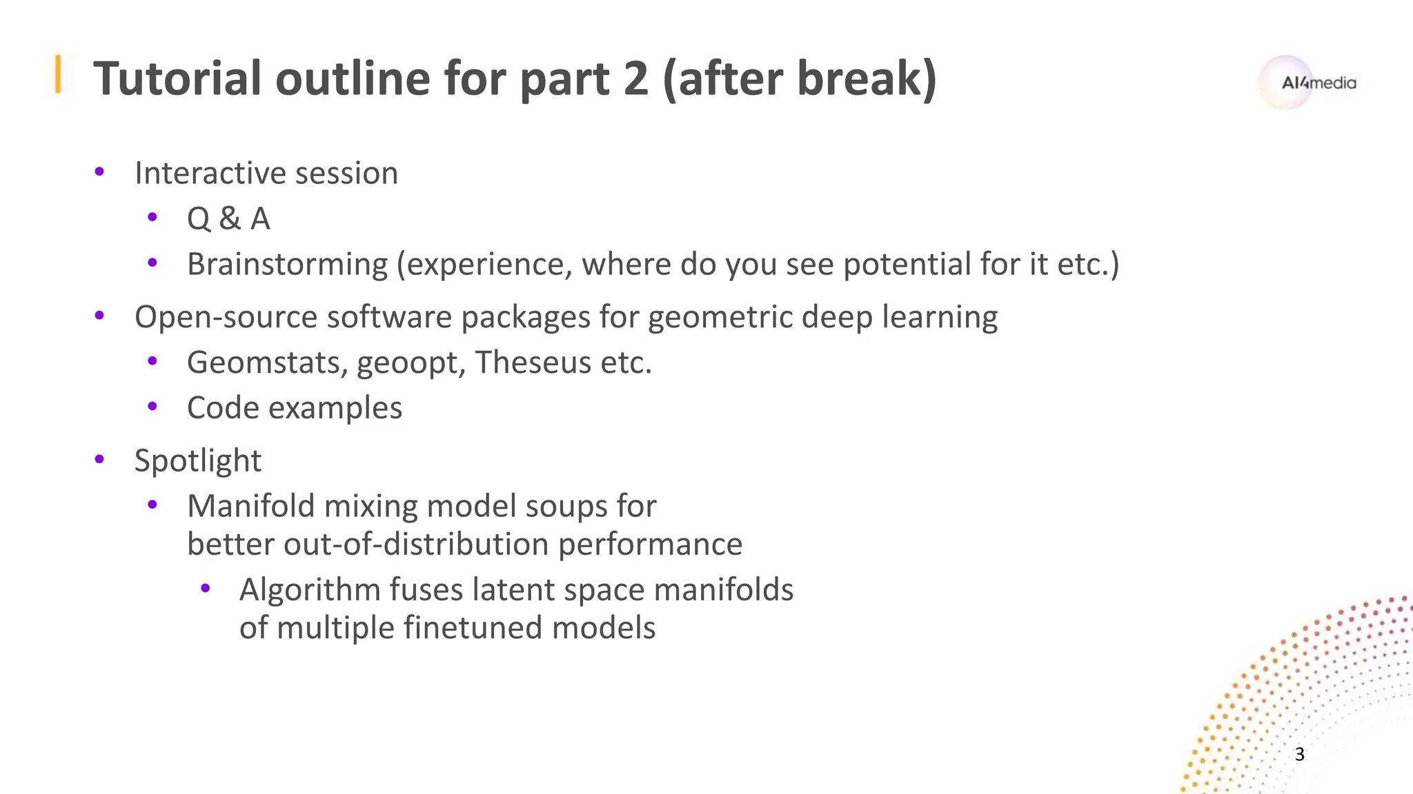
The document outlines a tutorial on geometric deep learning, focusing on its applications in multimedia, including image classification, synthesis, and video analysis. It covers fundamental concepts such as manifold theory, operations on manifolds, and presents various algorithms and open-source software packages for implementing these techniques. The tutorial also explores advanced uses of geometric deep learning, such as improving out-of-distribution performance and addressing challenges in non-Euclidean spaces.

1. 1
Geometric deep learning and
its application for multimedia
Hannes Fassold, JOANNEUM RESEARCH
MMAsia 2023 Tutorial
December 6-8, 2023
Tainan, Taiwan

2. Tutorial outline for part 1 (before break)
• Introduction into geometric deep learning (with a focus on manifolds)
• Motivation
• Key operations on manifolds
• Lie groups & Lie algebra
• Common manifolds used in computer vision
• Geometric deep learning algorithms in various multimedia applications
• Similarity search
• Image classification
• Image synthesis & enhancement
• Video analysis
• 3D data processing
• Nonlinear dimension reduction
2

3. Tutorial outline for part 2 (after break)
• Interactive session
• Q & A
• Brainstorming (experience, where do you see potential for it etc.)
• Open-source software packages for geometric deep learning
• Geomstats, geoopt, Theseus etc.
• Code examples
• Spotlight
• Manifold mixing model soups for
better out-of-distribution performance
• Algorithm fuses latent space manifolds
of multiple finetuned models
3

4. Introduction into
geometric deep learning
4

5. Introduction & motivation
• Classic neural networks are restricted to data lying in vector spaces
• But data residing in smooth non-Euclidean spaces
arise naturally in many problem domains …
• Examples for non-Euclidean spaces
• A 360 degree camera captures a “spherical” image
• Typically processed in equirectangular projection
• 2D/3D point meshes are an undirected graph
• E.g. as triangulation of a point cloud
• Rigid body transformations
• Employed in 3D photogrammetry, kinematics etc.
• Symmetric positive semidefinite matrices
• E.g. covariance matrices in diffusion tensor imaging (DTI)
5

6. Benefits of keeping algorithm in non-Euclidean space
• No need to find an auxiliary mapping to Euclidean space
• Like equirectangular projection for images from 360° camera
• Auxiliary mapping complicates algorithm workflow and
can lead to additional mathematical & numerical issues
• E.g. employing equirectangular projection leads to
problems like distortion, border ambiguity etc.
• Many research works are successfully employing non-Euclidean spaces
• E.g. DeepMind “GraphCast” algorithm
for weather forecast
• Utilizes a graph neural network
• Makes 10-day weather forecast
in less than one minute …
6

7. What is geometric deep learning ?
• Deep learning with data lying in non-Euclidean spaces
• Input layer – e.g. input data is a graph or covariance matrix
• Intermediate layer – e.g. we add a layer for a rigid body transformation
• Output layer – e.g. output is a “spherical” image
• Geometric deep learning usually deals with graphs or manifolds
• Graphs consist of vertices and edges
• Manifolds are well suited for generalizing a vector space
• Manifold M looks locally like
an d-dimensional Euclidean space
• E.g., a sphere is a 2-dimensional manifold
• Especially Riemannian manifolds are very useful
• This introduction will focus on (Riemannian) manifolds
7

8. A short primer into graph neural networks
• Many relations can be modeled as graphs
• Molecules, genes, social networks, knowledge graphs, …
• Important operators in graph neural networks (GNNs)
• Graph convolution
• Usually done employing
all neighbors of the node
• Graph laplacian
• Has same role in graphs as the
Laplace operator in Rd
• Resources
• See the survey by Wu et al [2]
• See also the blog article [3]
8
Normal convolution on 2D grid
versus graph convolution

9. Manifold & tangent space
• Manifold M of dimension d
• Is a topological structure which locally
(in the neighborhood of a point p ∈ M )
looks like a d-dimensional Euclidean space
• Tangent space TpM at point p ∈ M
• Best local approximation of “neighborhood” of p
with a d-dimensional Euclidian space
• Can be seen as linear approximation of M around p
• E.g. for a 2-dimensional manifold (like a sphere)
the tangent space TpM corresponds to
the tangent plane at point p
9

10. Curves and distances on a manifold
• Riemannian manifold
• Is a smooth manifold M equipped with an inner product gp
on the tangent space TpM of each point p
• Inner product g induces a norm on the tangent space
• Allows us to calculate curve lengths and distances on M
• Length of a curve c(t) on M can be calculated
by integrating the norm along the curve
• Geodesic for two points p and q
• Is a length-minimizing curve c(t) connecting p and q
• Geodesic distance d(p,q)
• Is the length of the geodesic c(t)
• Example: great-circle distance on the sphere
10
Great-circle distance d(P,Q)
on the sphere

11. Manifold operators – exponential map
• Exponential map
• p … (reference) point on M and
v … vector of its tangent space TpM
• Vector v is mapped now to the point q ∈ M
which is reached after unit time (t = 1)
by the geodesic c(t) starting at p
and going into the direction of v
• This mapping expp(v): TpM  M
is called the exponential map at point p
• Exponential map maps the tangent space TpM
to the manifold M
11

12. Manifold operators – logarithm map
• Logarithm map
• Mapping logp(q): M  TpM
is called the logarithm map at point p
• Inverse mapping to exponential map
• Is locally defined around a neighborhood of p
• Maps manifold to the tangent space
• Informal interpretation of exp/log
• Exponential map and logarithm map
move points back and forth between
the manifold and the tangent space(s)
in a distance-preserving way
12

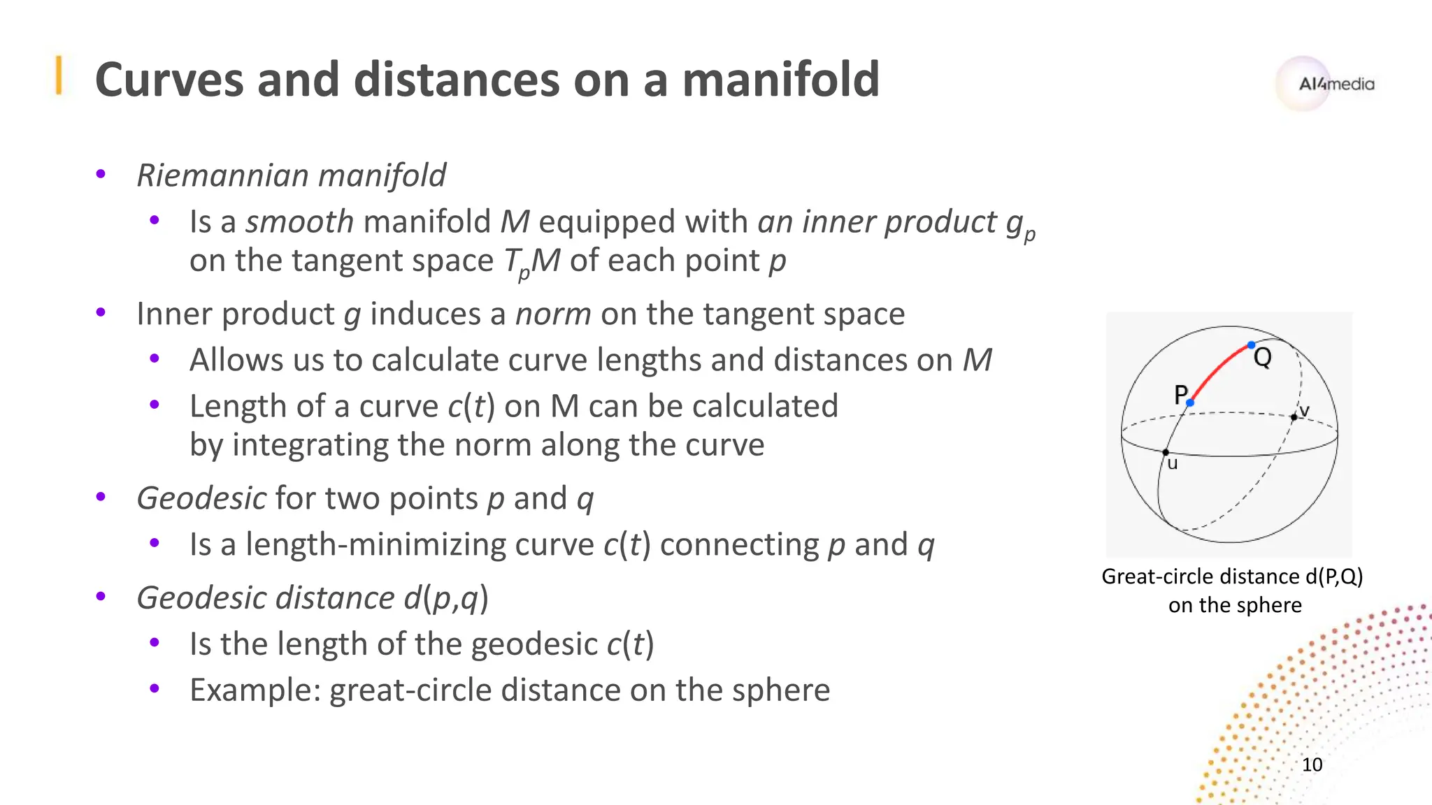
13. Manifold operators – Frechet mean
• Frechet mean (intrinsic mean)
• The Frechet mean of the points x1, ..., xn is the point  ∈ M which minimizes
the sum of the squared distances to all these points
• Formula:
• d(p,q) is the geodesic distance
• A weighted Frechet mean can be also defined
• In an Euclidean space, Frechet mean is identical
to the Euclidean mean (arithmetic mean)
• Usually calculated (approximately)
via an iterative algorithm
13
Frechet mean of three points
on a hyperboloid.
Image courtesy of [S-36]

14. Manifold operators – convolution
• Convolution operator can be defined in several ways on a manifold
• Via a weighted Frechet mean (see [SU-14], [SU-15], [SU-36])
• Via a weighted sum in the tangent space (see [SU-10])
• Convolution via a weighted sum in the tangent space – procedure
14

15. Manifold operators – other
• There is a variety of other useful operators on manifolds
• Parallel transport of a tangent vector along a curve
• Retraction is a first-order approximation (see [4])
of the exponential map which is faster to calculate
• Pullback operator
• Differential operators can be also defined on manifolds
• Intrinsic gradient
• Covariant derivative
• Divergence
• Laplacian
15
Parallel transport

16. Lie group and Lie algebra
• Lie group
• Is a smooth manifold that forms also a group
• Both group operations (usually called multiplication
& inverse) are smooth mappings of manifolds
• Lie algebra
• A Lie algebra of a Lie group M is defined
as the tangent space TeM at the identity e
• e … identity element of the group
• Lie groups provide also an exponential map
• May differ from the exponential map defined for Riemannian manifolds
• Is identical to matrix exponential for matrix Lie groups
• All compact Lie groups are matrix groups (follows from Peter-Weyl theorem)
16
Group axioms

17. Common manifolds used in computer vision
• Commonly employed (Riemannian) manifolds
• Sn … n-dimensional sphere
• SO(n) … n-dimensional rotation matrices (special orthogonal group)
• SE(n) … rigid body transformations (special euclidean group)
• Gr(n,p) … p-dimensional subspaces of Rn (Grassmann manifold)
• St(n,p) … p-dimensional orthogonal subspaces of Rn (Stiefel manifold)
• Pn … symmetric positive semidefinite matrices
17
Positive
semidefinite cone

18. Applications of
geometric deep learning
in multimedia
18

19. Similarity search & retrieval
• Identifying “hard” training examples
• Iscen et al, CVPR, 2018, ref. [SU-30]
• Useful e.g. for re-training with these
examples (curriculum learning etc.)
• Hard examples are identified
by comparing the distances
(similarities) measured via
• Euclidean distance
• Geodesic distance on the manifold
• Geodesic distance is calculated via
a random walk on the Euclidean
nearest neighbor graph
19

20. Similarity search & retrieval
• Robust metric learning with Grassmann manifolds
• Luo et al, AAAI, 2019, ref. [5]
• Traditional methods employ
L2 distance in feature space
• Sensitive to noise, as the
data distribution is usually
not Gaussian
• Method learns a projection from a
high-dimensional to a low-dimensional
Grassmann manifold
• Embedding distance (Harandi et al, [6])
is employed as distance on the
low-dimensional Grassmann manifold
20

21. Image classification & object detection
• Manifold mixup
• Verma et al, ICML, 2019, ref. [SU-50]
• Novel regularizer which forces the training to
interpolate between hidden representations
(captured in the intermediate network layers)
• Can be seen as a generalization of input mixup,
which does the interpolation on a random layer
• Input mixup uses always layer 0
• Positive effects of manifold mixup
• Flattens the class-specific representation
(lower variance)
• Generates a smoother decision boundary,
compare (a) and (b) in the right figure
21

22. Image classification & object detection
• Transfer CNN to 360° images
• Su et al, 2022, see [SU-50]
• Transfer an existing CNN model
trained on perspective images
to spherical images (from 360° camera)
without any additional annotation/training
• Faster R-CNN => Spherical Faster R-CNN
22

23. Image synthesis & enhancement
• Progressive Attentional Manifold Alignment for Arbitrary Style Transfer
• Luo et al, ACCV, 2022, ref. [SU-37]
• Progressively aligns content manifolds to their most related style manifolds
• Relaxed earthmover distance is used for alignment cost function
• Afterwards, space-aware interpolation is done in order to increase the
structural similarity of the corresponding manifolds
• Makes it easier for the attention module to match between them
23

24. Image synthesis & enhancement
• Image editing by manipulation of the latent space manifolds
• Parihar et al, ACM MM, 2022, ref. [SU-42]
• Performs highly realistic image manipulation with minimal supervision
• Estimates linear directions in the latent space of StyleGAN2 using a few images
• Introduces a novel method for sampling from the style manifold
24

25. Video analysis
• Geometry-aware algorithm for skeleton-based human action recognition
• Friji et al, CoRR, 2020, ref. [SU-27]
• Skeleton sequences are modeled as trajectories on
Kendall shape space and fed into a CNN-LSTM network
• Kendall shape space [7] is a quotient manifold which is invariant against
location, scaling and rotation (as these do not change the shape)
25

26. Video analysis
• DreamNet: Deep riemannian manifold network for SPD matrix learning
• Wang et al, ACCV, 2022, Ref. [SU-57]
• Adopts a neural network over the manifold Pn of
symmetric positive definite matrices as the backbone
• Appends a cascade of Riemannian autoencoders to it
in order to enrich the information flow within the network
• Experiments on diverse tasks (emotion recognition, hand action recognition
and human action recognition) demonstrate a favourable performance
26

27. 3D data processing
• Unsupervised Geometric Disentanglement for Surfaces via CFAN-VAE
• Tatro et al, ICLR, 2021, Ref. [SU-41]
• Novel algorithm for geometric disentanglement
(separating intrinsic and extrinsic geometry) of 3D models
• Surface features are described via a combination
of conformal factors and surface normal vectors
• Conformal factor defines a conformal
(angle-preserving) deformation
• Propose a convolutional mesh autoencoder
based on these features
• Algorithm achieves state-of-the-art performance
on 3D surface generation, reconstruction & interpolation
27

28. 3D data processing
• Intrinsic Neural Fields: Learning Functions on Manifolds
• Koestler et al, ECCV, 2022, Ref. [SU-33]
• Introduces intrinsic neural fields, a novel and versatile representation
for neural fields on manifolds
• Based on the eigenfunctions of the Laplace-Beltrami operator
• Intrinsic neural fields can reconstruct high-fidelity textures from images
28

29. Nonlinear dimension reduction
• DIPOLE algorithm
• Wagner et al, 2021, Ref. [SU-56]
• Corrects an initial embedding (e.g. calculated via Isomap) by minimizing
a loss functional with both a local, metric term and a global, topological term
based on persistent homology
• Unlike more ad hoc methods for measuring the
shape of data at multiple scales,
persistent homology is rooted in
algebraic topology and enjoys
strong theoretical foundations
29

30. Nonlinear dimension reduction
• SpaceMAP algorithm
• Tao et al, ICML, 2022, Ref. [SU-61]
• Introduces equivalent extended distance
• Makes it possible to match the
capacity between two spaces
of different dimensionality
• Performs hierarchical manifold
approximation, as real-world data
often has a hierarchical structure
30

31. - Questions ?
- Have you used geometric deep
learning already ?
- Where do you see its potential ?
31

32. Open-source
software packages for
geometric deep learning
32

33. Open source software packages - overview
• Packages had to fulfill the following criteria
• Open-source, in Python, with liberal license (Apache, BSD etc.)
• Riemannian manifolds
• Pymanopt
• Geoopt
• Geomstats
• Theseus
• Graph neural networks
• Pytorch Geometric (PyG)
• Nonlinear dimension reduction
• Paradime
33
Stable Diffusion Prompt: An image
showing a torus and a undirected graph

34. Pymanopt
• Supports all commonly used manifolds
• Sphere, symmetric positive definite matrices, Stiefel manifold,
Grassmann manifold, special orthogonal group, …
• Implements the standard operators on manifolds
• Norm, distance, exp, log, retraction, parallel transport etc.
• Provides a collection of optimizers
• For solving optimization problems directly on the manifold
• Gradient of the cost function is automatically calculated
(via automatic differentation functionality of Pymanopt)
• Steepest descent, conjugate gradients, Nelder-Mead,
rarticle swarm, Riemannian trust region
34

35. Pymanopt – code example
• Parameter estimation for Mixture of Gaussian models
• With Riemannian
manifold optimization
instead of
EM algorithm
• Employs a
product manifold of
SPD matrices
• Gradient of cost
function is calculated
automatically
35
Code snippet, full code available at https://github.com/pymanopt/pymanopt/blob/master/
examples/notebooks/mixture_of_gaussians.ipynb

36. Geoopt
• Compatible with Pytorch (uses Pytorch tensors, autodiff etc.)
• Supports also some more “exotic” manifolds
• Birkhoff polytope (double stochastic matrices), Poincare ball,
Hyperboloid (Minkowski) model,
• Sphere, symmetric positive definite matrices, Stiefel manifold,
Grassmann manifold, special orthogonal group, …
• Provides manifold-aware stochastic optimization algorithms
• SGD with Nesterov momentum, Adam
• Same interface as PyTorch optimizers
• Provides sampling from a probability distribution on the manifold
• Hamiltonian Monte-Carlo, Stochastic Gradient Langevin Dynamics,
Stochastic Gradient Hamiltonian Monte-Carlo
36

37. Geoopt – code example
• Birkhoff polytope
(manifold of
double stochastic
matrices)
• “closure” method
returns the loss
(like in Pytorch)
• Optimization with
Adam optimizer
37

38. Geomstats
• Supports roughly the same set of manifolds as geoopt
• Additionally also Kendall shape space [7] and statistical manifolds
• Statistical manifold is a Riemannian manifold where
each point is a probability distribution
(Binomial, Exponential, Normal, Poisson etc.)
• Implements some advance operators on manifolds
• Levi-Civita connection, Christoffel symbol, Ricci curvature
• Provides also some operators for statistical analysis
• Frechet mean estimator, K−means and PCA
• Provides also methods from information geometry
• Calculates Fisher information metric for a statistical manifold
• Ref. [8] provides great introduction into manifolds and geomstats package
38
Kendall shape space
for triangles

39. Geomstats – code example
• K-means clustering on the (hyper)sphere
39
Code snippet, full code available at https://github.com/geomstats/geomstats/blob/main/
notebooks/07_practical_methods__riemannian_kmeans.ipynb

40. Theseus
• Package has focus on problems from 3D construction, robotics and kinematics
• Structure from motion, bundle adjustment, SLAM, motion planning, …
• Supports only manifolds used in these areas
• Special orthogonal group SO(2) / SO(3)
• Rigid body transformations SE(2) / SO(3)
• Provides differentiable optimizers and solvers
• Means that they can be integrated as layer
into a neural network or into a loss function
• Optimizer: Gauss-Newton, Levenberg-Marquardt
• Solver: dense and sparse versions of Cholesky and LU
40
Structure from motion

41. Theseus – code example
• GPMP2 motion planning algorithm for a 2D robot in a planar environment
• Code for creating a network layer with a differentiable optimizer
(Levenberg-Marquardt) using a Cholesky Solver
41
Code snippet, full code available at https://github.com/facebookresearch/theseus/
blob/main/tutorials/04_motion_planning.ipynb
Left: environment and
the expert trajectory,
right: signed distance field for
obstacles in environment

42. Pytorch Geometric / PyG
• Pytorch Geometric (PyG)
• Library for easily construction and training of Graph Neural Networks (GNNs)
• Build upon PyTorch
• Provides a wide variety of operators for building GNNs
• Convolution layers
• Chebyshev spectral graph, GraphSage, GravNet,
gated / residual graph convolution, …
• Pooling layers
• Top-k pooling, self-attention pooling, edge pooling, …
• Implements several state-of-the-art GNNs
• PMLP (ICLR 2023), Deep Multiplex Graph Infomax (AAAI 2020), …
• See https://github.com/pyg-team/pytorch_geometric
42

43. Paradime
• Paradime framework for nonlinear dimension reduction
• Neural networks are trained to embed high-dimensional data items in a low-
dimensional manifold by minimizing an objective function
• Unifies parametric versions of classical dimension reduction algorithms
• MDS (multidimensional scaling), t-SNE, UMAP
• See https://paradime.readthedocs.io/
43

44. Spotlight:
Better out-of-distribution accuracy
with manifold mixing model soups
(Hannes Fassold, IMVIP, 2023)
44

45. Introduction & Motivation
• Standard recipe applied in transfer learning
• Finetune a pretrained model on the task-specific dataset
with different hyperparameter settings
• From the finetuned models, pick the one with highest validation accuracy
• “Model soup” paper [Wortsman et al, 2022]
• Shows that merging multiple finetuned models gives a
significantly better performance on datasets with distribution shifts
• Proposed ‘greedy soup’ algorithm is the average of several finetuned models
• Our proposed “manifold mixing model soup” algorithm extends this idea
• Breaks models into several components (latent space manifolds)
• Does not do a simply averaging, but merges the selected models in an
optimal way (mixing coefficients are calculated via invoking an optimizer)
45

46. Related work
• “Model soup” algorithm [Wortsman et al, 2022]
• Proposes two variants of souping:
“uniform soup” and “greedy soup”
• Uniform soup does a simple average
over all finetuned models
• “Wise-FT” [Wortsman et al, 2022a]
• Fused model is interpolation of
base model (zero-shot model)
and model finetuned on target task
• “Model Ratatouille” [Rame et al, 2023]
• “Recycles” multiple finetunes
of a base model
46

47. Related work – comparison of different strategies
47
Image courtesy of “Model ratatouille” paper [Rame et al, 2023]

48. Manifold mixing model soup algorithm - Pseudocode
48

49. Experiments & Evaluation - Setup
• CLIP model is employed (CLIP ViT-B/32 variant)
• Powerful zero-shot neural network, pretrained with
contrastive learning on a huge dataset of image-text
• Finetuning
• Task is image classification on ImageNet
• Parameters for hyperparameter search are learning rate, weight decay,
iterations, data augmentation variants, …
• Final layer (for classification) is initialized with a linear probe
• Finetuning of the pretrained model is performed end-to-end
• We split model into 8/15/26 components (latent space manifolds)
• “Nevergrad” optimizer is employed (black-box, derivative-free)
49

50. Experiments & Evaluation - Setup
• Five Datasets with distribution shifts employed
• For measuring out-of-distribution performance
• Same object classes as ImageNet, but showing B/W sketches (ImageNet-
Sketch), renditions (ImageNet-R) or difficult samples (ImageNet-A)
50

51. Experiments & Evaluation – Results
• Measures
• X-Axis is accuracy on original
dataset used for finetuning
• Y-Axis is average accuracy over
datasets with distribution shifts
• Comparison against
• Individual finetuned models
(green markers)
• Greedy soup & uniform soup
from [Wortsman et al, 2022]
(blue & magenta circle)
51

52. Experiments & Evaluation – Results
52

53. Experiments & Evaluation - Analysis
• Proposed ManifoldMixMS algorithm (especially the variant with 8 components)
combines the best properties of uniform model soup and greedy soup algorithm
• Has the same good out-of-distribution accuracy as uniform soup and
still keeps the good accuracy of greedy soup algorithm on original dataset
• Performs better with respect to the best finetuned model
• on the datasets with distribution shifts (+3.5%)
• but also on the original ImageNet dataset (+0.6%)
• Surprisingly, has also better out-of-distribution accuracy than both Ensemble
methods (which have much higher computation cost) !
53

54. Conclusion & future work
• Proposed manifold mixing model soup algorithm
• Fuses multiple finetuned models in an ‘optimal way’
• Provides significantly better accuracy on datasets with distribution shifts
• Increases also the accuracy on the original dataset used for finetuning
• Is a general method, independent of the task and network architecture
• Future work
• Evaluate proposed algorithm on other neural network architectures,
both for computer vision tasks and NLP tasks
• SoA LLMs are now often merges (average) of multiple finetuned models
• Do a theoretical analysis of the proposed algorithm to get insight
why procedure leads to better out-of-distribution performance
54

55. Paper and Code
• Manifold mixing model soup paper
• H. Fassold, "Do the Frankenstein, or how to achieve better out-of-distribution
performance with manifold mixing model soups", IMVIP, 2023
• https://zenodo.org/records/8208680
• Python code available at github repo
• https://github.com/hfassold/manifold_mixing_model_soups
55

56. References
56

57. References
• Note all references of the form “S-<index>” are corresponding to reference number <index> in
my survey paper (see [1]). E.g. reference [SU-8] refers to reference [8] in my survey paper [1].
• [1] H. Fassold, “A survey of manifold learning and its applications for multimedia”, ICVSP, 2023,
Online available at https://arxiv.org/abs/2310.12986
• [2] “A Comprehensive Survey on Graph Neural Networks”, Wu et al, IEEE TNLS, 2021
• [3] A gentle introduction into graph neural networks, https://distill.pub/2021/gnn-intro/
• [4] https://mathoverflow.net/questions/253339/how-to-solve-optimization-problems-on-
manifolds
• [5] Luo et al, “Robust Metric Learning on Grassmann Manifolds with Generalization Guarantees”,
AAAI, 2019, https://dl.acm.org/doi/pdf/10.1609/aaai.v33i01.33014480
• [6] Harandi et al, "Extrinsic methods for coding and dictionary learning on grassmann manifolds",
IJCV, 2015, https://arxiv.org/abs/1401.8126
57

58. References
• [7] Guigui et al, “Parallel Transport on Kendall Shape Spaces”, GSI, 2021
https://inria.hal.science/hal-03160677/file/parallel_transport_shape.pdf
• [8] Guigui et al, “Introduction to Riemannian Geometry and Geometric Statistics: From Basic
Theory to Implementation with Geomstats”, FTML Journal,
https://inria.hal.science/hal-03766900/document
58

59. Acknowledgements
• The research leading to these results has received funding from the European
Union’s Horizon 2020 research and innovation programme under
grant agreement No. 951911 - AI4Media
• https://ai4media.eu
59