Google's State of the Art Face Recognition explained!

1. FaceNet: A Unified
Embedding for Face
Recognition and Clustering
13th August 2021

2. Types of Face recognition
• Face Verification
• Face Identification
• Face Clustering

3. Uses of Face Recognition
• Protecting Problem Gamblers
• Buying burgers
• Speeding up hotel check-in
• Etc.

4. FaceNet Model Overview
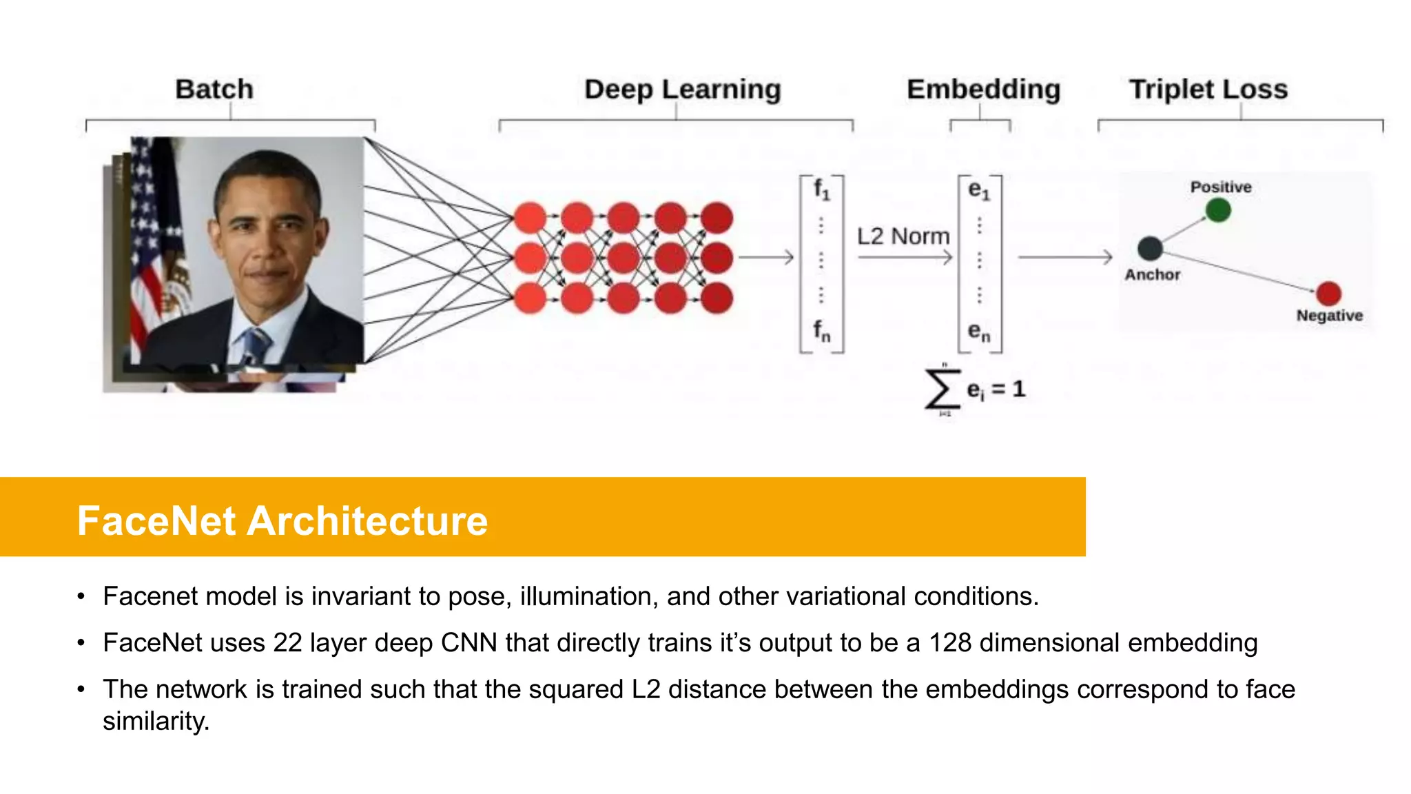
• FaceNet provides a unified embedding for face
recognition, verification and clustering tasks.
• Developed by Google Researchers - Schroff et al. at
Google in their 2015 paper
• FaceNet learns a mapping from face images to a
compact Euclidean space where distances directly
correspond to a measure of face similarity.
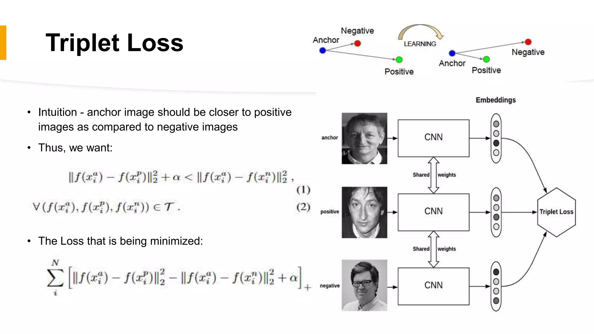
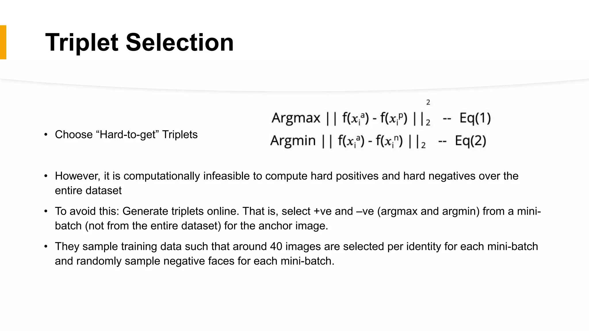
• A deep CNN is trained to optimize the embedding itself
using a novel online triplet mining method.
• These face embeddings achieved state-of-the-art
results on standard face recognition benchmark
datasets (cuts the error rate in comparison to the best
published result [2015] by 30%

5. FaceNet Architecture
• Facenet model is invariant to pose, illumination, and other variational conditions.
• FaceNet uses 22 layer deep CNN that directly trains it’s output to be a 128 dimensional embedding
• The network is trained such that the squared L2 distance between the embeddings correspond to face
similarity.

6. Triplet Loss
• Intuition - anchor image should be closer to positive
images as compared to negative images
• Thus, we want:
• The Loss that is being minimized:

7. Triplet Selection
• Choose “Hard-to-get” Triplets
• However, it is computationally infeasible to compute hard positives and hard negatives over the
entire dataset
• To avoid this: Generate triplets online. That is, select +ve and –ve (argmax and argmin) from a mini-
batch (not from the entire dataset) for the anchor image.
• They sample training data such that around 40 images are selected per identity for each mini-batch
and randomly sample negative faces for each mini-batch.

8. Deep Convolutional Networks
• CNN is trained using Stochastic Gradient Descent (SGD) with standard backprop and
AdaGrad.
• The inventors of Facenet explored 2 types of architecture where the difference is in the no.
of parameters and FLOPS
• Model1 – uses the Zeiler&Fergus architecture and results in a model 22 layers deep. It has
a total of 140million parameters and requires around 1.6 billion FLOPS per image.
• Model2 - based on GoogLeNet style Inception models which has 20× fewer parameters
(around 6.6M-7.5M) and up to 5×fewer FLOPS(between 500M-1.6B).

9. Zeiler&Fergus-
Inspired Architecture
• Consists of multiple interleaved layers of
convolutions, non-linear activations, local
response normalizations, and max
pooling layers (with several additional
1x1xd convolutional layers throughout).
• 1x1 conv layer is inspired by the cross-
channel parametric pooling

10. Inception-Inspired
Architecture

11. Dataset and Evaluation
• The model is evaluated on 4 different datasets & these parameters are
evaluated:
1. Hold-out Test Set: 1M images having the same distribution as the training set. Divided into 5
subsets. VAL and FAR are calculated on 100k x 100k image pairs.
2. Personal Photos: 12k images with FAR and VAL calculated for 12k x 12k image pairs.
3. Labeled Faces in the Wild (LFW): de-facto academic test set for face recognition. FAR and
VAL are not calculated.
4. Youtube Faces DB: setup is similar to LFW, but pairs of videos instead of images are used.
FAR and VAL are not calculated.

12. Experiments with Facenet
Accuracy on Different Models
Embedding
Dimensionality
JPEG
compression
Image Size

13. Performance on LFW
• Achieved record breaking classification accuracy of 99.63%
• This reduces the error reported for DeepFace by more than a factor of 7
• This is the performance of model NN1, but even the much smaller NN3 achieves
performance that is not statistically significantly different.
• Classification accuracy achieved is 95.12% (state-of-the-art).
• Previous efforts DeepId2+ (Sun et al.) had achieved 93.2%
Performance Youtube Faces DB

14. Face Clustering
• These embedding can be used to cluster a users
personal photos into groups of people withthe same
identity
• Figure shows one cluster in a users personal photo
collection, generated using agglomerative clustering.
• It is a clear showcase of the incredible invariance to
occlusion, lighting, pose and even age

15. How to Apply Facenet
Create a folder with images
(>1) per person. The images
should have fairly good
resolution and need not
necessarily be cropped
Images should be on
grayscale and scaled
accordingly
Use pre-trained models to
detect faces and create a
bounding box.
Train by passing cropped
images to facenet to learn
the embeddings.
For testing, pass a new
image which is not in our
database.
Compute the face
embedding using the same
network we used above and
then compare this
embedding with the rest of
the embeddings we have.

16. Summary and Conclusions
• state-of-the-art face recognition performance using only 128-bytes per
face.
• Minimal alignment required on the input dataset (tight crop around the
face area), unlike DeepFace (FAIR) which performs 3D alignment.

17. Related works
• Y. Taigman, M. Yang, M. Ranzato, and L. Wolf. Deepface: Closing the
gap to human-level performance in face verification.
• Y. Sun, X. Wang, and X. Tang. Deeply learned face representations are
sparse, selective, and robust.

18. Appendix

19. Computation vs.
Accuracy Trade-off
• 100M - 200M images training face thumbnails, having 8M identities are used
• Pre-processing: detecting faces and generating a tight bound box around each face. Resized depending on
the input sizes of the networks varying from 96x96 to 224x224.
• The graph shows a strong correlation between FLOPS & accuracy achieved. There isn’t a correlation b/w
accuracy vs no. of parameters.
• NN1 and NN2 differ in number of parameters by a factor of
20. But they achieve comparable performance
• NNS2, a tiny version of NN2, can be run on a mobile phone

20. Sensitivity to Image Quality
Their models are robust to JPEG
compression and perform well even
at a JPEG quality of 20
Performance drop is very less with
120x120 input image size and remains
acceptable even at 80x80

21. Embedding Dimensionality
• They experimented with a lot of dimensionalities
and chose 128-D, as it was the best performing.
• It was expected that the larger dimensionalities
would perform better, but it could also mean that
they require more training.
• Smaller embedding dimensions could be
employed on mobile devices, with minor loss of
accuracy.

22. Amount of Training Data
• Smaller model with input size
of 96x96 was employed for
this analysis. It has same
architecture as NN2 but
without the 5x5 conv. in the
inception module.