Download to read offline
![Exact Differential Equation:
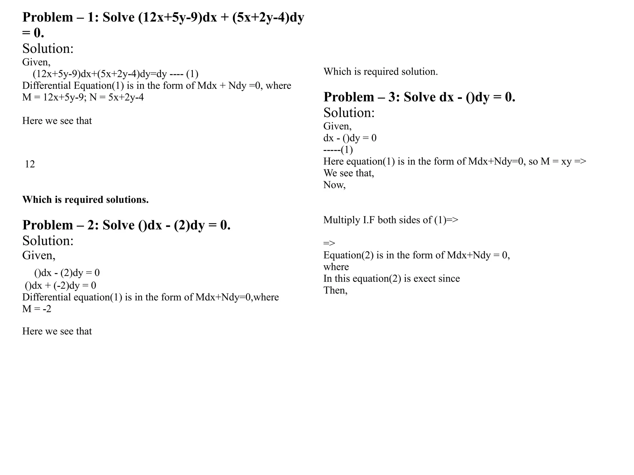
Problem – 1: Solve = 0.
Solution:
Given,
= 0 ----(1)
Equation(1) is in the form of
Here,
Hence, equation(1) is exact as
Then,
Which is required Solution. Ref: Simmons, G. F. (1991).
Differential equations with applications and historical notes (2nd
ed., p. 126). McGraw-Hill.
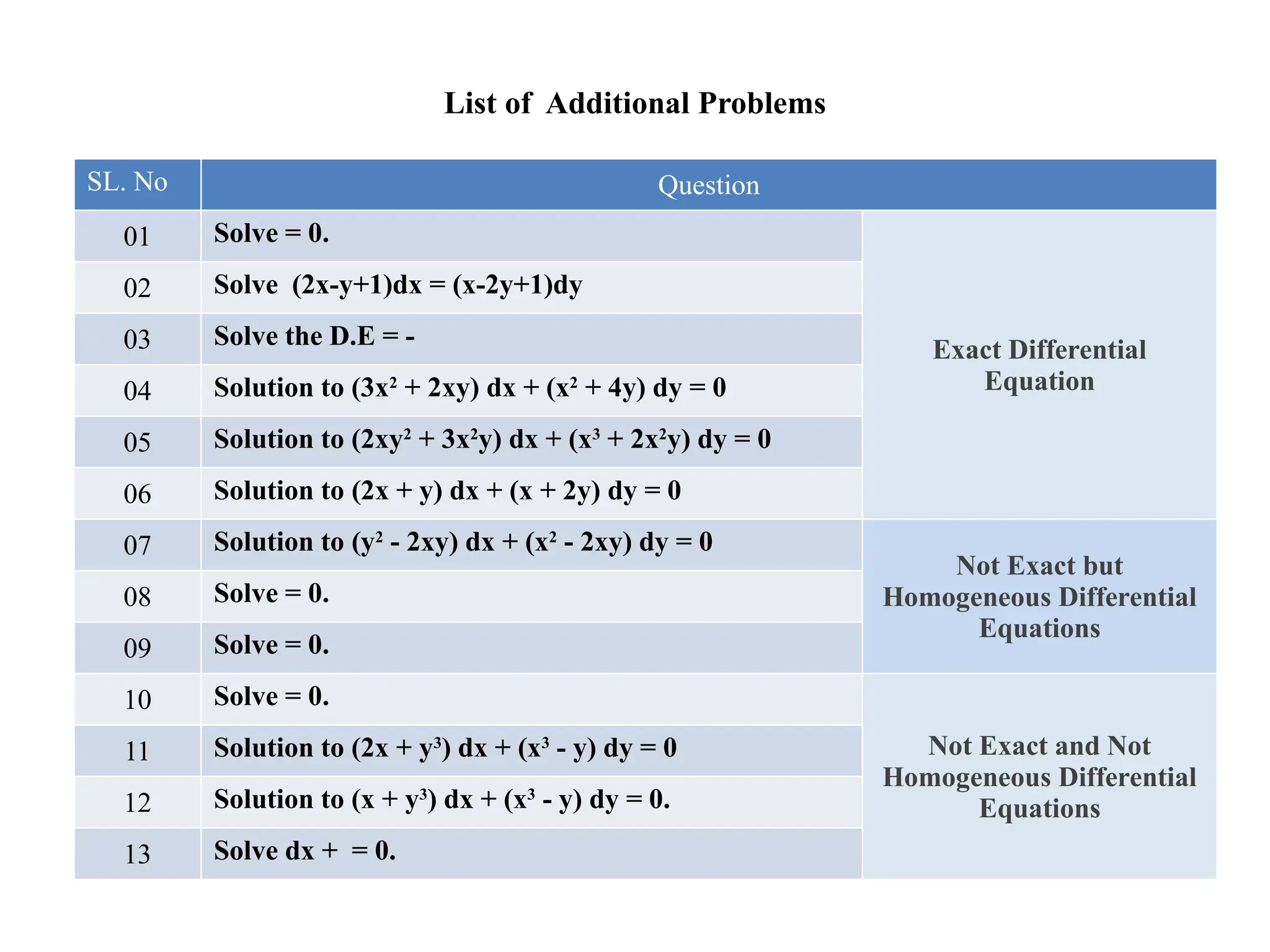
Problem-2: Solve (2x-y+1)dx = (x-2y+1)dy
Solution:
Given, D.E. VS
(2x-y+1)dx = (x-2y+1)dy
(2x-y+1)dx – (x-2y+1)dy = 0
Compair it with Mdx+Ndy = 0
M = 2x-y+1, N= -x+2y-1
= 0-1+0, = -1+0+0
= -1, = -1
Since = = -1
the given D.E is exact the saln of given DE is given by mdx +
(term of N not containing x) dy = C
(2x-y+1)dx + (2y-1)dy = C
- xy +1+ -y = C
- xy + x + - y = C
+ - xy + x – y = C
Which is required Solution.Ref: TIKLE'S ACADEMY OF MATHS(Jul
2, 2023), EXACT DIFFERENTIAL EQUATION SOLVED PROBLEM
6[video], https://www.youtube.com/watch?v=K-jYhSc_tpk
Problem-3: Solve the D.E = -
Solution:
Given D.E is
= -
-(2+) dy = dx
dx + (2+)dy=0
Compir it with mdx+ndy=0
M= , N= 2+
= 2xy, = 2xy
Since =
The given D.E is exact
The soln
of given D.E is give by,
Which is the required Solution. Ref: Ref: TIKLE'S ACADEMY OF
MATHS(Jul 2, 2023), EXACT DIFFERENTIAL EQUATION SOLVED
PROBLEM 6[video], https://www.youtube.com/watch?v=K-jYhSc_tpk](https://image.slidesharecdn.com/exectdifferentialeqn-241225201302-c31621bf/75/Exact-Differential-Equations-Theory-History-and-Real-Life-Application-13-2048.jpg)
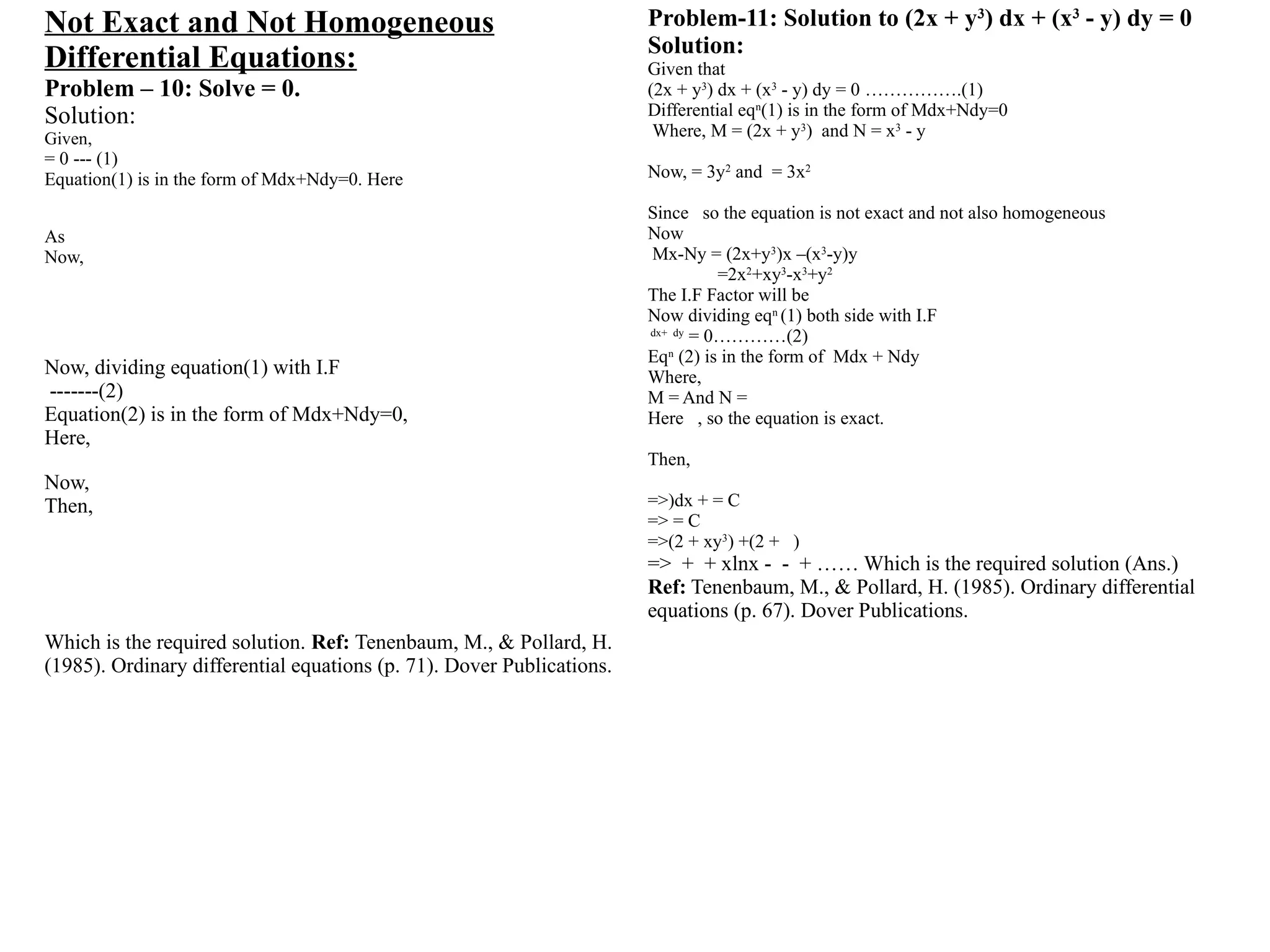
![Problem-12: Solution to (x + y3
) dx + (x3
- y) dy = 0.
Solution:
Given that
(x + y3
) dx + (x3
- y) dy = 0 …………….(1)
Differential eqn
(1) is in the form of Mdx+Ndy=0
Where, M = (x + y3
) and N = x3
- y
Now, = 3y2
and = 3x2
Since so the equation is not exact and not also homogeneous
Now
Mx-Ny = (x+y3
)x –(x3
-y)y
=x2
+xy3
-x3
+y2
The I.F Factor will be
Now dividing eqn
(1) both side with I.F
dx+ dy
= 0…………(2)
Eqn
(2) is in the form of Mdx + Ndy
Where,
M = And N =
Here , so the equation is exact.
Then,
=>)dx + = C
=> = C
=>( + xy3
) +( + )
=> + + xlnx - - + …… Which is the required solution (Ans.) Ref:
Tenenbaum, M., & Pollard, H. (1985). Ordinary differential equations (p.
68). Dover Publications.
Problem-13: Solve dx + = 0.
Solution:
Given D.E
dx + = 0
Compare it with mdx+ndy=0
M= , N= =0
M= , N=
M= + N= -
M= 2x+ , N= -
,
Here,
The given D.E is Exact
The soln
is given by,
Which is the required Solution.
Ref: TIKLE'S ACADEMY OF MATHS(Jul 2, 2023), EXACT
DIFFERENTIAL EQUATION SOLVED PROBLEM 6[video],
https://www.youtube.com/watch?v=K-jYhSc_tpk](https://image.slidesharecdn.com/exectdifferentialeqn-241225201302-c31621bf/75/Exact-Differential-Equations-Theory-History-and-Real-Life-Application-18-2048.jpg)


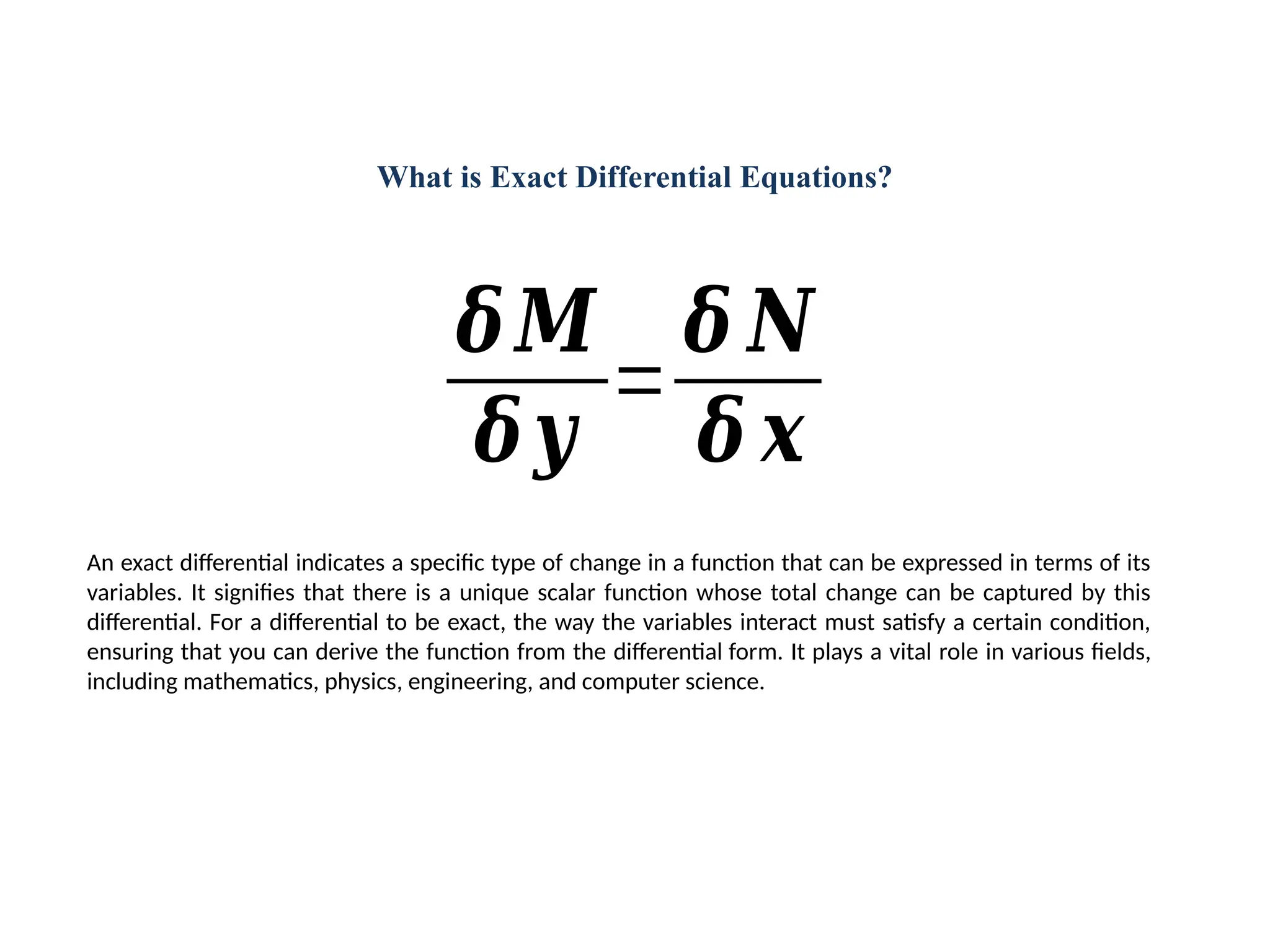
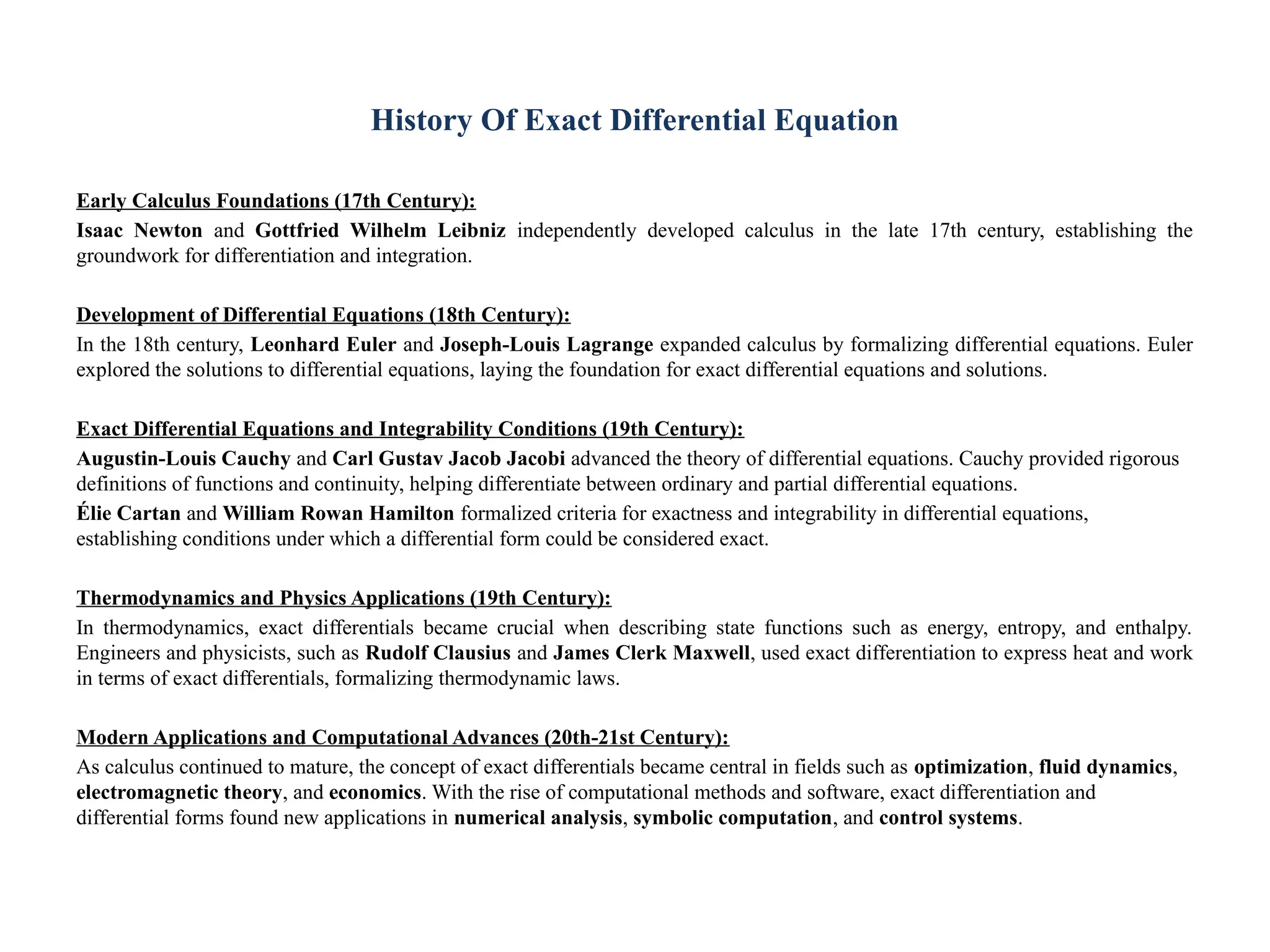
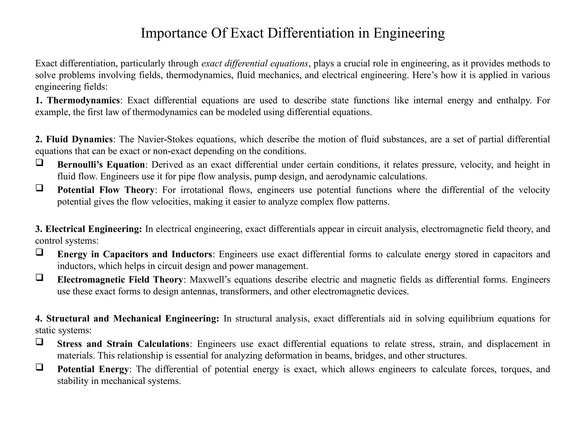
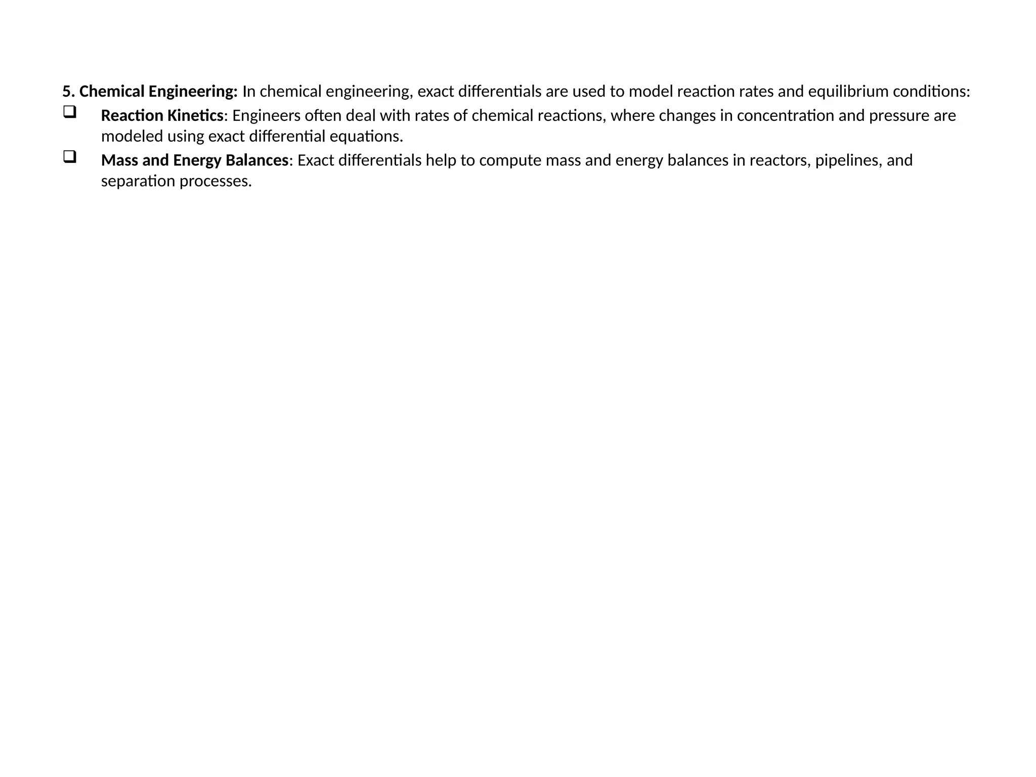
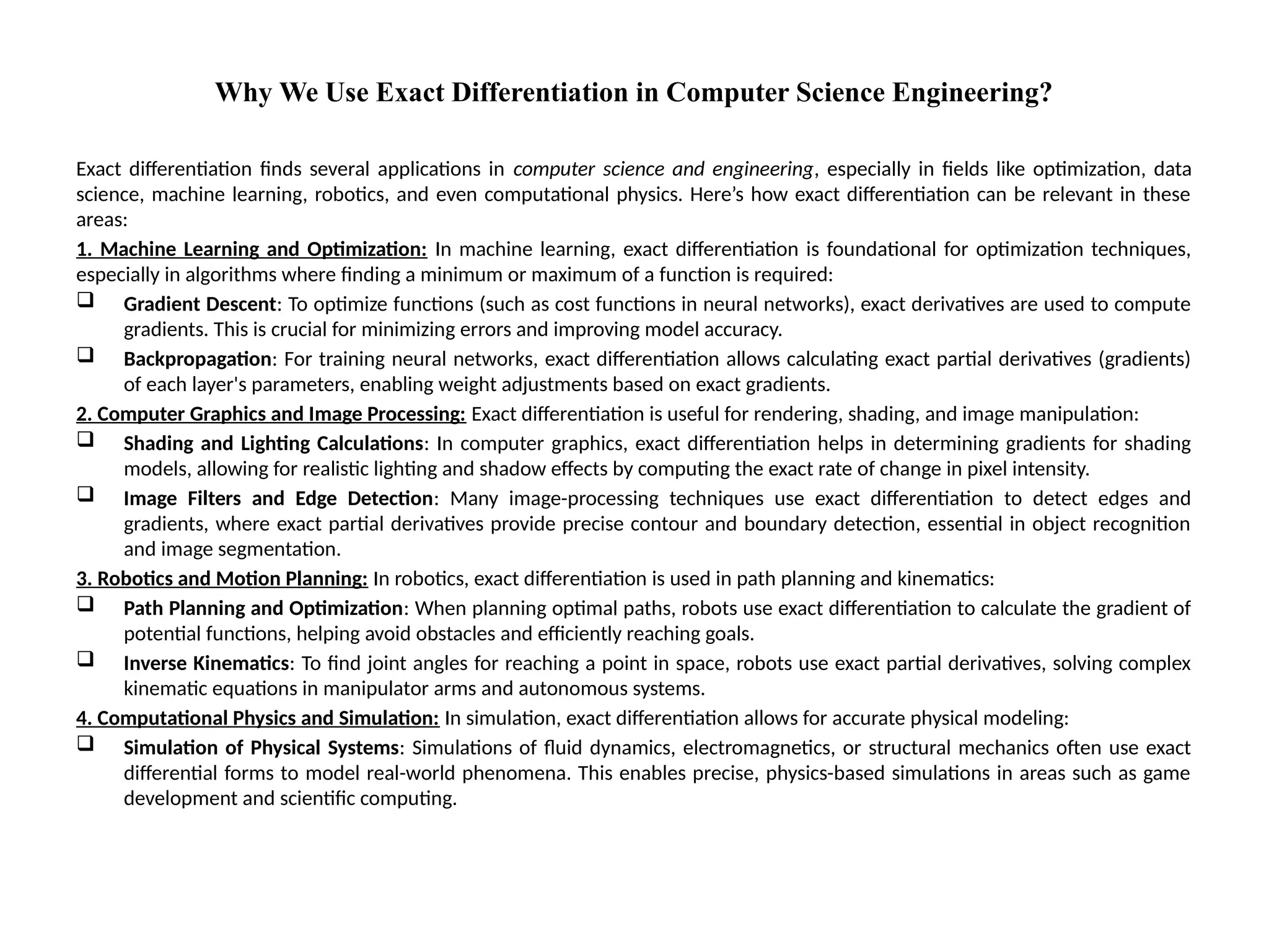
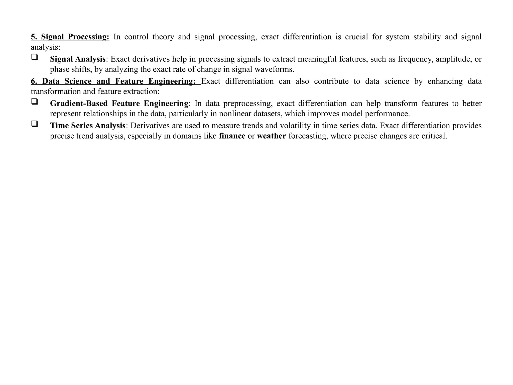
The document discusses exact differential equations, detailing their history, importance, and applications in various fields such as engineering and computer science. It covers the mathematical foundations laid by notable figures and examines specific case studies demonstrating the use of exact differentials in thermodynamics, fluid dynamics, and machine learning. It also provides problems and solutions related to exact differential equations, illustrating their practical relevance.


