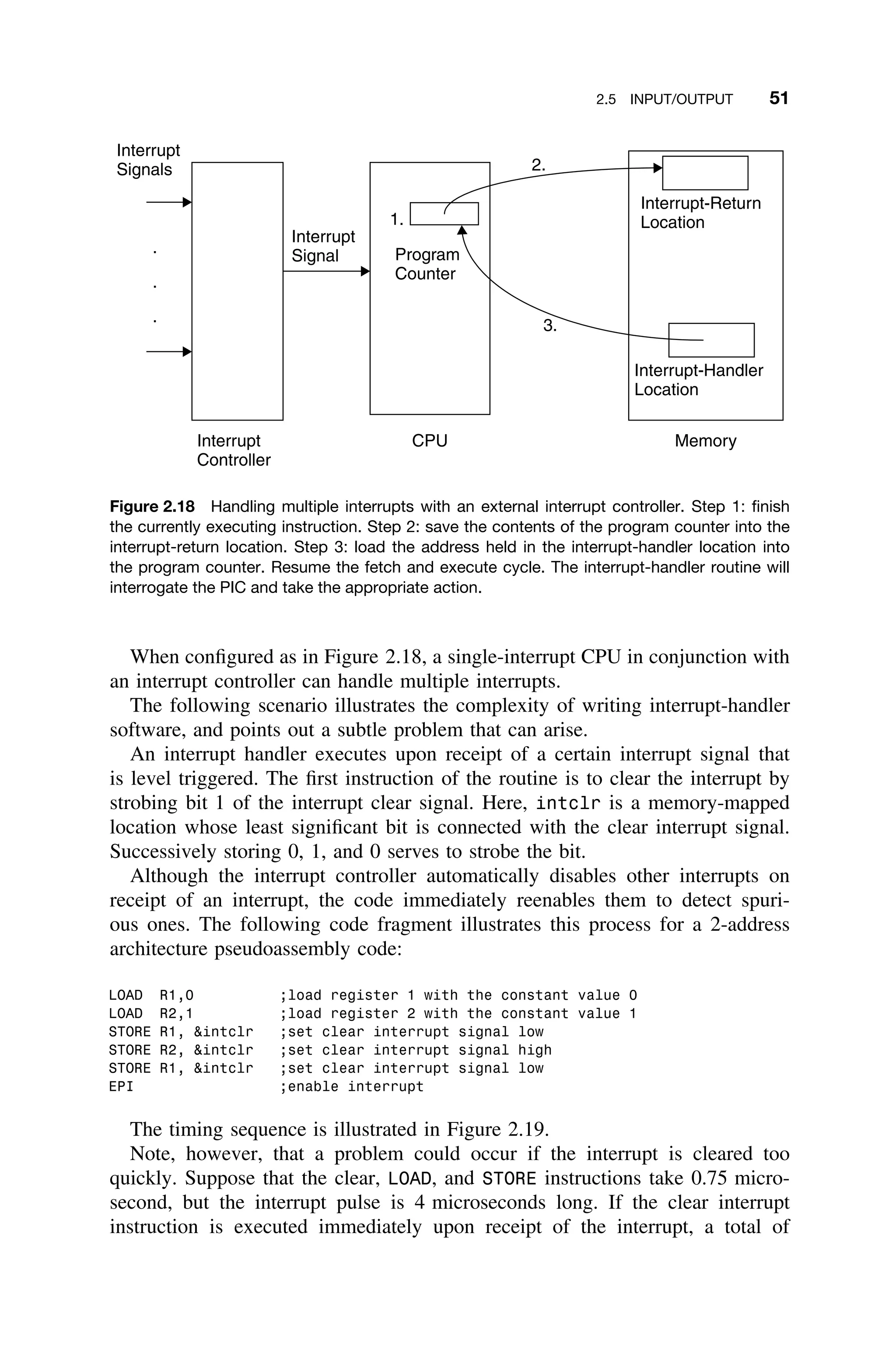
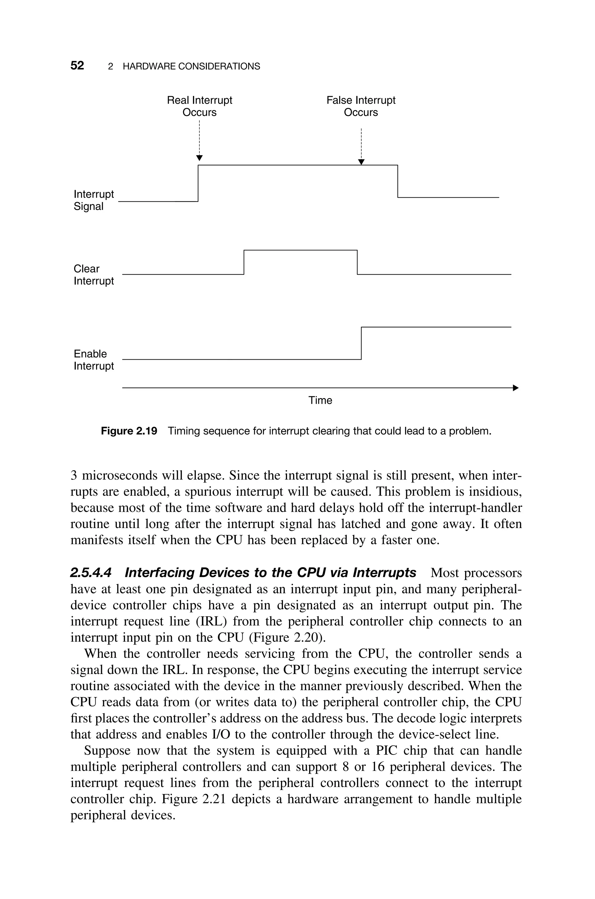
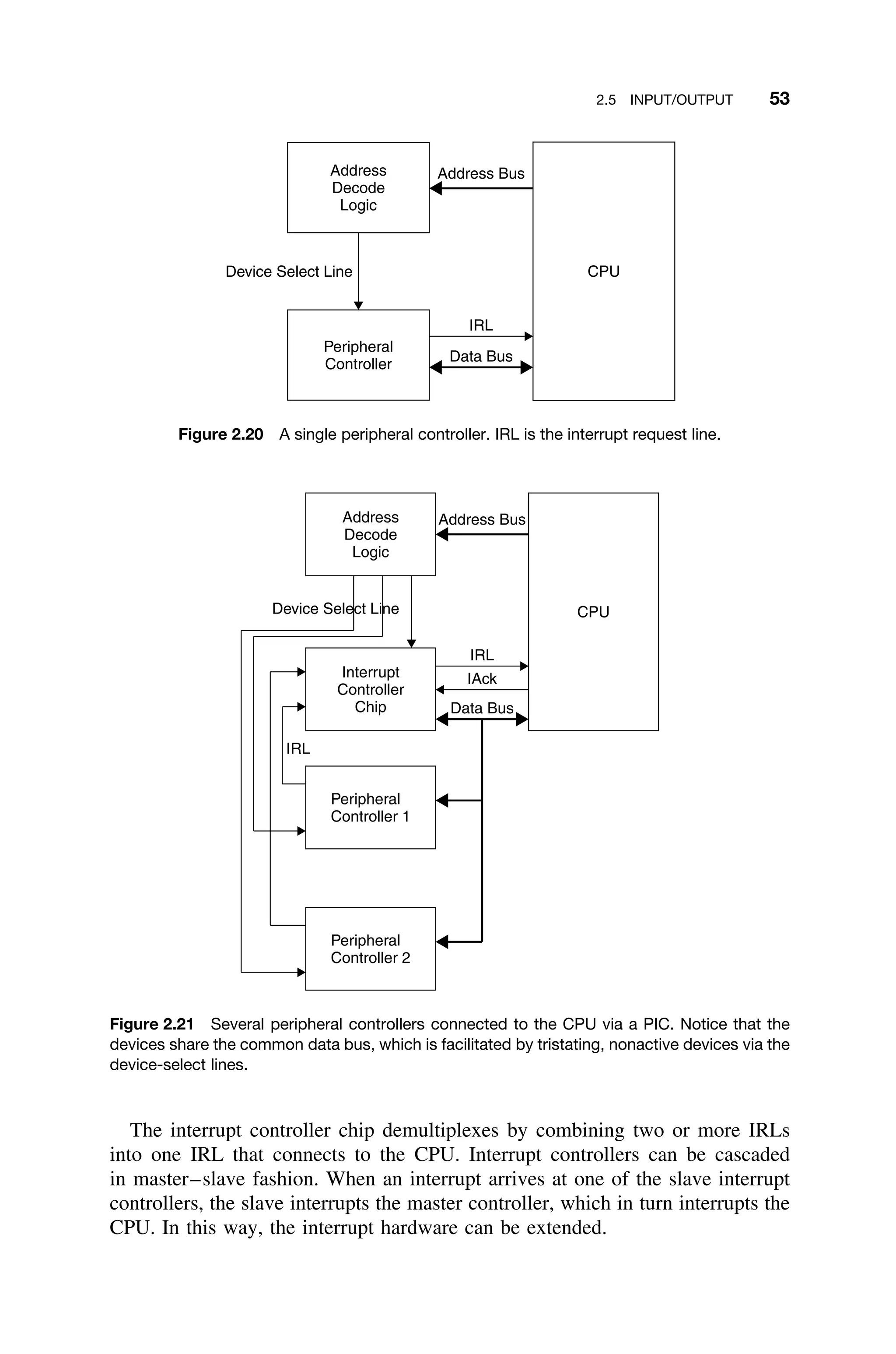
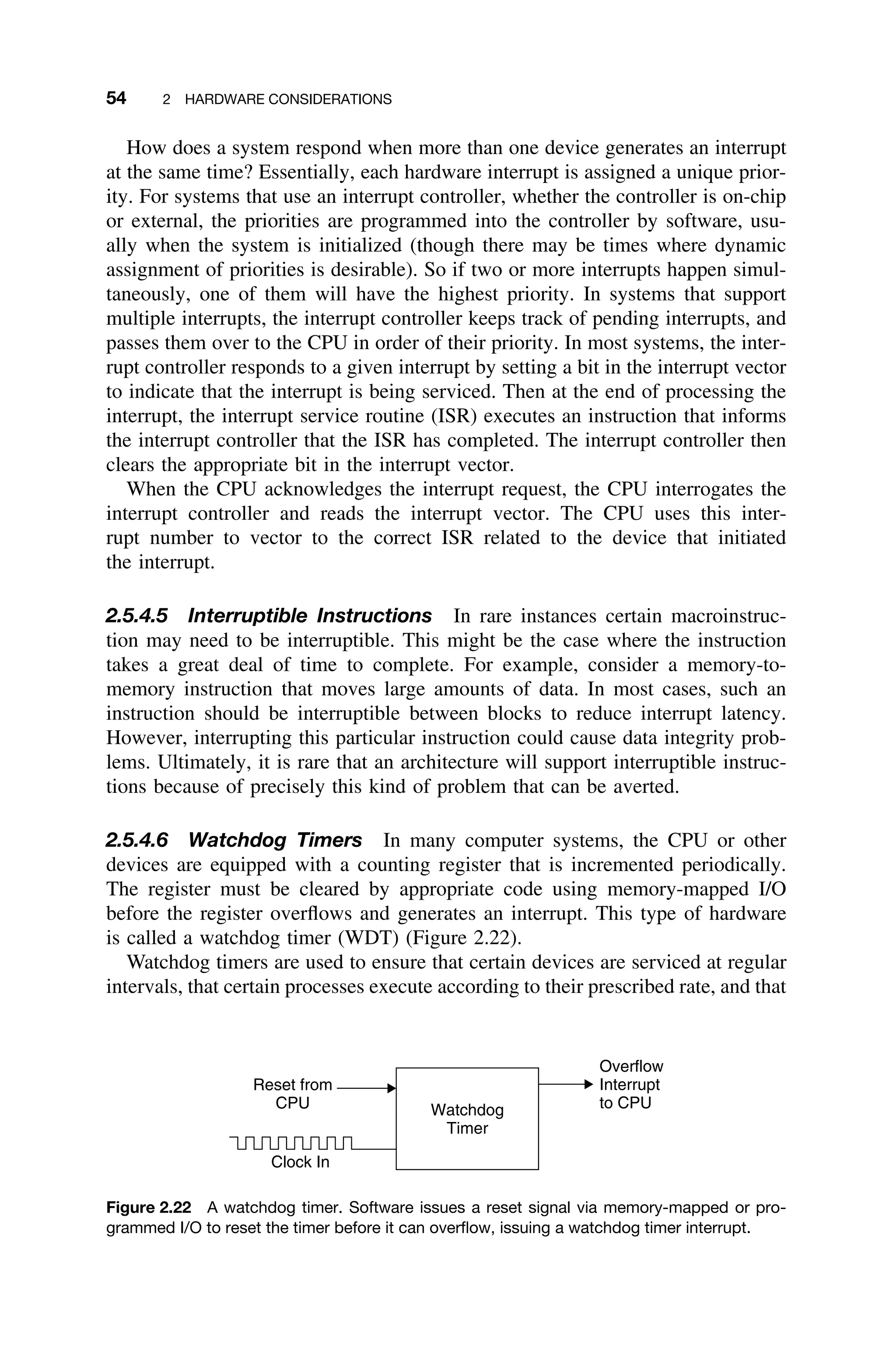
This document provides a summary of a book titled "Real-Time Systems Design and Analysis". It includes information about the publisher, IEEE Press, as well as the editorial board for IEEE Press. It also lists the author of the third edition of the book as Phillip A. Laplante and provides basic copyright information.


![xviii PREFACE TO THE THIRD EDITION
advanced reader, such as one by the author [Laplante00]. This book is especially
useful in an industrial setting for new real-time systems designers who need to
get “up to speed” very quickly. This author has used earlier editions of this book
in this way to teach short courses for several clients.
The reader is assumed to have some experience in programming in one of the
more popular languages, but other than this, the prerequisites for this text are
minimal. Some familiarity with discrete mathematics is helpful in understanding
some of the formalizations, but it is not essential. A background in basic calculus
and probability theory will assist in the reading of Chapter 7.
PROGRAMMING LANGUAGES
Although there are certain “preferred” languages for real-time system design,
such as C, C++, Ada 95, and increasingly Java, many real-time systems are still
written in Fortran, assembly language, and even Visual BASIC. It would be unjust
to focus this book on one language, say C, when the theory should be language
independent. However, for uniformity of discussion, points are illustrated, as
appropriate, in generic assembly language and C. While the C code is not intended
to be ready-to-use, it can be easily adapted with a little tweaking for use in a
real system.
ORGANIZATION OF THE BOOK
Real-time software designers must be familiar with computer architecture and
organization, operating systems, software engineering, programming languages,
and compiler theory. The text provides an overview of these subjects from the
perspective of the real-time systems designer. Because this is a staggering task,
depth is occasionally sacrificed for breadth. Again, suggestions for additional
readings are provided where depth has been sacrificed.
The book is organized into chapters that are essentially self-contained. Thus,
the material can be rearranged or omitted, depending on the background and inter-
ests of the audience or instructor. Each chapter contains both easy and challenging
exercises that stimulate the reader to confront actual problems. The exercises,
however, cannot serve as a substitute for practical experience.
The first chapter provides an overview of the nature of real-time systems. Much
of the basic vocabulary relating to real-time systems is developed along with a
discussion of the challenges facing the real-time system designer. Finally, a brief
historical review is given. The purpose of this chapter is to foreshadow the rest
of the book as well as quickly acquaint the reader with pertinent terminology.
The second chapter presents a more detailed review of basic computer archi-
tecture concepts from the perspective of the real-time systems designer and some
basic concepts of electronics. Specifically, the impact of different architectural
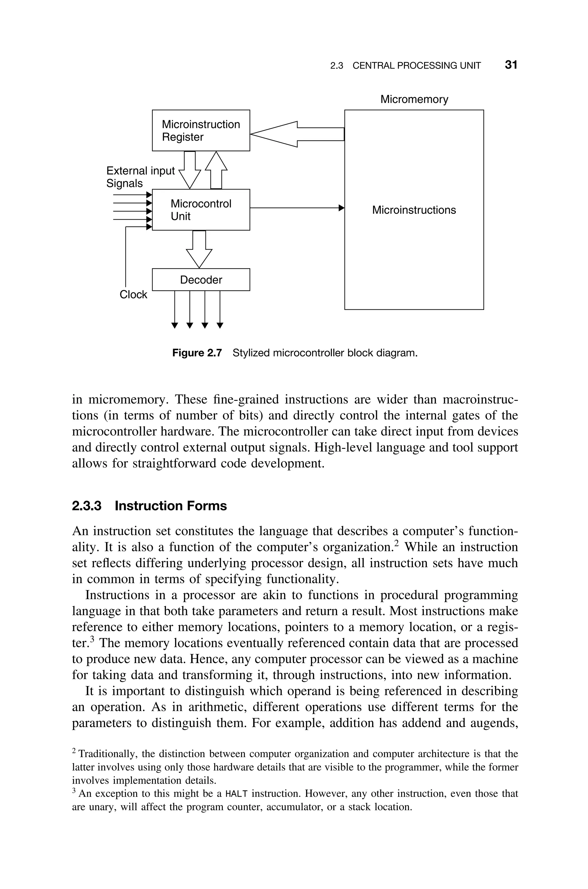
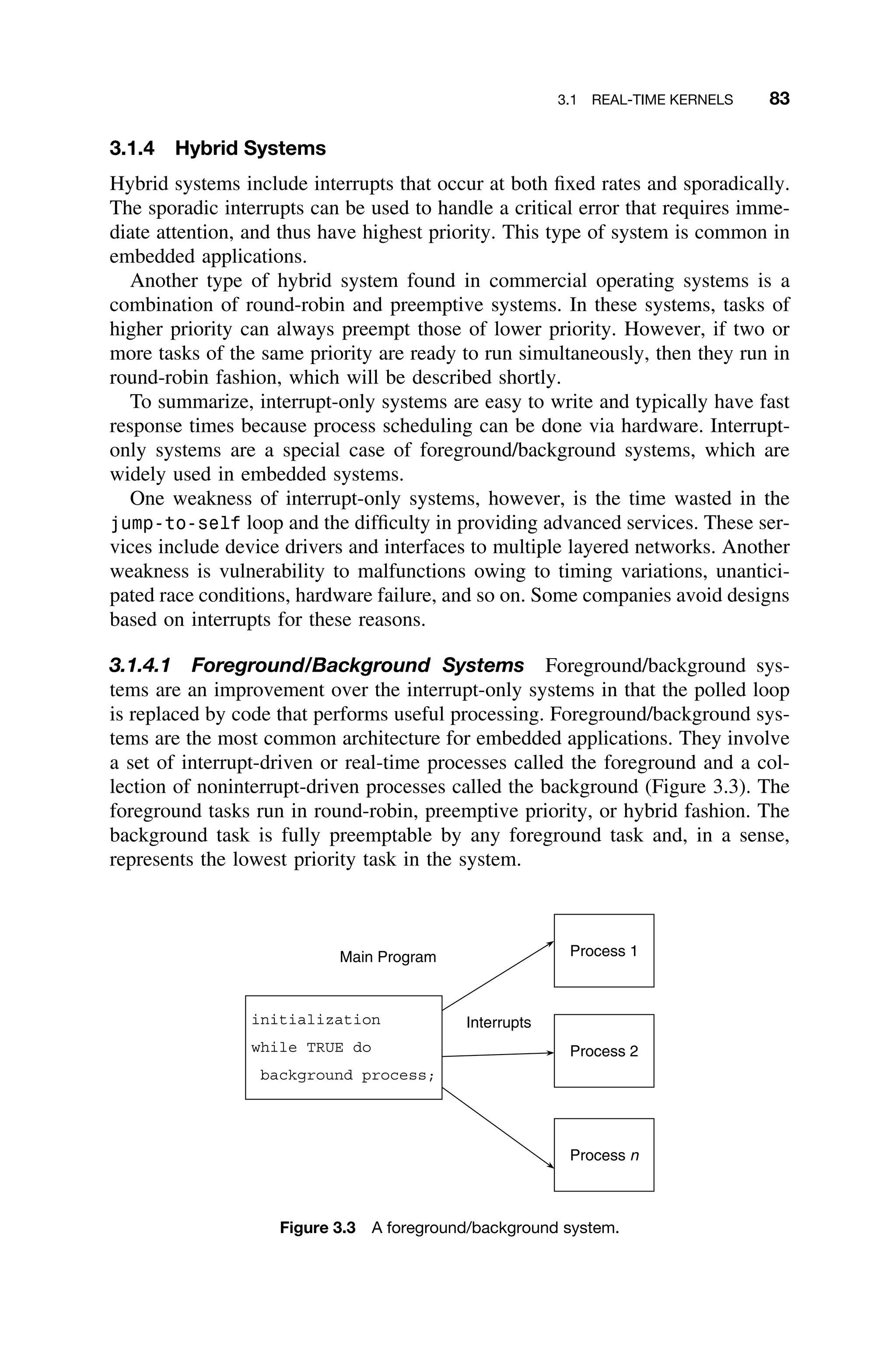
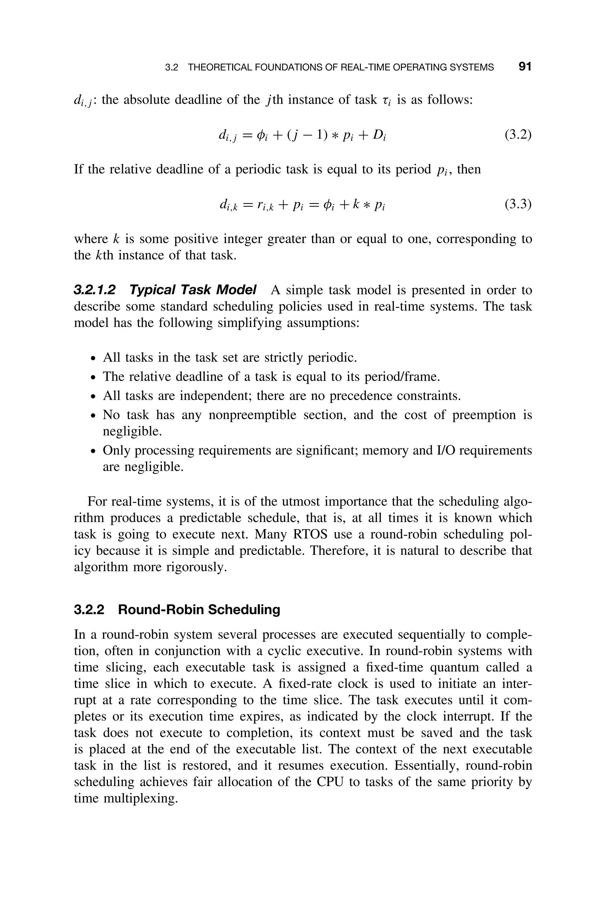
features on real-time performance is discussed. The remainder of the chapter](https://image.slidesharecdn.com/epdf-230618090952-bdcb6616/75/epdf-pub_real-time-systems-design-and-analysis-pdf-19-2048.jpg)
![xx PREFACE TO THE THIRD EDITION
such a game or simulation, using at least the coroutine model. The application
should be useful or at least pleasing, so some sort of a game is a good choice. The
project should take no more than 15 hours and cover all phases of the software
life-cycle model discussed in the text. Hence, those readers who have never built
a real-time system will have the benefit of the experience.
A NOTE ON REFERENCES
Real-Time Systems Engineering is based on more than 50 years of experience and
work by many individuals. Rather than clutter the text with endless citations for
the origin of each idea, the author chose to cite only the most key ideas where
the reader would want to seek out the source for further reading. Some of the text
is adapted from two other books written by the author on software engineering
and computer architecture [Laplante03c] [Gilreath03]. Where this has been done,
it is so noted. Note: In all cases where some sections of this text, particularly
the author’s own, appear as “adapted” or “paraphrased,” it means that the work
is being reprinted with both major and minor differences. However, rather than
confuse the issue with intermittent quotation marks for verbatim text, the reader
should attribute all ideas to cited authors from the point where the usage is
noted to the ending reference. This author, however, retains responsibility for
any errors. In all cases, permission to reprint this material has been obtained.
Many good theoretical treatments of real-time systems exist, and they are
noted where applicable. However, these books are sometimes too theoretical for
practicing software engineers and students who are often too impatient to wade
through the derivations for the resultant payoff. These readers want results that
they can use now in the trenches, and they want to see how they can be used,
not just know that they exist. In this text, an attempt is made to distill the best
of the theoretical results, combined with practical experience to provide a toolkit
for the real-time designer.
This book contains an extensive bibliography. Where verbatim phrases were
used or where a figure came from another source, the author tried to cite it
appropriately. However, if any sources were inadvertently overlooked, the author
wishes to correct the error. In addition, in a book of this magnitude and com-
plexity, errors are bound to occur. Please notify the author if you find any errors
of omission, commission, citation, and so on by email, at plaplante@psu.edu and
they will be corrected at the next possible opportunity.
ACKNOWLEDGMENTS
The author wishes to acknowledge and thank the many individuals who assisted in
the preparation of this book. Dr. Purnendu Sinha of Concordia University, wrote
much of Chapter 3 and various parts of other chapters relating to scheduling
theory, contributed many exercises, and classroom tested the material. Dr. Colin](https://image.slidesharecdn.com/epdf-230618090952-bdcb6616/75/epdf-pub_real-time-systems-design-and-analysis-pdf-21-2048.jpg)


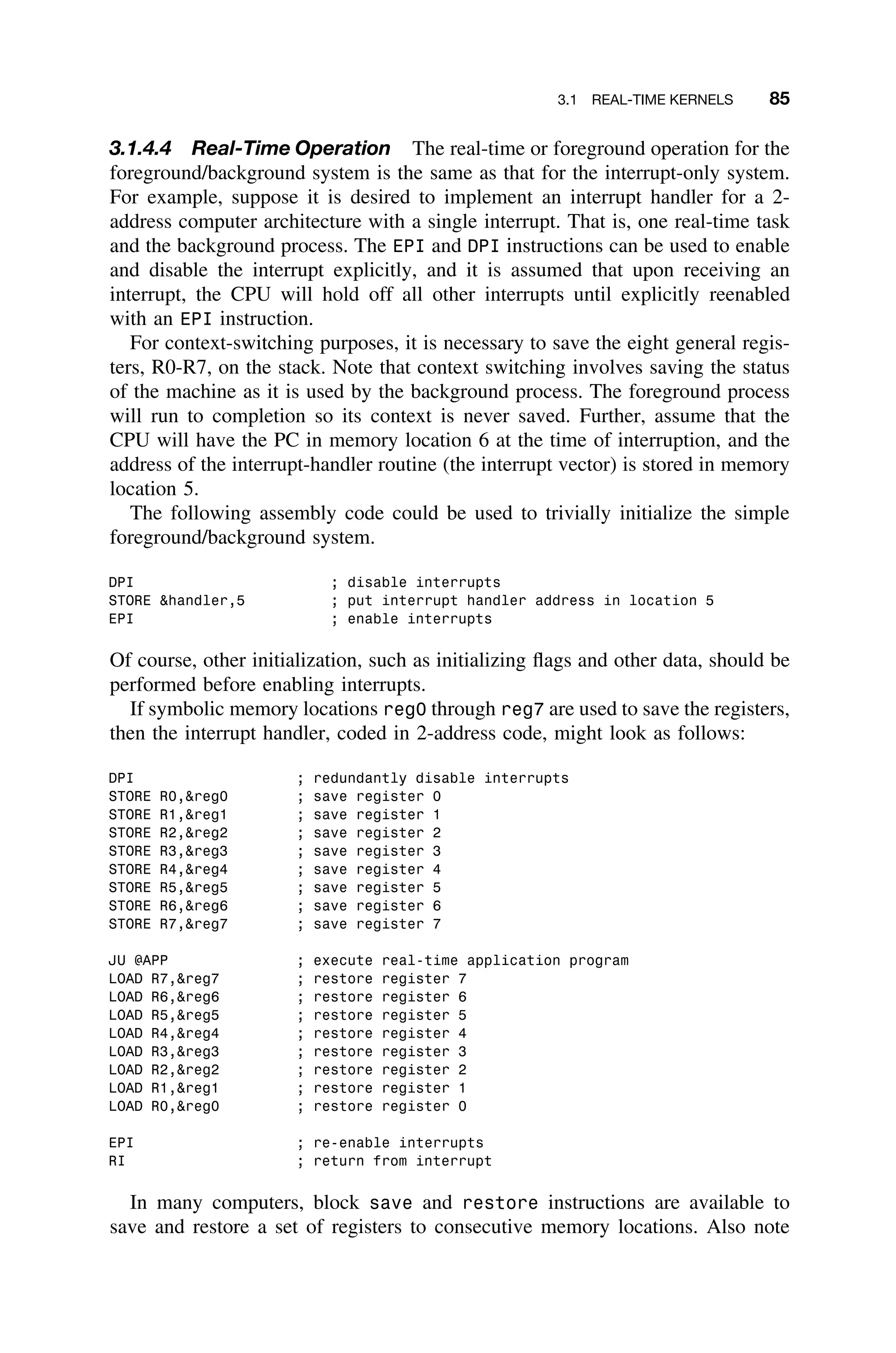
![1.1 TERMINOLOGY 3
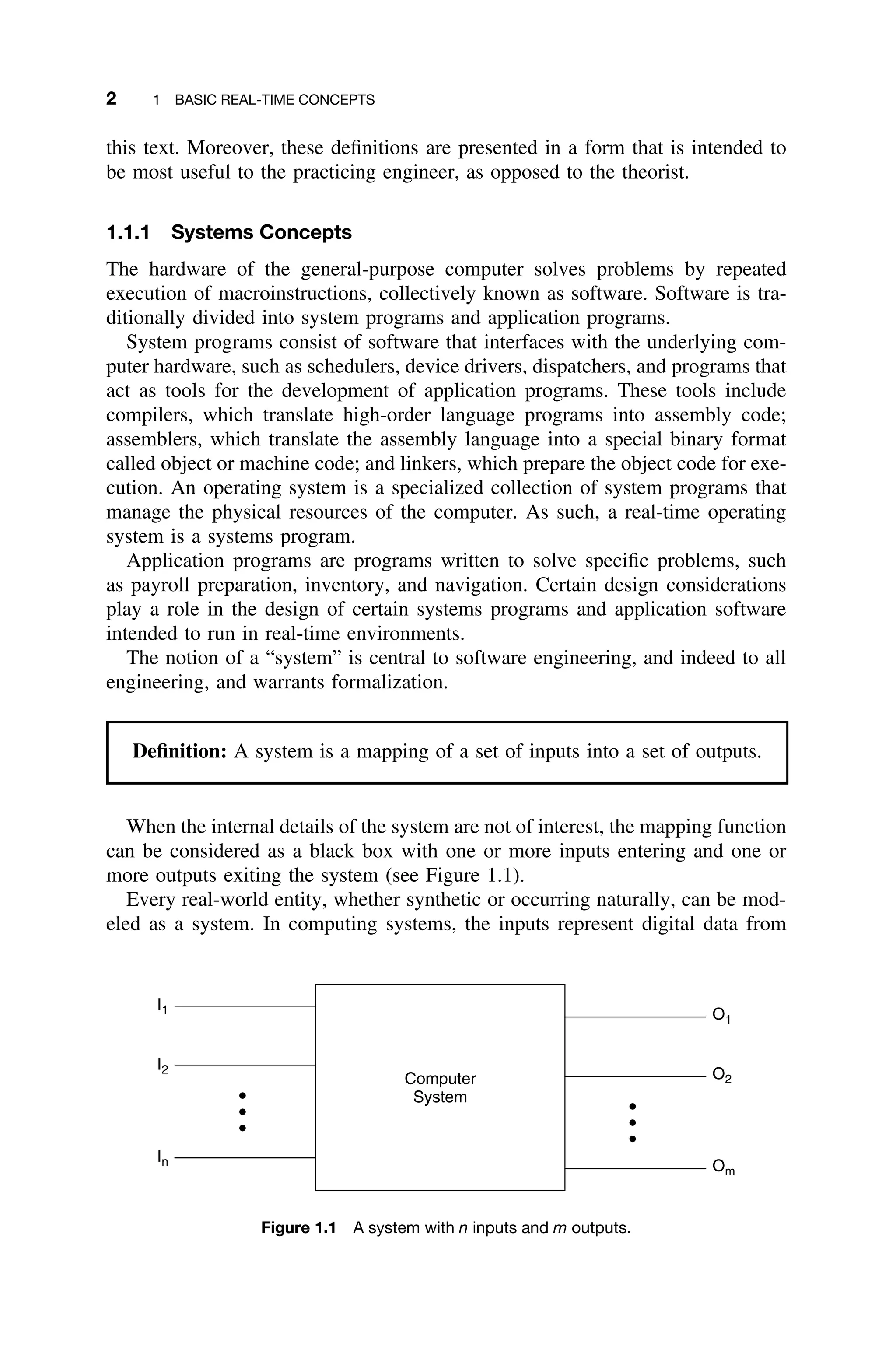
hardware devices and other software systems. The inputs are often associated
with sensors, cameras, and other devices that provide analog inputs, which are
converted to digital data, or provide direct digital input. The digital output of the
computer system can be converted to analog outputs to control external hardware
devices such as actuators and displays (Figure 1.2).
Modeling a real-time system, as in Figure 1.2, is somewhat different from
the more traditional model of the real-time system as a sequence of jobs to
be scheduled and performance to be predicted, which is very similar to that
shown in Figure 1.3. The latter view is simplistic in that it ignores the fact that
the input sources and hardware under control are complex. Moreover, there are
other, sweeping software engineering considerations that are hidden by the model
shown in Figure 1.3.
Computer
System
Sensor 1
Sensor 2
Sensor n
Display Data
Control Signal 1
Control Signal 2
Control Signal n
Camera Input
Figure 1.2 Typical real-time control system including inputs from sensors and imaging devices
and producing control signals and display information [Laplante03b].
Computer
System
Job 1
Job 2
Job n
Schedule
Figure 1.3 A classic representation of a real-time system as a sequence of jobs to be
scheduled.](https://image.slidesharecdn.com/epdf-230618090952-bdcb6616/75/epdf-pub_real-time-systems-design-and-analysis-pdf-26-2048.jpg)
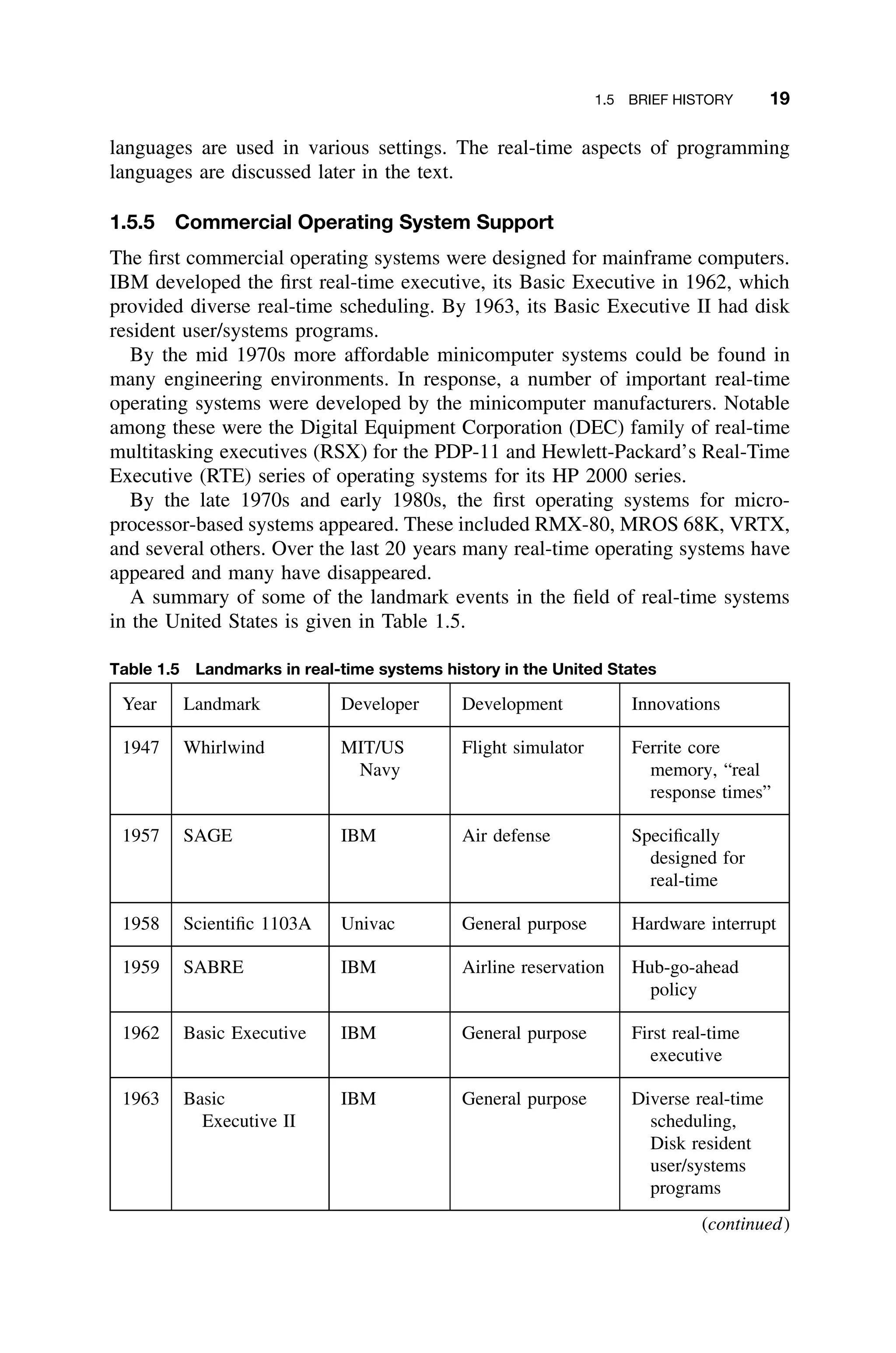
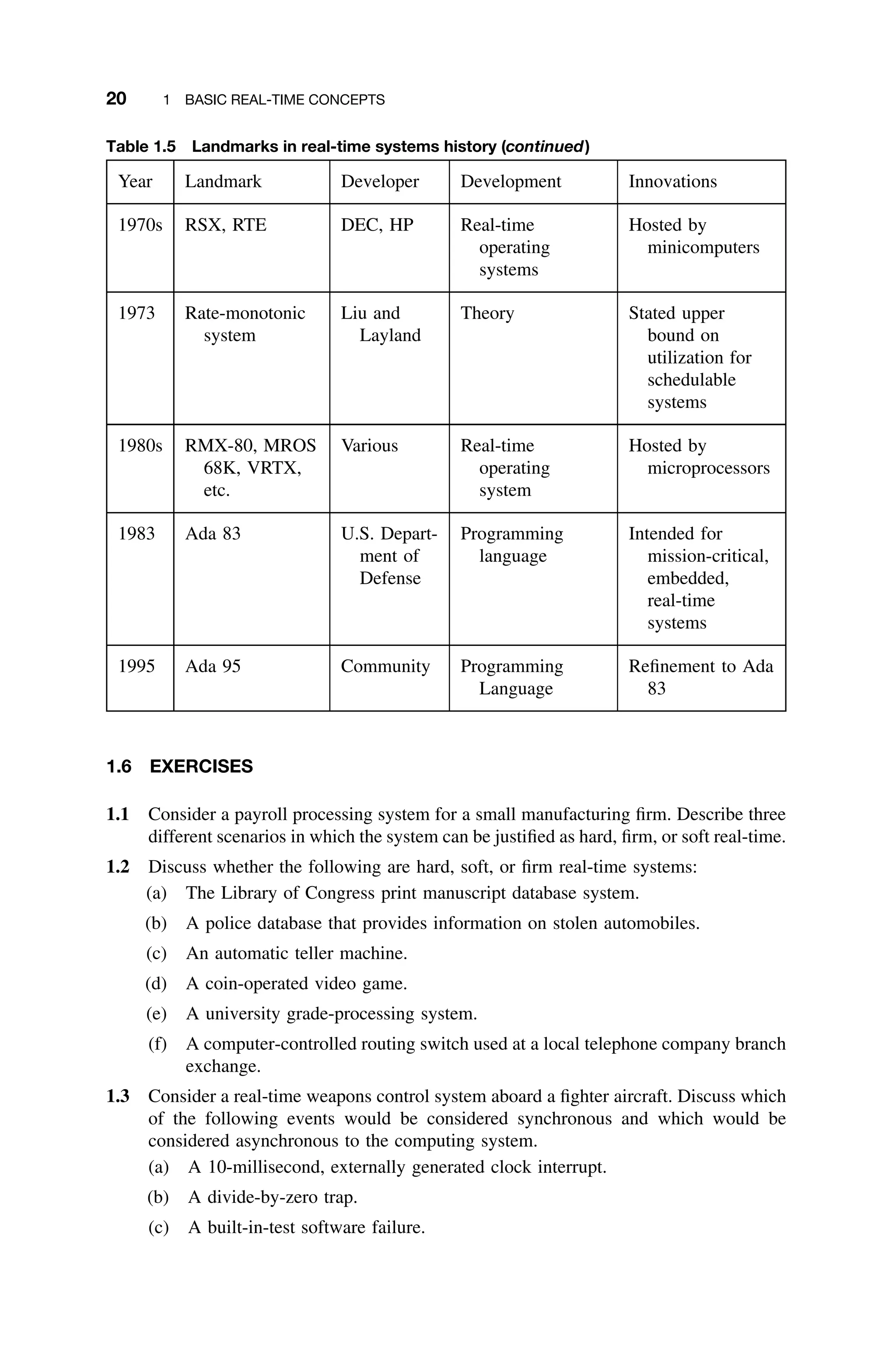
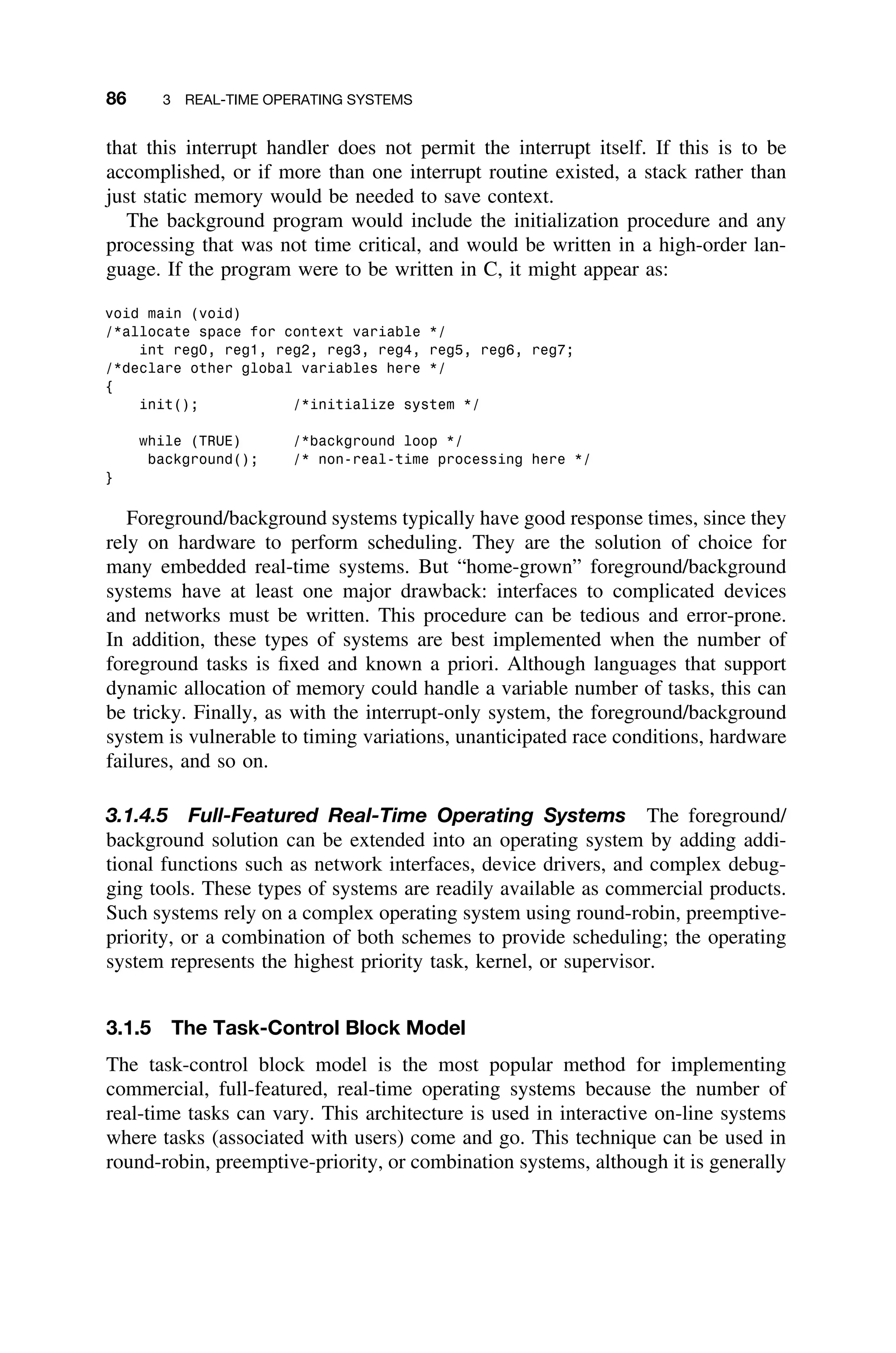
![1.5 BRIEF HISTORY 17
systems, or medical monitoring equipment, are complex, yet many still exhibit
characteristics of systems developed in the 1940s through the 1960s.
1.5.1 Theoretical Advances
Much of the theory of real-time systems is derived from the many underlying
disciplines shown in Figure 1.5. In particular, aspects of operations research,
which emerged in the late 1940s, and queuing systems, which emerged in the
early 1950s, have influenced most of the more theoretical results.
Martin published one of the earliest and certainly the most influential early
book on real-time systems [Martin67]. Martin’s book was soon followed by sev-
eral others (e.g., [Stimler695
]), and the influence of operations research (schedul-
ing) and queuing systems can be seen in these works. It is also interesting to
study these texts in the context of the limitations of the hardware of the time.
In 1973 Liu and Layland published their work on rate-monotonic theory
[Liu73]. Over the last 30 years significant refinement of this theory has made
it a more practical theory for use in designing real systems.
The 1980s and 1990s saw a proliferation of theoretical work on improv-
ing predictability and reliability of real-time systems and on solving problems
related to multiprocessing systems. Today, a rather limited group of experts con-
tinue to study issues of scheduling and performance analysis, even as a wider
group of generalist systems engineers tackle broader issues relating to the imple-
mentation of real, practical systems. An important paper by Stankovic et al.
[Stankovic95] described some of the difficulties in conducting research on real-
time systems – even with significant restriction of the system, most problems
relating to scheduling are too difficult to solve by analytic techniques.6
1.5.2 Early Systems
The origin of the term real-time computing is unclear. It was probably first
used either with project Whirlwind, a flight simulator developed by IBM for
the U.S. Navy in 1947, or with SAGE, the Semiautomatic Ground Environment
air defense system developed for the U.S. Air Force in the early 1950s. Both
projects qualify as real-time systems by today’s standards. In addition to its real-
time contributions, the Whirlwind project included the first use of ferrite core
memory and a form of high-order language compiler that predated Fortran.
Other early real-time systems were used for airline reservations, such as SABRE
(developed for American Airlines in 1959), as well as for process control, but the
advent of the national space program provided even greater opportunities for the
5
By coincidence, the author met Saul Stimler in 1995. He was still vibrant and actively thinking
about real-time systems.
6
At a 1992 NATO Advanced Study Institute that the author attended, Professor C. L. Liu (co-
discoverer of the rate-monotonic theory) stood up at a keynote talk and began by stating, “There are
no useful results in optimal scheduling for real-time systems.” The crowd was stunned (except the
author). There is no reason to believe that this situation has changed since then.](https://image.slidesharecdn.com/epdf-230618090952-bdcb6616/75/epdf-pub_real-time-systems-design-and-analysis-pdf-40-2048.jpg)

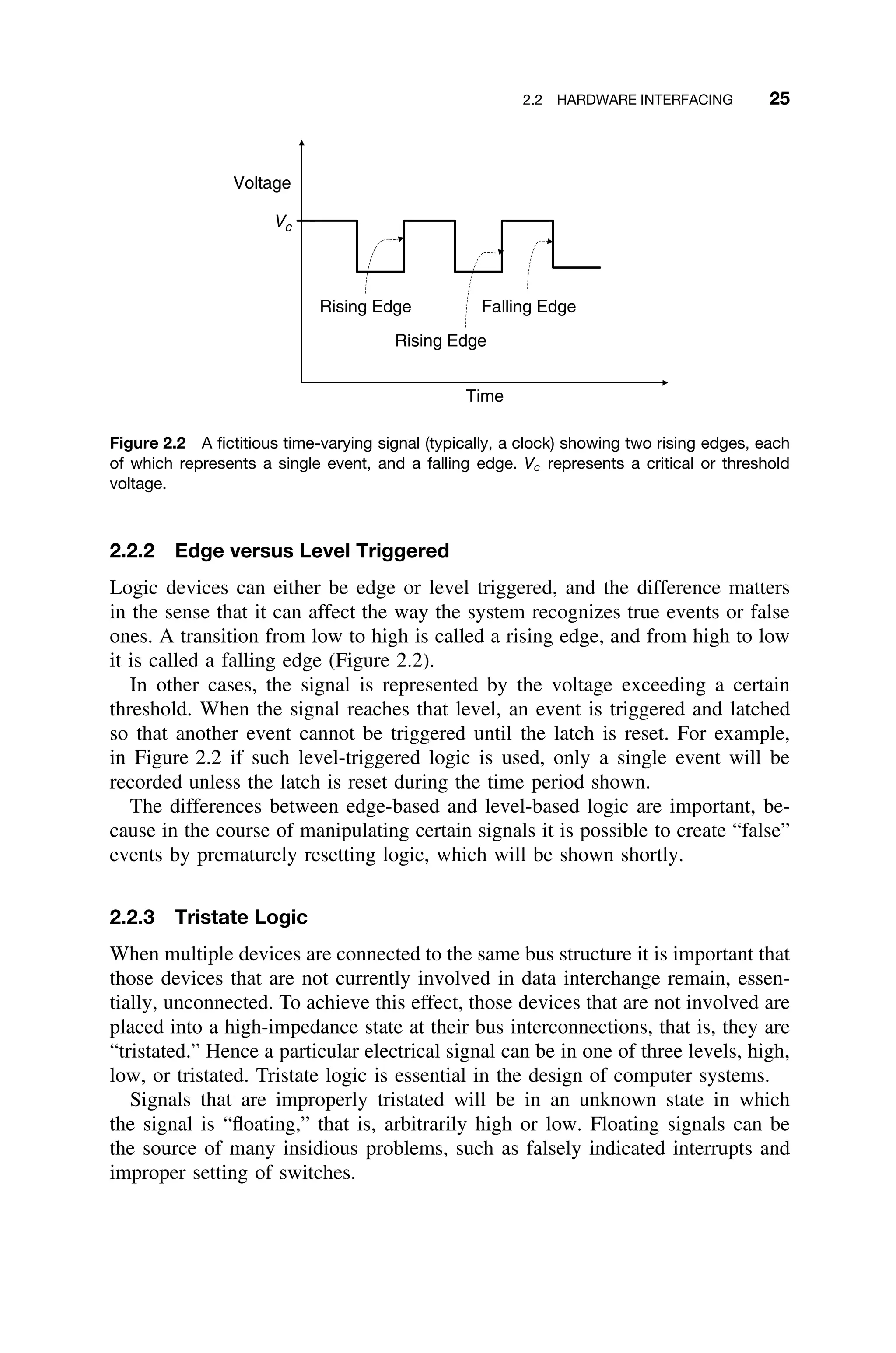
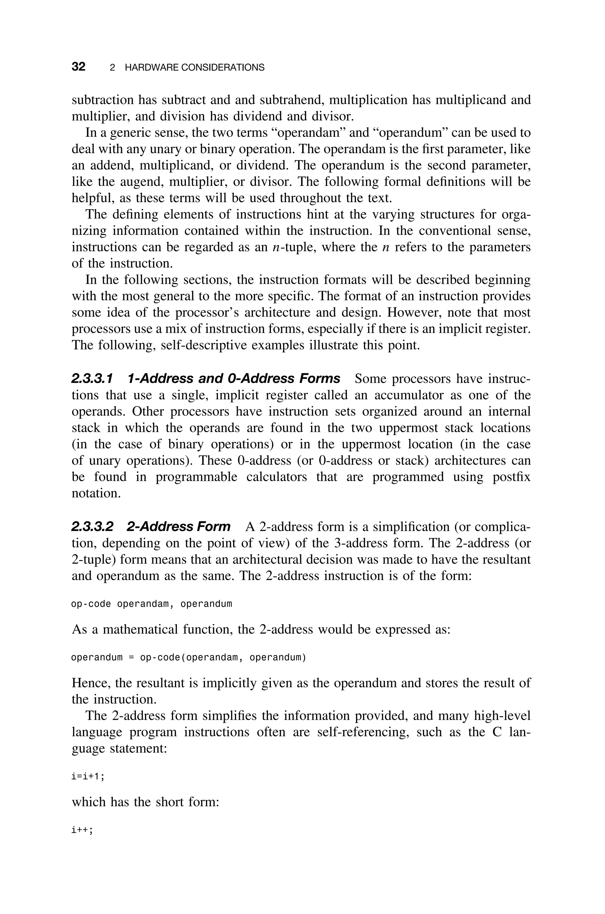
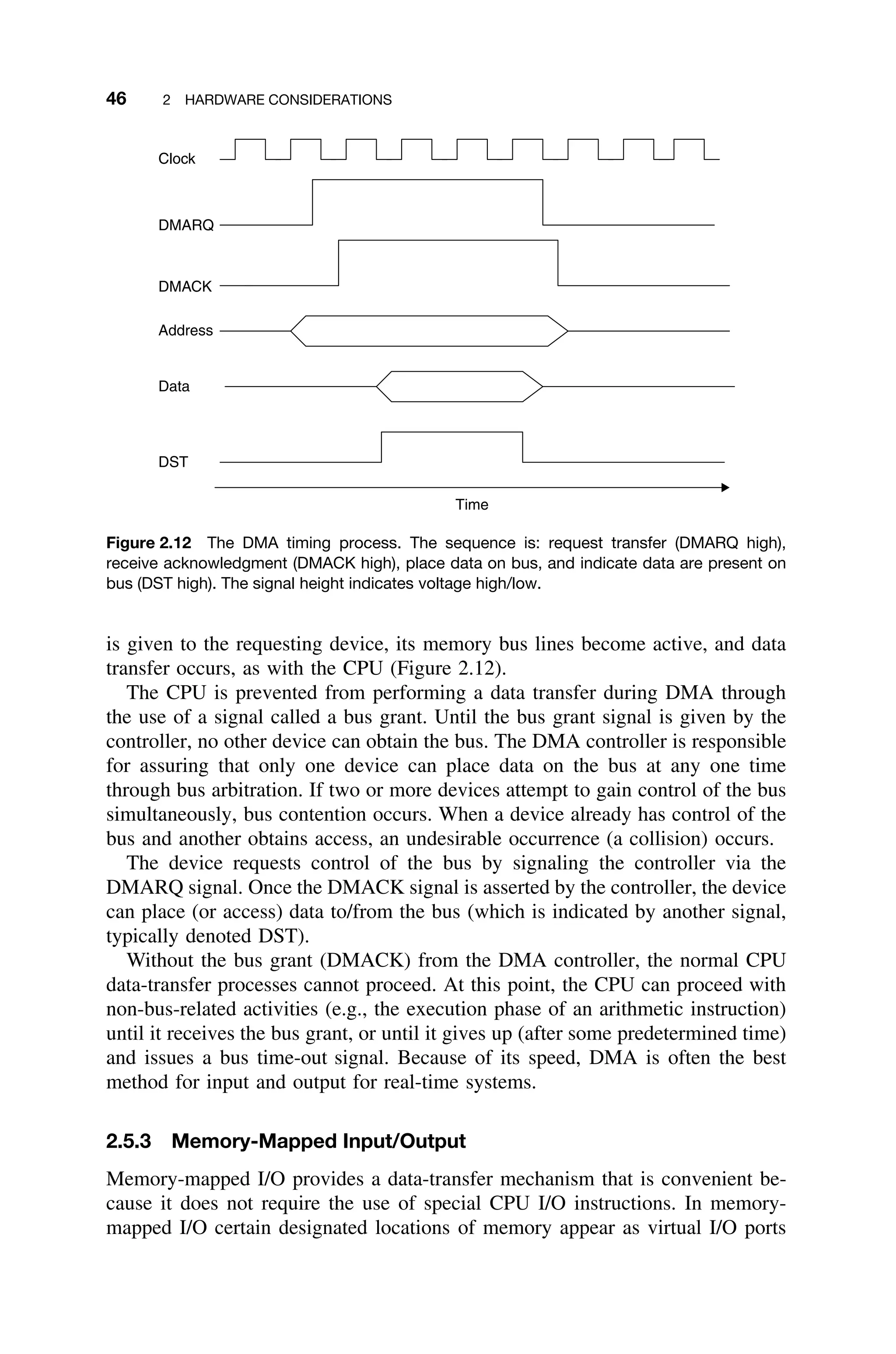
![2
HARDWARE
CONSIDERATIONS
Understanding the underlying hardware of the real-time system allows for efficient
hardware and software resource utilization. Although it is desirable for the pro-
gramming language to abstract away hardware details from the designers, this
is usually impossible to achieve – if not at the design state, certainly at the
hardware/software integration stages. Therefore, an understanding of computer
architecture is essential to the real-time systems engineer. While it is not the
intent here to provide a complete review of computer architecture, a brief sur-
vey of the most important issues is appropriate. For a more thorough treatment,
see, for example, [Gilreath03]. Some of the following discussion is adapted from
that resource.
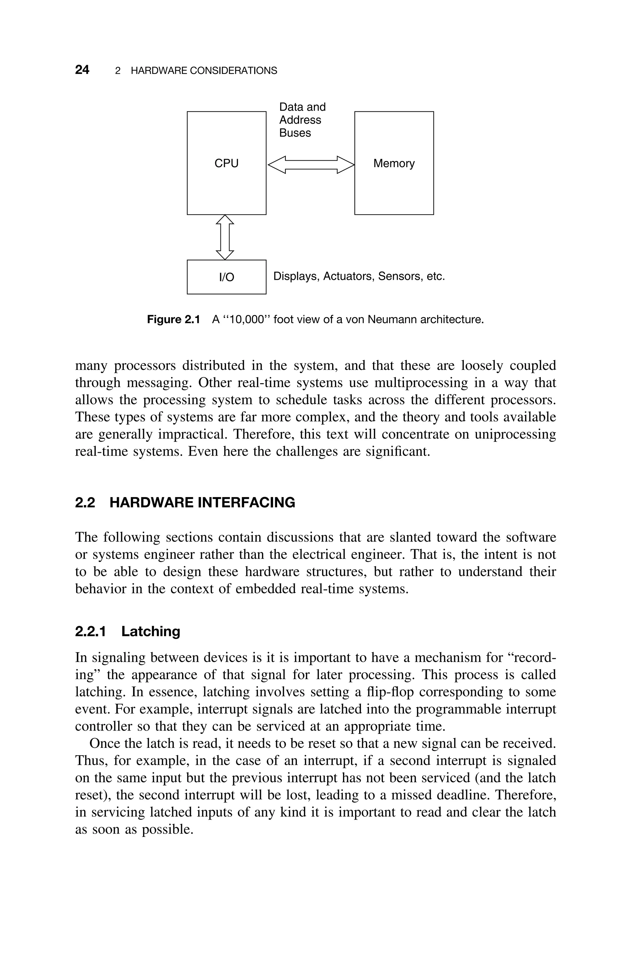
2.1 BASIC ARCHITECTURE
In its simplest form, a computer system consists of a CPU and memory inter-
connected by a bus (Figure 2.1).
There are three systemwide buses: power, address, and data. The power bus
refers to the distribution of power to the various components of the computer sys-
tem; the address bus is the medium for exchanging individual memory addresses,
and therein the data bus is used to move data between the various components
in the system. When referring to the system bus, the address and data buses
collectively are generally what are meant.
For the most part, this book deals with single-processor (uniprocessing) sys-
tems. Some real-time systems are multiprocessing in the sense that there are
Real-Time Systems Design and Analysis, By Phillip A. Laplante
ISBN 0-471-22855-9 2004 Institute of Electrical and Electronics Engineers
23](https://image.slidesharecdn.com/epdf-230618090952-bdcb6616/75/epdf-pub_real-time-systems-design-and-analysis-pdf-46-2048.jpg)
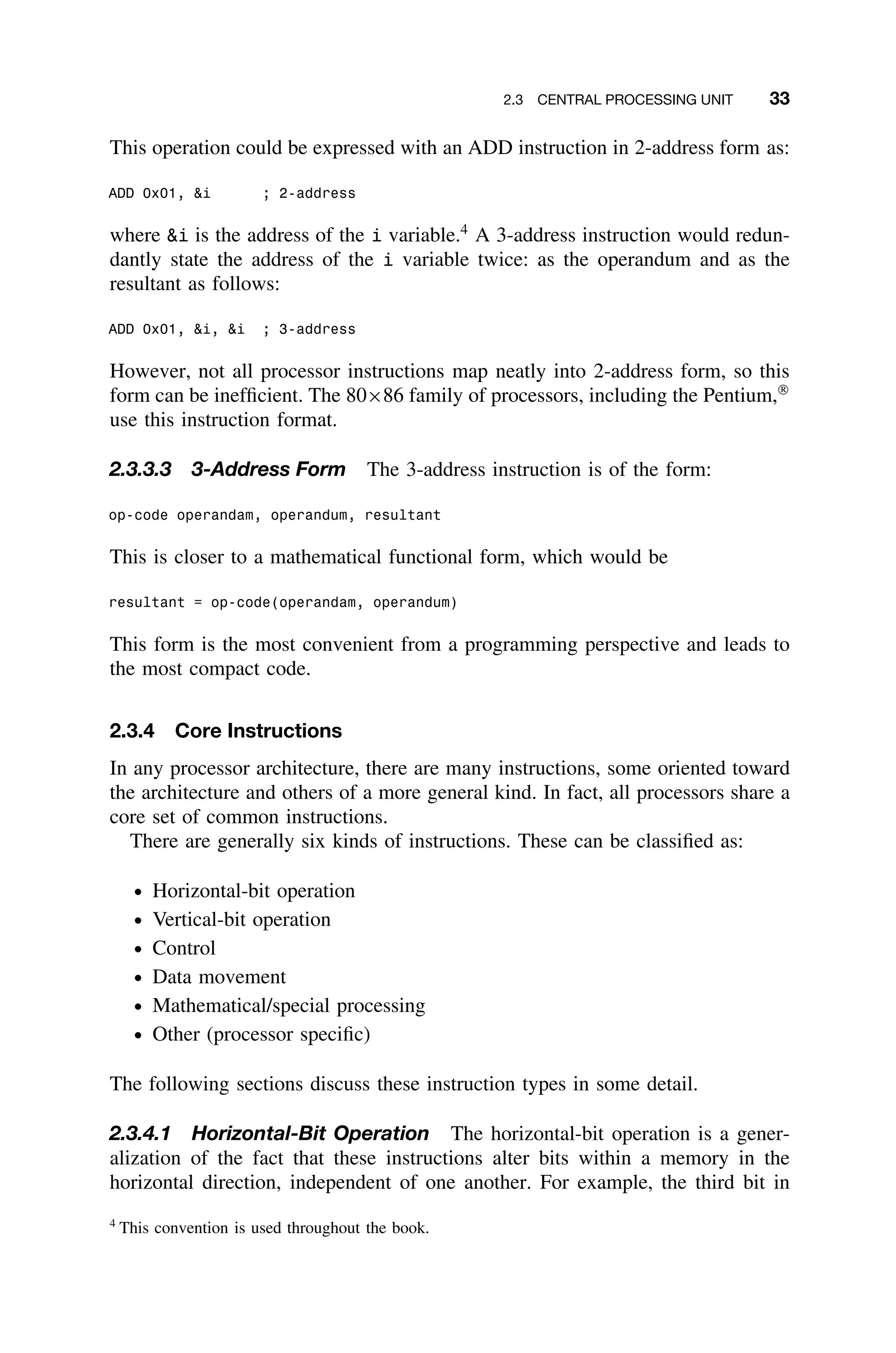
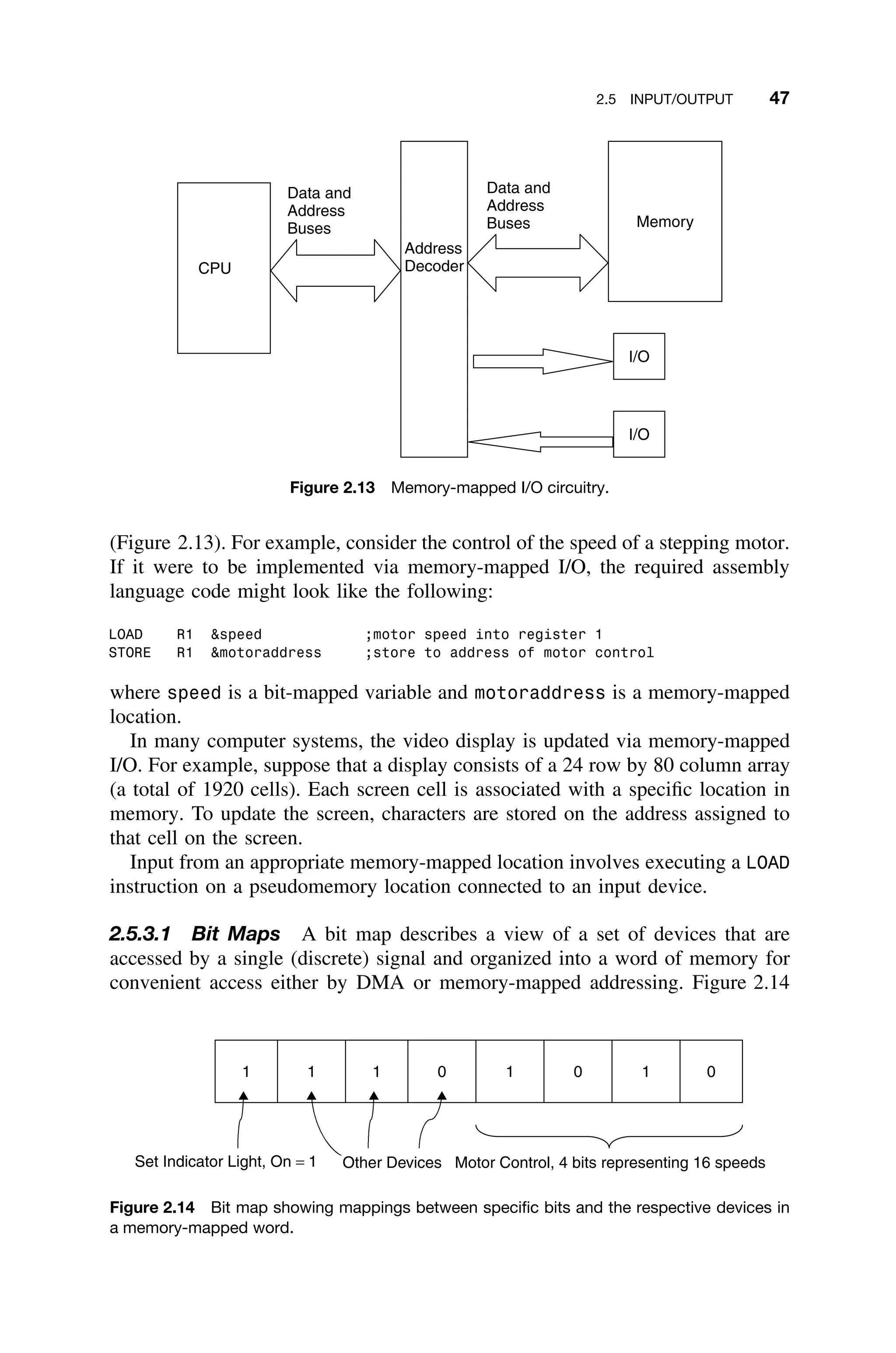
![2.3 CENTRAL PROCESSING UNIT 29
can support the multiple speeds on a single bus, and is flexible – the standard
supports freeform daisy chaining and branching for peer-to-peer implementations.
It is also hot pluggable, that is, devices can be added and removed while the bus
is active.
FireWire supports two types of data transfer: asynchronous and isochronous.
For traditional computer memory-mapped, load, and store applications, asyn-
chronous transfer is appropriate and adequate. Isochronous data transfer provides
guaranteed data transport at a predetermined rate. This is especially important for
multimedia applications where uninterrupted transport of time-critical data and
just-in-time delivery reduce the need for costly buffering. This makes it ideal for
devices that need to transfer high levels of data in real time, such as cameras,
VCRs, and televisions.
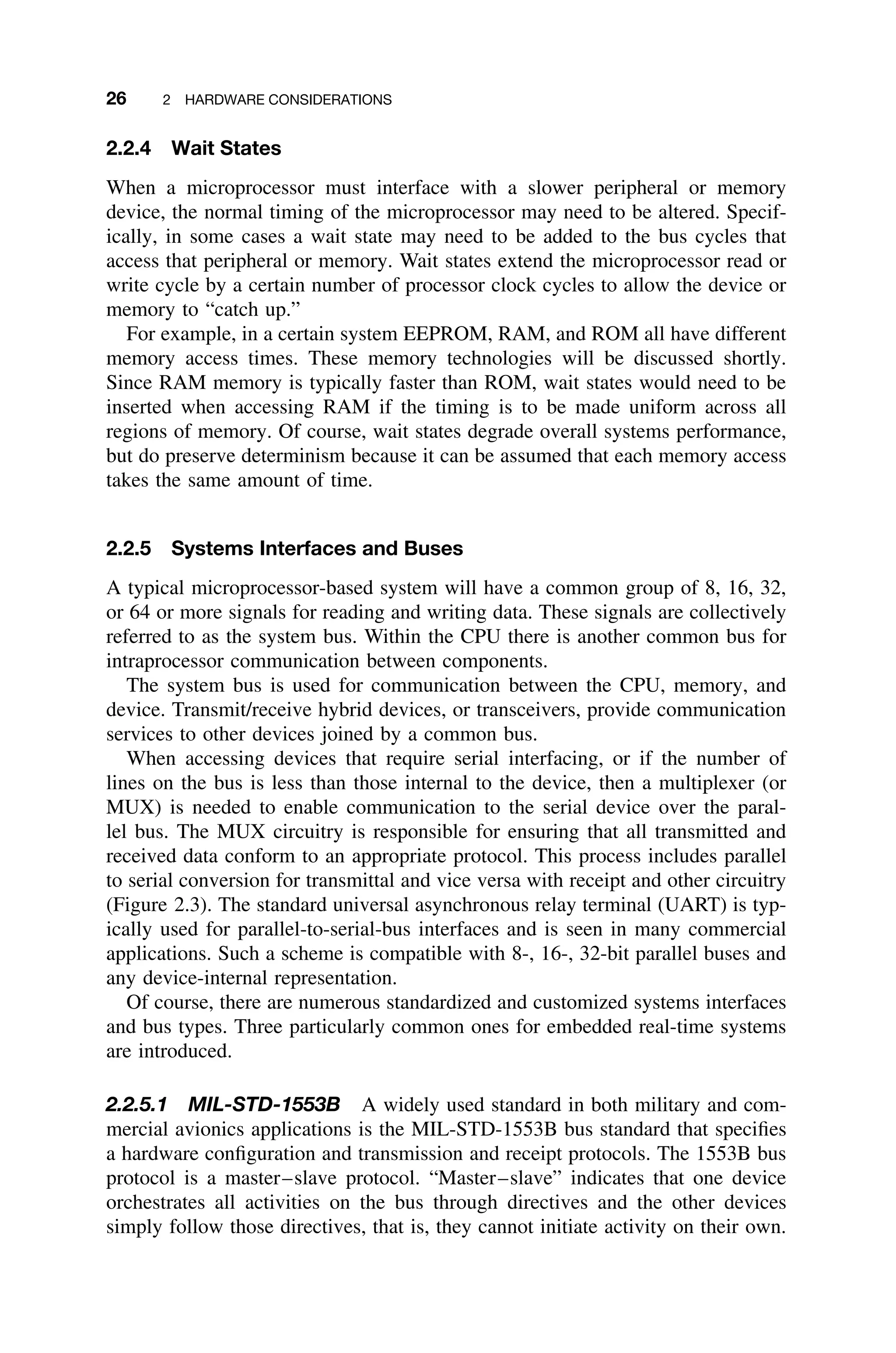
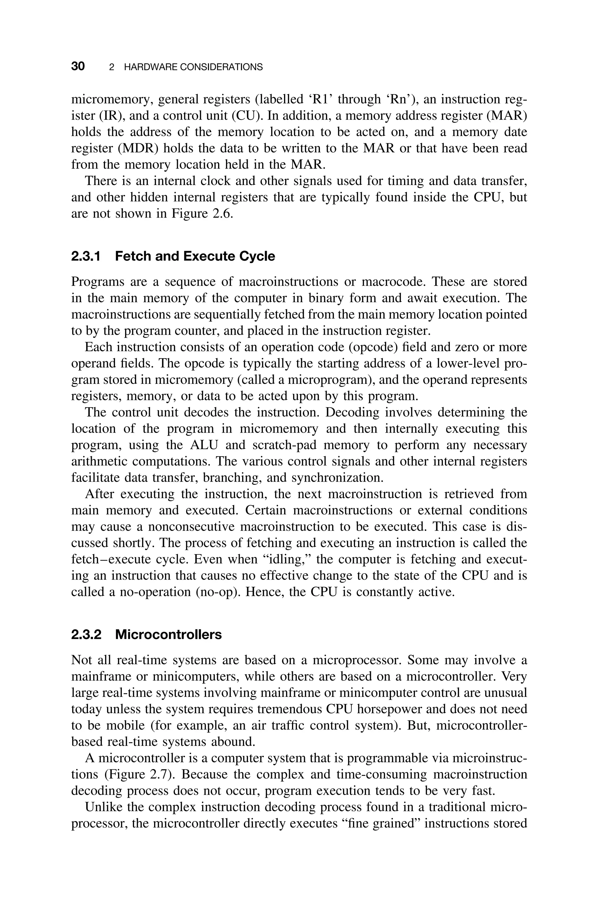
2.3 CENTRAL PROCESSING UNIT
A reasonable understanding of the internal organization of the CPU is quite
helpful in understanding the basic principles of real-time response; hence, those
concepts are briefly reviewed here.1
The CPU can be thought of as containing several components connected by
its own internal bus, which is distinct from the memory and address buses of
the system. As shown in Figure 2.6 the CPU contains a program counter (PC),
an arithmetic logic unit (ALU), internal CPU memory–scratch pad memory and
PC
SR
IR
MDR
R1
MAR
Rn
…
Stack
Pointer
Micro
Memory
Control
Unit
Interrupt
Controller
CPU
Address Bus
Data Bus
Collectively known
as the “bus” or
“system bus”
Figure 2.6 Partial, stylized, internal structure of a typical CPU. The internal paths represent
connections to the internal bus structure. The connection to the system bus is shown on
the right.
1
Some of the following discussion in this section is adapted from Computer Architecture: A Mini-
malist Perspective by Gilreath and Laplante [Gilreath03].](https://image.slidesharecdn.com/epdf-230618090952-bdcb6616/75/epdf-pub_real-time-systems-design-and-analysis-pdf-52-2048.jpg)

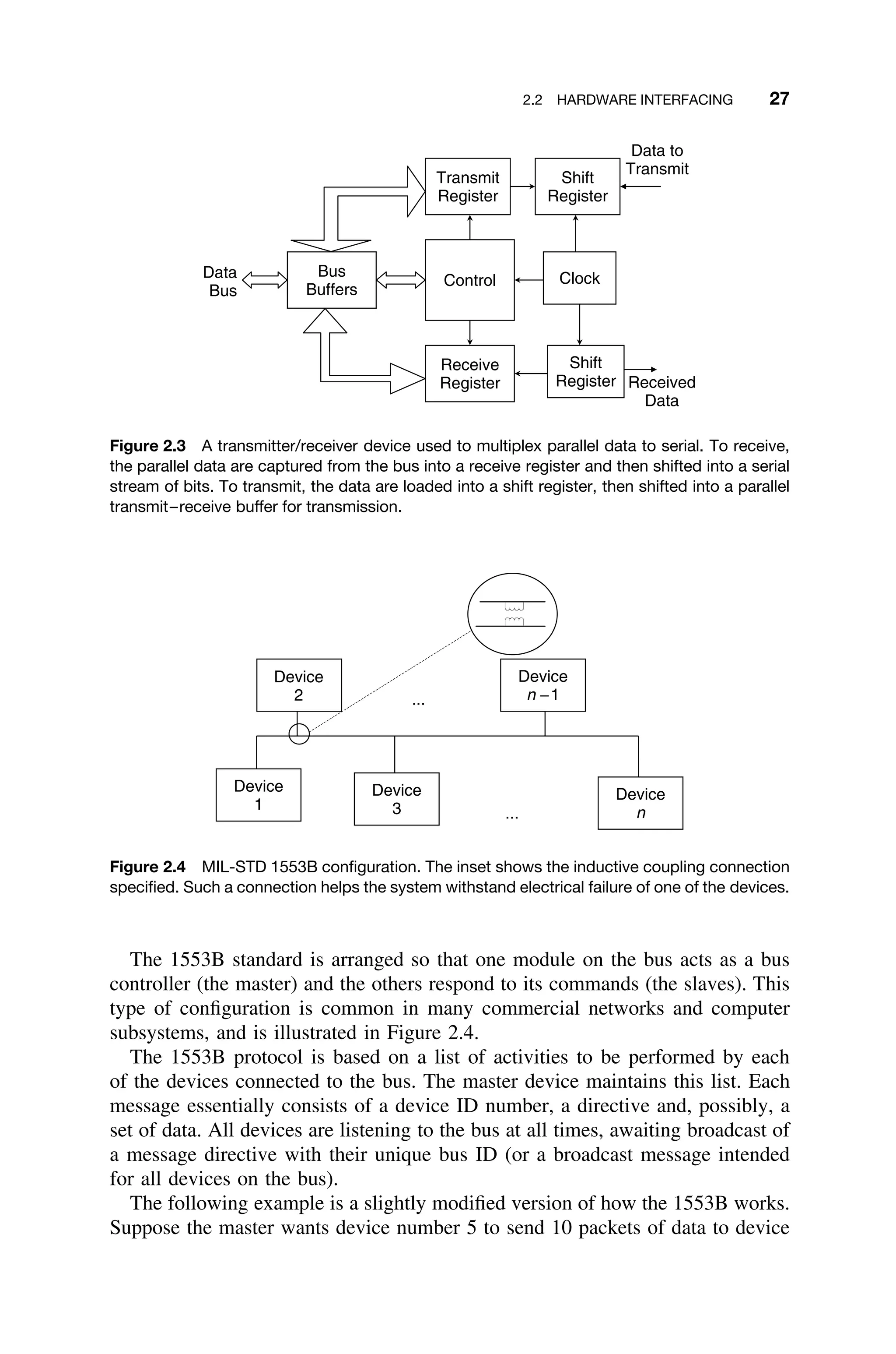
![2.6 ENHANCING PERFORMANCE 57
F D X W
F D X W
F D X W
F D X W
F D X W
F D X W
F D X W
F D X W
F D X W
F D X W
F D X W
F D X W
F D X
F D
F
Clock Cycles
Figure 2.23 Sequential instruction execution versus pipelined instruction execution. Nine
complete instructions can be completed in the pipelined approach in the same time it takes to
complete three instructions in the sequential (scalar) approach [Gilreath03].
in only six clock cycles, and most of the remaining instructions are completed
within the twelve clock cycles.
Pipelining is a form of speculative execution in that the instructions that are
prefetched are taken to be the next sequential instructions. If any of the instruc-
tions in the pipeline are a branch instruction, the prefetched instructions further
in the pipeline are no longer valid.
Higher-level pipelines, or superpipelining, can be achieved if the fetch-and-
execute cycle can be decomposed further. For example, a six-stage pipeline can
be achieved, consisting of a fetch stage, two decode stages (needed to support
indirect addressing modes), an execute stage, a write-back stage (which finds
completed operations in the buffer and frees corresponding functional units), and
a commit stage (in which the validated results are written back to memory).
Another approach to pipelining is to use redundant hardware to replicate one
or more stages in the pipeline. Such a design is called a superscalar architecture.
Furthermore, superscalar and superpipelined architectures can be combined to
obtain a superscalar, superpipelined computer.
When a branch instruction is executed, the pipeline registers and flags must
all be reset, that is, the pipeline is flushed, which takes time. Data and input
dependencies can also slow pipeline flowthrough. Pipelining will improve over-
all performance when locality of reference is high. Otherwise, it may degrade
performance.
The real-time systems engineer must realize that before an interrupt can be
handled, the oldest instruction in the pipeline must be completed and then the](https://image.slidesharecdn.com/epdf-230618090952-bdcb6616/75/epdf-pub_real-time-systems-design-and-analysis-pdf-80-2048.jpg)
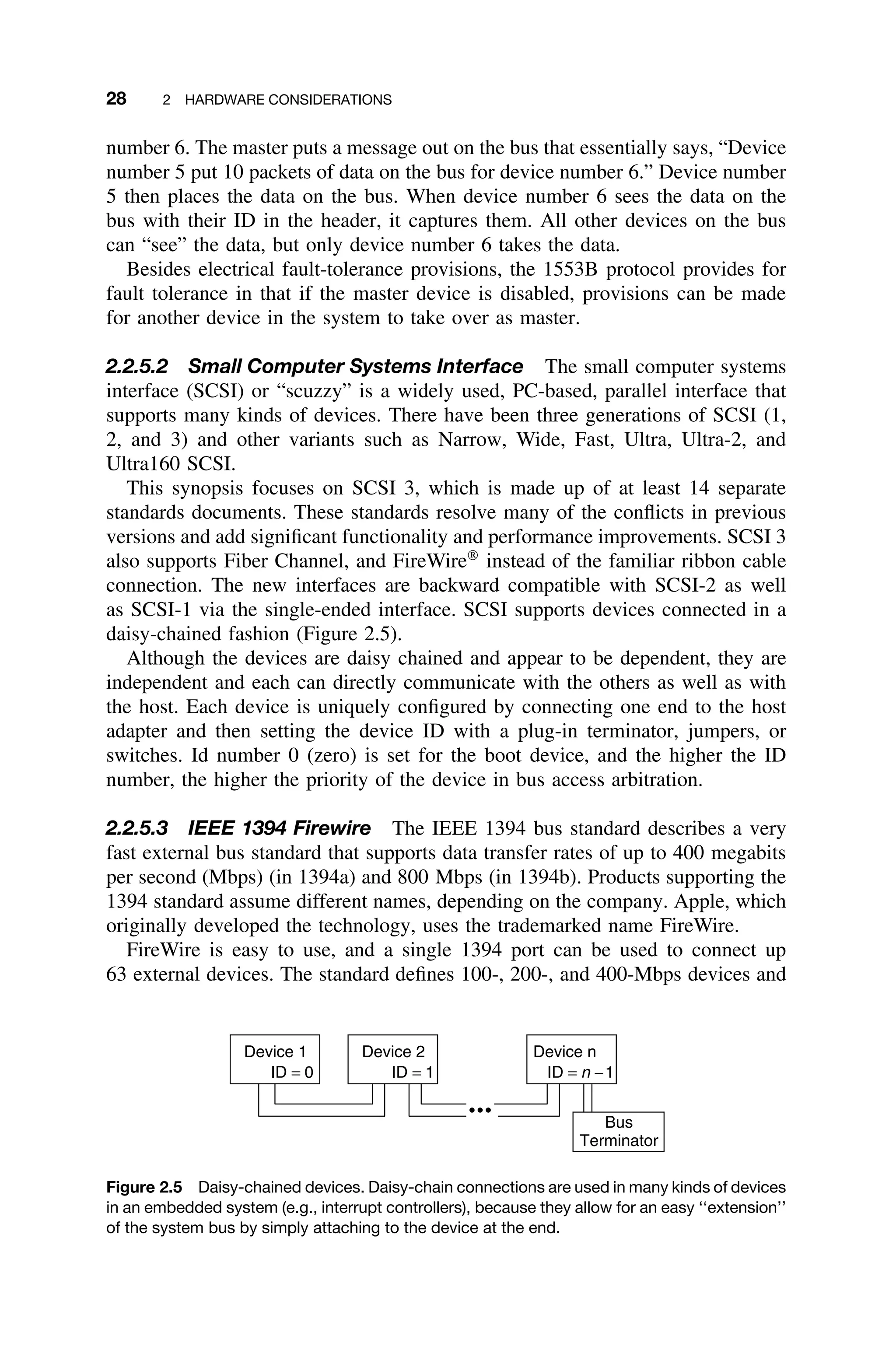
![60 2 HARDWARE CONSIDERATIONS
a b
x1 x2 x3 x4
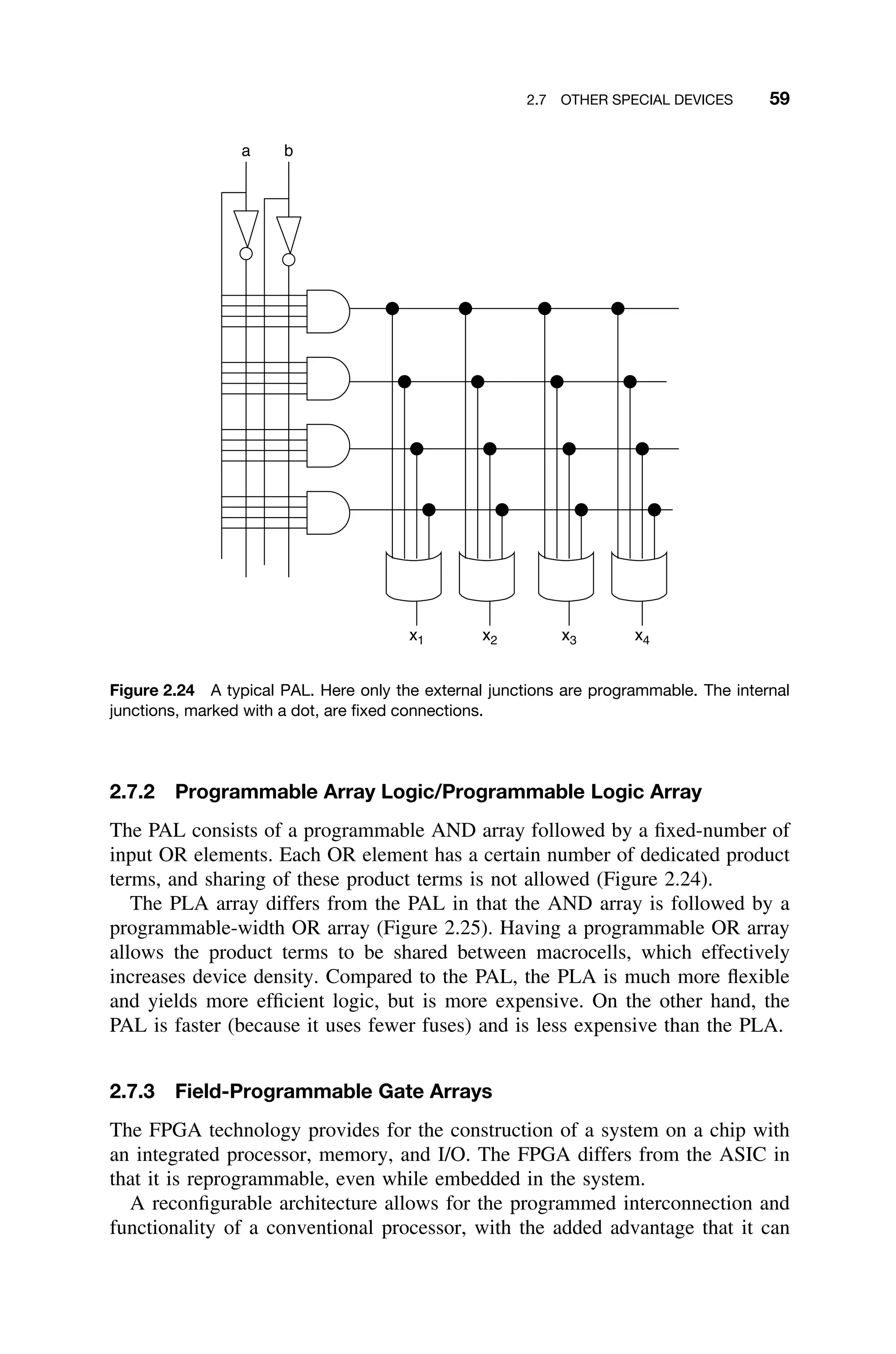
Figure 2.25 A typical PLA. Here all junctions are programmable. That is, they can be selectively
fused to form the necessary product terms.
be tailored to the types of applications involved. Algorithms and functionality
are moved from the software side into the hardware side.
In an FPGA, the programmable logic consists of a series of logic blocks (LBs)
connected in either segmented or continuous interconnect structures (Figure 2.26).
Segmented interconnections are used for short signals between adjacent config-
urable LBs (CLB), while continuous interconnections are used for bus-structured
architectures [Xilinx98].
Each logic block uses one or more look-up tables (LUT) and several bits
of memory. The contents of the LUTs are reprogrammable by changing their
contents. I/O blocks are usually connected to local memories. This design allows
for maximum flexibility, and FPGAs can be used to implement circuit diagrams
into the logic blocks (Figure 2.27). The logic blocks can be configured to exploit
parallelism.
The continuous structure is ideal for connecting large numbers of simple logic
units, such as half adders, full adders, and twos-complement inverters. Moreover,
these logic blocks can also be predesigned to implement higher-level functions,
such as vector addition, convolution, or even an FFT. The ability to reconfigure
logic blocks gives the flexibility of selecting a single instruction and use it to
implement the necessary functionality.](https://image.slidesharecdn.com/epdf-230618090952-bdcb6616/75/epdf-pub_real-time-systems-design-and-analysis-pdf-83-2048.jpg)
![2.7 OTHER SPECIAL DEVICES 61
(a)
Logic
Block
Logic
Block
Logic
Block
Logic
Block
(b)
Logic
Block
Logic
Block
Logic
Block
Logic
Block
Figure 2.26 (a) Segmented and (b) continuous interconnection strategies for FPGA logic
blocks.
I/O I/O I/O I/O I/O I/O I/O
I/O I/O I/O I/O I/O I/O I/O
I/O LB LB LB LB LB I/O
I/O LB LB LB LB LB I/O
I/O LB LB LB LB LB I/O
Figure 2.27 A conceptual illustration of an FPGA showing internal configurable logic blocks
and periphery I/O elements [Gilreath03].
High-level language and sophisticated tool support are available for develop-
ment using FPGAs. Because of standardization, implementations are portable
across commercial FPGA types and further expand the set of available CLBs.
FPGAs have reached usable densities in the hundreds of thousands of gates and
flip-flops that can be integrated to form system-level solutions. Clock structures
can be driven using dedicated clocks that are provided within the system. FPGAs
are infinitely reprogrammable (even within the system) and design modifications
can be made quickly and easily [Xilinx98]. Hence, they are well adapted to many
embedded real-time systems.](https://image.slidesharecdn.com/epdf-230618090952-bdcb6616/75/epdf-pub_real-time-systems-design-and-analysis-pdf-84-2048.jpg)
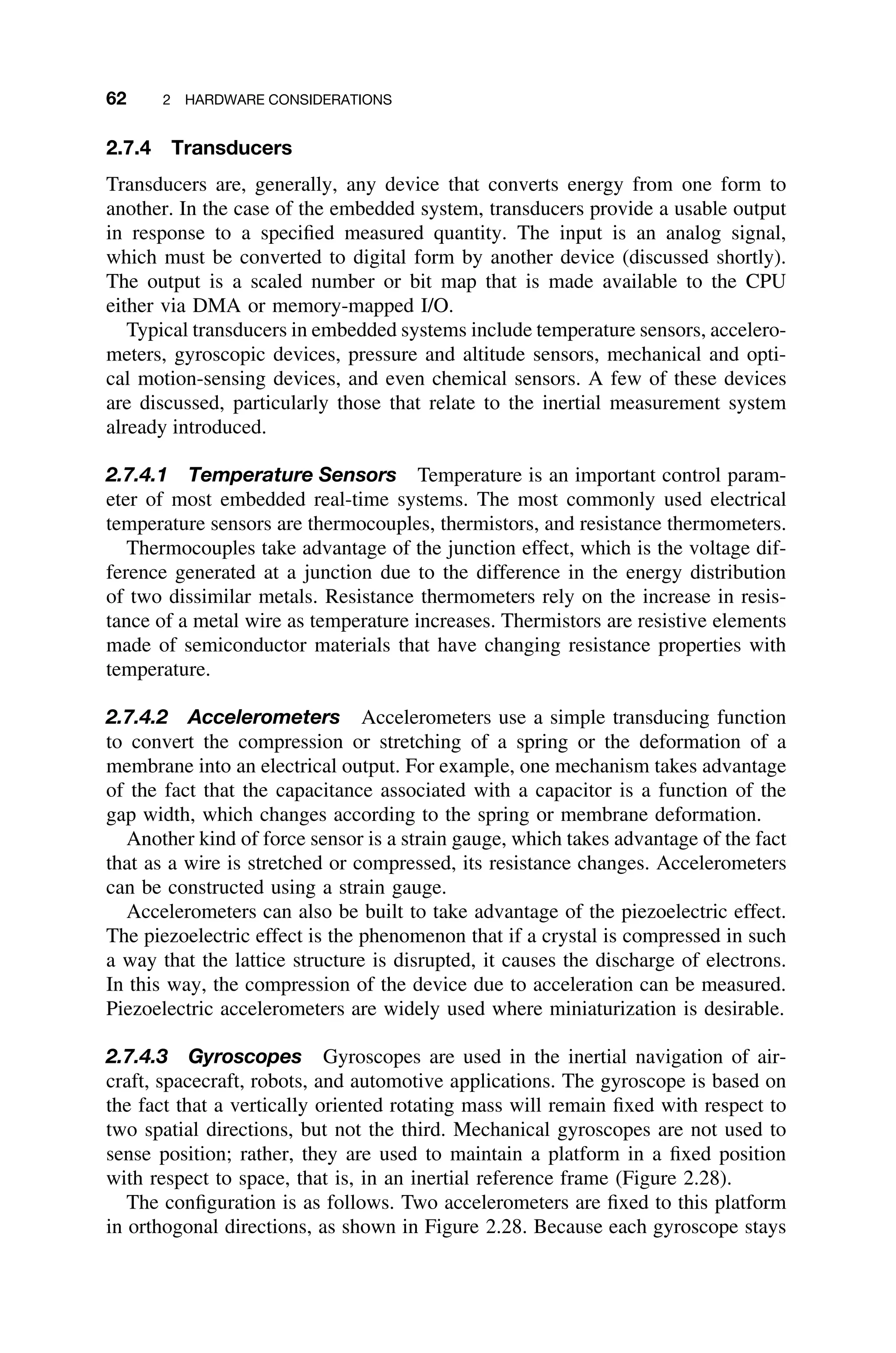
![64 2 HARDWARE CONSIDERATIONS
Ring-laser gyros can also be used for position resolution. These devices are
constructed from two concentric fiber-optic loops. A laser pulse is sent in opposite
directions through each of the two loops. If the vehicle rotates in the direction of
the loops, then one beam will travel faster than the other (twice the angular veloc-
ity of rotation). This difference can be measured and the amount of rotation deter-
mined. One ring-laser gyro each is needed to measure yaw, pitch, and roll angles.
2.7.5 Analog/Digital Converters
Analog-to-digital (A/D) conversion, or A/D circuitry, converts continuous (ana-
log) signals from various transducers and devices into discrete (digital) ones.
Similar circuitry can be used to convert temperature, sound, pressure, and other
inputs from transducers by using a variety of sampling schemes.
The output of A/D circuitry is a discrete version of the time-varying signal
being monitored. This information can be passed on to the real-time computer
system using any of the three data-transfer methods, but in each case the A/D
circuitry makes available an n-bit number that represents a discrete version of
the signal. The discrete version of the continuous value can be treated as a
scaled number.
The key factor in the service of A/D circuitry for time-varying signals is the
sampling rate. In order to convert an analog signal into a digital form without loss
of information, samples of the analog signal must be taken at twice the rate of
the highest-frequency component of the signal (the Nyquist rate). Thus, a signal
with highest-frequency component at 60 hertz must be sampled at 120 times per
second. This implies that software tasks serving A/D circuitry must run at least
at the same rate, or risk losing information. This consideration is an inherent part
of the design process for the scheduling of tasks.
2.7.6 Digital/Analog Converters
Digital-to-analog (D/A) conversion, or D/A circuitry, performs the inverse func-
tion of A/D circuitry; that is, it converts a discrete quantity to a continuous one.
D/A devices are used to allow the computer to output analog voltages based on
the digital version stored internally. Communication with D/A circuitry uses one
of the three input/output methods discussed.
2.8 NON-VON-NEUMANN ARCHITECTURES
The von Neumann bottleneck refers to the fact that only one instruction or one
datum can occupy the bus at any one time. In addition, only one instruction
can be executed at any given time. Architectural enhancements such as caching,
pipelining, and coprocessing have already been discussed as workarounds to
the fundamental von Neumann bottleneck and serial instruction execution
constraints.8
8
Some of the following discussion in this section is adapted from Computer Architecture: A Mini-
malist Perspective by Gilreath and Laplante [Gilreath03]](https://image.slidesharecdn.com/epdf-230618090952-bdcb6616/75/epdf-pub_real-time-systems-design-and-analysis-pdf-87-2048.jpg)
![2.8 NON-VON-NEUMANN ARCHITECTURES 65
Ring Hyper cube Mesh
Figure 2.29 Three different multiprocessor interconnection schemes: (a) ring, (b) mesh, (c) hy-
percube. There are, of course, many other configurations [Gilreath03].
2.8.1 Parallel Systems
The major difference between two parallel systems is the means for which data
are exchanged and interchanged between processors. The two mechanisms for
data interchange are message passing and shared memory.
Message passing involves exchanging discrete messages between processors.
The standard 1553B protocol is one architecture for message passing. Message
passing is a software-oriented approach to parallelism, in that the actual proces-
sors can be distributed across a network.
Another parallel metric is the interconnection among the processors, mea-
sured in terms of number of connections for processors to communicate with one
another. There are many different interconnection schemes. The more common
ones include ring, mesh, or hypercube (Figure 2.29) and the bus interconnection
topology used in 1553B (Figure 2.4).
Shared memory among the processors is a hardware-oriented solution. Shared
memory uses a model where each processor can address another processor as
memory. This is a nonuniform means of interchanging data, as memory for
a processor is different from memory to a shared memory space, which are
the other processor registers. Shared memory is often organized into different
configurations, such as interleaved or distributed memory. The programmable
random-access machine (PRAM) is the general form used for parallel shared-
memory systems.
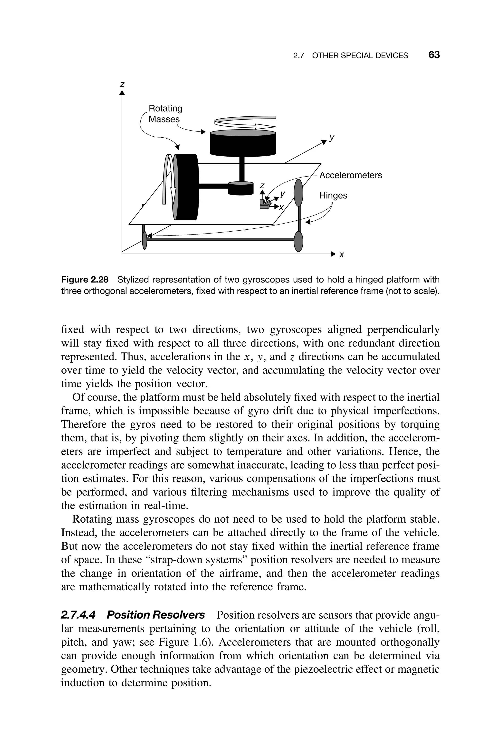
2.8.2 Flynn’s Taxonomy for Parallelism
The generally accepted taxonomy of parallel systems was proposed by Flynn
[Flynn66]. The classification is based on the notion of two streams of information
flow to a processor; instructions, and data. These two streams can be either single
or multiple, given four classes of machines:
1. Single instruction, single data (SISD)
2. Single instruction, multiple data (SIMD)
3. Multiple instruction, single data (MISD)
4. Multiple instruction, multiple data (MIMD)](https://image.slidesharecdn.com/epdf-230618090952-bdcb6616/75/epdf-pub_real-time-systems-design-and-analysis-pdf-88-2048.jpg)
![2.8 NON-VON-NEUMANN ARCHITECTURES 67
2.8.2.3 Single Instruction, Multiple Data Two computer architectures that
are usually classified as SIMD are systolic and wavefront-array parallel comput-
ers. In both systolic and wavefront processors, each processing element executes
the same (and only) instruction, but on different data.
1. Systolic Processors Systolic processors consist of a large number of uni-
form processors connected in an array topology. Each processor usually performs
only one specialized operation and has only enough local memory to perform
its designated operation, and to store the inputs and outputs. The individual pro-
cessors, or processing elements (PE), take inputs from the top and left, perform
a specified operation, and output the results to the right and bottom. One such
processing element is depicted in Figure 2.30. The processors are connected to
the four nearest neighboring processors in the nearest-neighbor topology.
Processing or firing at each of the cells occurs simultaneously in synchroniza-
tion with a central clock. The name comes from the fact that each cell fires on
this heartbeat. Inputs to the system are from memory stores or input devices at
the boundary cells at the left and top. Outputs to memory or output devices are
obtained from boundary cells at the right and bottom.
Systolic processors are fast and can be implemented in VLSI. They are some-
what troublesome, however, in dealing with propagation delays in the connection
buses and in the availability of inputs when the clock ticks.
2. Wavefront Processor Wavefront processors consist of an array of identical
processors, each with its own local memory and connected in a nearest-neighbor
topology. Each processor usually performs only one specialized operation.
Hybrids containing two or more different type cells are possible. The cells fire
asynchronously when all required inputs from the left and top are present. Outputs
c
PE
y
x z = f (x, y)
q =g (x, y)
PE PE PE
PE PE PE PE
PE PE PE PE
Figure 2.30 A systolic computer showing basic processing element (PE) and mesh configu-
ration of multiple elements [Gilreath03].](https://image.slidesharecdn.com/epdf-230618090952-bdcb6616/75/epdf-pub_real-time-systems-design-and-analysis-pdf-90-2048.jpg)
![68 2 HARDWARE CONSIDERATIONS
then appear to the right and below. Unlike the systolic processor, the outputs are
the unaltered inputs. That is, the top input is transmitted unaltered to the bottom
output bus, and the left input is transmitted unaltered to the right output bus.
Also, different from the systolic processor, outputs from the wavefront processor
are read directly from the local memory of selected cells and output obtained
form boundary cells. Inputs are still placed on the top and left input buses of
boundary cells. The fact that inputs propagate through the array unaltered like a
wave gives this architecture its name.
Wavefront processors combine the best of systolic architectures with data flow
architectures. That is, they support an asynchronous data flow computing struc-
ture; timing in the interconnection buses and at input and output devices is not a
problem. Furthermore, the structure can be implemented in VLSI.
2.8.2.4 Multiple Instruction, Multiple Data MIMD computers involve
large numbers of processors that are capable of executing more than one instruc-
tion and on more than one datum at any instant. Except for networks of dis-
tributed multiprocessors working on the same problem (grid computing), these
are “exotic” architectures. Two paradigms that follow MIMD are data flow com-
puters and transputers.
1. Data Flow Architectures Data flow architectures use a large number of
special processors in a topology in which each of the processors is connected
to every other. Each of the processors has its own local memory and a counter.
Special tokens are passed between the processors asynchronously. These tokens,
called activity packets, contain an opcode, operand count, operands, and list of
destination addresses for the result of the computation. An example of a generic
activity packet is given in Figure 2.31.
Each processor’s local memory is used to hold a list of activity packets for that
processor, the operands needed for the current activity packet, and a counter used
Opcode
Argument 1
Argument n
Target 1
Target m
Figure 2.31 Generic activity template for data flow machine [Gilreath03].](https://image.slidesharecdn.com/epdf-230618090952-bdcb6616/75/epdf-pub_real-time-systems-design-and-analysis-pdf-91-2048.jpg)
![2.8 NON-VON-NEUMANN ARCHITECTURES 69
to keep track of the number of operands received. When the number of operands
stored in local memory is equivalent to that required for the operation in the
current activity packet, the operation is performed and the results are sent to the
specified destinations. Once an activity packet has been executed, the processor
begins working on the next activity packet in its execution list.
Data flow architectures are an excellent parallel solution for signal processing,
but require a cumbersome graphical programming language, and hence are rarely
seen today.
2. Transputers Transputers are fully self-sufficient, multiple instruction set,
von Neumann processors. The instruction set includes directives to send data or
receive data via ports that are connected to other transputers. The transputers,
though capable of acting as a uniprocessor, are best utilized when connected in a
nearest-neighbor configuration. In a sense, the transputer provides a wavefront or
systolic processing capability, but without the restriction of a single instruction.
Indeed, by providing each transputer in a network with an appropriate stream of
data and synchronization signals, wavefront, or systolic computers – which can
change configurations – can be implemented.
Transputers have been used in some embedded real-time applications, and
commercial implementations are available. Moreover, tool support, such as the
multitasking language occam-2, has made it easier to build transputer-based appli-
cations. Nevertheless, transputer-based systems are relatively rare, especially in
the United States.
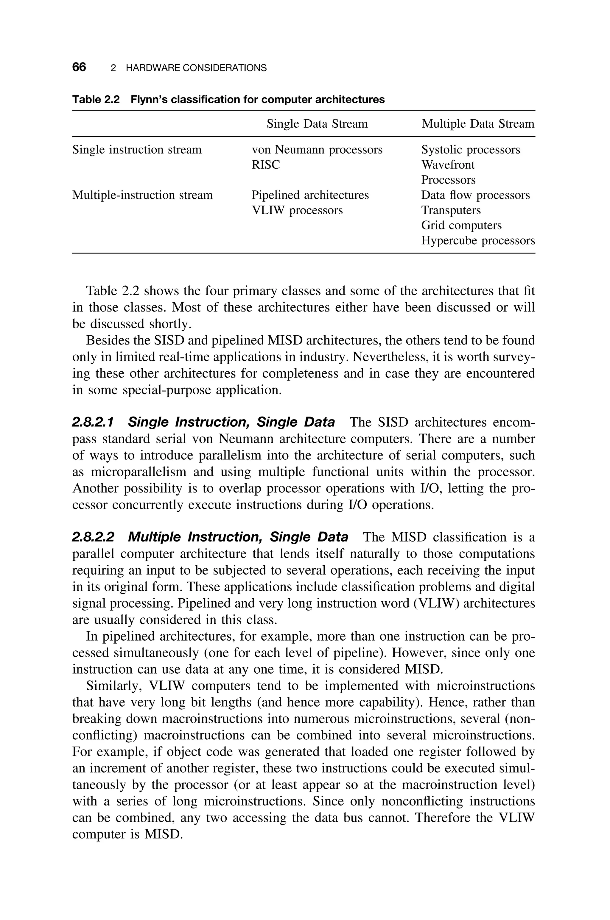
3. Transport Triggered Architecture A special case of the MIMD computer
is the distributed heterogeneous architecture in which a number of independent
von Neumann CPUs communicate over a network and employ a time-driven pro-
cessing model rather than an event-driven one. One example, the time-triggered
architecture (TTA) developed by Kopetz and others, can be used for imple-
menting distributed hard real-time systems [Kopetz97]. TTA models a distributed
real-time system as a set of nodes interconnected by a real-time communication
system (Figure 2.32).
TTA is based on fault-tolerant clock synchronization. Each node consists of a
communication controller and a host computer, which are provided with a global,
synchronized clock with a 1-microsecond tick duration. Each node is autonomous
but communicates with other nodes over a replicated broadcast channel. Using
time division multiple access (TDMA), each node is allocated a time slot in which
it can send information on the bus to one or more receiving nodes, through a
unique addressing scheme. It is thus possible to predict the latency of all messages
on the bus, which guarantees hard real-time message delivery. Furthermore, since
the messages are sent at a predetermined point in time, the latency jitter is
minimal. By comparing the known point in time at which a particular message
was sent and when it is received, host computers can synchronize their clocks
without the overhead of messages [Kopetz98]. Each individual node in the TTA
needs to be designed as a self-sufficient real-time system. But the architecture
provides a very reliable and predictable mechanism for communication between](https://image.slidesharecdn.com/epdf-230618090952-bdcb6616/75/epdf-pub_real-time-systems-design-and-analysis-pdf-92-2048.jpg)
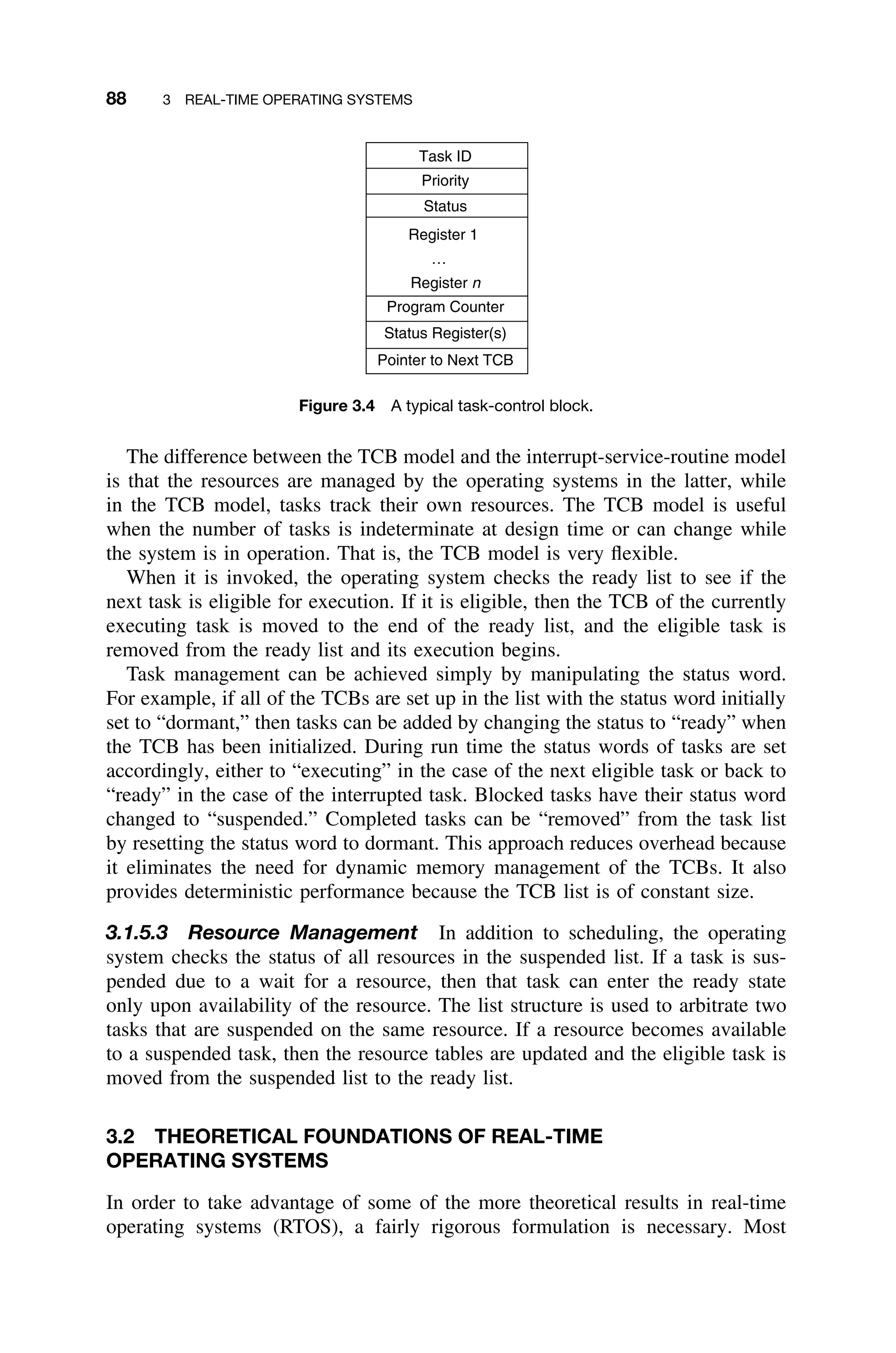
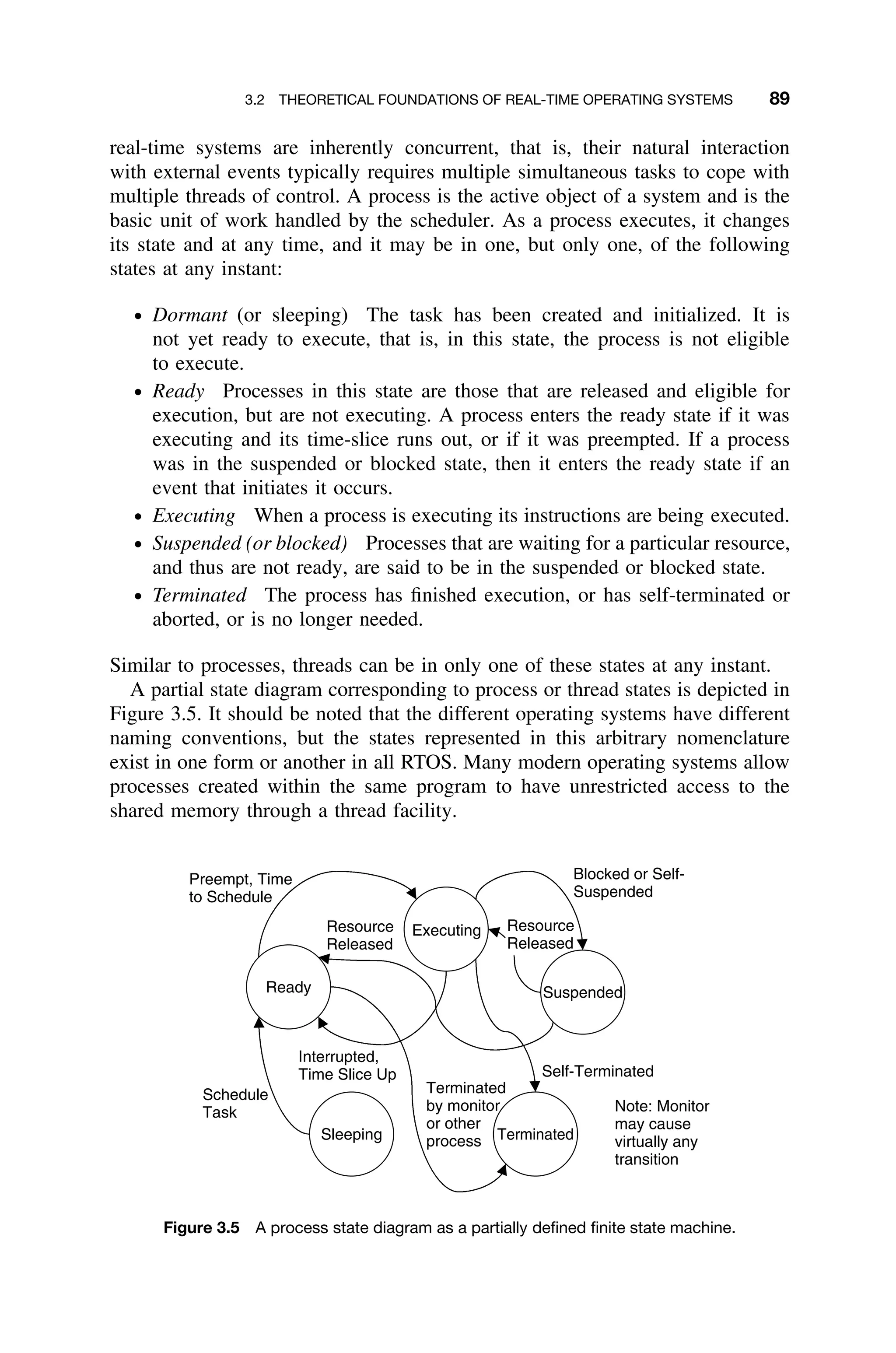
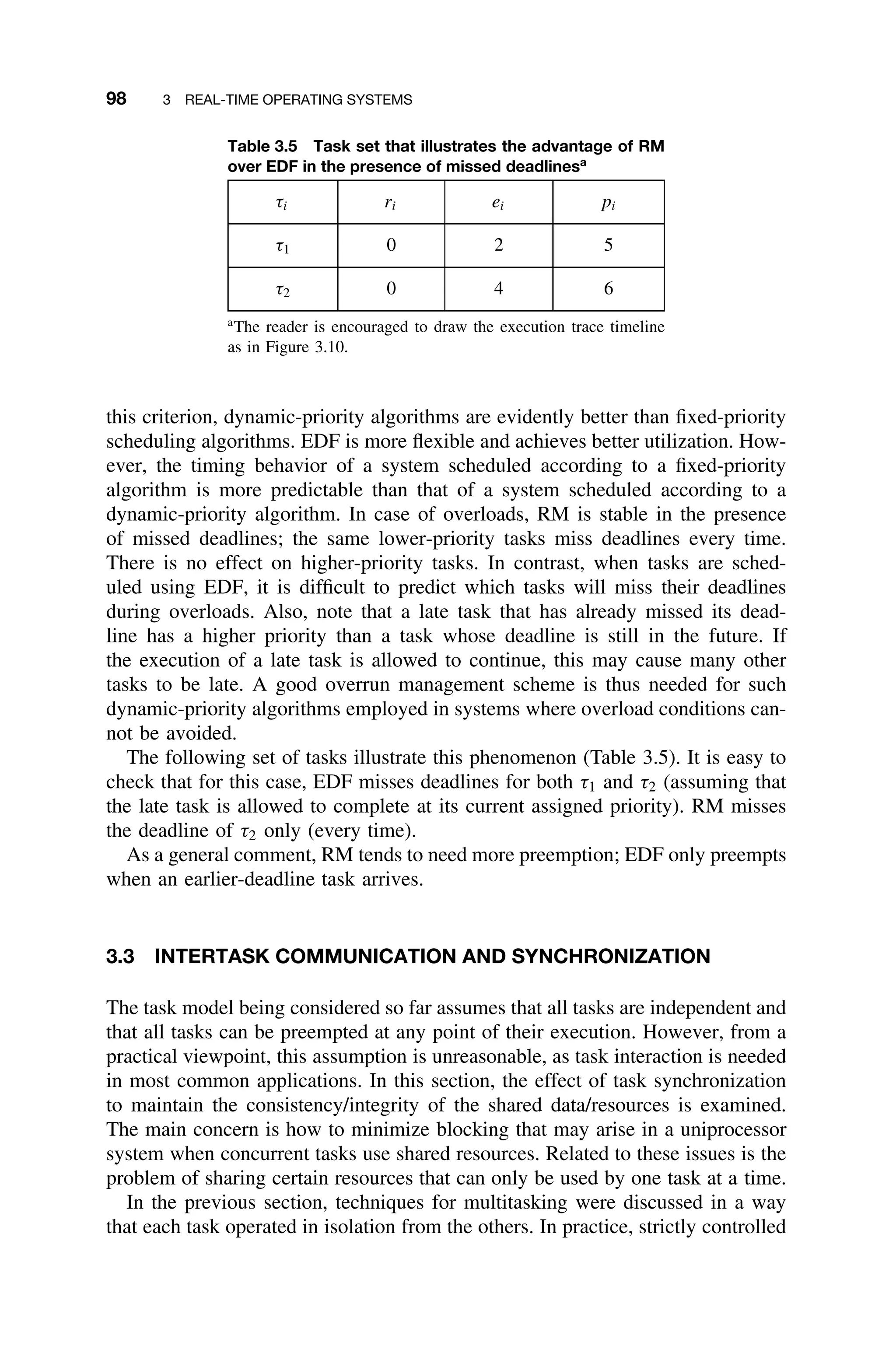
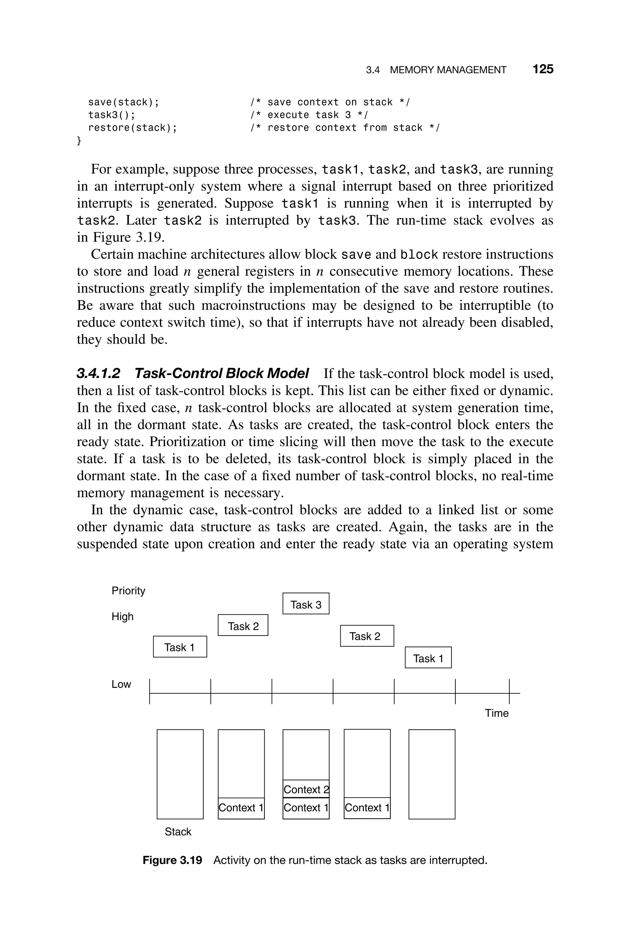
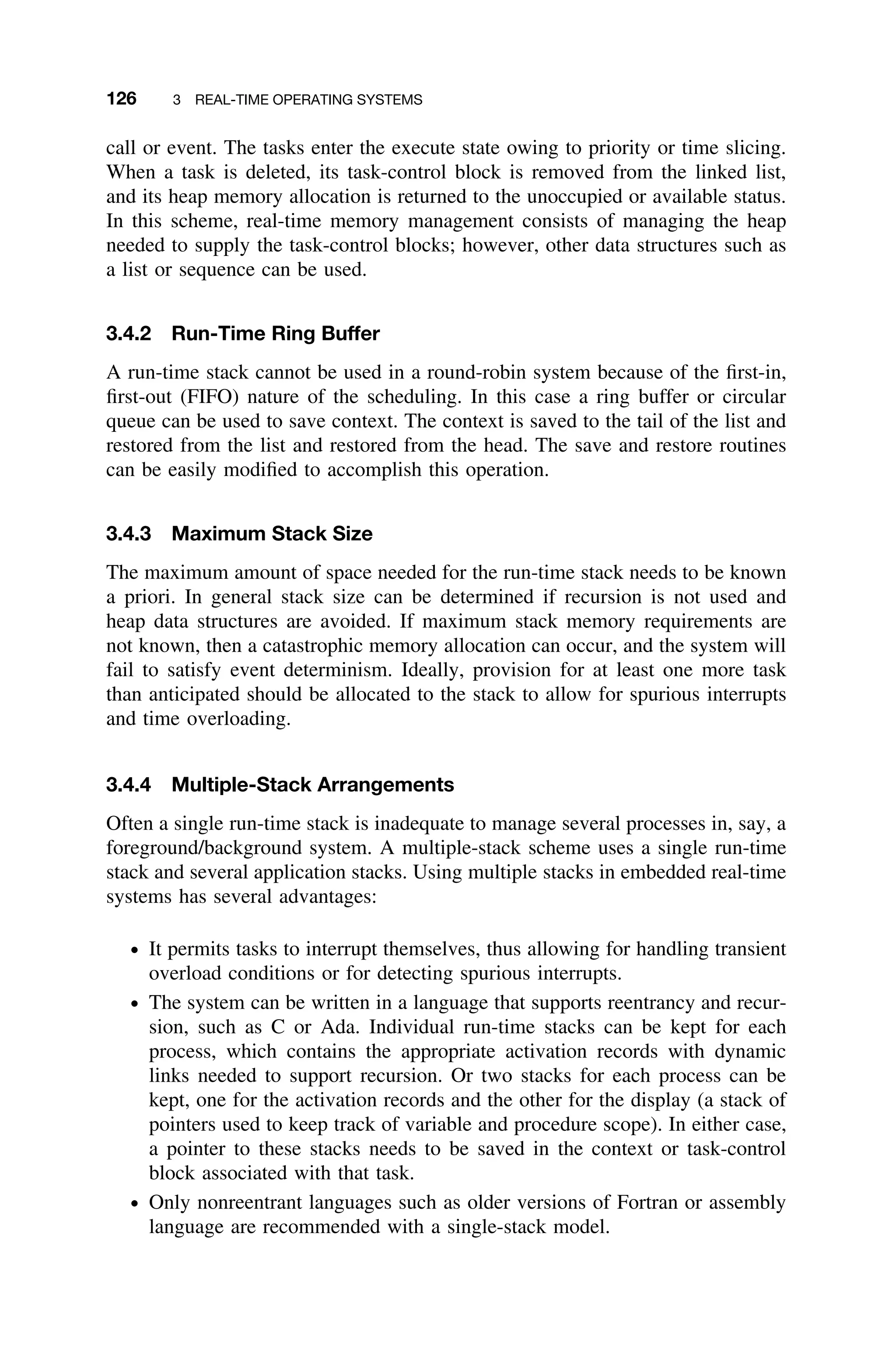
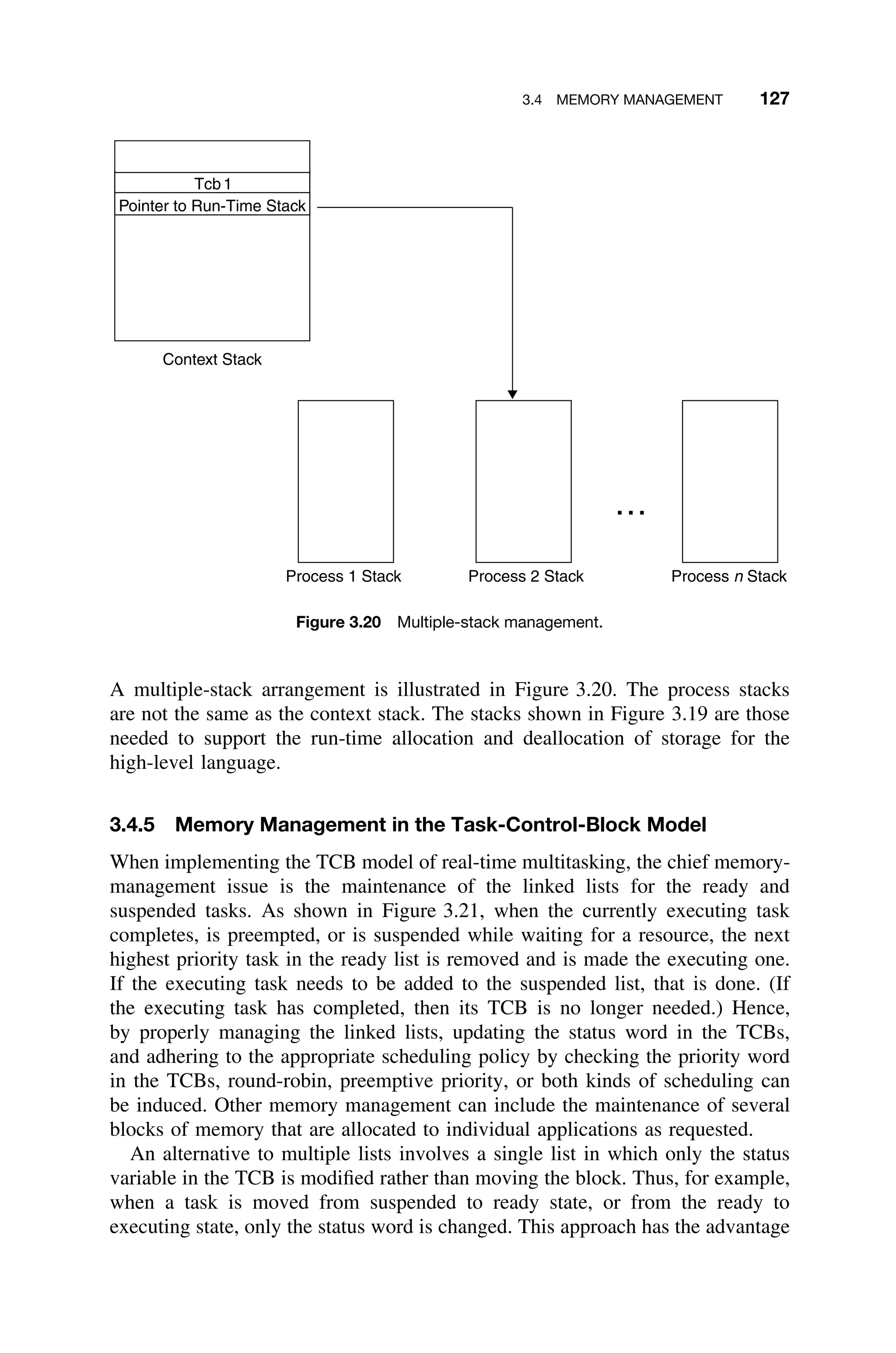
![94 3 REAL-TIME OPERATING SYSTEMS
3.2.4 Fixed-Priority Scheduling–Rate-Monotonic Approach
In the fixed-priority scheduling policy, the priority of each periodic task is fixed
relative to other tasks. A seminal fixed-priority algorithm is the rate-monotonic
(RM) algorithm [Liu73]. It is an optimal static priority algorithm for the task
model previously described, in which a task with a shorter period is given a
higher priority than a task with a longer period. The theorem, known as the rate-
monotonic theorem is the most important (and useful) result of real-time systems
theory. It can be stated as follows.
Theorem (Rate-monotonic) [Liu73] Given a set of periodic tasks and preemptive pri-
ority scheduling, then assigning priorities such that the tasks with shorter periods have
higher priorities (rate-monotonic), yields an optimal scheduling algorithm.
In other words, optimality of RM implies that if a schedule that meets all the
deadlines exists with fixed priorities, then RM will produce a feasible schedule. A
critical instant of a task is defined to be an instant at which a request for that task
will have the largest response time. Liu and Layland proved that a critical instant
for any task occurs whenever the task is requested simultaneously with requests
for all higher-priority tasks. It is then shown that to check for RM schedulability
it suffices to check the case where all tasks phasings are zero [Liu73].
The formal proof of the theorem is rather involved. However, a nice sketch of
the proof due to Shaw uses an inductive argument [Shaw01].
Basis Step Consider two fixed but non-RM priority tasks τ1 = (e1, p1, d1) and τ2 =
(e2, p2, d2) where τ2 has the highest priority, and p1 p2. Suppose both processes are
released at the same time. It is clear that this leads to the worst-case response time for τ1.
However, at this point, in order for both processes to be schedulable, it is necessary that
e1 + e2 ≤ pi; otherwise, τ1 could not meet its period or deadlines. Because of this relation
between the compute times and the period (deadline) of τ2, we can obtain a feasible
schedule by reversing priorities, thereby scheduling τ1 first, that is with RM assignment.
Induction Step Suppose that τ1, . . . , τn are schedulable according to RM, with priorities
in ascending order, but the assignment is not RM. Let τi and τi+1, 1 ≤ i n, be the
first two tasks with non-RM priorities. That is, pi pi+1. The “proof” proceeds by
interchanging the priorities of these two processes and showing the set is still schedulable
using the n = 2 result. The proof continues by interchanging non-RM pairs in this fashion
until the assignment is RM. Therefore if a fixed-priority assignment can produce a feasible
schedule, so can RM assignment.
To illustrate rate-monotonic scheduling, consider the task set shown in
Table 3.2.
Figure 3.8 illustrates the RM-schedule for the task set. All tasks are released
at time 0. Since task τ1 has the smallest period, it is the highest priority task and
is scheduled first. Note that at time 4 the second instance of task τ1 is released
and it preempts the currently running task τ3, which has the lowest priority.](https://image.slidesharecdn.com/epdf-230618090952-bdcb6616/75/epdf-pub_real-time-systems-design-and-analysis-pdf-117-2048.jpg)
![3.2 THEORETICAL FOUNDATIONS OF REAL-TIME OPERATING SYSTEMS 95
Table 3.2 Sample task set for utilization calculation
τi ei pi ui = ei/pi
τ1 1 4 0.25
τ2 2 5 0.4
τ3 5 20 0.25
0 4 8 12 16 20
t1 t2 t3
Figure 3.8 Rate-monotonic task schedule.
Here utilization, ui, is equal to the fraction of time a task with period pi and
execution time ei keeps a processor busy. Recall that the processor utilization of
n tasks is given by Equation 1.2, that is U =
n
i=1 ei/pi.
3.2.4.1 Basic Results of Rate-Monotonic Algorithm Policy From a
practical point of view, it is important to know under what conditions a fea-
sible schedule exists in the static-priority case. The following theorem [Liu73]
yields a schedulable utilization of the rate-monotonic algorithm (RMA). Note
that the relative deadline of every task is equal to its period.
Theorem (RMA Bound) Any set of n periodic tasks is RM schedulable if the processor
utilization, U, is no greater than n(21/n
− 1).
This means that whenever U is at or below the given utilization bound, a
schedule can be constructed with RM. In the limit when the number of tasks
n = ∞, the maximum utilization limit is
lim
n→∞
n(21/n
− 1) = ln 2 ≈ 0.69 (3.7)
The calculation of the limit in Equation 3.7 is straightforward but worth docu-
menting. First recall that
d
dx
ax
= (ln a)ax
dx
Hence,
d
dx
2n−1
= (ln 2)2n−1
(−n−2
)](https://image.slidesharecdn.com/epdf-230618090952-bdcb6616/75/epdf-pub_real-time-systems-design-and-analysis-pdf-118-2048.jpg)
![3.2 THEORETICAL FOUNDATIONS OF REAL-TIME OPERATING SYSTEMS 97
completed. One of the most well-known dynamic algorithms, earliest-deadline-
first (EDF), deals with deadlines rather than execution times. The ready task with
the earliest deadline has the highest priority at any point of time.
The following theorem gives the condition under which a feasible schedule
exists under the EDF priority scheme [Liu73].
Theorem [EDF Bound] A set of n periodic tasks, each of whose relative dead-
line equals its period, can be feasibly scheduled by EDF if and only if
n
i=1
(ei/pi) ≤ 1 (3.8)
Figure 3.10 illustrates the EDF scheduling policy. The schedule is produced
for the task set shown in Table 3.4.
Although τ1 and τ2 release simultaneously, τ1 executes first because its deadline
is earliest. At t = 2, τ2 can execute. Even though τ1 releases again at t = 5, its
deadline is not earlier than τ3. This sequence continues until time t = 15 when τ2
is preempted, as its deadline is later (t = 21) than τ1(t = 20); τ2 resumes when
τ1 completes.
3.2.5.1 Basic Results of EDF Policy EDF is optimal for a uniprocessor,
with task preemption being allowed. In other words, if a feasible schedule exists,
then the EDF policy will also produce a feasible schedule. There is never a
processor idling prior to a missed deadline.
3.2.5.2 Comparison of RMA and EDF Policies Schedulable utilization
is a measure of performance of algorithms used to schedule periodic tasks. It
is desired that a scheduling algorithm yield a highly schedulable utilization. By
t2 Preempted
t1 t2
t2 Resumes
0 2 4 6 8 10 12 14 16 18 20 22 24 26 28 30 32 34 36
Figure 3.10 EDF task schedule for task set in Table 3.4.
Table 3.4 Task set for example of EDF scheduling
τi ei pi
τ1 2 5
τ2 4 7](https://image.slidesharecdn.com/epdf-230618090952-bdcb6616/75/epdf-pub_real-time-systems-design-and-analysis-pdf-120-2048.jpg)
![102 3 REAL-TIME OPERATING SYSTEMS
of type ring_buffer that includes an integer array of size of N called con-
tents, namely,
typedef struct ring_buffer
{
int contents[N];
int head;
int tail;
}
It is further assumed that the head and tail indices have been initialized to 0,
that is, the start of the buffer.
An implementation of the read(data,S) and write(data,S) operations,
which reads from and writes to ring buffer S, respectively, are given below in C
code.3
void read (int data, ring_buffer *s)
{
if (s-head==s-tail)
data=NULL; /* underflow */
else
{
data=s-contents +head; /* retrieve data from buffer */
s-head=(s-head+1) % N; /* decrement head index */
}
}
void write (int data, ring_buffer *s)
{
if ((s-tail+1) %N==head)
error(); /* overflow, invoke error handler */
else
{
s-contents+tail=data;
tail=(tail+1) % N; /*take care of wrap-around */
}
}
Additional code is needed to test for the overflow condition in the ring buffer,
and the task using the ring buffer needs to test the data for the underflow (NULL)
value. An overflow occurs when an attempt is made to write data to a full queue.
Underflow is the condition when a task attempts to retrieve data from an empty
buffer. Implementation of these exception handlers is left as Exercise 3.31.
Ring buffers can be used in conjunction with a counting or binary semaphore to
control multiple requests for a single resource such as memory blocks, modems,
and printers.
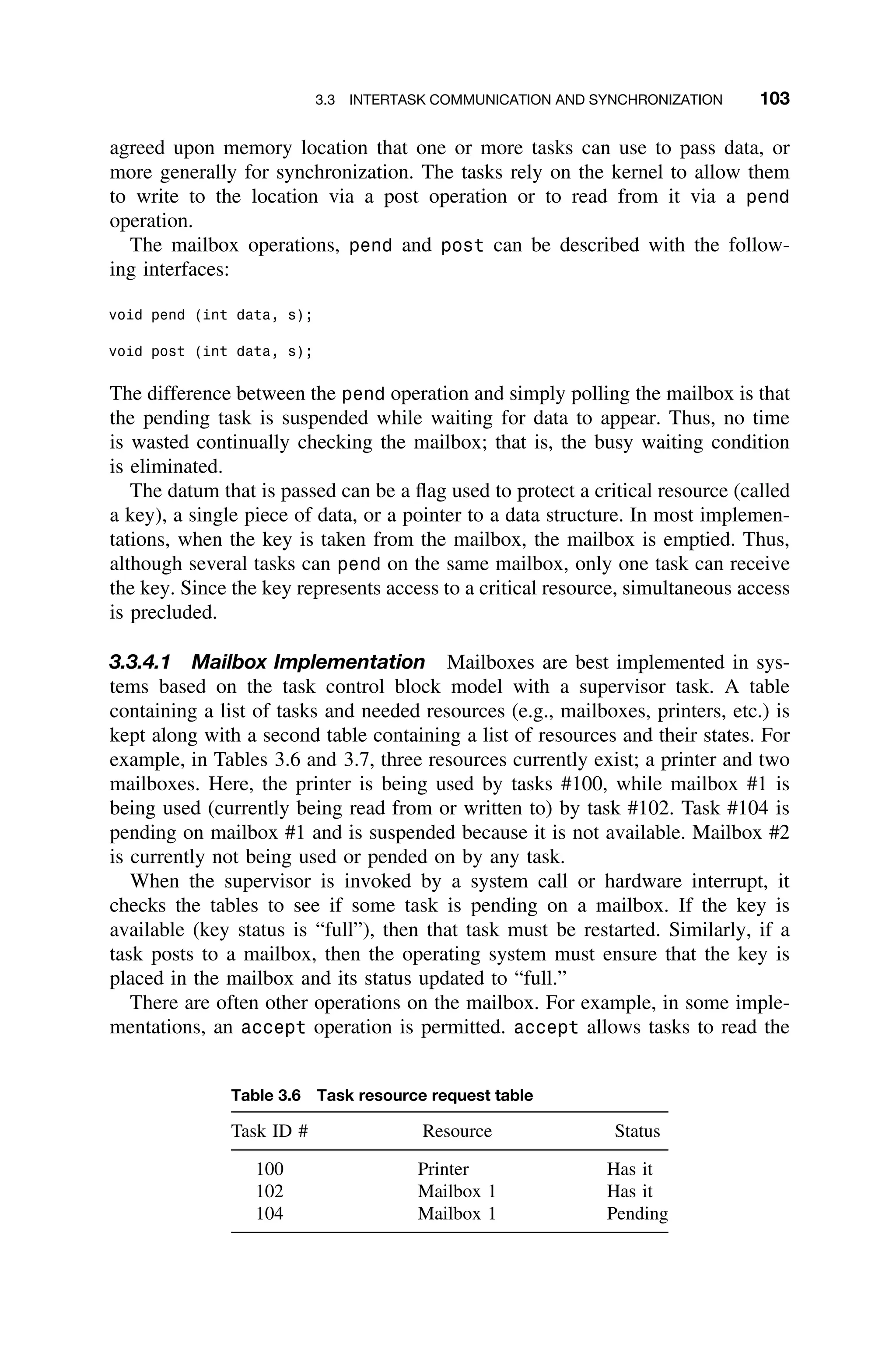
3.3.4 Mailboxes
Mailboxes or message exchanges are an intertask communication device available
in many commercial, full-featured operating systems. A mailbox is a mutually
3
For those unfamiliar with C, the notation “-” indicates accessing a particular field of the structure
that is referenced by the pointer.](https://image.slidesharecdn.com/epdf-230618090952-bdcb6616/75/epdf-pub_real-time-systems-design-and-analysis-pdf-125-2048.jpg)
![3.3 INTERTASK COMMUNICATION AND SYNCHRONIZATION 105
resource results in a collision. The concern, then, is to provide a mechanism for
preventing collisions.
3.3.7 Semaphores
The most common method for protecting critical regions involves a special vari-
able called a semaphore. A semaphore S is a memory location that acts as a lock
to protect critical regions. Two operations, wait and signal are used either to
set or to reset the semaphore. Traditionally, one denotes the wait operation as
P(S) and the signal operations V(S).4
The primitive operations are defined by
the following C code:
void P(int S)
{
while (S == TRUE);
S=TRUE;
}
void V(int S)
{
S=FALSE;
}
The wait operation suspends any program calling until the semaphore S is
FALSE, whereas the signal operation sets the semaphore S to FALSE. Code that
enters a critical region is bracketed by calls to wait and signal. This prevents
more than one process from entering the critical region. Incidentally, recall that C
passes by value unless forced to pass by reference by passing a pointer; therefore,
when calling functions the dereferencing operator “” should be used. However,
for convenience of notation, when a parameter is passed, it is as if the address
of the parameter is passed to the function. Alternatively, the parameter can be
viewed as a global variable.
Now consider two concurrent processes in a multitasking system illustrated by
the pseudocode shown side-by-side:
Process_1
.
.
.
P(S)
critical region
V(S)
.
.
.
Process_2
.
.
.
P(S)
critical region
V(S)
.
.
.
Both processes can access the same critical region, so semaphores are used to
protect the critical region. Note that the semaphore S should be initialized to
FALSE before either process is started.
4
P and V are the first letters of the Dutch “to test” – proberen – and “to increment” – verhogen.
They were first suggested by Dijkstra [Dijkstra65]. P and wait, and V and signal will be used
synonymously throughout the text.](https://image.slidesharecdn.com/epdf-230618090952-bdcb6616/75/epdf-pub_real-time-systems-design-and-analysis-pdf-128-2048.jpg)
![3.3 INTERTASK COMMUNICATION AND SYNCHRONIZATION 111
Procedure P would generate assembly language code, that may look like
@loop TANDS S
JNE @loop
where TANDS is a test-and-set instruction.
If a machine does not support the TANDS instruction, a semaphore can still
be implemented, for example, by using the solution first proposed by Dijkstra
[Dijkstra68b], shown here in C.
void P(int S)
{
int temp=TRUE;
while (tempTRUE)
{
disable(); /*disable interrupts */
temp=S;
S=TRUE;
enable(); /* enable interrupts */
};
}
Of course, disable() and enable() must be uninterruptible procedures or
in-line assembly code.
3.3.8 Other Synchronization Mechanisms
Monitors are abstract data types that encapsulate the implementation details of the
serial reusable resource and provides a public interface. Instances of the monitor
type can only be executed by one process at a time. Monitors can be used to
implement any critical section.
Certain languages provide for synchronization mechanisms called event flags.
These constructs allow for the specification of an event that causes the setting
of some flag. A second process is designed to react to this flag. Event flags in
essence represent simulated interrupts created by the programmer. Raising the
event flag transfers the flow of control to the operating system, which can then
invoke the appropriate handler. Tasks that are waiting for the occurrence of an
event are said to be blocked.
3.3.9 Deadlock
When tasks are competing for the same set of two or more serially reusable
resources, then a deadlock situation or deadly embrace may ensue. The notion
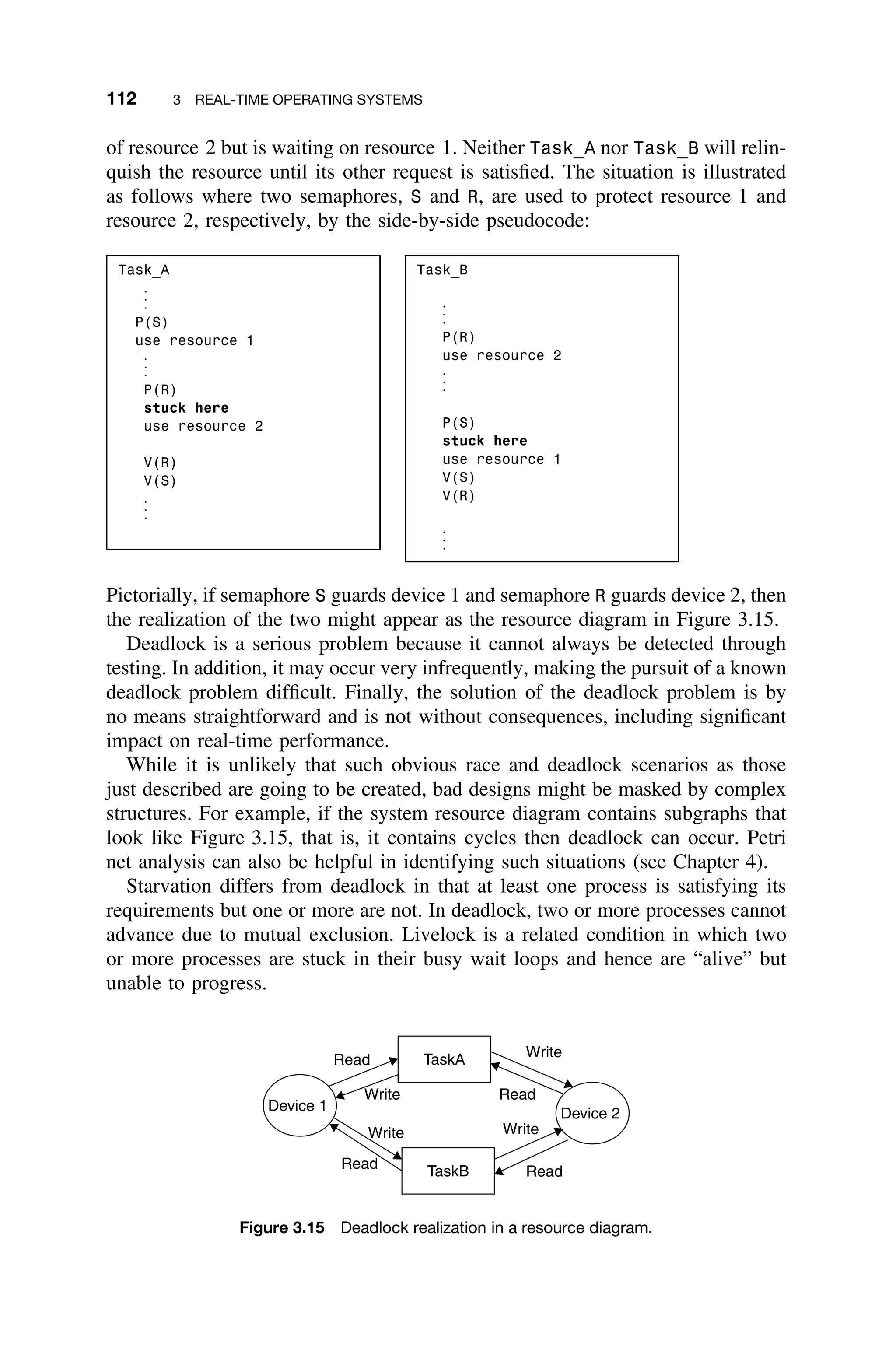
of deadlock is best illustrated by example.
For example, TASK_A requires resources 1 and 2, as does Task_B. Task_A is
in possession of resource 1 but is waiting on resource 2. Task_B is in possession](https://image.slidesharecdn.com/epdf-230618090952-bdcb6616/75/epdf-pub_real-time-systems-design-and-analysis-pdf-134-2048.jpg)
![114 3 REAL-TIME OPERATING SYSTEMS
Finally, eliminating preemption will preclude deadlock. Namely, if a low-
priority task holds a resource protected by semaphore S, and if a higher-priority
task interrupts and then waits for semaphore S, the priority inversion will cause
the high-priority task to wait forever, since the lower-priority task can never run
to release the resource and signal the semaphore. If the higher-priority task is
allowed to preempt the lower one, then the deadlock will be avoided. However,
this solution can lead to starvation in the low-priority process, as well as to nasty
interference problems. For example, what if the low-priority task had locked the
printer for output, and now the high-priority task starts printing?
Two other ways of combating deadlock are to avoid it completely by identify-
ing unsafe states using the Banker’s algorithm, or to detect it and recover from
it. Detection of deadlock is not always easy, although watchdog timers or system
monitors can be used for this purpose.
3.3.9.1 Deadlock Avoidance The best way to deal with deadlock is to avoid
it altogether. Several techniques for avoiding deadlock are available. For example,
if the semaphores protecting critical resources are implemented by mailboxes
with time-outs, then deadlocking cannot occur, but starvation of one or more
tasks is possible.
Suppose a lock refers to any semaphore used to protect a critical region.
Then the following resource-management approach is recommended to help
avoid deadlock.
1. Minimize the number of critical regions as well as minimizing their size.
2. All processes must release any lock before returning to the calling function.
3. Do not suspend any task while it controls a critical region.
4. All critical regions must be error free.
5. Do not lock devices in interrupt handlers.
6. Always perform validity checks on pointers used within critical regions.
Pointer errors are common in certain languages, like C, and can lead to
serious problems within the critical regions.
Nevertheless items 1 through 6 are difficult to achieve and other means are often
necessary to avoid deadlock.
1. The Banker’s Algorithm The Banker’s Algorithm can be used to avoid
unsafe situations that can lead to deadlock. The technique, suggested by Dijk-
stra, uses the analogy of a small-town bank, its depositors, and cash reserve
[Dijkstra68b]. In the analogy, depositors have placed money in the bank and
could potentially withdraw it all. The bank never keeps all of its deposits on
hand as cash (it invests about 95% of it). If too many depositors were to with-
draw their savings simultaneously, the bank could not fulfill the requests. The
Banker’s Algorithm was originally formulated for a single resource type, but was
soon extended for multiple resource types by Habermann [Habermann69].](https://image.slidesharecdn.com/epdf-230618090952-bdcb6616/75/epdf-pub_real-time-systems-design-and-analysis-pdf-137-2048.jpg)
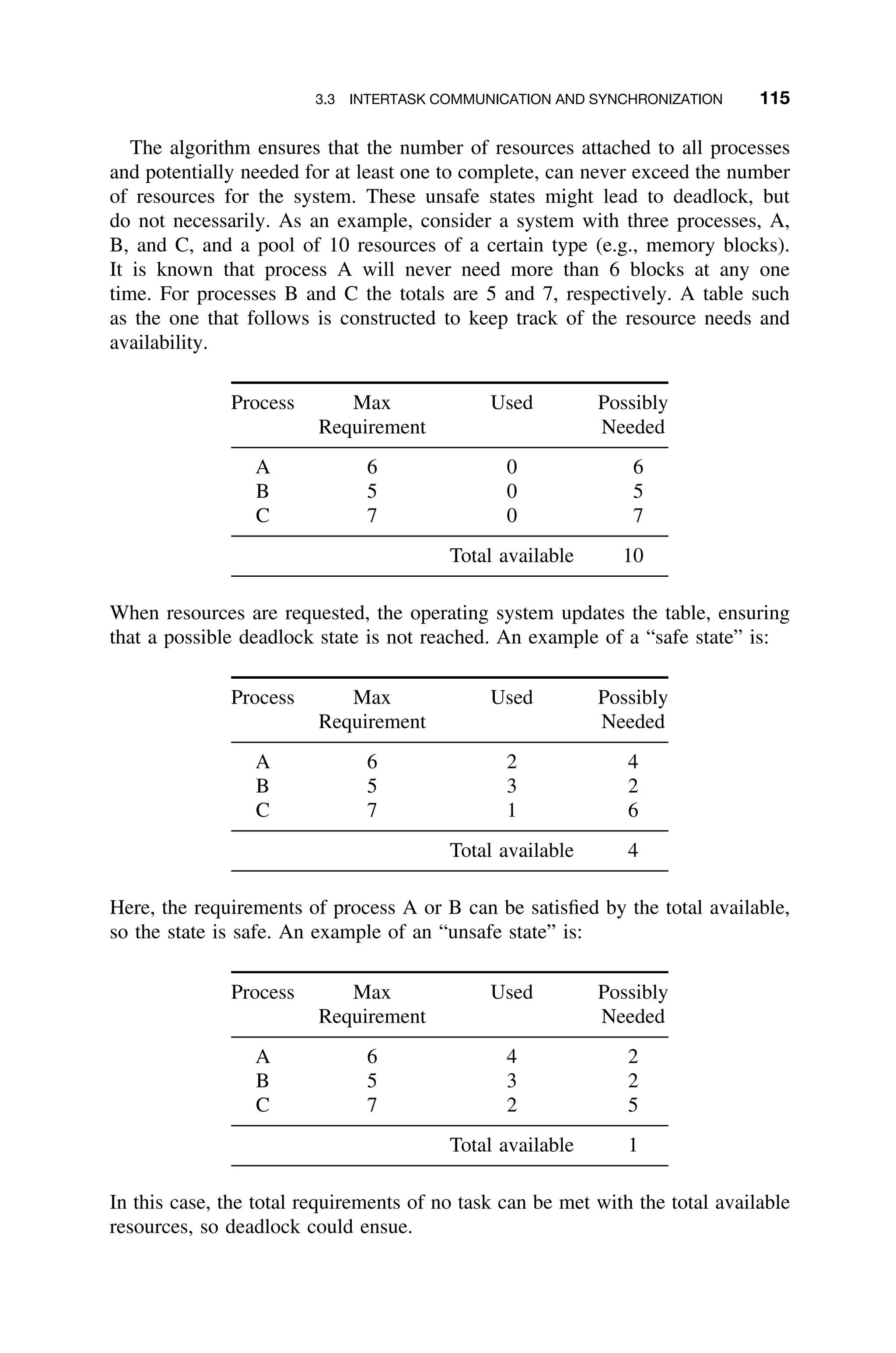
![116 3 REAL-TIME OPERATING SYSTEMS
2. Generalized Banker’s Algorithm The Banker’s Algorithm can be extended
to a set of two or more resources by expanding the table corresponding to one
resource type to one that tracks multiple resources. Formally, consider a set of
processes p1 · · · pn and a set of resources r1 · · · rm. Form the matrix max[i, j]
that represents the maximum claim of resource type j by process i. Let the
matrix alloc[i, j] represent the number of units of resource j held by process i.
Upon each request of resources of type j, cj , the resulting number of available
resources of type j if the resource is granted avail[j], is computed
avail[j] = cj −
0≤in
alloc[i, j] (3.9)
From this information, it can be determined whether or not an unsafe state will
be entered.
The procedure is as follows.
1. Update alloc[i, j], yielding alloc[i, j]
, the new alloc table.
2. Given c, max, and alloc’, compute the new avail vector.
3. Determine if there exists a pi such that max[i, j] − alloc[i, j]
≤ avail[j]
for 0 ≤ j m and 0 ≤ i n.
a. If no such pi exists, then the state is unsafe.
b. If alloc[i, j]
is for all i and j, the state is safe.
Finally, set alloc[i, j]
to 0 and deallocate all resources held by process i. For
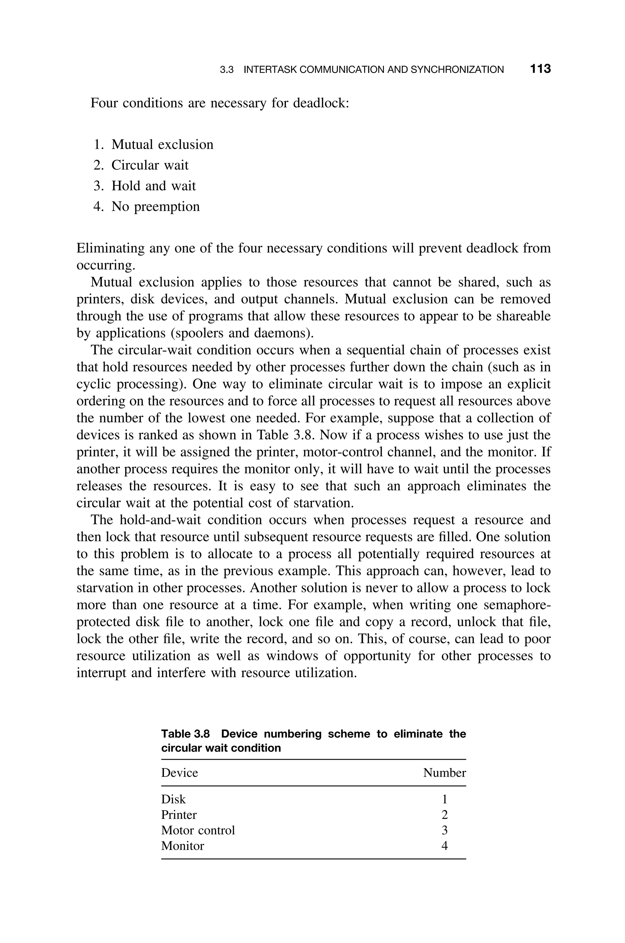
example, in the previous scenario suppose that the three processes A, B, C
share resources of type R1, R2, and R3. Resource R1, is the memory block
resource described in the previous example. Resources R2 and R3 represent other
resources, such as printers and disk drives, respectively. The initial resource table
now becomes
Process Max Requirement Used Possibly Needed
R1 R2 R3 R1 R2 R3 R1 R2 R3
A 6 3 4 0 0 0 6 3 4
B 5 3 5 0 0 0 5 3 5
C 7 2 1 0 0 0 7 2 1
Total available 10 4 5
Again, when a process requests a resource, the table is inspected to ensure
that a safe state will result in granting the request. An example of a safe state is
shown below. It is safe because at least process A can satisfy all of its resource
needs with available resources.](https://image.slidesharecdn.com/epdf-230618090952-bdcb6616/75/epdf-pub_real-time-systems-design-and-analysis-pdf-139-2048.jpg)
![118 3 REAL-TIME OPERATING SYSTEMS
t1
t2
t3
t0 t1 t2 t3 t4 t5 t6 t7 t8
Normal Execution
Blocked
Time
Critical Section
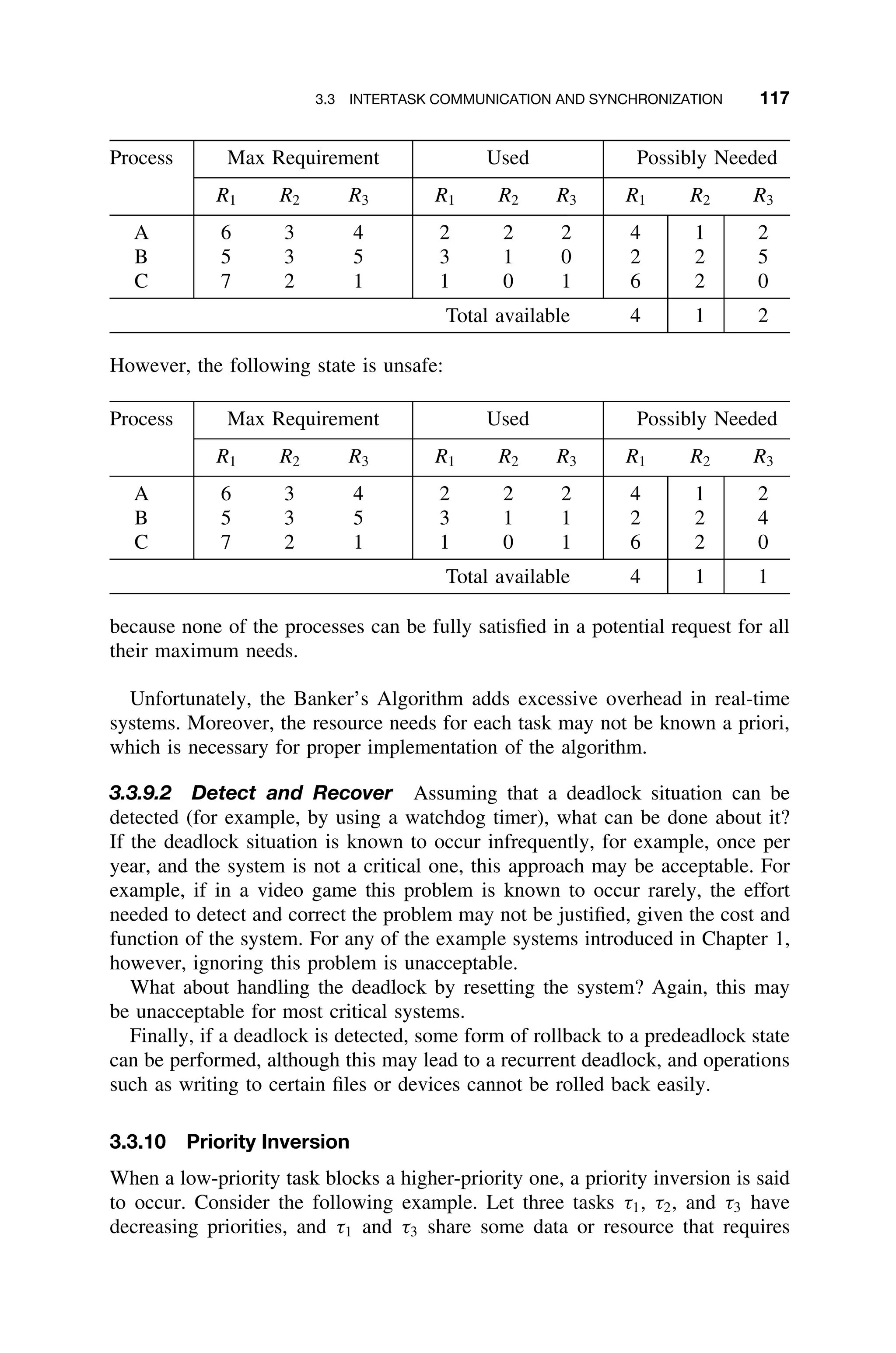
Figure 3.16 A priority inversion problem.
exclusive access, while τ2 does not interact with either of the other tasks. Access
to the critical section is done through the P and V operations on semaphore S.
Now consider the following execution scenario, illustrated in Figure 3.16. Task
τ3 starts at time t0, and locks semaphore S at time t1. At time t2, τ1 arrives and
preempts τ3 inside its critical section. At the same time, τ1 attempts to use the
shared resource by locking S, but it gets blocked, as τ3 is currently using it. At
time t3, τ3 continues to execute inside its critical section. Now if τ2 arrives at
time, t4, it preempts τ3, as it has a higher priority and does not interact with
either τ1 or τ3. The execution of τ2 increases the blocking time of τ1, as it is
no longer dependent only on the length of the critical section executed by τ3.
This event can take place with other intermediate priority tasks, and thereby can
lead to an unbounded or an excessive blocking. Task τ1 resumes its execution
at time t6 when τ3 completes its critical section. A priority inversion is said to
occur between time interval [t3, t6] during which the highest priority task τ1 has
been unduly prevented from execution by a medium-priority task. Note that the
blocking of τ1 during the periods [t3, t4] and [t5, t6] by τ3, which has the lock, is
preferable to maintain the integrity of the shared resources.
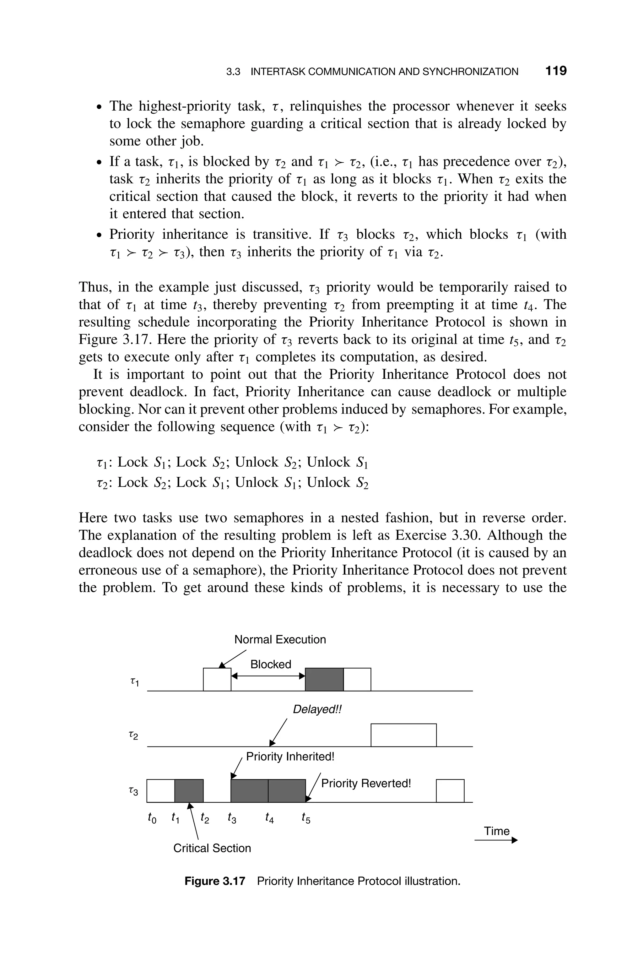
3.3.10.1 The Priority Inheritance Protocol The problem of priority inver-
sion in real-time systems has been studied intensively for both fixed-priority and
dynamic-priority scheduling. One result, the Priority Inheritance Protocol, offers
a simple solution to the problem of unbounded priority inversion.
In the Priority Inheritance Protocol the priority of tasks are dynamically changed
so that the priority of any task in a critical region gets the priority of the highest
task pending on that same critical region. In particular, when a task, τi, blocks
one or more higher-priority tasks, it temporarily inherits the highest priority of the
blocked tasks. The highlights of the protocol are:](https://image.slidesharecdn.com/epdf-230618090952-bdcb6616/75/epdf-pub_real-time-systems-design-and-analysis-pdf-141-2048.jpg)
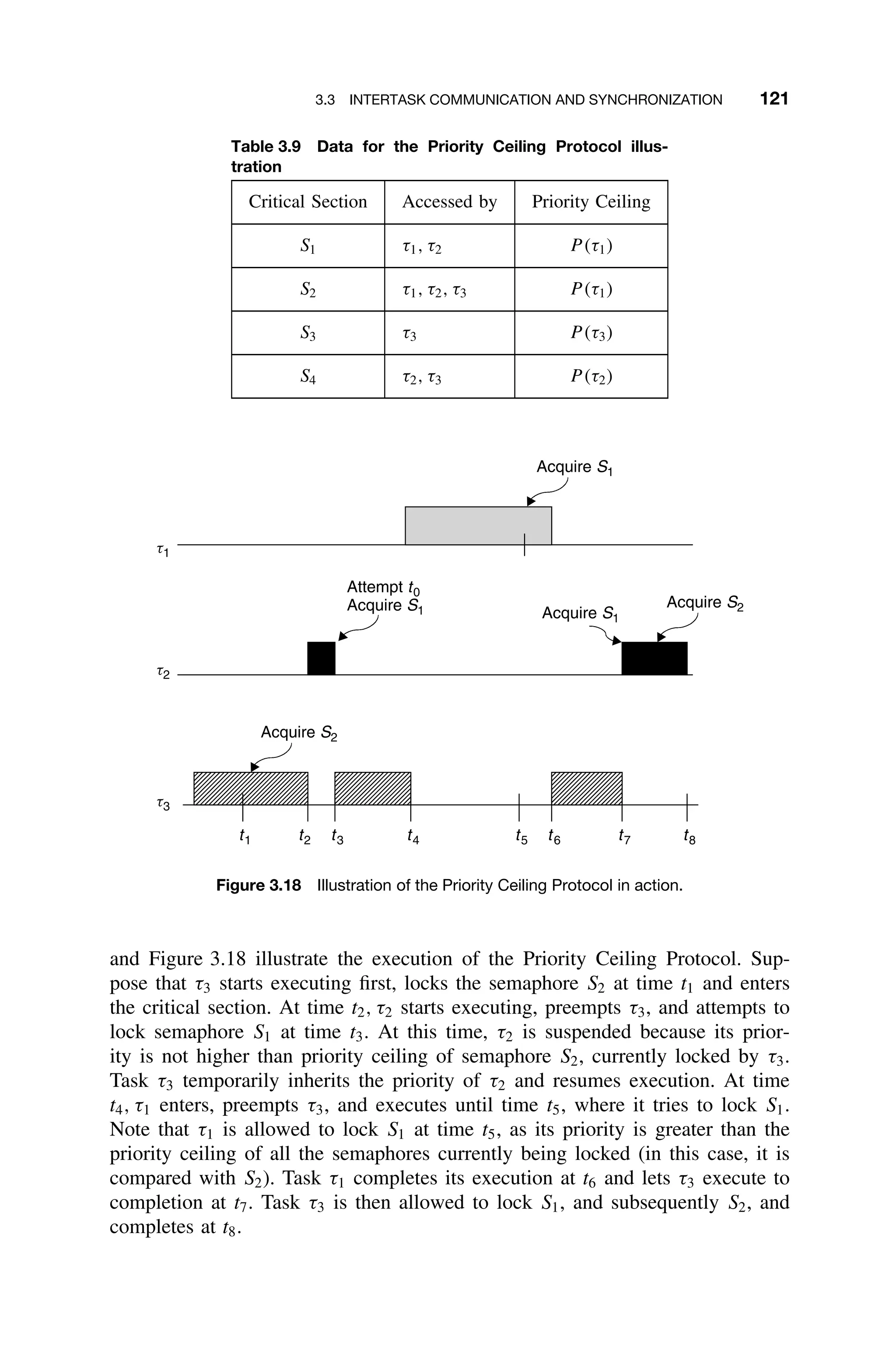
![120 3 REAL-TIME OPERATING SYSTEMS
Priority Ceiling Protocol, which imposes a total ordering on the semaphore access.
This will be discussed momentarily.
A popular commercial operating system implements the Priority Inheritance
Protocol as follows (in this case it is termed “pseudopriority inheritance”). When
process A sees that process B has the resource locked, it suspend waiting for
either (1) the resource to become unlocked, or (2) a minimal time-delay event.
When it does suspend, process A gives the remainder of its time slice to B (to
allow it to run immediately at a pseudohigher priority). If it is ready to run, B
then runs in place of A. If it is not ready to run (i.e., suspended), B and A both
are suspended to allow all other tasks to run. When A wakes up, the process is
repeated until the resource becomes unlocked.
Finally, a notorious incident of the priority inversion problem occurred in 1997
in NASA’s Mars Pathfinder Space mission’s Sojourner rover vehicle, which was
used to explore the surface of Mars. In this case the Mil-std-1553B informa-
tion bus manager was synchronized with mutexes. Accordingly a meteorological
data-gathering task that was of low priority and low frequency blocked a commu-
nications task that was of higher priority and higher frequency. This infrequent
scenario caused the system to reset. The problem would have been avoided if the
priority inheritance mechanism provided by the commercial real-time operating
system (just mentioned) had been used. But it had been disabled. Fortunately,
the problem was diagnosed in ground-based testing and remotely corrected by
reenabling the priority inheritance mechanism [Cottet02].
3.3.10.2 Priority Ceiling Protocol The Priority Ceiling Protocol extends to
the Priority Inheritance Protocol through chained blocking in such a way that no
task can enter a critical section in a way that leads to blocking it. To achieve this,
each resource is assigned a priority (the priority ceiling) equal to the priority of
the highest priority task that can use it.
The Priority Ceiling Protocol is the same as the Priority Inheritance Protocol,
except that a task, T , can also be blocked from entering a critical section if there
exists any semaphore currently held by some other task whose priority ceiling
is greater than or equal to the priority of T . For example, consider the scenario
illustrated in Table 3.9. Suppose that τ2 currently holds a lock on S2, and τ1 is
initiated. Task τ1 will be blocked from entering S1 because its priority is not
greater than the priority ceiling of S2.
As a further example, consider the three tasks with the following sequence of
operations, and having decreasing priorities:
τ1: Lock S1; Unlock S1
τ2: Lock S1; Lock S2; Unlock S2; Unlock S1
τ3: Lock S2; Unlock S2
Following the rules of assigning priority ceiling to semaphores, the priority ceil-
ings of S1 and S2 are P (τ1) and P (τ2), respectively. The following description](https://image.slidesharecdn.com/epdf-230618090952-bdcb6616/75/epdf-pub_real-time-systems-design-and-analysis-pdf-143-2048.jpg)
![134 3 REAL-TIME OPERATING SYSTEMS
For embedded systems, when the per-unit charge for commercial products is
too high, or when desired features are unavailable, or when the overhead is too
high, the only alternative is to write the real-time kernel. But this is not a trivial
task. Therefore, commercial RTOS should be considered wherever possible.
There are many commercial solutions available for real-time systems, but
deciding which one is most suitable for a given application is difficult. Many
features of embedded real-time operating systems must be considered, including
cost, reliability, and speed. But there are many other characteristics that may
be as important or more important, depending on the application. For example,
the RTOS largely resides in some form of ROM and usually controls hardware
that will not tolerate many faults; therefore, the RTOS should be fault-tolerant.
Also, the hardware needs to be able to react to different events in the system
very quickly; therefore, the operating system should be able to handle multiple
processes in an efficient manner. Finally, because of the hardware on which the
operating system has limited memory, the operating system must also require a
reasonable amount of memory in which to run.
In fact, there are so many functional and nonfunctional attributes of any com-
mercial RTOS that evaluation and comparison must be a subjective endeavor.
Some structure, however, should be used in the heuristic decision-making. Using
a standard set of criteria provides such structure [Laplante04].
3.4.15 Selecting Real-Time Kernels
From a business and technical perspective the selection of a commercial real-time
operating system represents a potential make-or-break decision. It is therefore
imperative that a rigorous set of selection criteria be used. The following are
desirable characteristics for real-time systems:5
ž Timeliness
ž Design for survival under peak load
ž Predictability
ž Fault-tolerance
ž Maintainability [Buttazzo00]
Therefore the selection criteria should reflect these desiderata. Unfortunately,
unless a comprehensive experience base exists using several alternative commer-
cial RTOS in multiple, identical application domains, there are only two ways
to objectively determine the fitness of a product for a given application. The
first is to rely on third-party reports of success or failure. These abound and are
published widely on the Web. The second is to compare alternatives based on
the manufacturer’s published information from brochures, technical reports, and
Web sites. The following discussion presents an objective apples-to-apples tech-
nique for comparing commercial RTOS based on marketing information. This
5
This discussion is adapted from [Laplante04].](https://image.slidesharecdn.com/epdf-230618090952-bdcb6616/75/epdf-pub_real-time-systems-design-and-analysis-pdf-157-2048.jpg)
![3.4 MEMORY MANAGEMENT 135
technique can be used, however, in conjunction with supplemental information
from actual experience and third-party reports.
Consider thirteen selection criteria, m1 · · · m13, each having a range mi ∈ [0, 1]
where unity represents the highest possible satisfaction of the criterion and zero
represents complete nonsatisfaction.
1. The minimum interrupt latency, m1, measures the time between the occur-
rences of hardware interrupt and when the interrupt’s service routine
begins executing. A low value represents relatively high interrupt latency,
while a high value represents a low latency. This criterion is impor-
tant because, if the minimum latency is greater than that required by
the embedded system, a different operating system must be selected.
2. This criterion, m2, defines the most processes the operating system can
simultaneously support. Even though the operating system can support
a large number of tasks, this metric may be further limited by available
memory. This criterion is important for systems that need numerous simul-
taneous processes. A relatively high number of tasks supported would
result in m2 = 1, while few task supported would suggest a lower value
for m2.
3. Criterion m3 specifies the system memory required to support the operat-
ing system. It does not include the amount of additional memory required
to run the system’s application software. Criterion m3 = 1 suggests a min-
imal memory requirement, while m3 = 0 would represent a larger memory
requirement.
4. The scheduling mechanism criterion, m4, enumerates whether preemptive,
round-robin, or some other task-scheduling mechanism is used by the
operating system. If many mechanisms were supported, then a high value
would be assigned to m4.
5. Criterion m5 refers to the available methods the operating system has to
allow processes to communicate with each other. Among possible choices
are mutual exclusion (mutexes), binary and counting semaphores, POSIX
pipes, message queues, shared memory, FIFO buffers, control sockets,
and signals and scheduling. Each mechanism has advantages and disad-
vantages, and they have been discussed. Let m5 = 1 if the RTOS provides
all desired scheduling mechanisms. A lower value for m5 implies that
fewer scheduling mechanisms are available.
6. Criterion m6 refers to the after-sale support a company puts behind its
product. Most vendors offer some sort of free technical support for a
short period of time after the sale, with the option of purchasing additional
support if required. Some even offer on-site consultation. A high value
might be assigned to a strong support program, while m6 = 0 if no support
is provided.
7. Application availability, m7, refers to the amount of software available
(either that ships with the operating system or is available elsewhere)](https://image.slidesharecdn.com/epdf-230618090952-bdcb6616/75/epdf-pub_real-time-systems-design-and-analysis-pdf-158-2048.jpg)
![136 3 REAL-TIME OPERATING SYSTEMS
to develop applications to run on the operating system. For example,
RTLinux is supported by the GNU’s suite of software, which includes the
gcc C compiler and many freely available software debuggers, and other
supporting software. This is an important consideration, especially when
using an unfamiliar operating system. Let m7 = 1 if a large amount of soft-
ware were available, while 0 would mean that little or none was available.
8. Criterion m8 refers to the different processors that the operating system
supports. This is important in terms of portability and compatibility with
off-the-shelf hardware and software. This criterion also encompasses the
range of peripherals that the operating system can support, such as video,
audio, SCSI, and such. A high value for the criterion represents a highly
portable and compatible RTOS.
9. Criterion m9 refers to whether the code of the operating system will be
available to the developer, for tweaking or changes. The source also gives
insight to the RTOS architecture, which is quite useful for debugging
purposes and systems integration. Setting m9 = 1 would suggest open
source code or free source code, while a lower value might be assigned
in proportion to the purchase price of the source code. Let m9 = 0 if the
source code were unavailable.
10. Criterion m10 refers to the time it takes for the kernel to save the context
when it needs to switch from one task to another. A relatively fast context
switch time would result in a higher value for m10.
11. This criterion is directly related to the cost of the RTOS alone. This is
critical because for some systems, the RTOS cost may be disproportion-
ately high. In any case, a relatively high cost would be assigned a very
low value, while a low cost would merit a higher value for m11.
12. This criterion, m12, rates which development platforms are available. In
other words, it is a listing of the other operating systems that are com-
patible with the given RTOS. A high value for m12 would represent wide
compatibility, while a lower m12 would indicate compatibility with only
one platform.
13. This criterion, m13, is based on a listing of what networks and network
protocols are supported by the given RTOS. This would be useful to know
because it rates what communication methods the software running on this
operating system would be able to use to communicate to other comput-
ers within the same computer network. A high value for the criterion
represents a relatively large number of networks supported.
Recognizing that the importance of individual criteria will differ depending on
the application, a weighting factor, wi ∈ [0, 1], will be used for each criterion
mi, where unity is assigned if the criterion has highest importance, and zero if
the criterion is unimportant for a particular application. Then a fitness metric,](https://image.slidesharecdn.com/epdf-230618090952-bdcb6616/75/epdf-pub_real-time-systems-design-and-analysis-pdf-159-2048.jpg)
![3.4 MEMORY MANAGEMENT 137
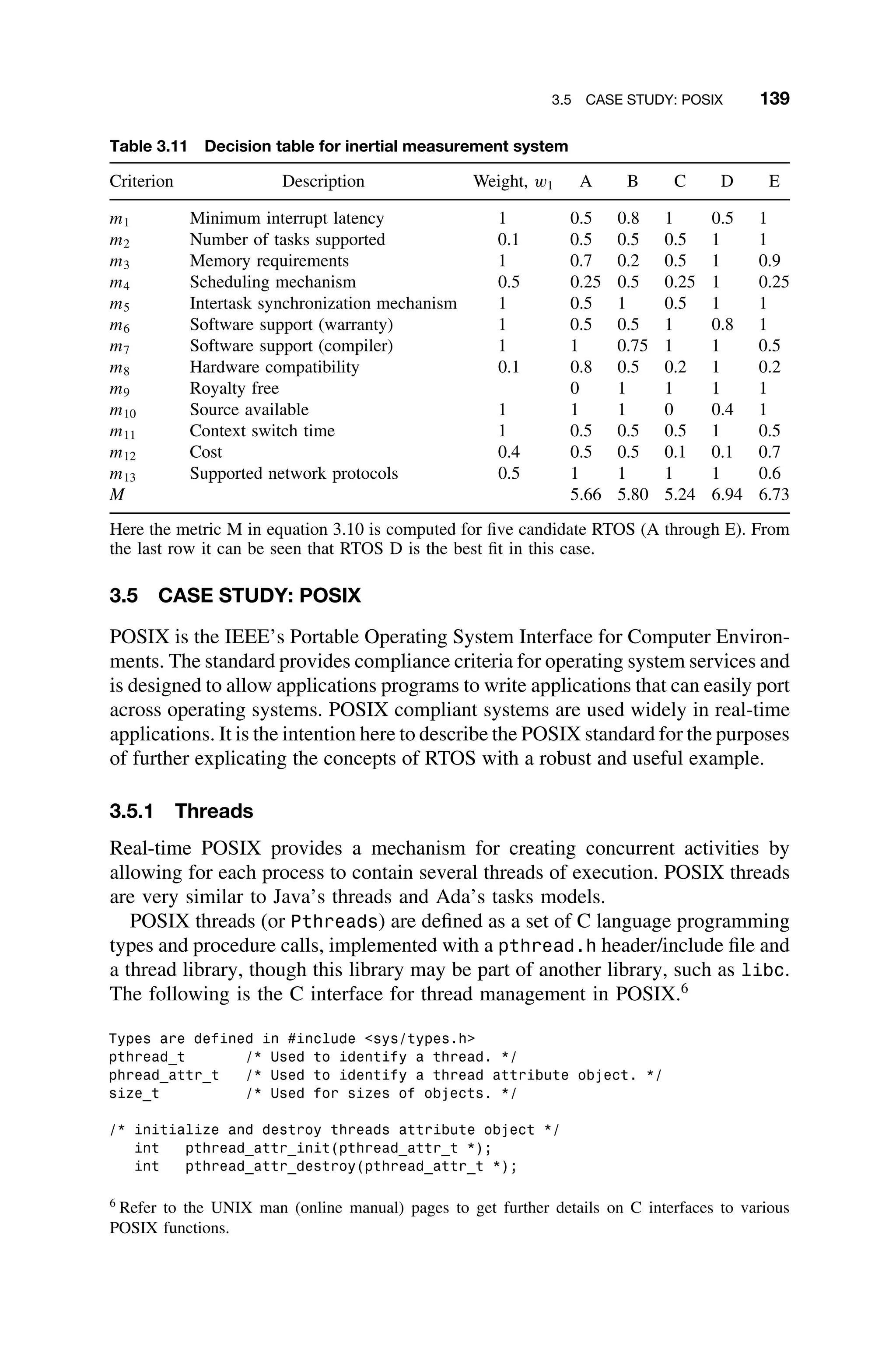
M ∈ [0, 13], is formed as
M =
13
i=1
wimi (3.10)
Clearly, a higher value of M means that the RTOS is well suited to the appli-
cation, while a lower value means that the RTOS is not well suited for the
application.
While selection of the values for mi and wi will be subjective for any given
RTOS and any given application, the availability of this heuristic metric provides
a handle for objective comparison, historical perspective, and other uses.
3.4.15.1 A Case Study in Selecting a Commercial Real-Time Operating
System A typical commercial RTOS is now examined based on the criteria
introduced. Although the data are real, the manufacturer name is omitted, as the
intention is not to imply a recommendation of any product.
The following assumptions are made:
ž For all the sample RTOS, assume that the calculations for the number of
interrupt, the minimum time that it takes, and other system analysis based
on the metrics chosen are performed under the same conditions, that is,
sampling, time constraints, and number of processors.
ž Maximum or minimum of tasks refers to the operating system object, such
as the memory management unit (MMU), device drivers, and other sys-
tem tasks.
ž Assume that interrupt refers to “hardware interrupt.” “Software interrupts,”
together with hardware interrupts and other vectoring mechanisms provided
by the processor, are referred to as “exception handling.”
ž Thread switching latency time is equivalent to the measurement of context
switching latency time.
In the cases where a criterion value can be assigned, this is done. Where the
criteria are “processor dependent” or indeterminate, absent a real application,
assignment of a rating is postponed, and a value of * is given. This “uncertain”
value is fixed at the time of application analysis. Note too that the values between
tables need to be consistent. So, for example, if a 6-microsecond latency yields
m1 = 1 for RTOS X, the same 6-microsecond latency should yield m1 = 1 for
RTOS Y.
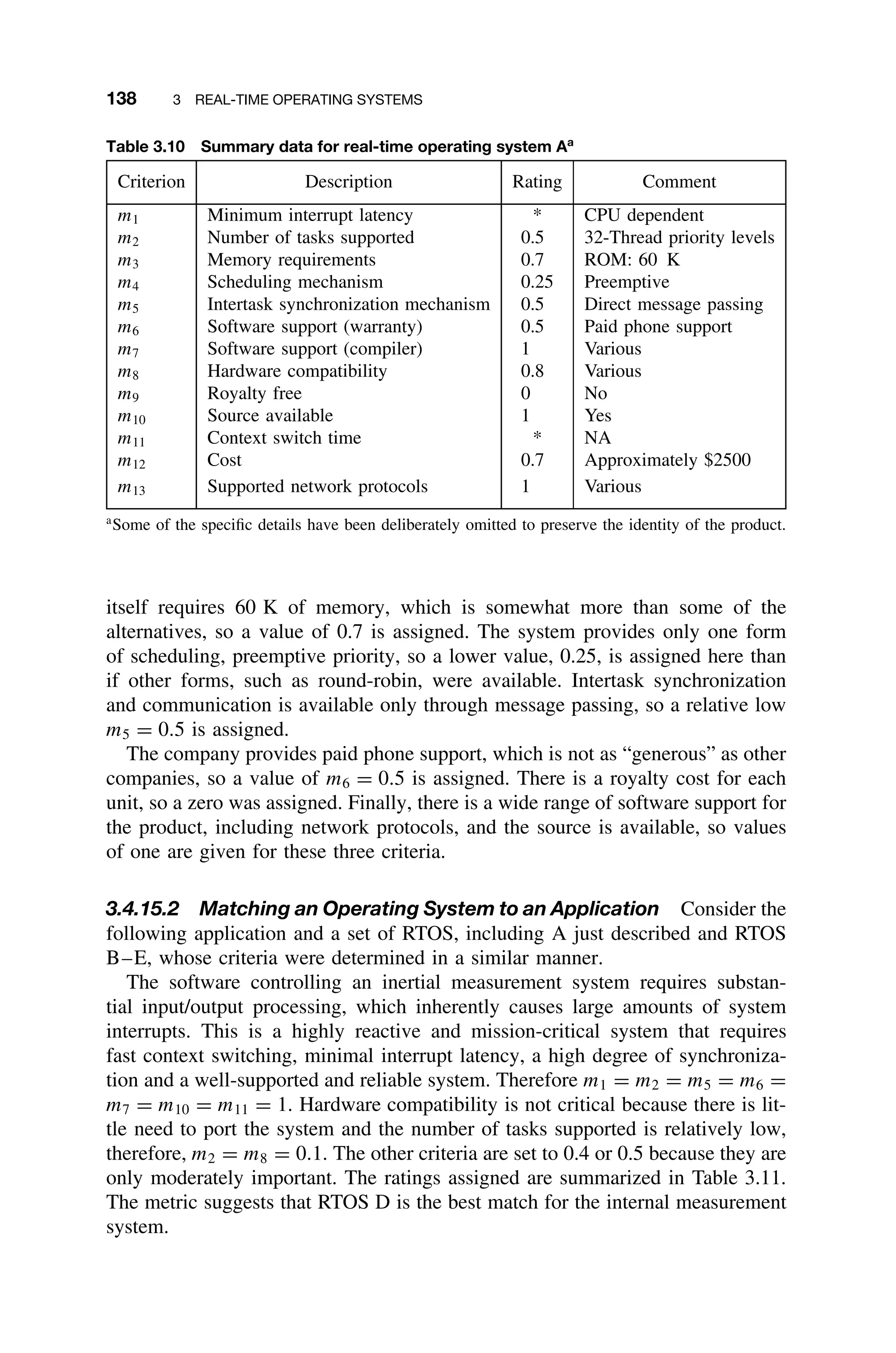
Consider commercial RTOS A. Table 3.10 summarizes the criteria and ratings,
which were based on the following rationale. The product literature indicated
that the minimum interrupt latency is CPU dependent, therefore a * value is
assigned here (which will be later resolved as 0.5 for the purposes of evaluating
the metric). Context switch time is not given, and so a * is also indicated.
The RTOS supports 32-thread priority levels, but it is not known if there is a
limit on the total number of tasks, so a value of 0.5 is assigned. The RTOS](https://image.slidesharecdn.com/epdf-230618090952-bdcb6616/75/epdf-pub_real-time-systems-design-and-analysis-pdf-160-2048.jpg)
![3.5 CASE STUDY: POSIX 141
Table 3.12 POSIX naming scheme
Routine Prefix Functional Group
pthread Threads themselves and miscellaneous subroutines
pthread attr Thread attributes objects
pthread mutex Mutexes
pthread mutexattr Mutex attributes objects
pthread cond Condition variables
pthread condattr Condition attributes objects
pthread key Thread-specific data keys
{
pthread_t thread[5];
pthread_attr_t attribute;
int errorcode,counter, status;
char *message=TestPrint;
/* Initialize and set thread detached attribute */
pthread_attr_init(attribute);
pthread_attr_setdetachstate(attribute, PTHREAD_CREATE_JOINABLE);
for(counter=0;counter5;counter++)
{
printf(I am creating thread %dn, counter);
errorcode = pthread_create(thread[counter],
attribute,(void*)message_printer_function,(void*)message);
if (errorcode)
{
printf(ERROR happened in thread creation);
exit(-1);
}
}
/* Free attribute and wait for the other threads */
pthread_attr_destroy(attribute);
for(counter=0;counter5;counter++)
{
errorcode = pthread_join(thread[counter], (void **)status);
if (errorcode)
{
printf(ERROR happened in thread join);
exit(-1);
}
printf(Completed join with thread %dn,counter);
/*printf(Completed join with thread %d status= %dn,counter, status);*/
}
pthread_exit(NULL);
}](https://image.slidesharecdn.com/epdf-230618090952-bdcb6616/75/epdf-pub_real-time-systems-design-and-analysis-pdf-164-2048.jpg)
![146 3 REAL-TIME OPERATING SYSTEMS
int mq_notify(mqd_t mqdes, const struct sigevent *notification);
/* Notifies a process or thread that a message is available in the queue. */
The following example illustrates sending and receiving messages between
two processes using a message queue [Marshall96]. The following two programs
should be compiled and run at the same time to illustrate the basic principle of
message passing:
message_send.c Creates a message queue and sends one message to
the queue.
message_rec.c Reads the message from the queue.
The full code listing for message_send.c is as follows:
#include sys/types.h
#include sys/ipc.h
#include sys/msg.h
#include stdio.h
#include string.h
#define MSGSZ 128
/* Declare the message structure. */
typedef struct msgbuf {
long mtype;
char mtext[MSGSZ];
} message_buf;
main()
{
int msqid;
int msgflg = IPC_CREAT | 0666;
key_t key;
message_buf sbuf;
size_t buf_length;
/* Get the message queue id for the name 1234, which was created by the
server. */
key = 1234;
(void) fprintf(stderr, nmsgget: Calling msgget(%#lx, %#o)n, key, msgflg);
if ((msqid = msgget(key, msgflg )) 0)
{
perror(msgget);
exit(1);
}
else
(void) fprintf(stderr,msgget: msgget succeeded: msqid = %dn, msqid);
/* We’ll send message type 1 */
sbuf.mtype = 1;
(void) fprintf(stderr,msgget: msgget succeeded: msqid = %dn, msqid);
(void) strcpy(sbuf.mtext, Did you get this?);
(void) fprintf(stderr,msgget: msgget succeeded: msqid = %dn, msqid);](https://image.slidesharecdn.com/epdf-230618090952-bdcb6616/75/epdf-pub_real-time-systems-design-and-analysis-pdf-169-2048.jpg)
![3.5 CASE STUDY: POSIX 147
buf_length = strlen(sbuf.mtext) + 1 ;
/* Send a message. */
if (msgsnd(msqid, sbuf, buf_length, IPC_NOWAIT) 0) {
printf (%d, %d, %s, %dn, msqid, sbuf.mtype, sbuf.mtext, buf_length);
perror(msgsnd);
exit(1);
}
else
printf(Message: %s Sentn, sbuf.mtext);
exit(0);
}
The essential points to note here are:
ž The Message queue is created with a basic key and message flag
msgflg = IPC_CREAT | 0666 -- create queue and make it read and
appendable by all.
ž A message of type (sbuf.mtype) 1 is sent to the queue with the message
“Did you get this?”
Receiving the preceding message as sent using message_send program is
illustrated below. The full code listing for message_send.c’s companion pro-
cess, message_rec.c is as follows:
#include sys/types.h
#include sys/ipc.h
#include sys/msg.h
#include stdio.h
#define MSGSZ 128
/* Declare the message structure. */
typedef struct msgbuf {
long mtype;
char mtext[MSGSZ];
} message_buf;
main()
{
int msqid;
key_t key;
message_buf rbuf;
/* Get the message queue id for the name 1234, which was created by the
server. */
key = 1234;
if ((msqid = msgget(key, 0666)) 0) {
perror(msgget);
exit(1);
}](https://image.slidesharecdn.com/epdf-230618090952-bdcb6616/75/epdf-pub_real-time-systems-design-and-analysis-pdf-170-2048.jpg)
![156 3 REAL-TIME OPERATING SYSTEMS
Stack
Heap
Data
Text
Stack
Heap
Data
Text
Pageable
Locked
char buf[100] char buf[100]
Before mlock Call After mlock(buf, 100) Call
Figure 3.25 mlock operation.
calling munlockall unlocks the memory that has been locked with mlock. It is
not possible to lock memory for all of a small section of code, then unlock it.
Memory locking is a global technique that should not be performed by small,
transient sections of code. In general, once a memory is locked, it should be
locked down until the application is out of “real-time mode.” The function mlock
can cause a segmentation fault if an address is passed to it where there is not
any memory for executable code.
As can be seen from this example, memory locking decreases execution times
for the locked modules and, more importantly, can be used to guarantee execu-
tion time. At the same time, it makes fewer pages available for the application,
encouraging contention.
3.6 EXERCISES
3.1 For the sample real-time systems described in Chapter 1, discuss which real-time
architecture is most appropriate.
(a) Inertial measurement system
(b) Nuclear monitoring system
(c) Airline reservations system
(d) Pasta sauce bottling system
(e) Traffic light control
Make whatever assumptions you like, but document them.
3.2 Should a task be allowed to interrupt itself? If it does, what does this mean?
3.3 What criteria are needed to determine the size of the run-time stack in a multiple-
interrupt system? What safety precautions are necessary?
3.4 Identify some of the limitations of existing commercial real-time kernels for the
development of different mission- and safety-critical applications.
3.5 What are the desirable features that a system should have to provide for predictabil-
ity in time-critical applications?
3.6 Discuss the difference between static and dynamic, on-line and off-line, optimal,
and heuristic scheduling algorithms.](https://image.slidesharecdn.com/epdf-230618090952-bdcb6616/75/epdf-pub_real-time-systems-design-and-analysis-pdf-179-2048.jpg)
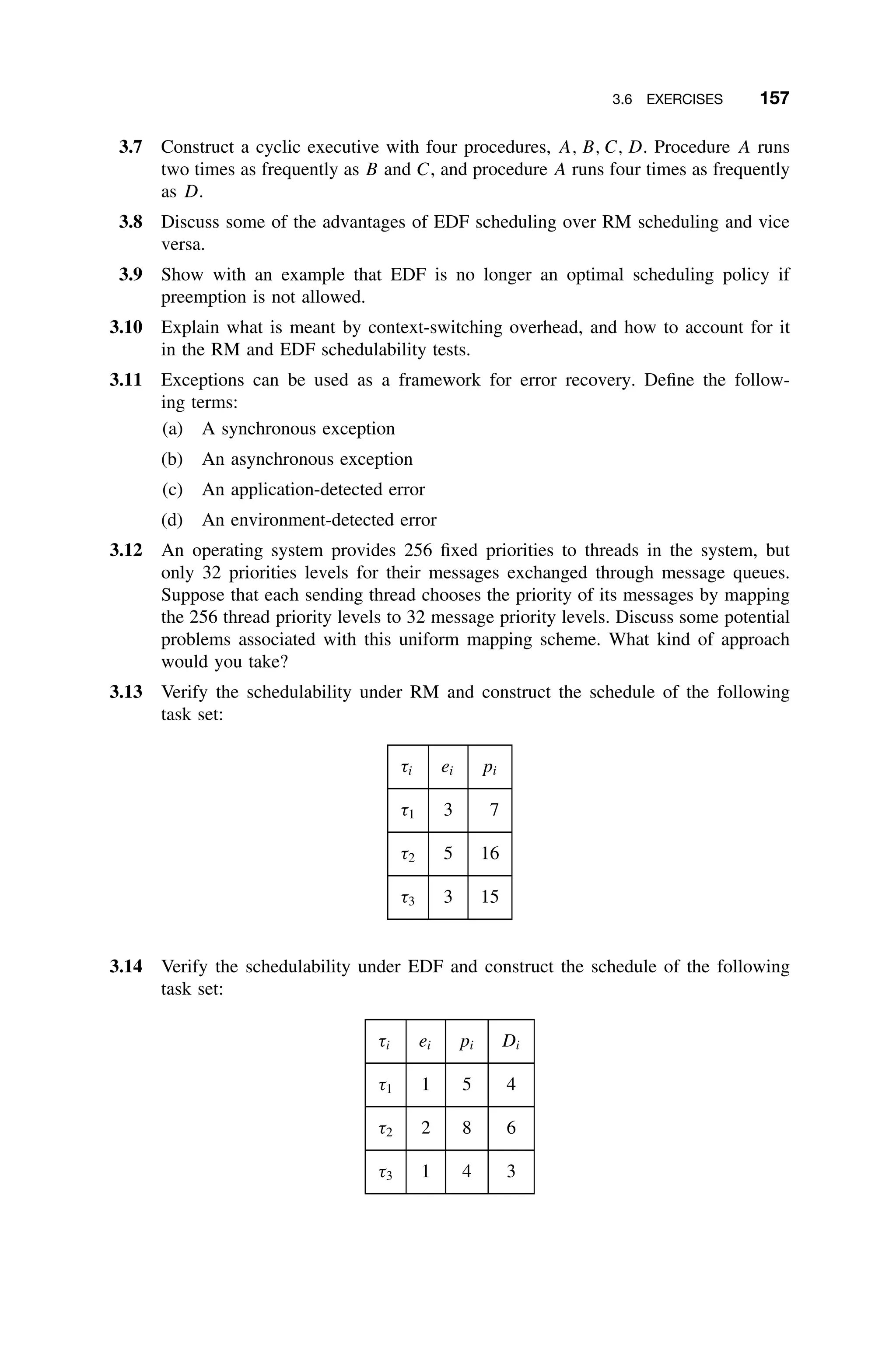
![158 3 REAL-TIME OPERATING SYSTEMS
3.15 Give two different explanations why the following periodic tasks are schedulable
by the RM algorithm.
τi ei pi
τ1 0.8 2
τ2 1.4 4
τ3 2 8
3.16 The following system of periodic tasks is scheduled and executed according to a
cyclic schedule. Draw an execution trace (timeline) showing two occurances of
each task.
τi ei pi
τ1 1 8
τ2 4 15
τ3 3 20
τ4 8 22
3.17 Verify the schedulability under EDF, and construct the EDF schedule of the fol-
lowing task set in the interval (0,20).
τi ri ei pi Di
τ1 0 2 8 6
τ2 1 2 6 5
τ3 0 4 12 10
3.18 Consider the following tasks with their resource requirements given as:
(a) τ1 = (10, 4, 1; [A; 1]), where the task executes for two time units, then re-
quests the resource A.
(b) τ2 = (7, 4, 2; [A; 1][B; 1]), where the task executes for one time unit, then
requests the resource A and then B.
(c) τ3 = (4, 4, 3; [B; 1][C; 1]), where the task executes for one time unit, then
requests the resource B and then C.](https://image.slidesharecdn.com/epdf-230618090952-bdcb6616/75/epdf-pub_real-time-systems-design-and-analysis-pdf-181-2048.jpg)
![3.6 EXERCISES 159
(d) τ4 = (0, 11, 4; [A; 5[B; 2]][C; 1]), where the task executes for two time units,
then requests the resource A and holds it for one time unit and makes a nested
request for resource B, and then requests C.
Here, the notation τ1 = (ri, ei, [R, t]) represents that the task i is released at time
ri, has execution time ei, priority πi, and the critical section [R; t] for the resource
R and the execution time t. Also note that the representation [R; t[S; w]] denotes
the nested critical sections, that is, that the usage of resource R in turn includes
the usage of resource S, and time t includes the time w of the critical section S.
Construct the schedule for the system using (a) the Priority Inheritance Protocol,
(b) the Priority Ceiling Protocol.
3.19 What effect would size N of a ring buffer have on its performance? How would
you determine the optimal size?
3.20 For a machine you are familiar with, discuss whether the counting semaphore
implementation given in this chapter has any critical-region problems. That is, can
the semaphore itself be interrupted in a harmful way?
3.21 Why is it not wise to disable interrupts before the while statement in the binary
semaphore, P(S)?
3.22 Discuss the problems that can arise if the test and set in the P(S) operation are
not atomic. What could happen if the simple assignment statement in the V(S)
operation were not atomic?
3.23 Rewrite the save and restore routines assuming that eight general register
(R0–R7) and the program counter are to be saved on a stack. Do this for
(a) 0-address machine
(b) 1-address machine
(c) 3-address machine
3.24 Rewrite the save and restore routines so that they save and restore to the
head and tail of a ring buffer, respectively.
3.25 Rewrite the save and restore routines in 2-address code, assuming block move
(BMOVE) and restore (BRESTORE) instructions are available. Make the necessary
assumptions about the format of the instructions.
3.26 Rewrite the save and restore routines in the language of your choice so that
they employ the push and pop procedures.
3.27 Write a pseudocode algorithm that allocates pages of memory on request. Assume
that 100 pages of size 1 megabyte, 2 megabytes, and 4 megabyte are available. The
algorithm should take the size of the page requested as an argument, and return a
pointer to the desired page. The smallest available page should be used, but if the
smallest size is unavailable, the next smallest should be used.
3.28 Write a pseudocode algorithm compacting 64 megabytes of memory that is divided
into 1-megabyte pages. Use a pointer scheme.
3.29 A real-time system has a fixed number of resources of types A, B, and C. There
are five tasks in the system, and the maximum amount of resources A, B, and
C needed for each task is known. Implement a banker’s algorithm scheme in the
language of your choice.](https://image.slidesharecdn.com/epdf-230618090952-bdcb6616/75/epdf-pub_real-time-systems-design-and-analysis-pdf-182-2048.jpg)
![162 4 SOFTWARE REQUIREMENTS ENGINEERING
Preliminary
Study
Requirements
Validation
Requirements
Definition
Requirements
Elicitation
Feasibility
Report Domain
Model
Requirements
Document
Definition of
Requirements
Requirements
Specification
Figure 4.1 The requirements-engineering process depicting documentation in rectangles and
activities in smoothed rectangles. Adapted from Sommerville [Sommerville00].
constraints imposed upon the system. One of the major deliverables of the pre-
liminary study is a feasibility report that may advise discontinuing development
of the software product. Most of the time this will not be the case, and the
preliminary study will be followed by requirements elicitation.
Requirements elicitation involves gathering requirements through a variety of
techniques that may include stakeholder interviews and questionnaires, focus
groups, workshops, and prototyping. While requirements can be expressed in
many forms ranging from standard text through mathematical formalisms, it is
usual for requirements to be represented in the form of a domain model, that
is, a model of the problem domain that may include such artifacts as use cases,
entity-relationship diagrams, or context diagrams.
The next stage is requirements definition. It is important to define, as precisely
as possible, each of the captured requirements so that they can be analyzed
for completeness, noncontradiction, and correctness in the validation stage. The
overall outcome of this process is a requirements document containing a software
requirements specification (SRS), which is a description of the features, behav-
iors, and constraints of the final system. Precise software specifications provide
the basis for analyzing the requirements, validating that they are the stakeholder’s
intentions, defining what the designers have to build, and verifying that they have
done so correctly.
4.2 TYPES OF REQUIREMENTS
While there are a number of useful taxonomies of requirements, the most estab-
lished being the simple functional versus nonfunctional classification, the standard
scheme for real-time systems is defined by IEEE Standard [IEEE830]. Standard
830 [IEEE98] defines the following kinds of requirements:
1. Functional
2. External interfaces](https://image.slidesharecdn.com/epdf-230618090952-bdcb6616/75/epdf-pub_real-time-systems-design-and-analysis-pdf-185-2048.jpg)
![164 4 SOFTWARE REQUIREMENTS ENGINEERING
users to be supported. The dynamic requirements might include the number of
transactions and tasks and the amount of data to be processed within certain time
periods for both normal and peak workload conditions.
Logical database requirements include the types of information used by various
functions, such as frequency of use, accessing capabilities, data entities and their
relationships, integrity constraints and data-retention requirements. Design con-
straint requirements are related to standards compliance and hardware limitations.
Lastly, software system attribute requirements include reliability, availability,
security, maintainability, and portability.
It is worth observing that the conventional nomenclature for functional versus
nonfunctional requirements is unfortunate; however, because the terms functional/
nonfunctional seem inappropriate for real-time systems. A more logical taxonomy
would include a classification of behavior observable via execution and that which
is not observable via execution (e.g., maintainability, portability).
4.3 REQUIREMENTS SPECIFICATION FOR REAL-TIME SYSTEMS
There appears to be no particularly dominant approach for specification of real-
time applications [Bucci95]. In general, it seems that real-time systems engineers
tend to use one or a combination of the following approaches:
ž Top-down process decomposition or structured analysis.
ž Object-oriented approaches.
ž Program description languages (PDL) or pseudocode.
ž High-level functional specifications that are not further decomposed.
ž Ad hoc techniques, including simple natural language and mathematical
description, and are always included in virtually every system specification.
There are three general classifications of specification techniques; informal,
formal, and semiformal. Formal methods have a rigorous, mathematical basis.
A small sampling of these approaches is discussed in the next section. A
requirements specification technique is informal if it cannot be completely
transliterated into a rigorous mathematical notation and associated rules.
Informal specifications, for example, flowcharting, have little or no underlying
mathematical structure, therefore, they cannot be properly analyzed. All that
can be done with informal specifications is to find counterexamples of where
the system fails to meet the requirements or where there are conflicts. This
is simply not good enough for real-time systems where formal substantiation
of performance characteristics of requirements is necessary. Approaches to
requirements specification that defy classification as either formal or informal
are sometimes called semiformal. Semiformal approaches, while not appearing
to be mathematically based, might be. For example, some contend that Unified
Modeling Language (UML) is semiformal because the Statechart is formal and
other metamodeling techniques it employs have a pseudomathematical basis.](https://image.slidesharecdn.com/epdf-230618090952-bdcb6616/75/epdf-pub_real-time-systems-design-and-analysis-pdf-187-2048.jpg)
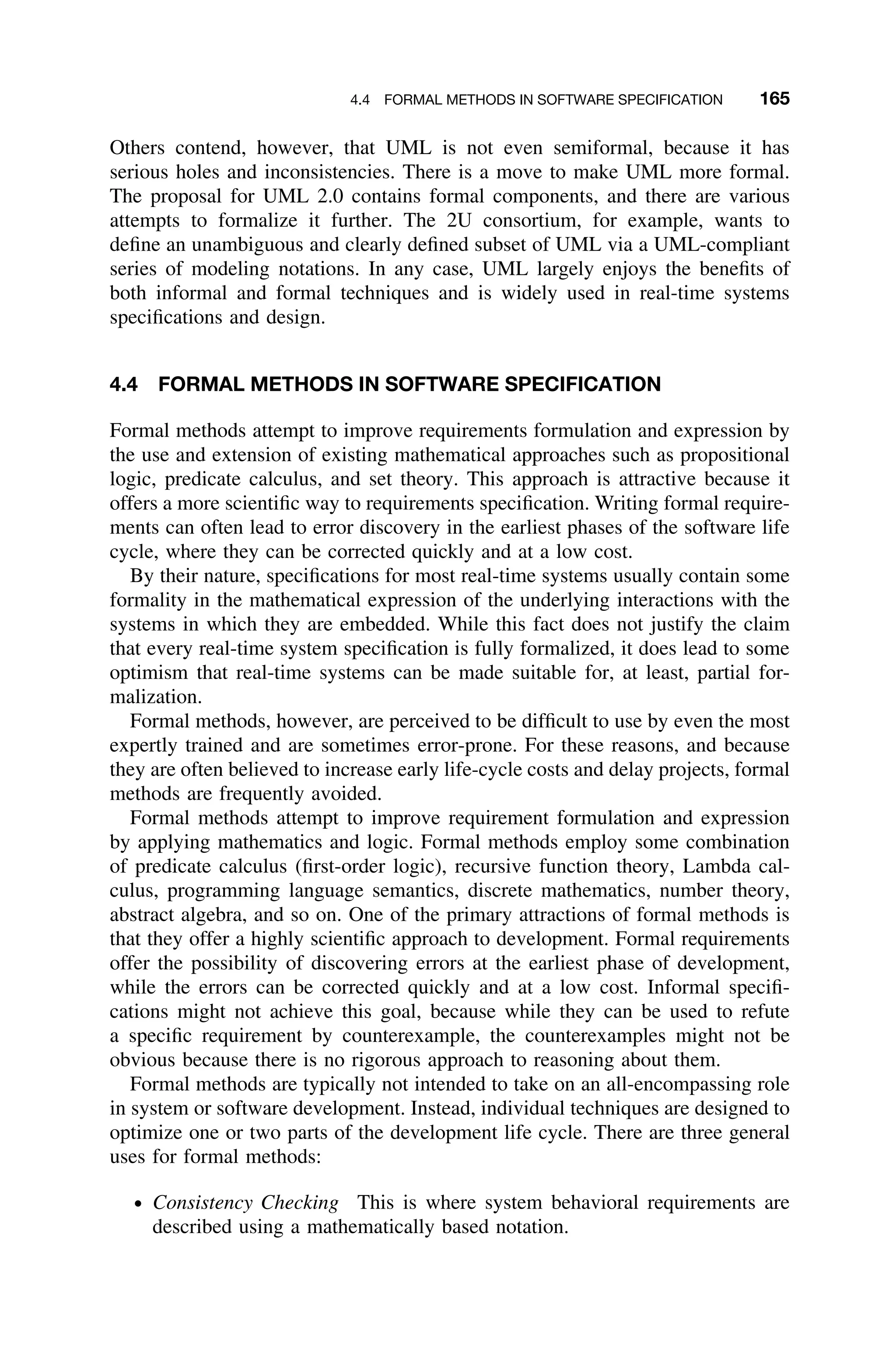
![166 4 SOFTWARE REQUIREMENTS ENGINEERING
ž Model Checking State machines are used to verify whether a given property
is satisfied under all conditions.
ž Theorem Proving Here, axioms of system behavior are used to derive a
proof that a system will behave in a given way.
Formal methods also offer opportunities for reusing requirements. Embedded
systems are often developed as families of similar products, or as incremental
redesigns of existing products. For the first situation, formal methods can help
identify a consistent set of core requirements and abstractions to reduce duplicate
engineering effort. For redesigns, having formal specifications for the existing
system provides a precise reference for baseline behavior, and provides a way to
analyze proposed changes [Bowen95].
As a simple example of the use of formal methods, consider the following
excerpt from the Software Requirements Specification for the nuclear monitor-
ing system:
1.1 If interrupt A arrives, then task B stops executing.
1.2 Task A begins executing upon arrival of interrupt A.
1.3 Either Task A is executing and Task B is not, or Task B is executing
and Task A is not, or both are not executing.
These requirements can be formalized by rewriting each in terms of their com-
ponent propositions, namely:
p: interrupt A arrives
q: task B is executing
r: task A is executing
Then rewriting the requirements using these propositions and logical connec-
tives yields:
1.1 p ⇒ ¬q
1.2 p ⇒ r
1.3 (r ∧ ¬q) ∨ (q ∧ ¬r) ∨ (¬q ∧ ¬r)
Notice the difficulties in dealing with the precise articulation of temporal behav-
ior. For example, in requirement 1.2, task A begins executing upon arrival of the
interrupt, but does it continue executing? For how long?
In any case the consistency of these requirements can be checked by demon-
strating that there is at least one set of truth values that makes each requirement
true. This can be seen by writing the truth table, as seen in Table 4.1. Looking at
the table, clearly in rows 2, 3, 4, and 8 and columns 6, 7, and 8, corresponding
to requirements 1.1, 1.2, and 1.3, are all true, and hence this set of requirements
is consistent.](https://image.slidesharecdn.com/epdf-230618090952-bdcb6616/75/epdf-pub_real-time-systems-design-and-analysis-pdf-189-2048.jpg)
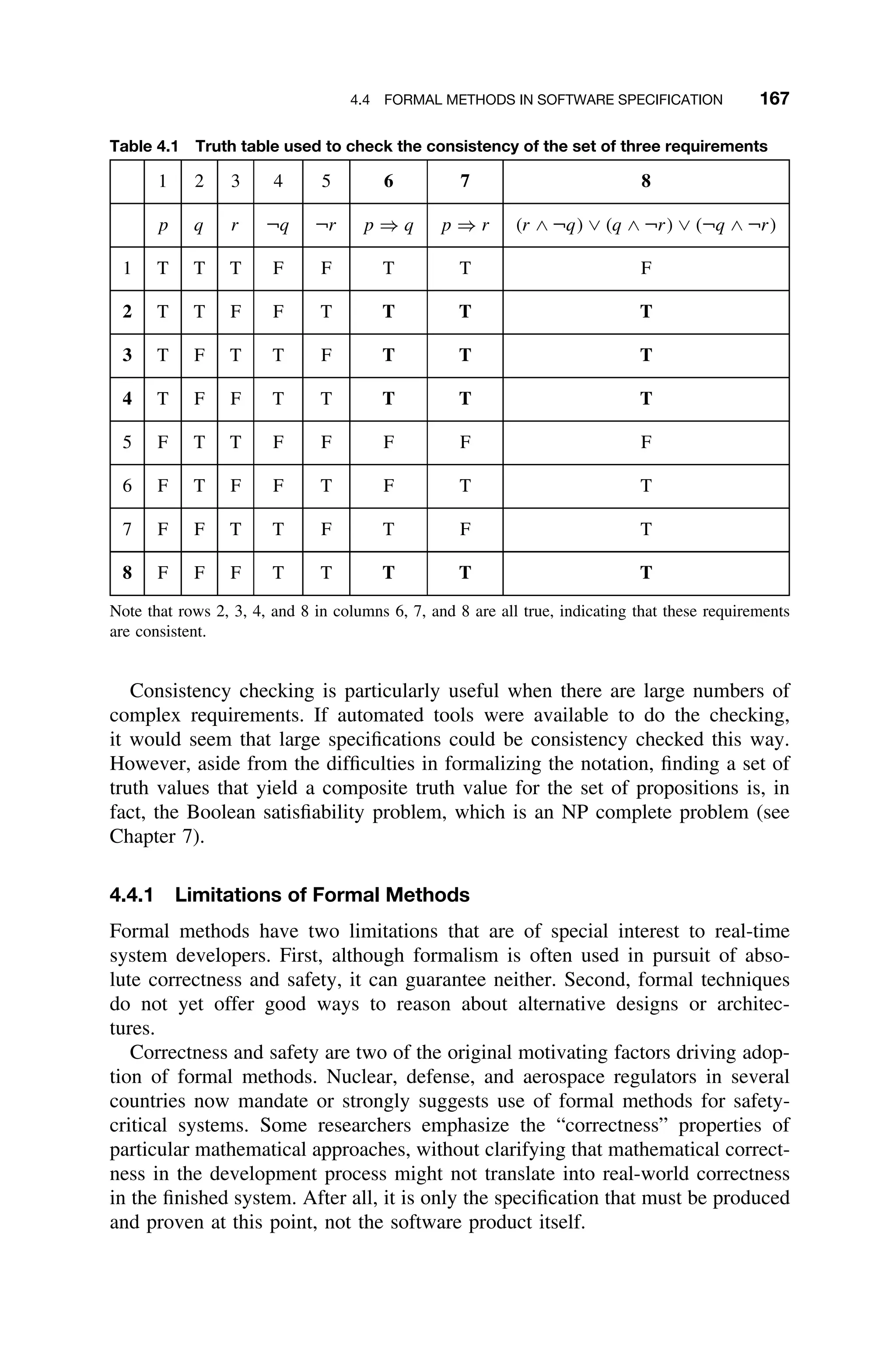
![168 4 SOFTWARE REQUIREMENTS ENGINEERING
Formal software specifications must be converted to a design, and later, to a
conventional implementation language at some point. This translation process is
subject to all the potential pitfalls of any programming effort. For this reason,
testing is just as important when using formal requirement methods as when using
traditional ones, though the testing load can be reduced with formal methods.
Formal verification is also subject to many of the same limitations as traditional
testing, namely, that testing cannot prove the absence of bugs, only their presence.
Notation evolution is a slow, but ongoing process in the formal methods
community. It can take many years from when a notation is created until it
is adopted in industry. Possibly the biggest challenge in applying formal meth-
ods to real-time embedded systems is choosing an appropriate technique to match
the problem. Still, to make formal models usable by a wide spectrum of people,
requirement documents should use one or more nonmathematical notations, such
as natural language, structured text, or diagrams.
4.4.2 Z
Z (pronounced zed),1
introduced in 1982, is a formal specification language that is
based on set theory and predicate calculus. As in other algebraic approaches, the
final specification in Z is reached by a refinement process starting from the most
abstract aspects of the systems. There is a mechanism for system decomposition
known as the Schema Calculus. Using this calculus, the system specification is
decomposed in smaller pieces called schemas where both static and dynamic
aspects of system behavior are described.
The Z language does not have any support for defining timing constraints.
Therefore, several extensions for time management have emerged. For example,
Z has been integrated with real-time interval logic (RTIL), which provides for
an algebraic representation of temporal behavior.
There are other extensions of Z to accommodate the object-oriented approach,
which adds formalism for modularity and specification reuse. These extensions,
define the system state space as a composition of the state spaces of the individual
system objects. Most of these extensions also provide for information hiding,
inheritance, polymorphism, and instantiation into the Z Schema Calculus. For
example, one extension, Object-Z, includes all the aforementioned extensions and
further integrates the concepts of temporal logic, making it suitable for real-time
specification. In this language the object status is a sort of event history of object
behavior, making the language more operational than the early version of Z.
4.4.3 Finite State Machines
The finite state automaton (FSA), finite state machine (FSM), or state transition
diagram (STD) is a formal mathematical model used in the specification and
1
Z is just one of many formal specification languages. Others, such as CSP and CCS, could have
been used in this discussion instead. This is not a dismissal of these or other techniques – it is simply
a sacrifice to brevity. The reader is encouraged to refer to other texts for a more thorough treatment,
for example, [Burns90], [Shaw01].](https://image.slidesharecdn.com/epdf-230618090952-bdcb6616/75/epdf-pub_real-time-systems-design-and-analysis-pdf-191-2048.jpg)
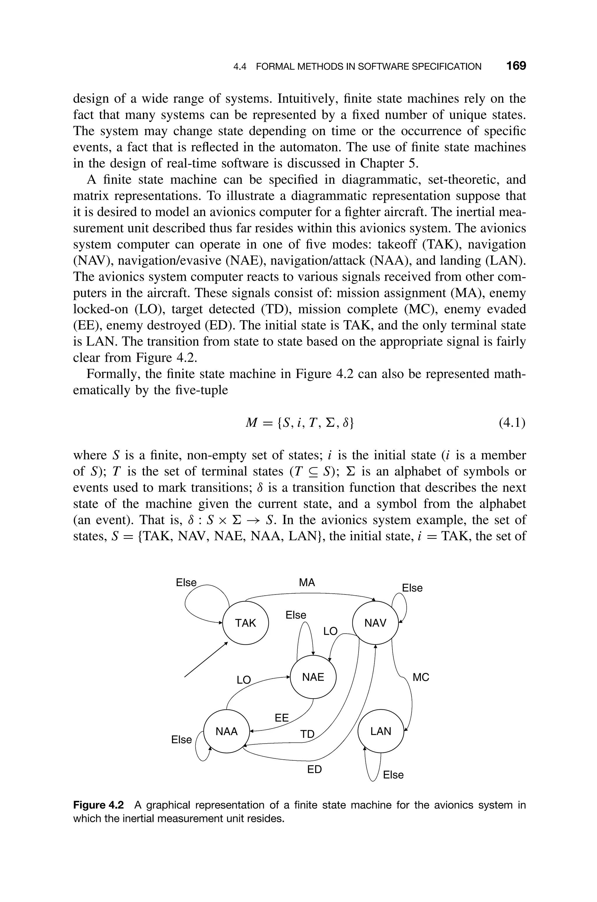
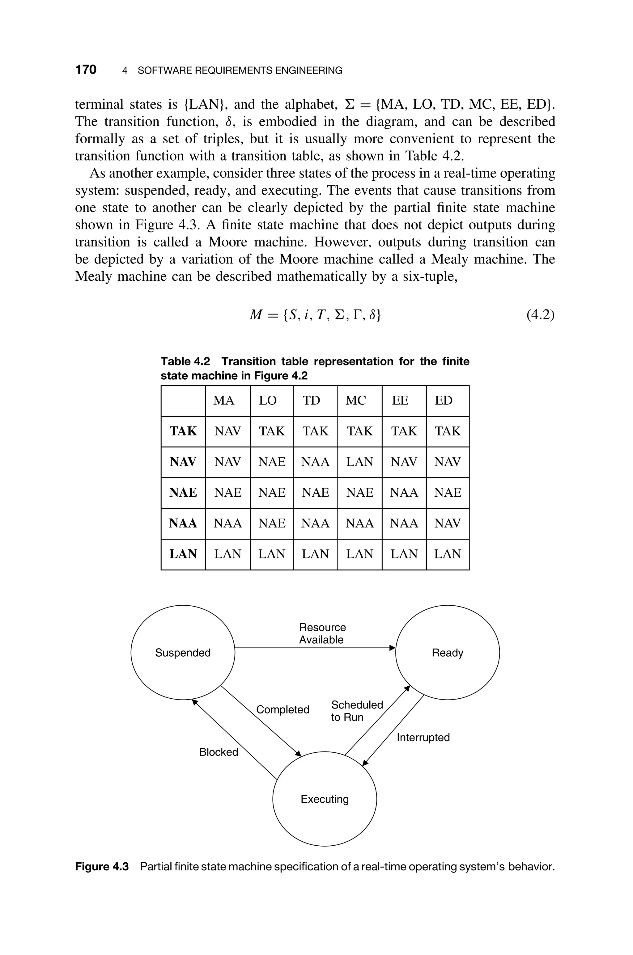
![4.4 FORMAL METHODS IN SOFTWARE SPECIFICATION 171
where the first five elements of the six-tuple are the same as for the Moore
machine and a sixth parameter, , that represents the set of outputs. The transition
function is slightly different from before in that it describes the next state of the
machine given the current state, and a symbol from the alphabet. The transition
function is then δ : S × → S × . A general Mealy machine for a system with
three states, three inputs, and three outputs is shown in Figure 4.4. The transition
matrix for the FSM shown in Figure 4.4 is shown in Table 4.3.
Finite state machines are easy to develop, and code can be easily generated
using tables to represent the transitions between states. They are also unambigu-
ous, since they can be represented with a formal mathematical description. In
addition, concurrency can be depicted by using multiple machines.
Because mathematical techniques for reducing the number of states exist, pro-
grams based on FSMs can be formally optimized. A rich theory surrounds finite
state machines, and this can be exploited in the development of system specifi-
cations. On the other hand, the major disadvantage of FSMs is that the internal
aspects, or “insideness” of modules cannot be depicted. That is, there is no way to
indicate how functions can be broken down into subfunctions. In addition, inter-
task communication for multiple FSMs is difficult to depict. Finally, depending
on the system and alphabet used, the number of states can grow very large. Both
of these problems, however, can be overcome through the use of statecharts.
S1 S2
S3
e2/o2 e2/o2
e3/o3
e3/o3
e1/o1
e1/o1
e1/o1
e2/o2
e3/o3
Figure 4.4 A generic Mealy machine for a three-state system with events e1, e2, e3 and
outputs o1, o2, o3 [Laplante03c].
Table 4.3 Transition matrix for FSM in Figure 4.4
S1 S2 S3
e1 S1/S1 S1/S1 S1/S1
e2 S2/O2 S2/O2 S2/O2
e3 S3/O3 S3/O3 S3/O3](https://image.slidesharecdn.com/epdf-230618090952-bdcb6616/75/epdf-pub_real-time-systems-design-and-analysis-pdf-194-2048.jpg)
![172 4 SOFTWARE REQUIREMENTS ENGINEERING
4.4.4 Statecharts
Statecharts combine finite state machines with data flow diagrams and a feature
called broadcast communication in a way that can depict synchronous and
asynchronous operations. Statecharts can be described succinctly as statecharts =
FSM + depth + orthogonality + broadcast communication (Figure 4.5). Here,
FSM is a finite state machine, depth represents levels of detail, orthogonality
represents the existence of separate tasks, and broadcast communication is a
method for allowing different orthogonal processes to react to the same event.
The statechart resembles a finite state machine where each state can contain its
own FSM that describes its behavior. The various components of the statechart
are depicted as follows:
1. The FSM is represented in the usual way, with capital letters or descriptive
phrases used to label the states.
2. Depth is represented by the insideness of states.
3. Broadcast communications are represented by labeled arrows, in the same
way as FSMs.
4. Orthogonality is represented by dashed lines separating states.
5. Symbols a, b, . . . , z represent events that trigger transitions, in the same
way that transitions are represented in FSMs.
6. Small letters within parentheses represent conditions that must be true for
the transitions to occur.
A significant feature of statecharts is the encouragement of top-down design
of a module. For example, for any module (represented like a state in an FSM),
increasing detail is depicted as states internal to it. In Figure 4.6 the system is
composed of states A and B. Each of these in turn can be decomposed into states
A1, A2, and B1 and B2, respectively, which might represent program modules.
Those states can also be decomposed, and so forth. To the software designer,
each nested substate within a state represents a procedure within a procedure.
Orthogonality depicts concurrency in the system for processes that run in iso-
lation, called AND states. Orthogonality is represented by dividing the orthogonal
components by dashed lines. For example, if state Y consists of AND components
A B
X | x/y |x(e1,...,en) | x(e1,...,en)/y
Figure 4.5 Statechart format where A and B are states, x is an event that causes the transition
marked by the arrow, y is an optional event triggered by x, and e1, . . . , en are conditions
qualifying the event [Laplante03c].](https://image.slidesharecdn.com/epdf-230618090952-bdcb6616/75/epdf-pub_real-time-systems-design-and-analysis-pdf-195-2048.jpg)
![4.4 FORMAL METHODS IN SOFTWARE SPECIFICATION 173
e/f
A
B
A1
A2
a1 a2
B1
B2
b1 b2
Figure 4.6 A statechart depicting insideness [Laplante03c].
A and D, Y is called the orthogonal product of A and D. If Y is entered from the
outside (without any additional information), then the states A and D are entered
simultaneously. Communication between the AND states can be achieved through
global memory, whereas synchronization can be achieved through a capability
of statecharts called broadcast communication.
Broadcast communication is depicted by the transition of orthogonal states
based on the same event. For example, if the inertial measurement system switches
from standby to ready mode, an event indicated by an interrupt can cause a state
change in several processes. Another unique aspect of broadcast communication
is the concept of the chain reaction; that is, events triggering other events. The
implementation follows from the fact that statecharts can be viewed as an exten-
sion of Mealy machines, and output events can be attached to the triggering
event. In contrast with the Mealy machine, however, the output is not seen by
the outside world; instead it affects the behavior of an orthogonal component.
For example, in Figure 4.7 suppose there exists a transition labeled e/f , and if
event e occurs then event f is immediately activated. Event f could, in turn,
trigger a transaction such as f/g. The length of a chain reaction is the number
of transitions triggered by the first event. Chain reactions are assumed to occur
instantaneously. In this system a chain reaction of length 2 will occur when the
A
B
e/f
C
D
f
Figure 4.7 Statechart depicting a chain reaction [Laplante03c].](https://image.slidesharecdn.com/epdf-230618090952-bdcb6616/75/epdf-pub_real-time-systems-design-and-analysis-pdf-196-2048.jpg)
![174 4 SOFTWARE REQUIREMENTS ENGINEERING
e/f transition occurs. As a further example, Figure 5 found in the Case Study
in Section 4.10 illustrates a statechart corresponding to the traffic intersection
control system.
Statecharts are excellent for representing embedded systems because they can
easily depict concurrency while preserving modularity. In addition, the concept
of broadcast communication allows for easy intertask.
In summary, the statechart combines the best of data flow diagrams and finite
state machines. Finally, commercial products allow an engineer to graphically
design a real-time system using statecharts, perform detailed simulation analysis,
and generate Ada or C code. Furthermore Statecharts can be used in conjunction
with both structured and object-oriented analysis.
4.4.5 Petri Nets
Petri nets are another formal method used to specify the operations to be per-
formed in a multiprocessing or multitasking environment. While they have a
rigorous foundation, they can also be described graphically. A series of circular
bubbles called “places” are used to represent data stores or processes. Rectangular
boxes are used to represent transitions or operations. The processes and transi-
tions are labeled with a data count and transition function, respectively, and are
connected by unidirectional arcs.
Table 4.4 Transition table for Petri net
shown in Figure 4.8 [Laplante03c]
P1 P2
Before firing 1 0
After firing 0 1
Before firing
P1 P2
P2
T1
T1
P1
After firing
Figure 4.8 Petri net firing rule [Laplante03c].](https://image.slidesharecdn.com/epdf-230618090952-bdcb6616/75/epdf-pub_real-time-systems-design-and-analysis-pdf-197-2048.jpg)
![4.4 FORMAL METHODS IN SOFTWARE SPECIFICATION 175
The initial graph is labeled with markings given by m0, which represent the
initial data count in the process. Net markings are the result of the firing of tran-
sitions. A transition, t, fires if it has as many inputs as required for output. In
Petri nets, the graph topology does not change over time; only the “markings”
or contents of the places do. The system advances as transitions “fire.” To illus-
trate the notion of “firing,” consider the Petri nets given in Figure 4.7 and the
associated firing table given in Table 4.4.
As a somewhat more significant example, consider the Petri net in Figure 4.9.
Reading from left to right and top to bottom indicates the stages of firings in the
net. Table 4.5 depicts the firing table for the Petri net in Figure 4.8.
m4
m3
m2
P1
P3 P4
m0
m1
T2
T1
T3
P2
Figure 4.9 Behavior sequence of a slightly more complex Petri net [Laplante03c].
Table 4.5 Firing table for Petri net in Figure 4.9
[Laplante03c]
P1 P2 P3 P4
m0 1 1 2 0
m1 0 0 3 1
m2 0 0 2 2
m3 0 0 1 3
m4 0 0 0 4](https://image.slidesharecdn.com/epdf-230618090952-bdcb6616/75/epdf-pub_real-time-systems-design-and-analysis-pdf-198-2048.jpg)
![176 4 SOFTWARE REQUIREMENTS ENGINEERING
F1
F2
F1
F2
P1
T1
T2
P2
(a)
?
F2
F1
True
T1 F1 T2
True
F2
(b)
F1
Keep
Looping?
True
T3 (Stop looping)
T1 T3
F1
(c)
Figure 4.10 Flowchart-Petri net equivalence: (a) sequence, (b) conditional branch, (c) while
loop [Laplante03c].](https://image.slidesharecdn.com/epdf-230618090952-bdcb6616/75/epdf-pub_real-time-systems-design-and-analysis-pdf-199-2048.jpg)
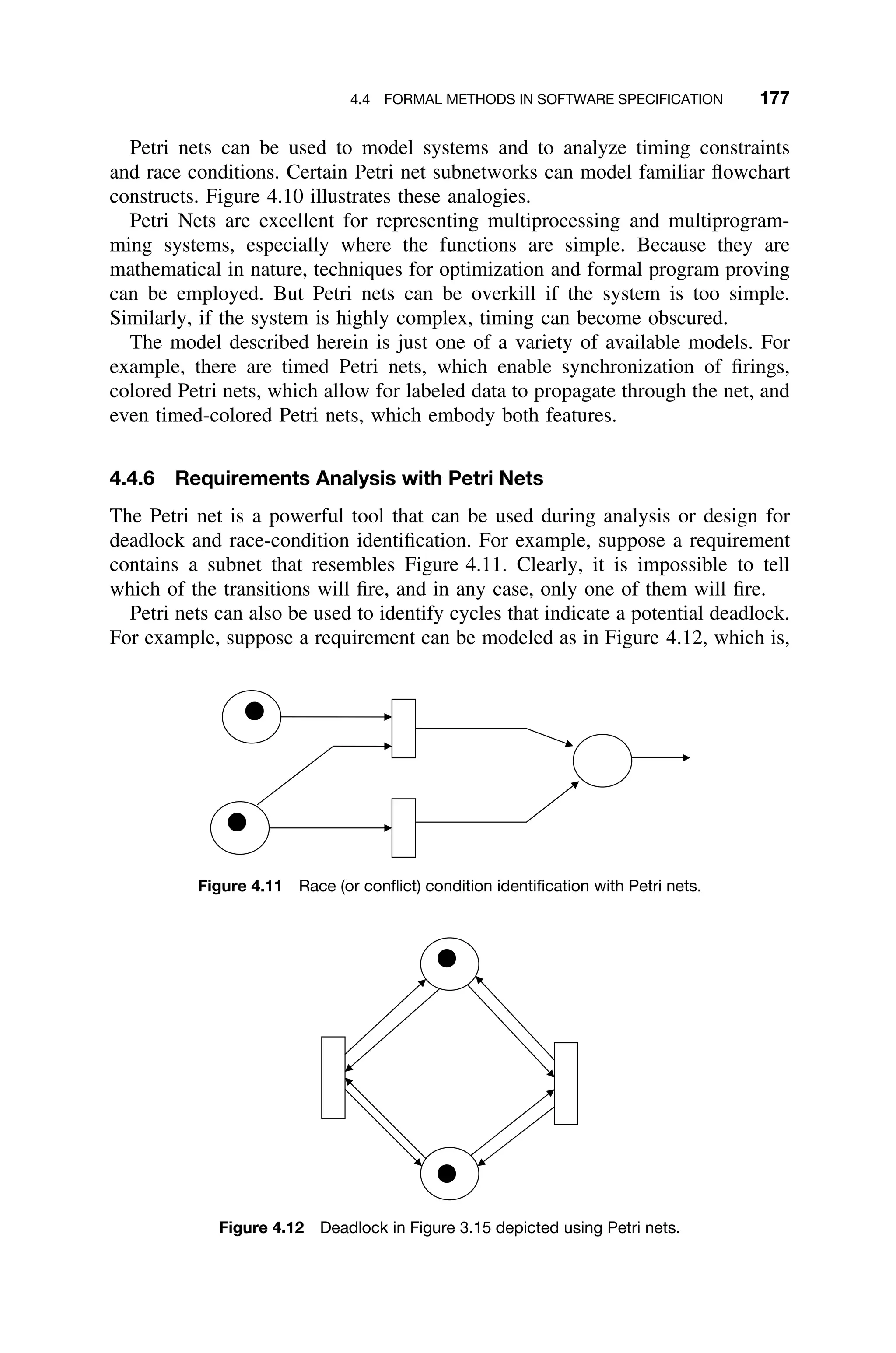
![178 4 SOFTWARE REQUIREMENTS ENGINEERING
in fact, a representation of Figure 3.15 involving two resources and two processes.
Clearly, this scenario is one of deadlock. And while it is unlikely that such an
obvious situation would be specified, Petri net analysis can be used to identify
nonobvious cycles that appear as subgraphs in more complex diagrams.
4.5 STRUCTURED ANALYSIS AND DESIGN
Methods for structured analysis and structured design (SASD) have evolved over
almost 30 years and are widely used in real-time applications, probably because
the techniques are closely associated with the programming languages with which
they co-evolved (Fortran and C) and in which many real-time applications are
written. Structured methods appear in many forms, but the de facto standard is
Yourdon’s Modern Structured Analysis [Yourdon91].
Several extensions to structured analysis emerged in the 1980s to account for
system dynamics and use if for the specification of real-time systems. These
approaches include Gomaa’s DARTS (design approach for real-time systems)
[Gomaa00]. Ward and Mellor extended data flow diagrams by adding edges
to represent control and state machines for representing behavior. Commercial
tools that followed this approach, including Teamwork and Software Through
Pictures
, emerged in the early 1990s.
Structured analysis for real-time systems is still based on the notion of the
flow of data between successive transformations and provides little support to
identify the concurrent processes that must be implemented in a given appli-
cation. Depending upon the detail of the analysis, there is something arbitrary
in identifying the system processes. This may result in the implementation of
unnecessary processes and the possibility that a given process needs concurrency
internally [Bucci95].
Perhaps the most commonly used form of structured analysis, Yourdon’s Mod-
ern Structured Analysis uses three viewpoints to describe a system: an environ-
mental model, a behavioral model, and an implementation model. The elements
of each model are shown in Figure 4.13. The environmental model embodies the
analysis aspect of SASD and consists of a context diagram and an event list.
The purpose of the environmental model is to model the system at a high level
of abstraction. The behavioral model embodies the design aspect of SASD as a
series of data flow diagrams (DFDs), entity relationship diagrams (ERDs), pro-
cess specifications, state transition diagrams, and a data dictionary. Using various
combinations of these tools, the designer models the processes, functions, and
flows of the system in detail. Finally, in the implementation model the developer
uses a selection of structure charts, natural language, and pseudocode to describe
the system to a level that can be readily translated to code.
Structured analysis (SA) is a way to try to overcome the problems of classic
analysis using graphical tools and a top-down, functional decomposition method
to define system requirements. SA deals only with aspects of analysis that can
be structured: the functional specifications and the user interface. SA is used](https://image.slidesharecdn.com/epdf-230618090952-bdcb6616/75/epdf-pub_real-time-systems-design-and-analysis-pdf-201-2048.jpg)
![4.5 STRUCTURED ANALYSIS AND DESIGN 179
Context Diagram
Event List
Natural Language
DFD/CFD
ER Diagram
Data Dictionary
P-SPEC, C-SPEC
STD/FSM
Natural Language
Structure Charts
P-SPEC
Temporal Logic
Natural Language
Environmental
Model
Behavioral
Model
Implementation
Model
Figure 4.13 Elements of structured analysis and design [Laplante03c].
to model a system’s context (where inputs come from and where outputs go),
processes (what functions the system performs, how the functions interact, how
inputs are transformed to outputs), and content (the data the system needs to
perform its functions).
SA seeks to overcome the problems inherent in analysis through:
ž Maintainability of the target document.
ž Use of an effective method of partitioning.
ž Use of graphics.
ž Building a logical model of the system for the user before implementation.
ž Reduction of ambiguity and redundancy.
The target document for SA is called the structured specification. It consists of
a system context diagram, an integrated set of data flow diagrams showing the
decomposition and interconnectivity of components, and an event list to represent
the set of events that drive the system.
To illustrate the SA technique, consider the following simplified description of
the inertial measurement system (IMU) (Figure 4.14). Some liberties have been
taken with the notation, but this is not uncommon, as each organization tends
to have its own “house style,” that is, conventions that are dependent on tools
being used or individual preferences. From the diagram, it is easy to see the four](https://image.slidesharecdn.com/epdf-230618090952-bdcb6616/75/epdf-pub_real-time-systems-design-and-analysis-pdf-202-2048.jpg)
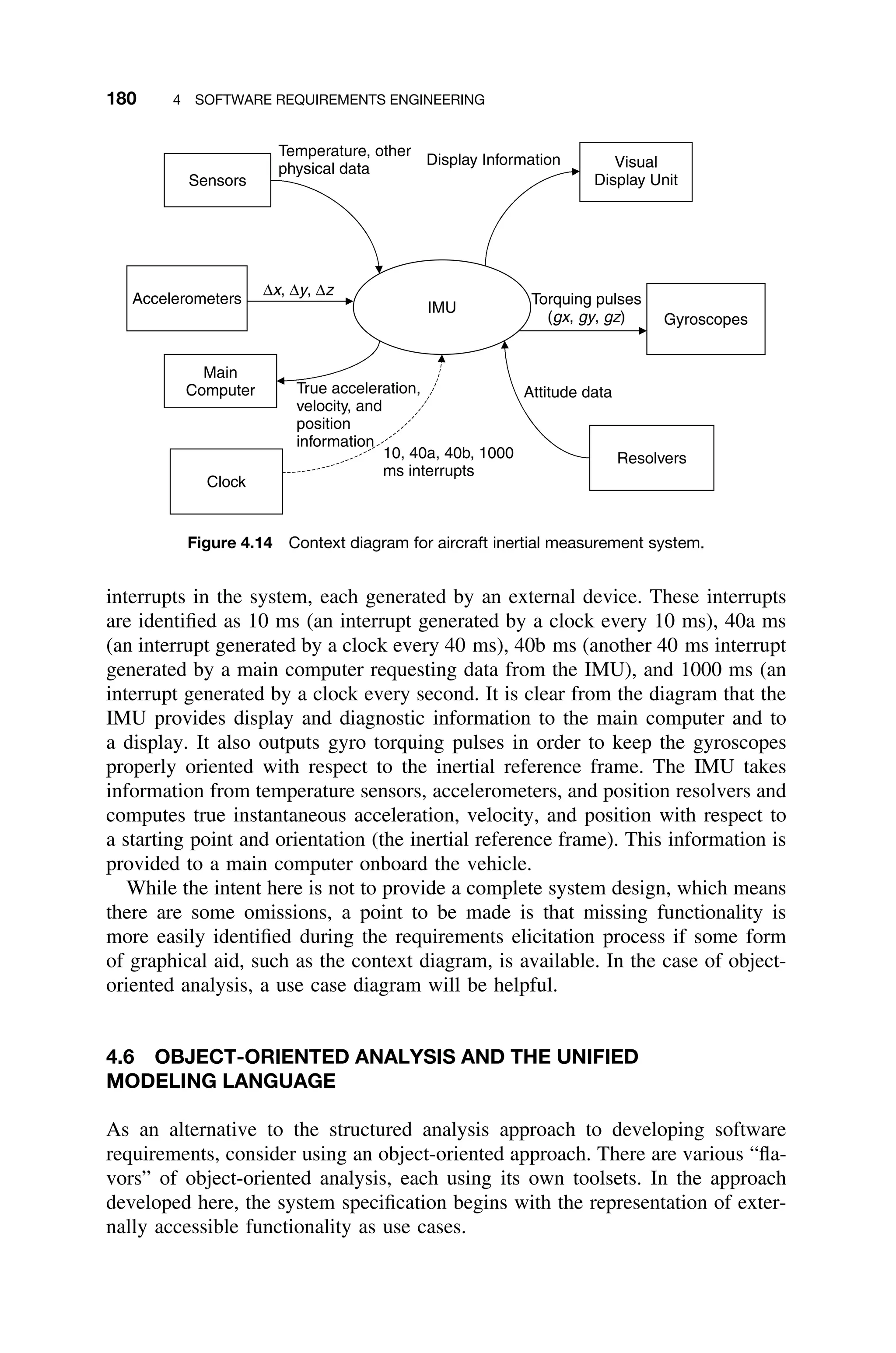
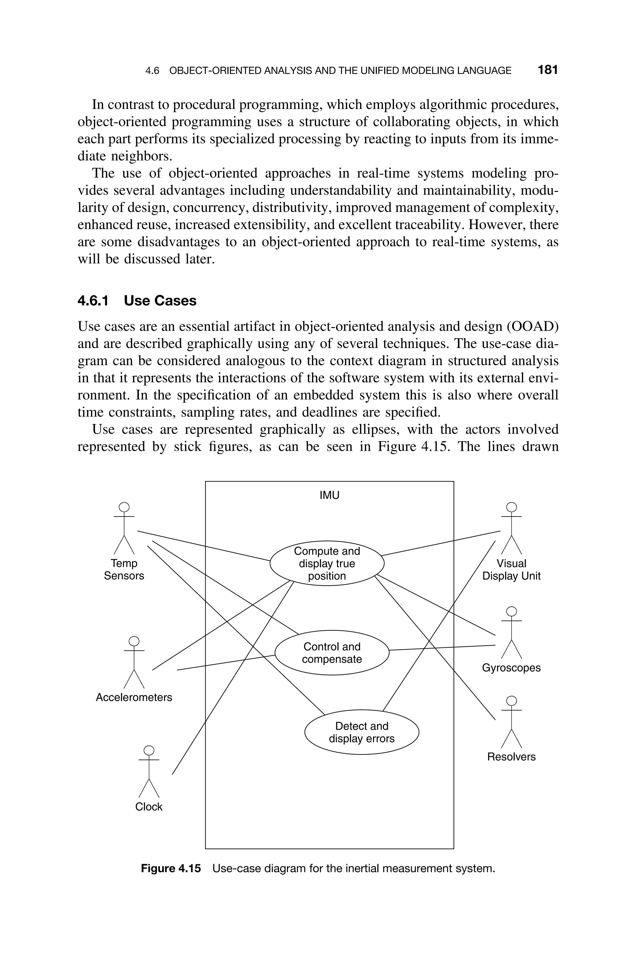
![4.7 ORGANIZING THE REQUIREMENTS DOCUMENT 183
ž Separate operational specification from descriptive behavior.
ž Use consistent levels of abstraction within models and conformance between
levels of refinement across models.
ž Model nonfunctional requirements as a part of the specification models, in
particular, timing properties.
ž Omit hardware and software assignment in the specification (another aspect
of design rather than specification).
4.7 ORGANIZING THE REQUIREMENTS DOCUMENT
There are many ways to organize the SRS, but IEEE Standard 830-1998 is the
IEEE’s Recommended Practice for Software Requirements Specifications (SRS)
[IEEE98], and provides a template of what an SRS should look like.
The SRS is described as a “binding contract among designers, programmers,
customers, and testers,” and it encompasses different design views or paradigms
for system design. The recommended design views include some combination
of decomposition, dependency, interface, and detail descriptions. Together with
boilerplate front matter, these form a standard template for software requirements
specifications, which is depicted in Figure 4.16. Sections 1 and 2 are self-evident;
they provide front matter and introductory material for the SRS. The remainder
1. Introduction
1.1 Purpose
1.2 Scope
1.3 Definitions and Acronyms
1.4 References
1.5 Overview
2. Overall Description
2.1 Product Perspective
2.2 Product Functions
2.3 User Characteristics
2.4 Constraints
2.5 Assumptions and Dependencies
3. Specific Requirements
Appendices
Index
Figure 4.16 Recommended table of contents for an SRS from IEEE Standard 830-1998
[IEEE830].](https://image.slidesharecdn.com/epdf-230618090952-bdcb6616/75/epdf-pub_real-time-systems-design-and-analysis-pdf-206-2048.jpg)
![184 4 SOFTWARE REQUIREMENTS ENGINEERING
of the SRS is devoted to the four description sections. The section headings can
be broken down further using a technique such as structured analysis.
The IEEE 830 standard provides for several alternative means to represent the
requirements specifications, aside from a function perspective. In particular, the
software requirements can be organized by
ž Functional mode (for example, “operational,” “diagnostic,” “calibration”).
ž User class (for example, “operator,” “diagnostic”).
ž Object.
ž Feature (what the system provides to the user).
ž Stimulus (e.g., sensor 1, 2, and so forth).
ž Functional hierarchy.
ž Mixed (combining two or more of the preceding).
4.8 ORGANIZING AND WRITING REQUIREMENTS
The text structure of the SRS can be depicted by the number of statement iden-
tifiers at each hierarchical level. High-level requirements rarely have numbered
statements below a depth of four (e.g., 3.2.1.5). Well-organized documents have a
pyramidal structure to the requirements. Requirements with an hourglass structure
mean too many administrative details. Diamond structured requirements indicate
subjects introduced at higher levels were addressed at different levels of detail
(Figure 4.17). Whatever approach is used in organizing the SRS, the IEEE 830
standard describes the characteristics of good requirements. That is, good require-
ments must be
1. Correct They must correctly describe the system behavior.
2. Unambiguous The requirements must be clear, not subject to different
interpretations.
3. Complete There must be no missing requirements. Ordinarily, the note
TBD [to be defined (later)] is unacceptable in a requirements document.
IEEE 830 sets out some exceptions to this rule.
1, 2, 3,4, 5, 6, 7, 8, 9, 10
1.1, 1.2, 2.1, 2.2
1.1.1, 2.1.1
1.1.1.1, 1.2.1.1
1.1.1.1.1, 1.1.1.1.2, 1.2.1.1.2
1, 2, 3
1.1, 1.2, 2.1, 2.2
1.1.1, 1.1.2, 1.2.1, 1.2.2, 2.1.1
1.1.1.1, 1.1.1.2, 1.1.2.1, 1.1.2.2, 1.2.1.1,…
1.1.1.1.1, 1.1.1.2.1, 1.1.2.2.1, 1.1.2.2.2
1.1.1.1.1.1, 1.1.2.2.1.1
1, 2, 3
1.1, 1.2, 2.1, 2.2
1.1.1, 1.1.2, 1.2.1, 1.2.2, 2.1.1
1.1.1.1, 1.1.1.2, 1.1.2.1, 1.1.2.2, 1.2.1.1,…
Figure 4.17 Triangle-, hourglass-, and diamond-shaped requirements configurations.](https://image.slidesharecdn.com/epdf-230618090952-bdcb6616/75/epdf-pub_real-time-systems-design-and-analysis-pdf-207-2048.jpg)
![4.9 REQUIREMENTS VALIDATION AND REVIEW 187
undesirable, but also can indicate ambiguity and incompleteness), flagging of key
words that may be ambiguous (e.g., “fast,” “reliable”), identification of missing
requirements (e.g., search for the phrase “to be determined”) and overly complex
sentences (which can indicate unclear requirements).
4.9.1 Requirements Validation Using Model Checking
Model checking is a formal method that can be used to perform analysis of
requirements specifications, even partial ones. The aim, however, is to find errors,
not prove correctness.
One methodology uses state machines to test for safety and liveness. The first
step involves building a state model of the system, for example, using statecharts.
Once this initial model is obtained, the state space size is estimated in order to
assess the potential for automated validation. Next, the state space is reduced
by identifying equivalence classes and by exploiting symmetries and subclasses.
Finally, a symbolic representation of the main features of the requirements are
derived. This representation represents a behavioral, temporal logic that emu-
lates the coarse-grain behavior of the system. To check for fault-tolerance, faults
are injected into the “live” model and this model is exercised to identify prob-
lems [Schneider98]. Model checking represents, in some ways, a very high-level
prototype of the requirements.
4.9.2 Automated Checking of Requirements
Automated requirements checking is used to assess certain qualities of require-
ments specifications, not to assess the correctness of the SRS (for example,
some of the challenges in automated consistency checking were discussed). One
example of such a tool is NASA’s Automated Requirements Measurement (ARM)
tool [Wilson97].
Tools, like ARM use several requirements indicators at both a coarse-grain
and fine-grain scale. Coarse-grain indicators include
ž Size of requirements
ž Text structure
ž Specification depth
ž Readability
Fine-grain measures look at the use of certain categories of words in the docu-
ments. Typical indicators are
ž Imperatives
ž Continuances
ž Directives
ž Options](https://image.slidesharecdn.com/epdf-230618090952-bdcb6616/75/epdf-pub_real-time-systems-design-and-analysis-pdf-210-2048.jpg)
![188 4 SOFTWARE REQUIREMENTS ENGINEERING
Table 4.6 Imperatives found in requirements specifications and their purpose [Wilson97]
Imperative Purpose
Shall Dictates provision of fundamental capability
Must Establishes performance requirements or constraints
Must not Establishes performance requirements or constraints
Is required to Used in specifications statements written in passive voice
Are applicable Used to include, by reference, standards or other documentation as
an addition to the requirements being specified
Responsible for Used as an imperative for systems whose architectures are already
defined
Will Generally used to cite things that the operational or development
environment are to provide to the capability being specified
Should Not recommended for use
ž Weak phrases
ž Imperatives
Imperatives are given in Table 4.6.
Continuances follow an imperative and introduce the specification of require-
ments at a lower level. Continuances include:
ž “Below”
ž “As follows”
ž “Following”
ž “Listed”
ž “In particular”
ž “Support”
Directives are words and phrases that point to illustrative information:
ž “Figure”
ž “Table”
ž “For example”
Options give the developer latitude in satisfying the specifications, and include:
ž “Can”
ž “May”
ž “Optionally”
Weak phrases, which should be avoided in SRS, include:
ž “Adequate”
ž “As a minimum”](https://image.slidesharecdn.com/epdf-230618090952-bdcb6616/75/epdf-pub_real-time-systems-design-and-analysis-pdf-211-2048.jpg)
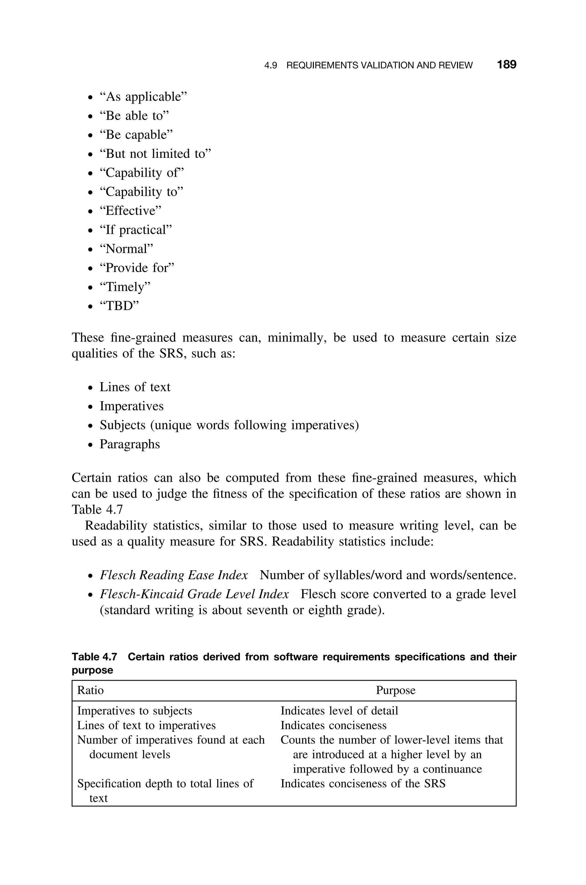
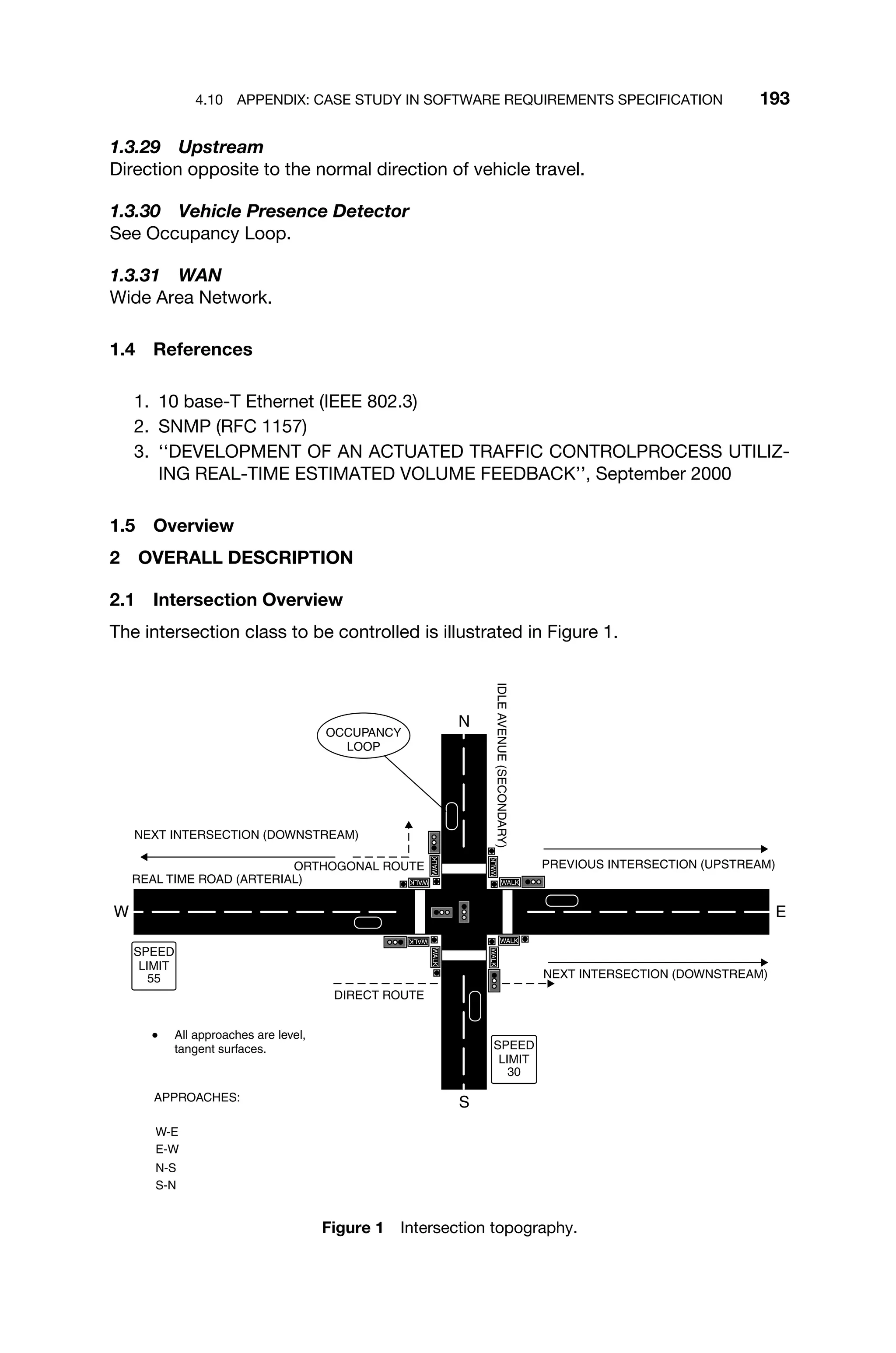
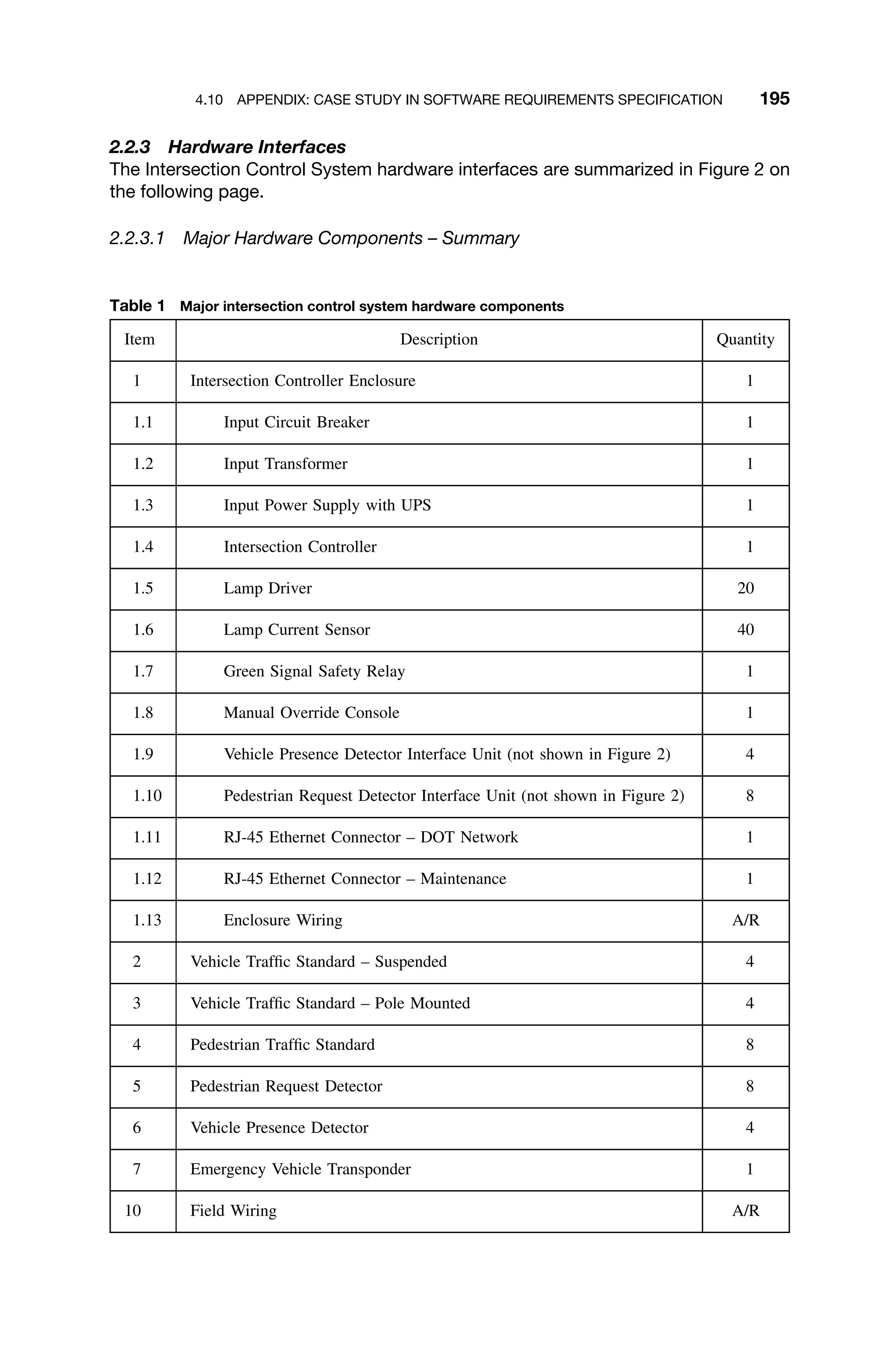
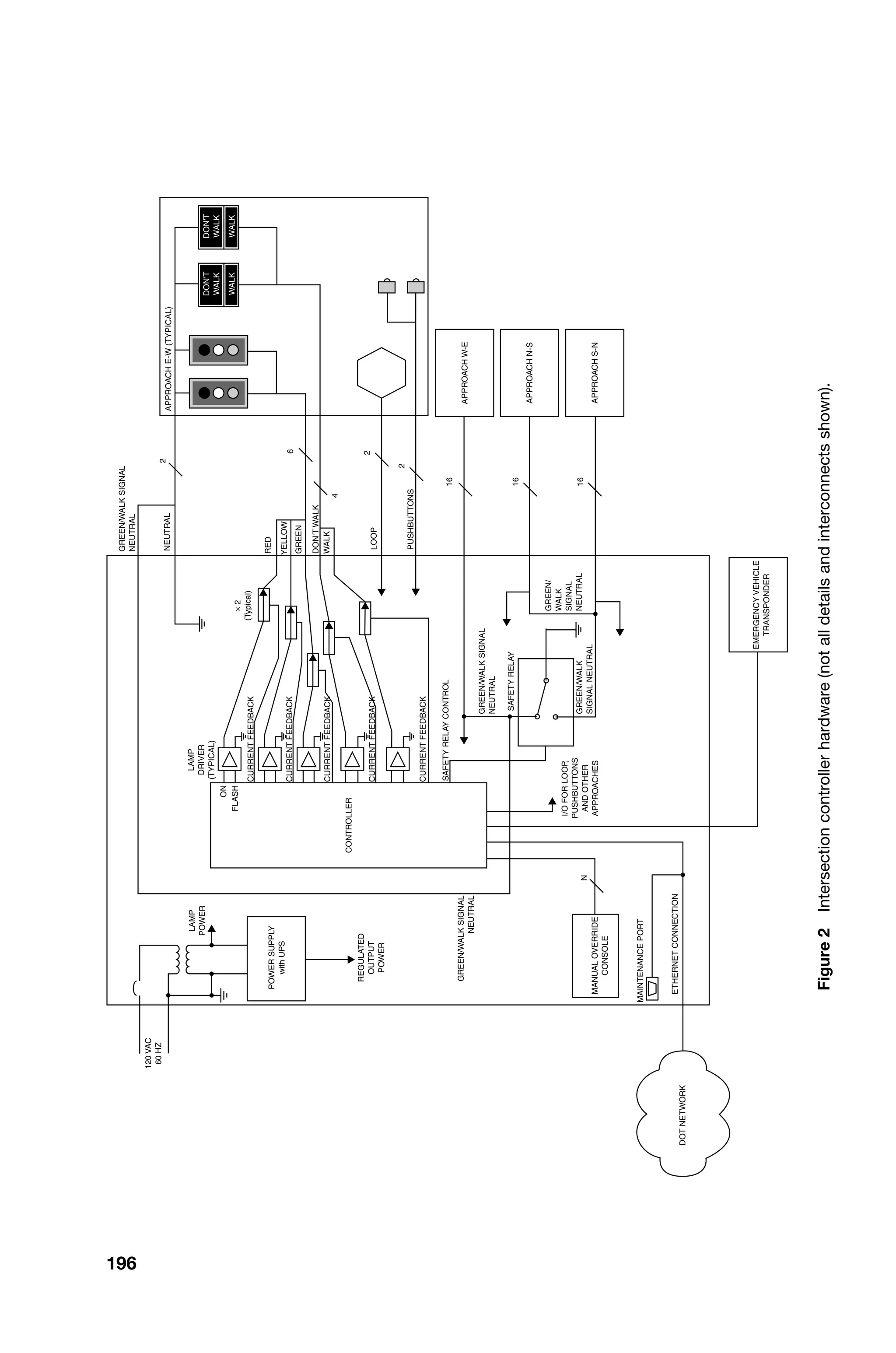

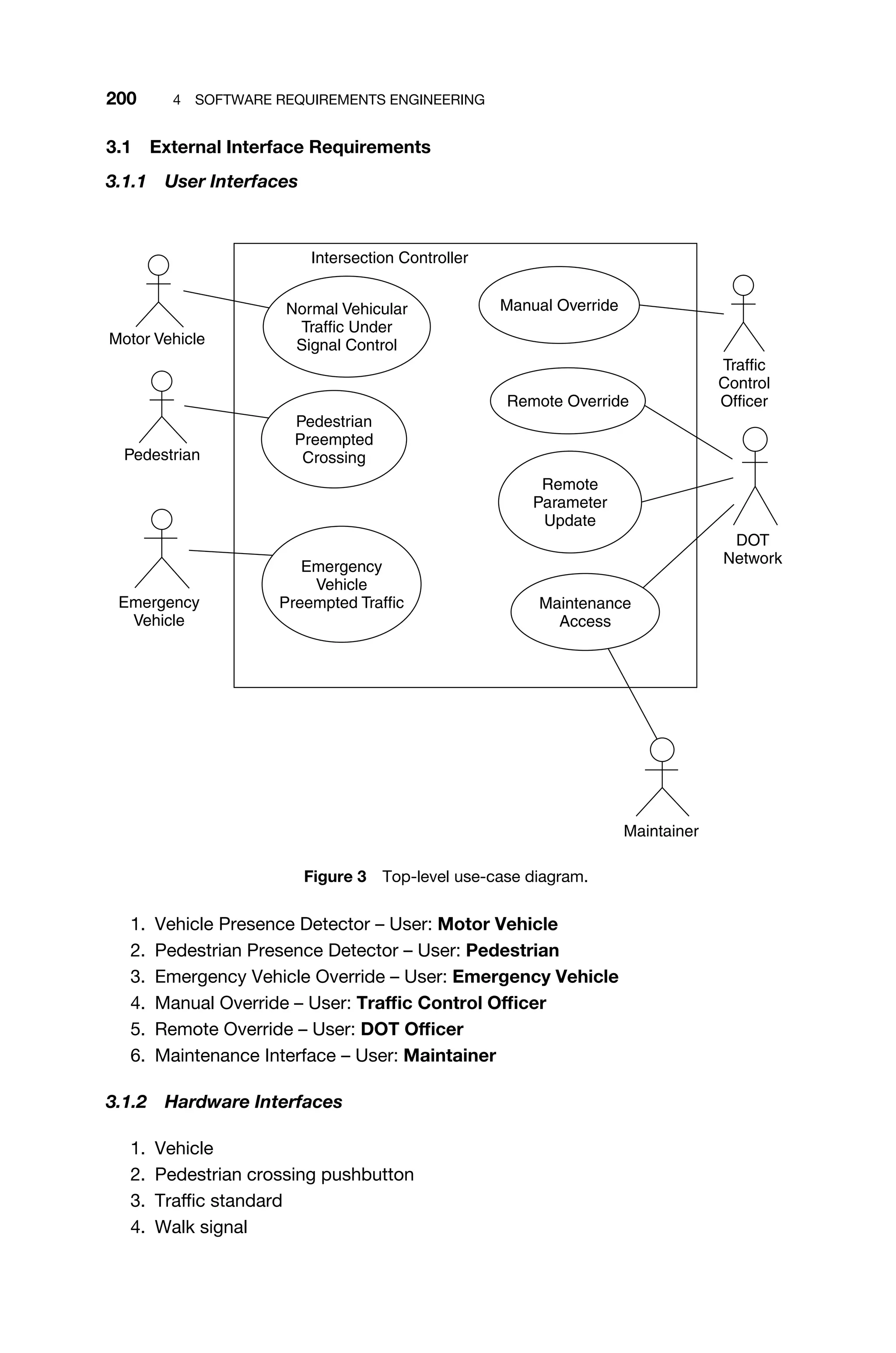
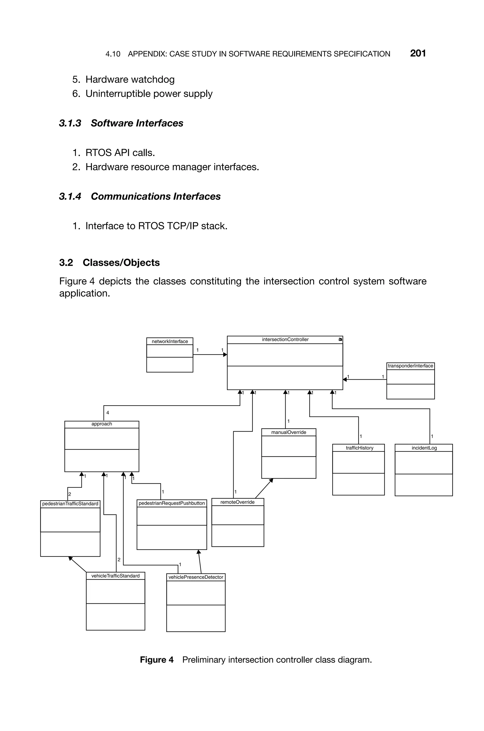
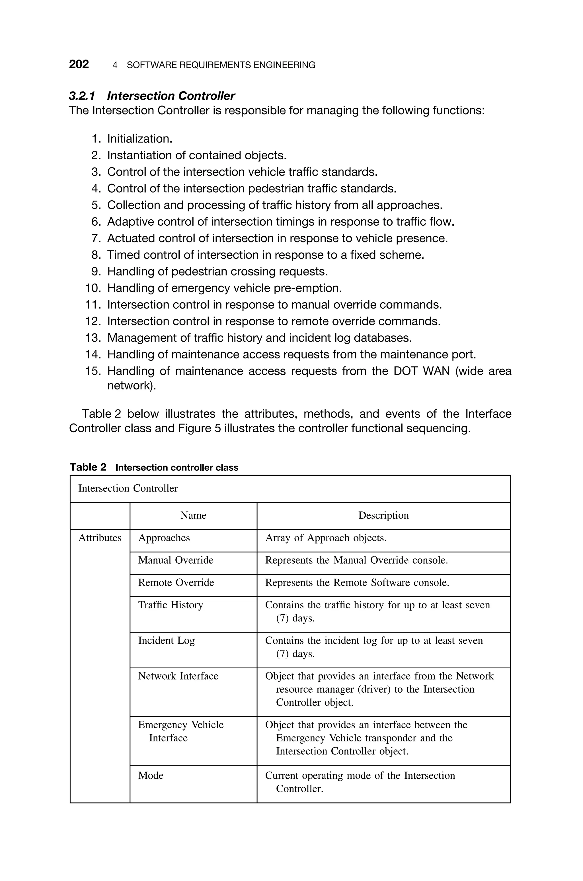
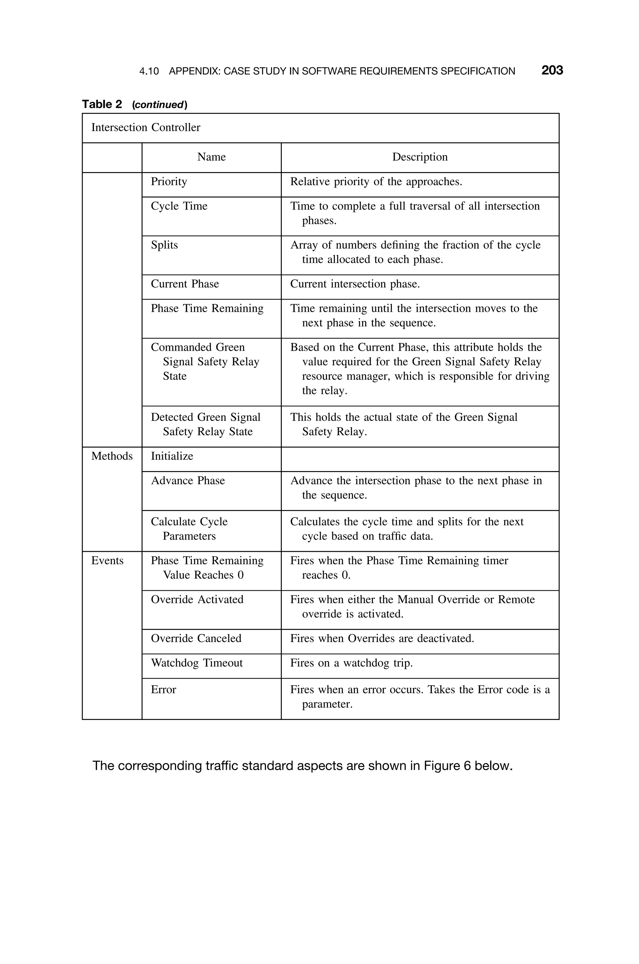
![phase_6
phase_5
init
default_2
phase_4
phase_8
phase_7
phase_1...
default_1
phase_3
default_3
phase_2
C
onTimerExpired
onTimerExpired
[priority
=
3]
onDefaultSuccess
[priority
=
2]
onTimerExpired
onTimerExpired
onInitSuccess
[priority
=
1]
onTimerExpired
onTimerExpired
onTimerExpired
onDefaultSuccess
onTimerExpired
onDefaultSuccess
Figure
5
Statechart
for
intersection
controller
phase
sequence.
204](https://image.slidesharecdn.com/epdf-230618090952-bdcb6616/75/epdf-pub_real-time-systems-design-and-analysis-pdf-227-2048.jpg)
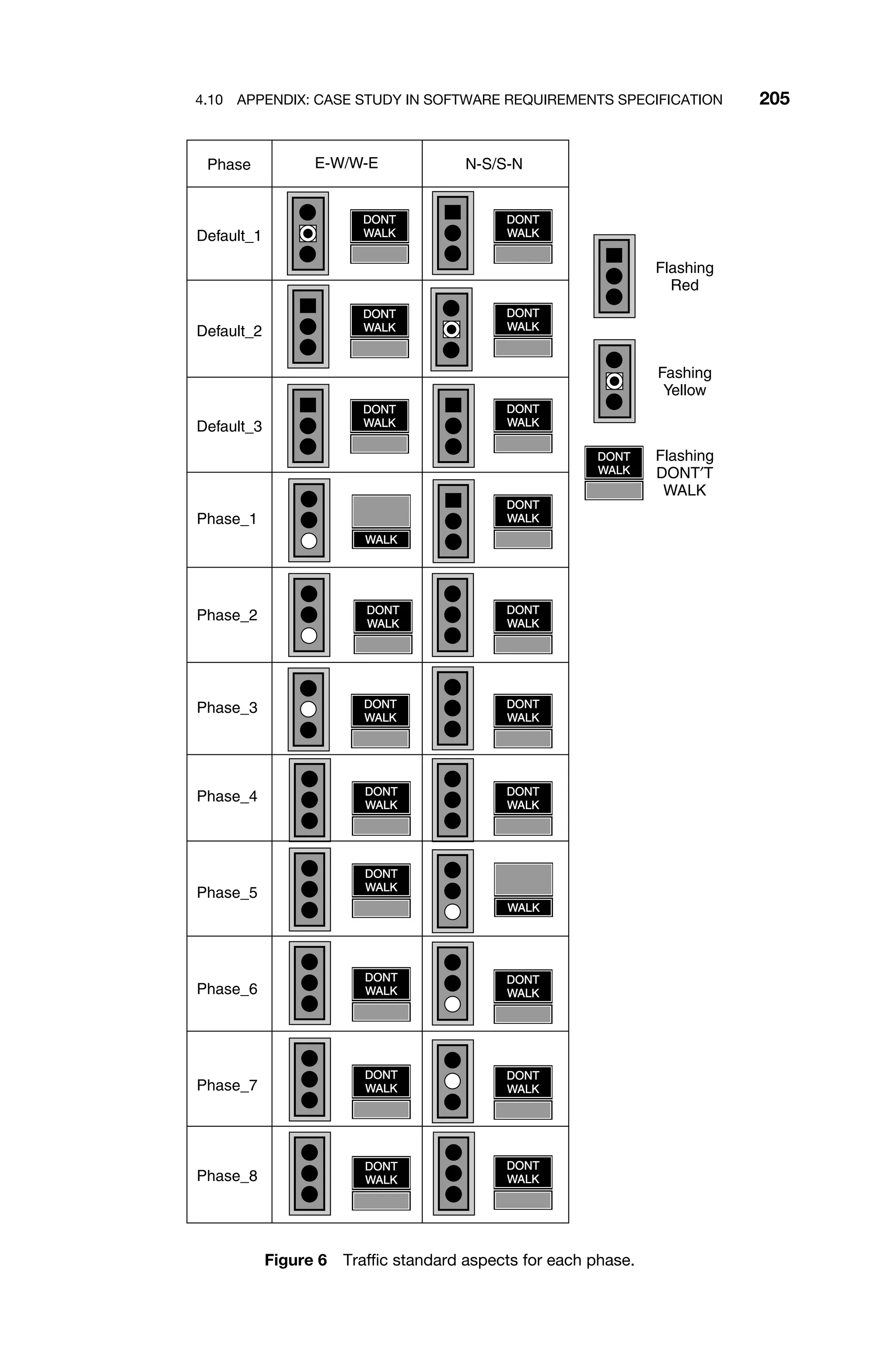
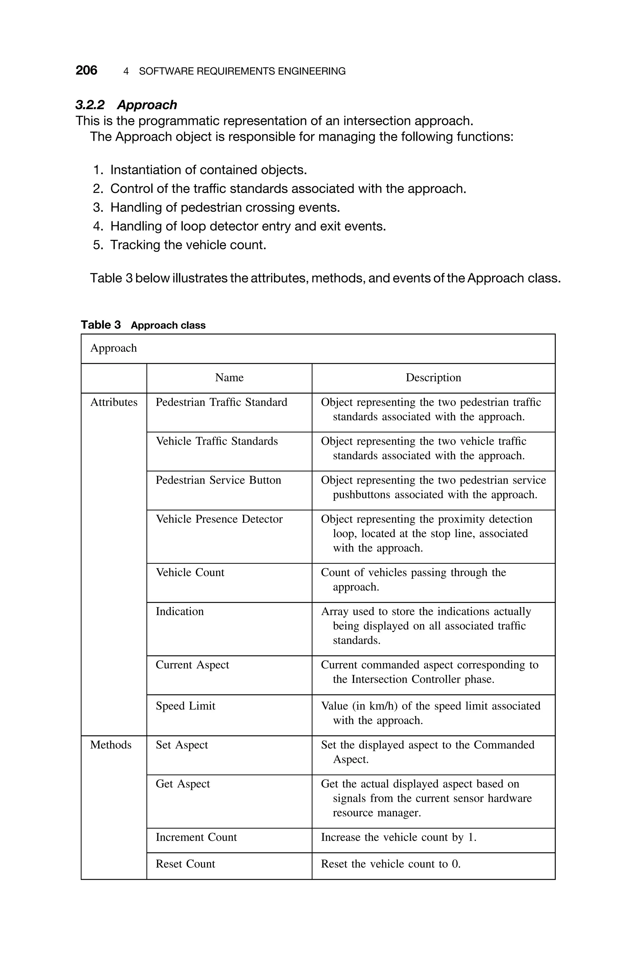
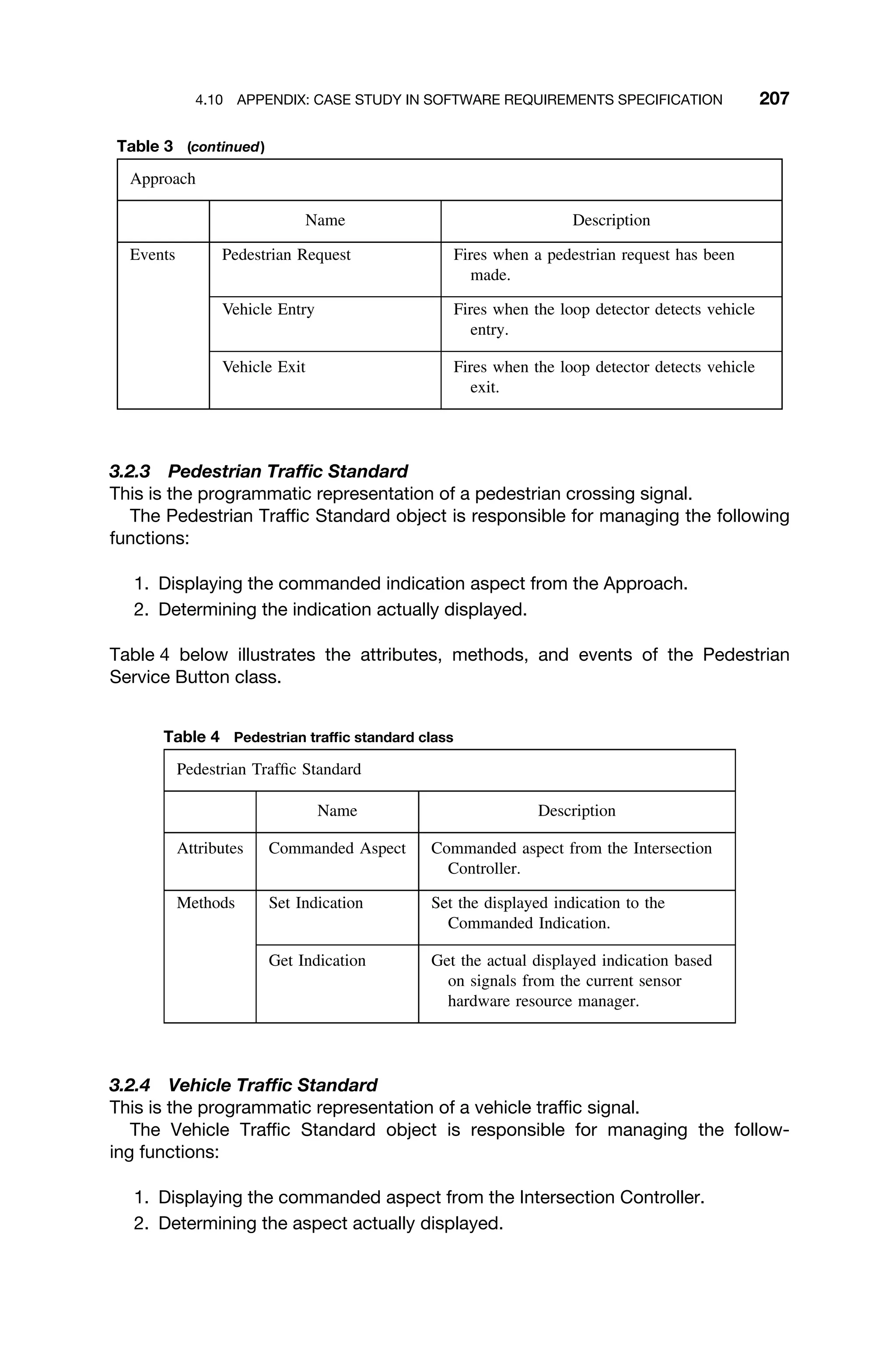
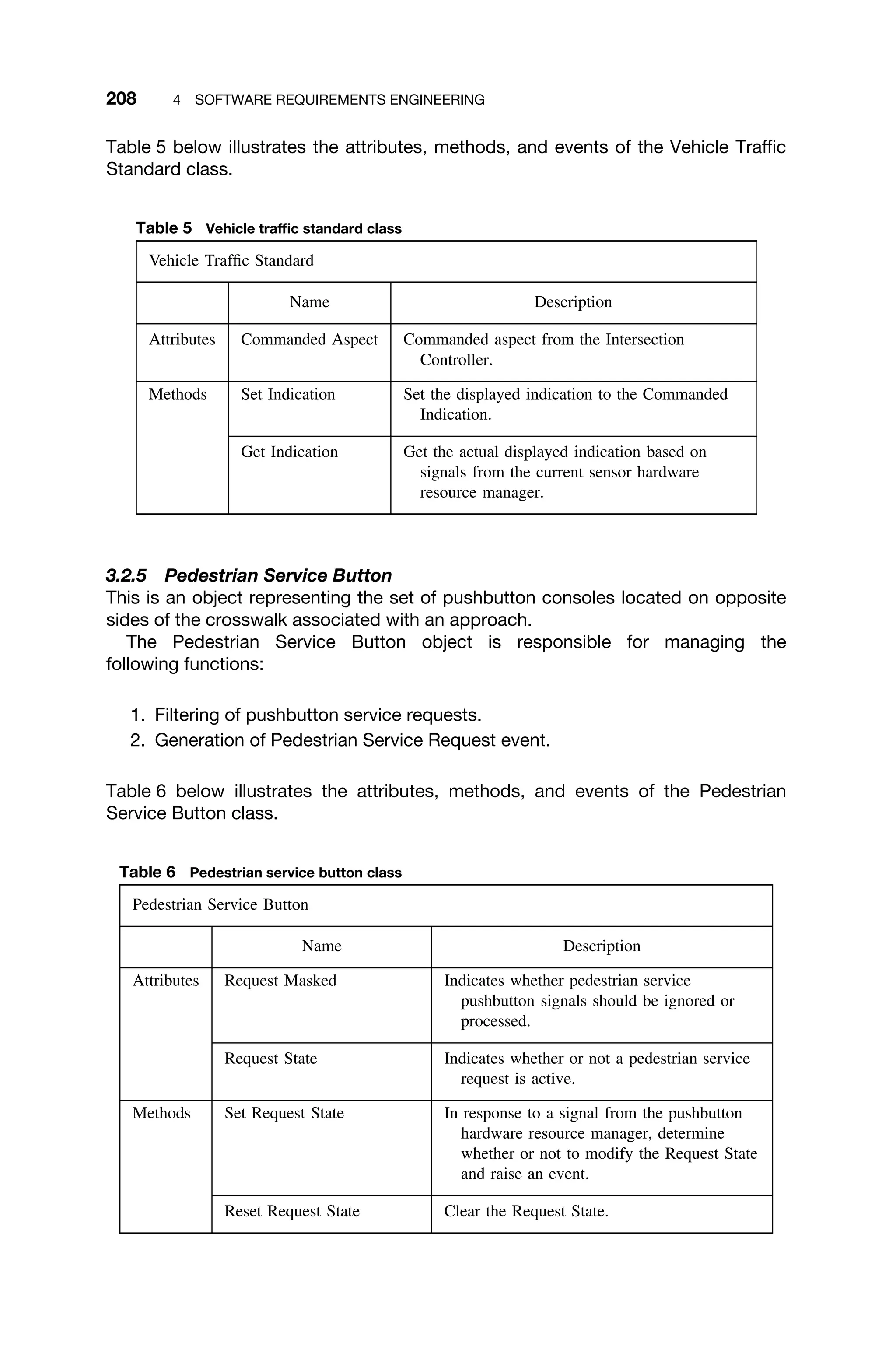
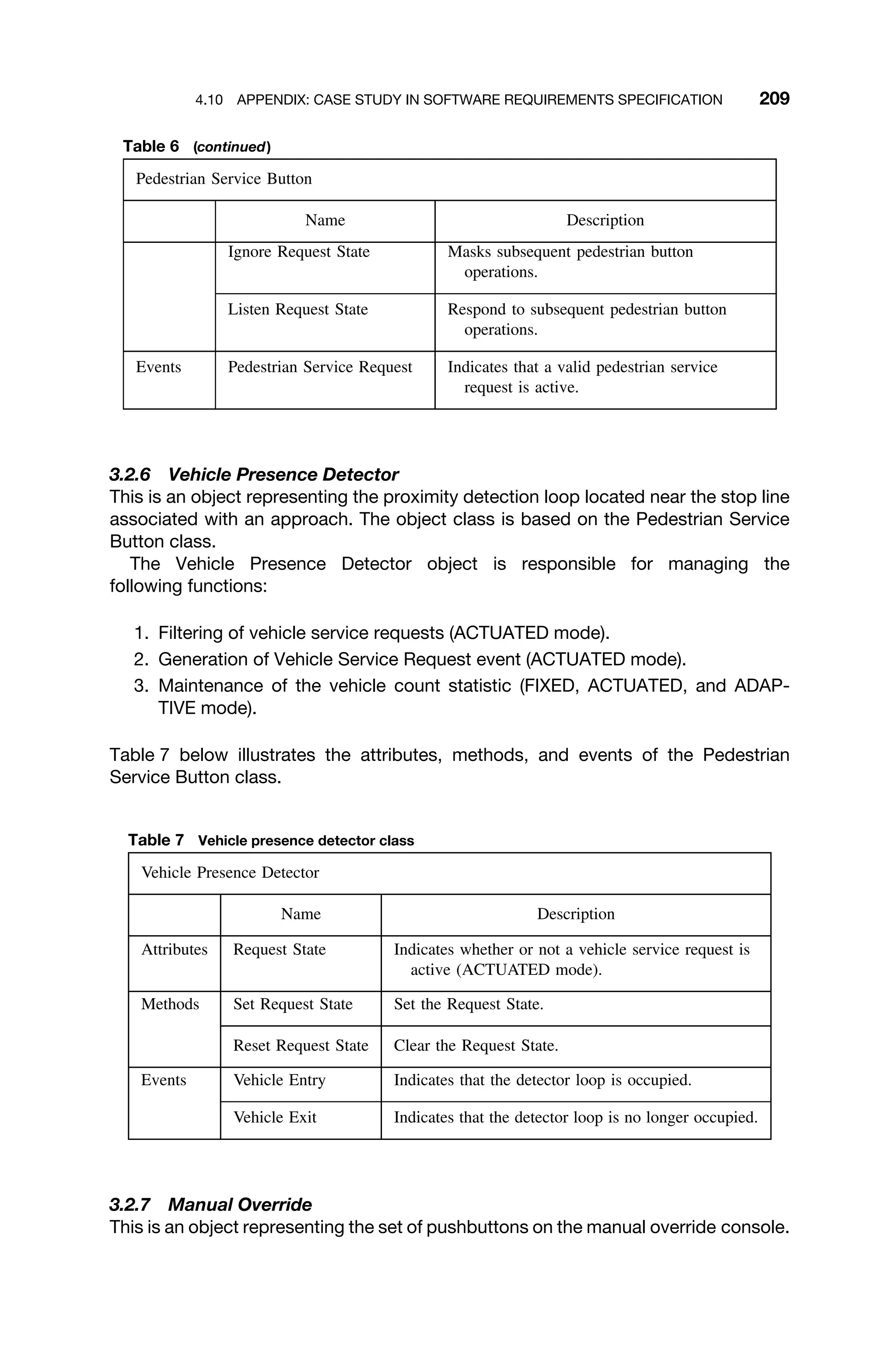
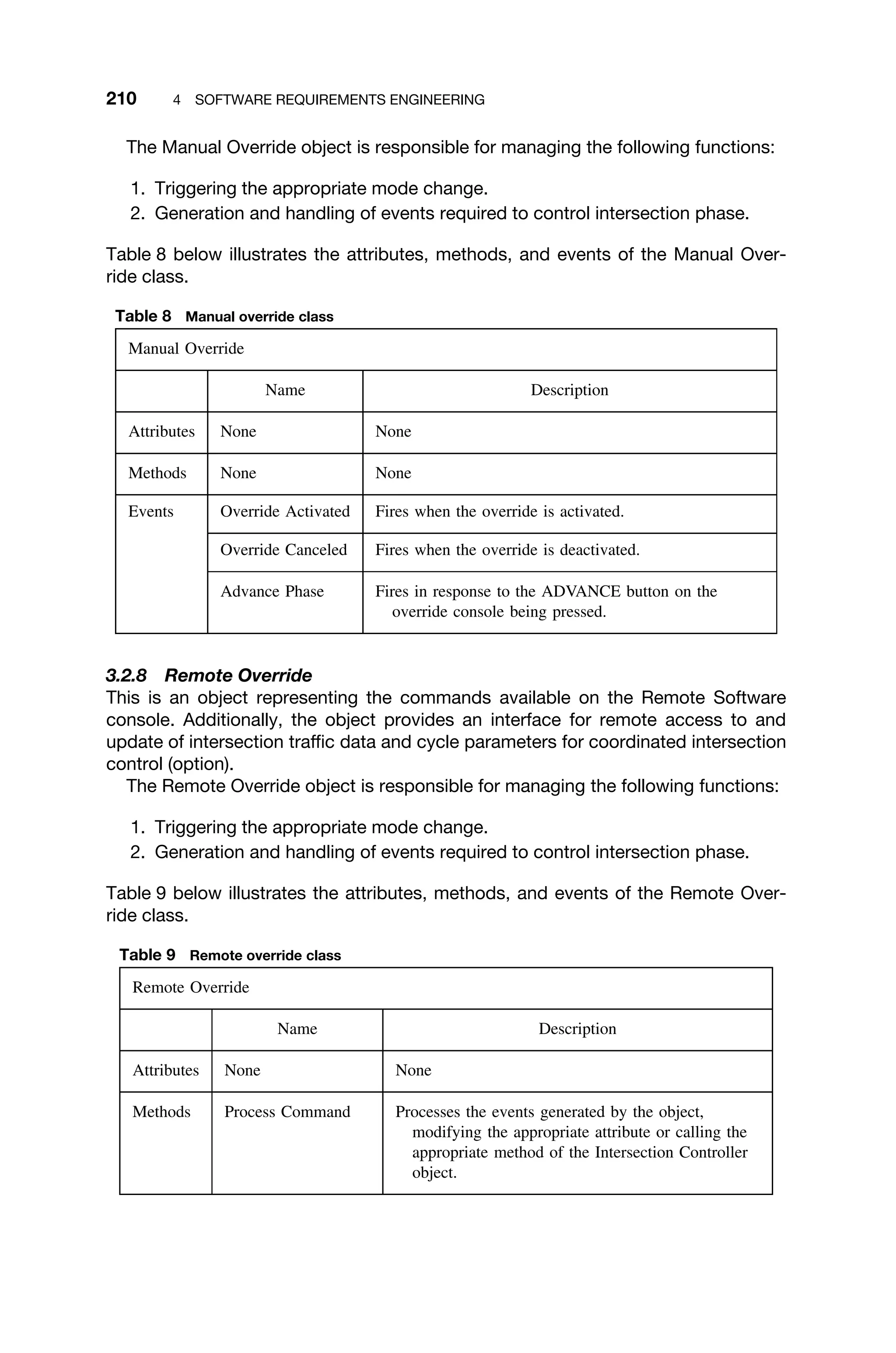
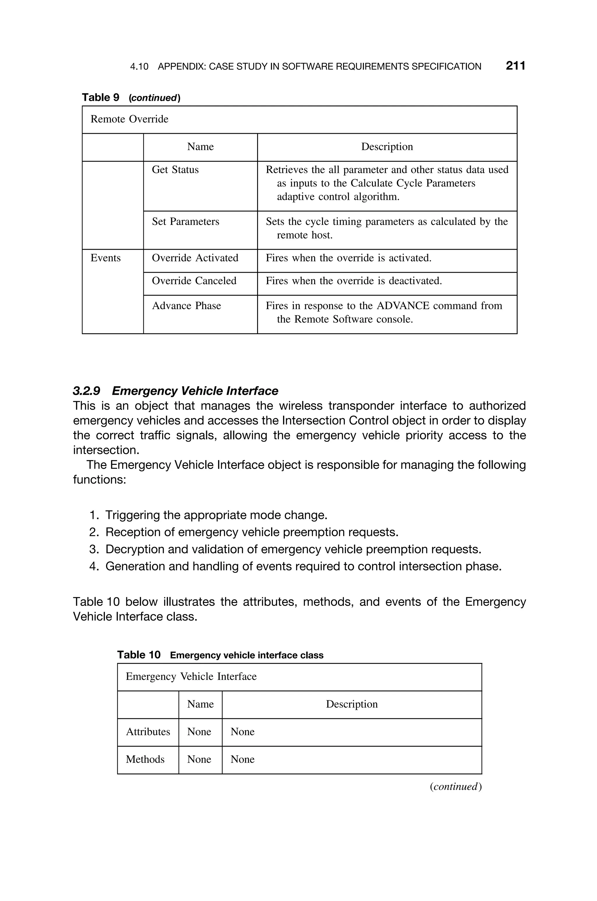

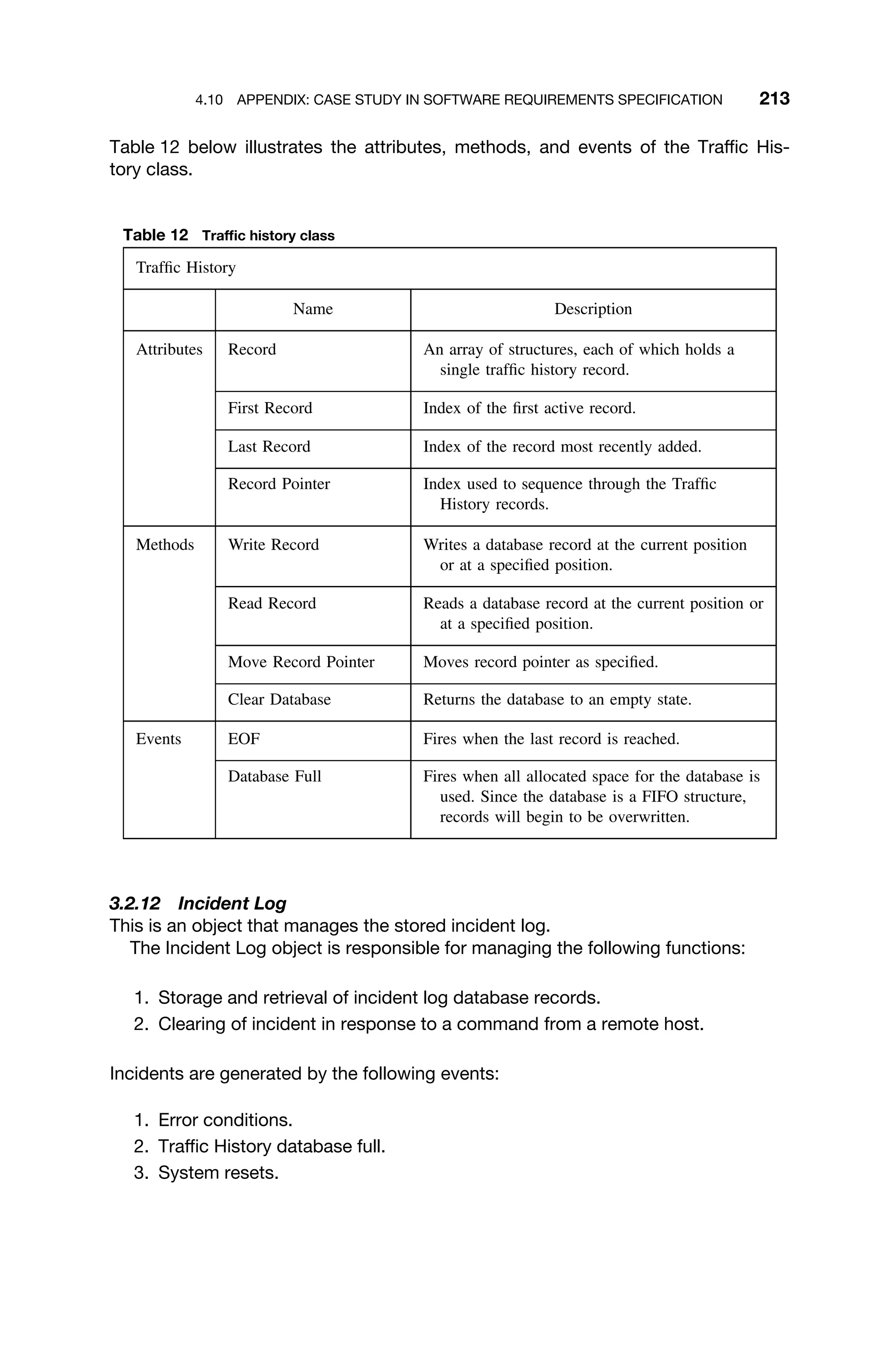
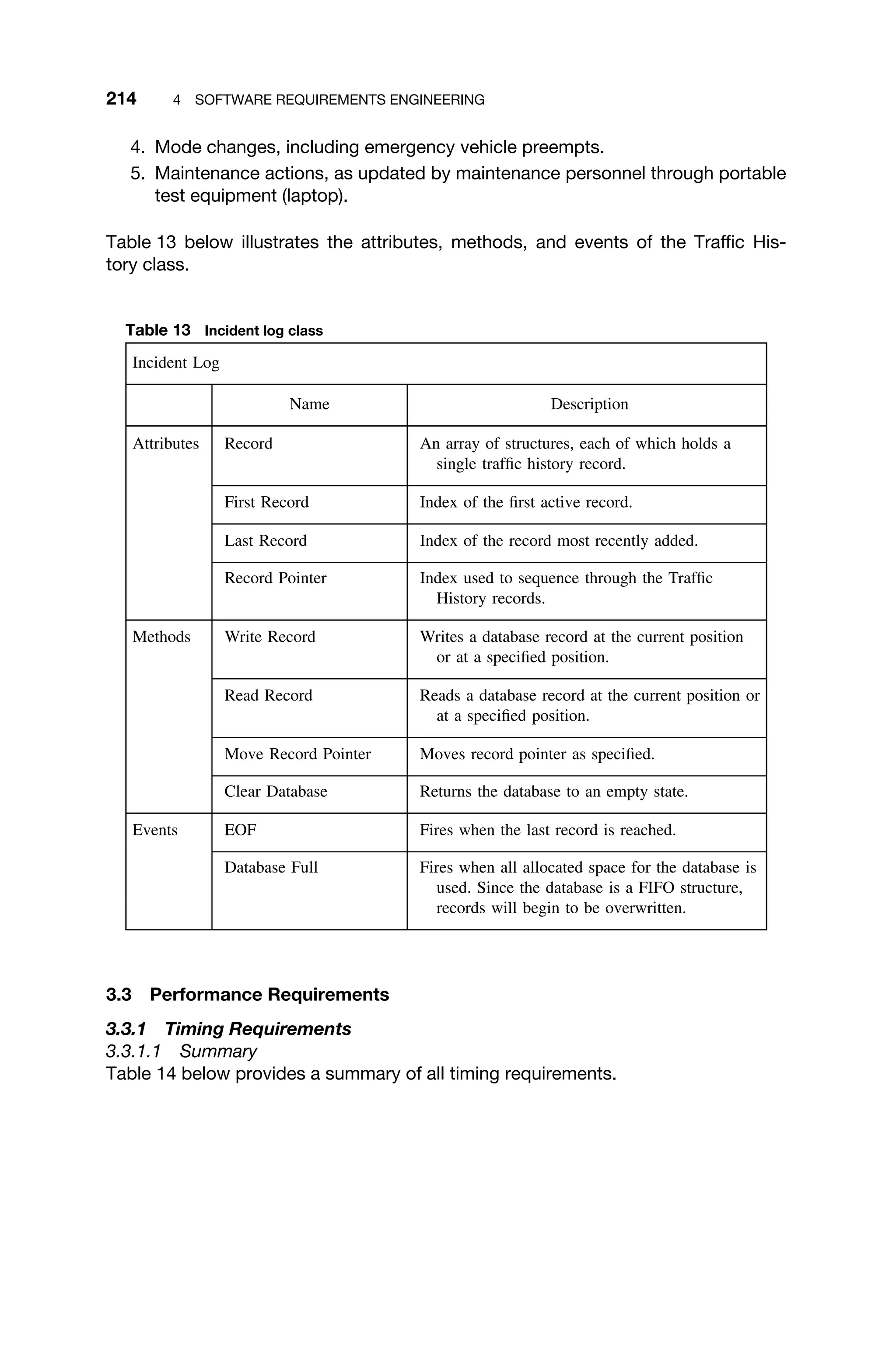
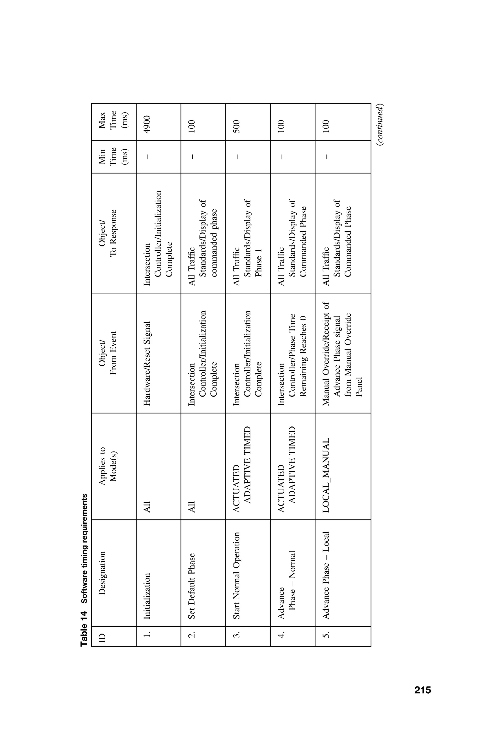
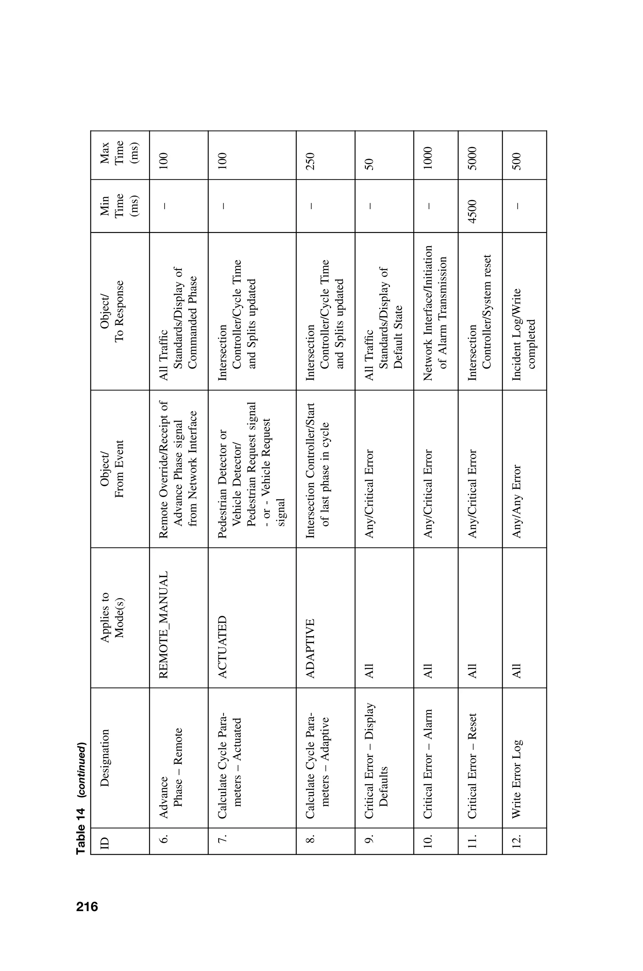
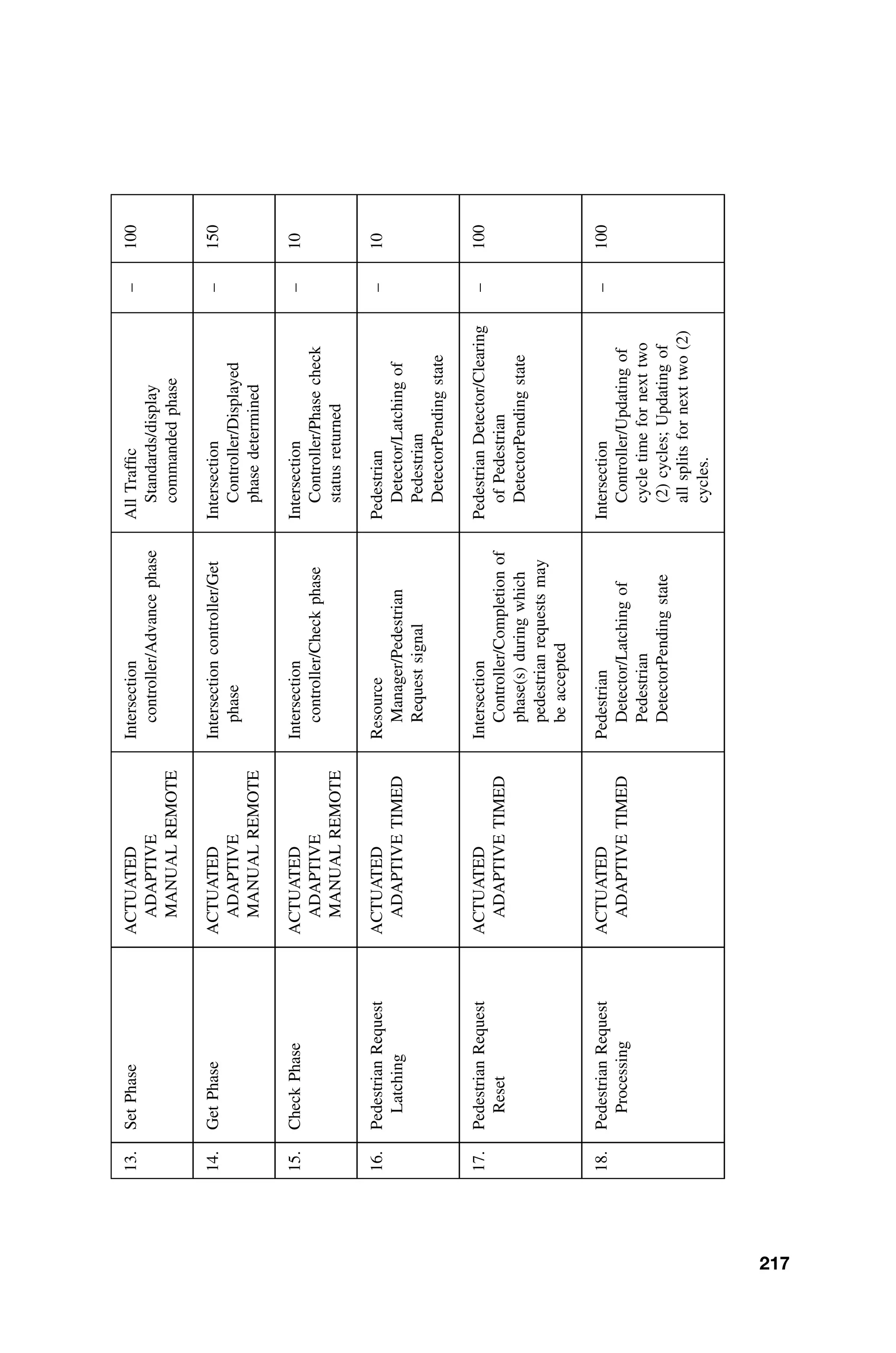
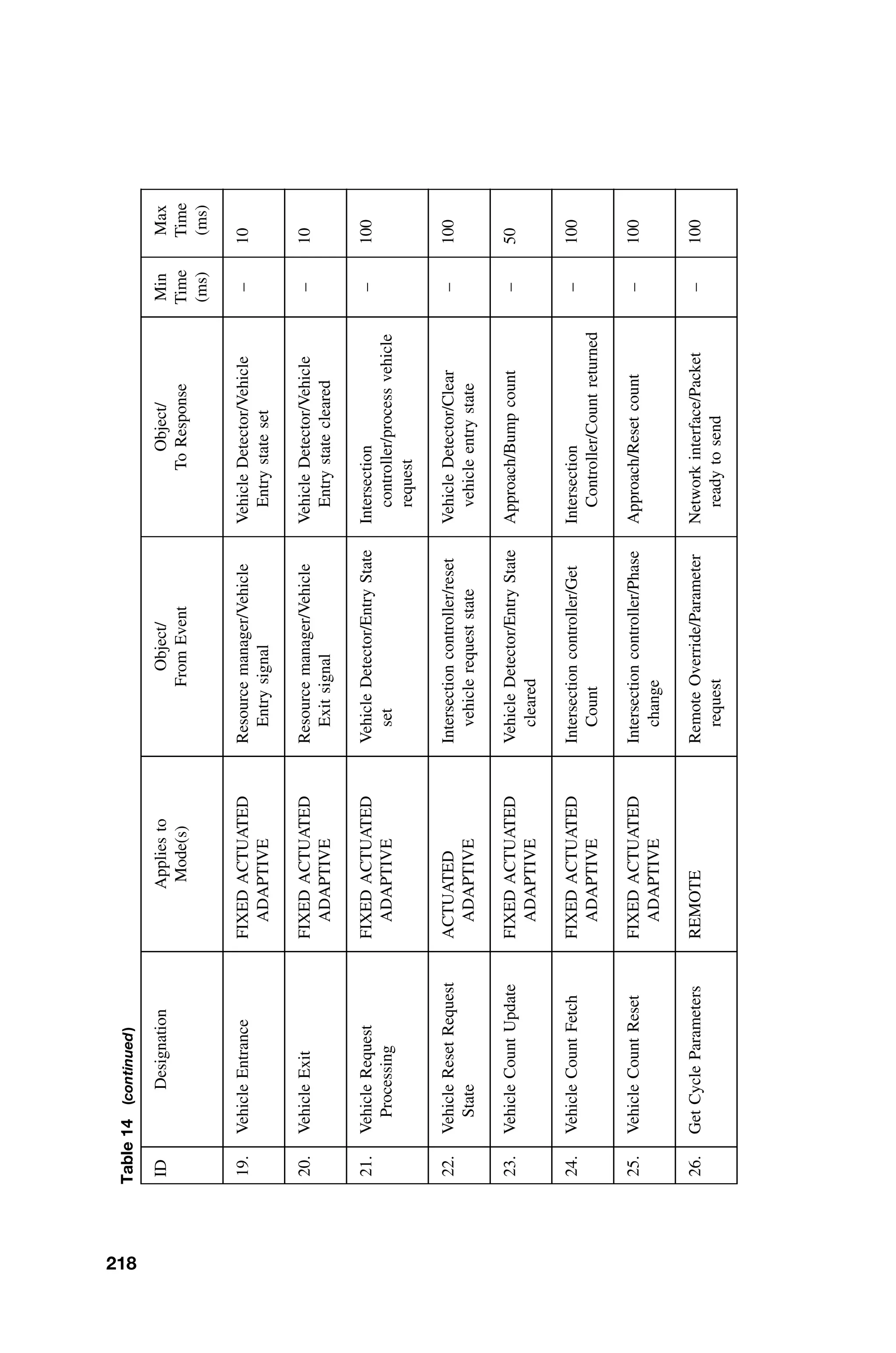
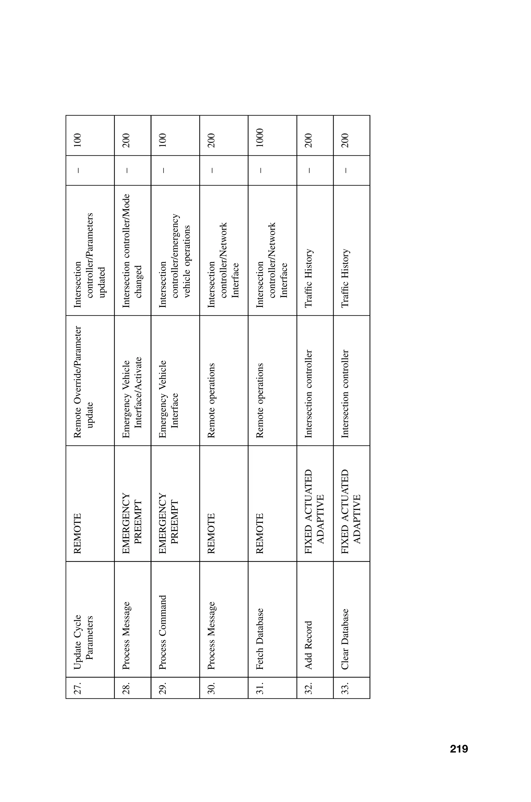
![(continued
)
ID
Designation
Applies
to
Mode(s)
Object/
From
Event
Object/
To
Response
Min
Time
(ms)
Max
Time
(ms)
34.
Add
Record
FIXED
ACTUATED
ADAPTIVE
Intersection
controller
Incident
Log
–
200
35.
Clear
Database
FIXED
ACTUATED
ADAPTIVE
Intersection
controller
Incident
Log
–
200
Notes:
[1]
The
timing
requirements
for
vehicle
detection
are
based
on
the
following
considerations:
Minimum
vehicle
length
=
8
ft
Minimum
following
distance
in
motion
=
4
ft
Loop
width
=
4
ft
Loop
detects
entrance
with
leading
overlap
=
2
ft
Loop
detects
exit
with
trailing
overlap
=
1
ft
Maximum
vehicle
speed
=
65
mph(=
95.3
ft/s)
Vehicle
speed
for
minimum
gap
time
(see
below)
=
10
mph
(=
14.67
ft/s)
Minimum
presence
pulse
width
=
9
ft/95.3
ft/s
=
94.4
ms
Minimum
gap
time
(time
between
exit
and
next
vehicle
entrance)
=
3
ft/14.67
ft/s
=
204.5
ms
220](https://image.slidesharecdn.com/epdf-230618090952-bdcb6616/75/epdf-pub_real-time-systems-design-and-analysis-pdf-243-2048.jpg)
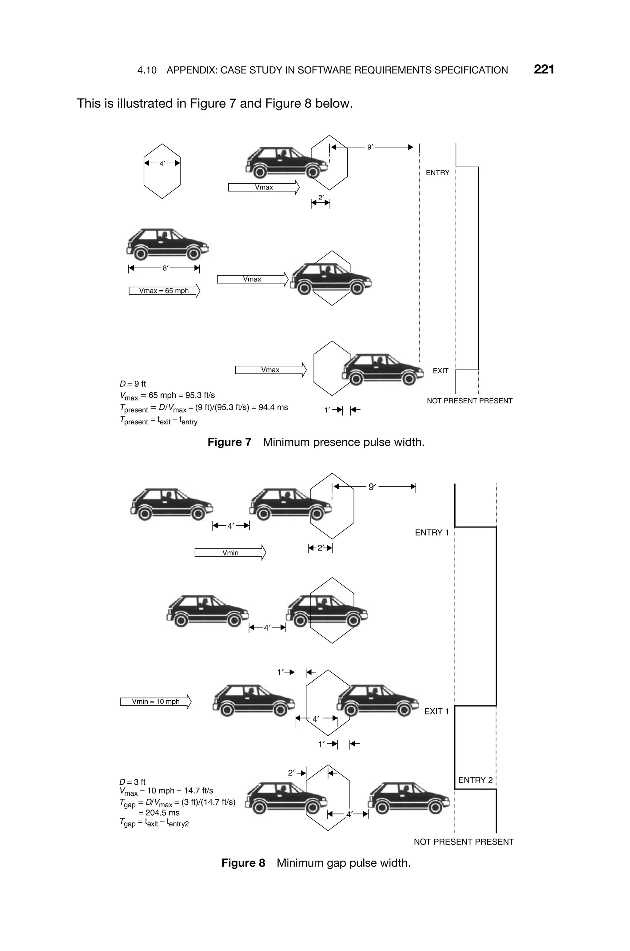
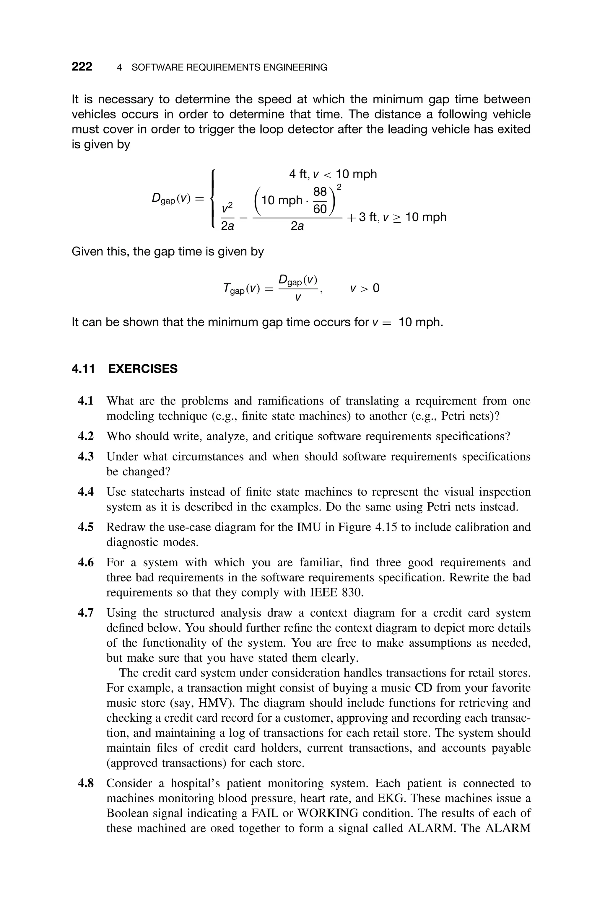


![5.1 PROPERTIES OF SOFTWARE 227
Another way to characterize software reliability is in terms of a real-valued
failure function. One failure function uses an exponential distribution where the
abscissa is time and the ordinate represents the expected failure intensity at that
time (Equation 5.2).
f (t) = λe−λt
t ≥ 0 (5.2)
Here the failure intensity is initially high, as would be expected in new software,
as faults are detected during testing. However, the number of failures would
be expected to decrease with time, presumably as failures are uncovered and
repaired (Figure 5.1). The factor λ is a system-dependent parameter.
A second failure model is given by the “bathtub curve” shown in Figure 5.2.
Brooks notes that while this curve is often used to describe the failure function
of hardware components, it might also be useful in describing the number of
errors found in a certain release of a software product [Brooks95].
The interpretation of this failure function is clear for hardware; a certain num-
ber of product units will fail early due to manufacturing defects. Later, the failure
intensity will increase as the hardware ages and wears out. But software does not
wear out. If systems seem to fail according to the bathtub curve, then there has
to be some plausible explanation.
It is clear that a large number of errors will be found early in a particular
software product, just as in the exponential model of failure. But why would the
failure intensity increase much later? There are at least three possible explana-
tions. The first is that the errors are due to the effects of patching the software for
Failures
Detected
Time
l
Figure 5.1 An exponential model of failure represented by the failure function
f(t) = λe−λt
, t ≥ 0. Here λ is a system-dependent parameter [Laplante03c].](https://image.slidesharecdn.com/epdf-230618090952-bdcb6616/75/epdf-pub_real-time-systems-design-and-analysis-pdf-250-2048.jpg)
![228 5 SOFTWARE SYSTEM DESIGN
Time
l
Failures
Detected
Figure 5.2 A software failure function represented by the bathtub curve [Laplante03c].
various reasons. The second reason is that late software failures are really due
to failure of the underlying hardware. Finally, additional failures could appear
because of the increased stress on the software by expert users. That is, as users
master the software and begin to expose and strain advanced features, it is possi-
ble that certain poorly tested functionality of the software is beginning to be used.
Often the traditional quality measures of mean time to first failure (MTFF) or
mean time between failures (MTBF) are used to stipulate reliability in the soft-
ware requirements specification. This approach to failure definition places great
importance on the effective elicitation (gathering) and specification of functional
requirements, because the requirements define the software failure.
5.1.2 Correctness
Software correctness is closely related to reliability, and the terms are often used
interchangeably. The main difference is that minor deviation from the require-
ments is strictly considered a failure and hence means the software is incorrect.
However, a system may still be deemed reliable if only minor deviations from
the requirements are experienced. In real-time systems correctness incorporates
correctness of outputs and deadline satisfaction. This definition is closer to the
formal methods definition of correctness in terms of correctness of outputs if the
software halts and establishing that the software halts.
5.1.3 Performance
Performance is a measure of some required behavior. One method of measur-
ing performance is based on mathematical or algorithmic complexity, either in](https://image.slidesharecdn.com/epdf-230618090952-bdcb6616/75/epdf-pub_real-time-systems-design-and-analysis-pdf-251-2048.jpg)
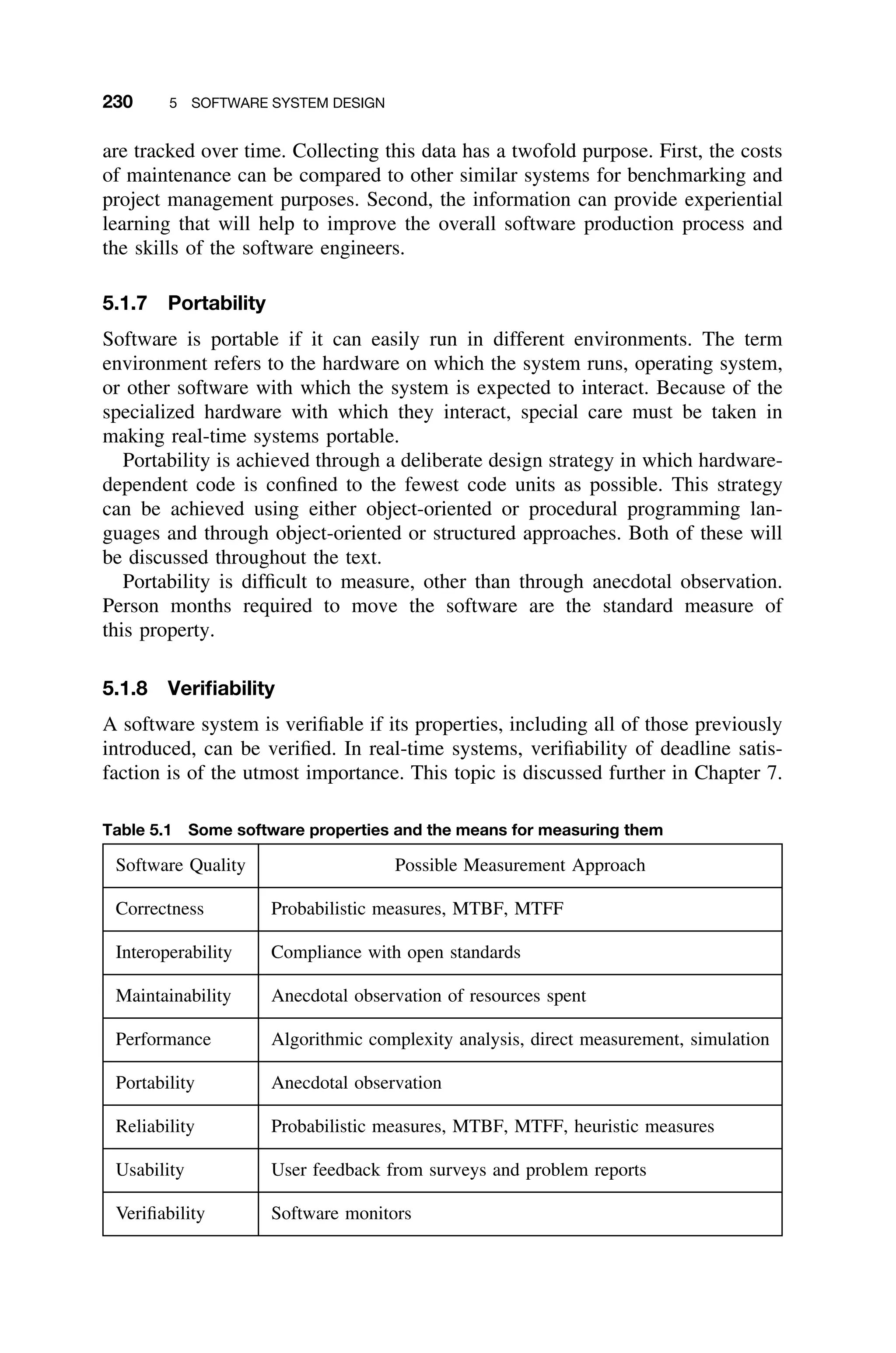
![232 5 SOFTWARE SYSTEM DESIGN
5.2.3 Modularity
Some separation of concerns can be achieved in software through modular design.
Modular design involves the decomposition of software behavior in encapsulated
software units, and can be achieved in either object-oriented or procedurally
oriented programming languages.
Modularity is achieved by grouping together logically related elements, such as
statements, procedures, variable declarations, and object attributes, in an increas-
ingly fine-grained level of detail (Figure 5.3). The main benefit of modularity is
high cohesion and low coupling. With respect to the code units, cohesion repre-
sents intramodule connectivity and coupling represents intermodule connectivity.
Coupling and cohesion can be illustrated informally as in Figure 5.4, which shows
software structures with high cohesion and low coupling (a) and low cohesion
and high coupling (b). The inside squares represent statements or data, arcs indi-
cate functional dependency. Cohesion relates to the relationship of the elements
of a module. High cohesion implies that each module represents a single part of
the problem solution. Therefore, if the system ever needs modification, then that
part that needs to be modified exists in a single place, making it easier to change.
Constantine and Yourdon identified seven levels of cohesion in order of strength
[Pressman00]:
Figure 5.3 Modular decomposition of code units. The arrows represent inputs and outputs
in the procedural paradigm. In the object-oriented paradigm they represent associations.
The boxes represent encapsulated data and procedures in the procedural paradigm. In the
object-oriented paradigm they represent classes [Laplante03c].](https://image.slidesharecdn.com/epdf-230618090952-bdcb6616/75/epdf-pub_real-time-systems-design-and-analysis-pdf-255-2048.jpg)
![5.2 BASIC SOFTWARE ENGINEERING PRINCIPLES 233
(a) (b)
Figure 5.4 Software structures with (a) high cohesion and low coupling and (b) low cohe-
sion and high coupling. The inside squares represent statements or data; arcs indicate
functional dependency.
ž Coincidental – Parts of module are not related, but simply bundled into a
single module.
ž Logical – Parts that perform similar tasks are put together in a module
ž Temporal – Tasks that execute within the same time span are brought
together.
ž Procedural – The elements of a module make up a single control sequence.
ž Communicational – All elements of a module act on the same area of a
data structure.
ž Sequential – The output of one part in a module serves as input for some
other part.
ž Functional – Each part of the module is necessary for the execution of a
single function.
Coupling relates to the relationships between the modules themselves. There
is a great benefit in reducing coupling so that changes made to one code unit do
not propagate to others, that is, they are hidden. This principle of “information
hiding,” also known as Parnas Partitioning, is the cornerstone of all software
design [Parnas79]. Low coupling limits the effects of errors in a module (lower
“ripple effect”) and reduces the likelihood of data-integrity problems. In some
cases, however, high coupling due to control structures may be necessary. For
example, in most graphical user interfaces control coupling is unavoidable, and
indeed desirable.
Coupling has also been characterized in increasing levels as:
1. No Direct Coupling – All modules are completely unrelated.
2. Data – When all arguments are homogeneous data items; that is, every
argument is either a simple argument or data structure in which all elements
are used by the called module.](https://image.slidesharecdn.com/epdf-230618090952-bdcb6616/75/epdf-pub_real-time-systems-design-and-analysis-pdf-256-2048.jpg)
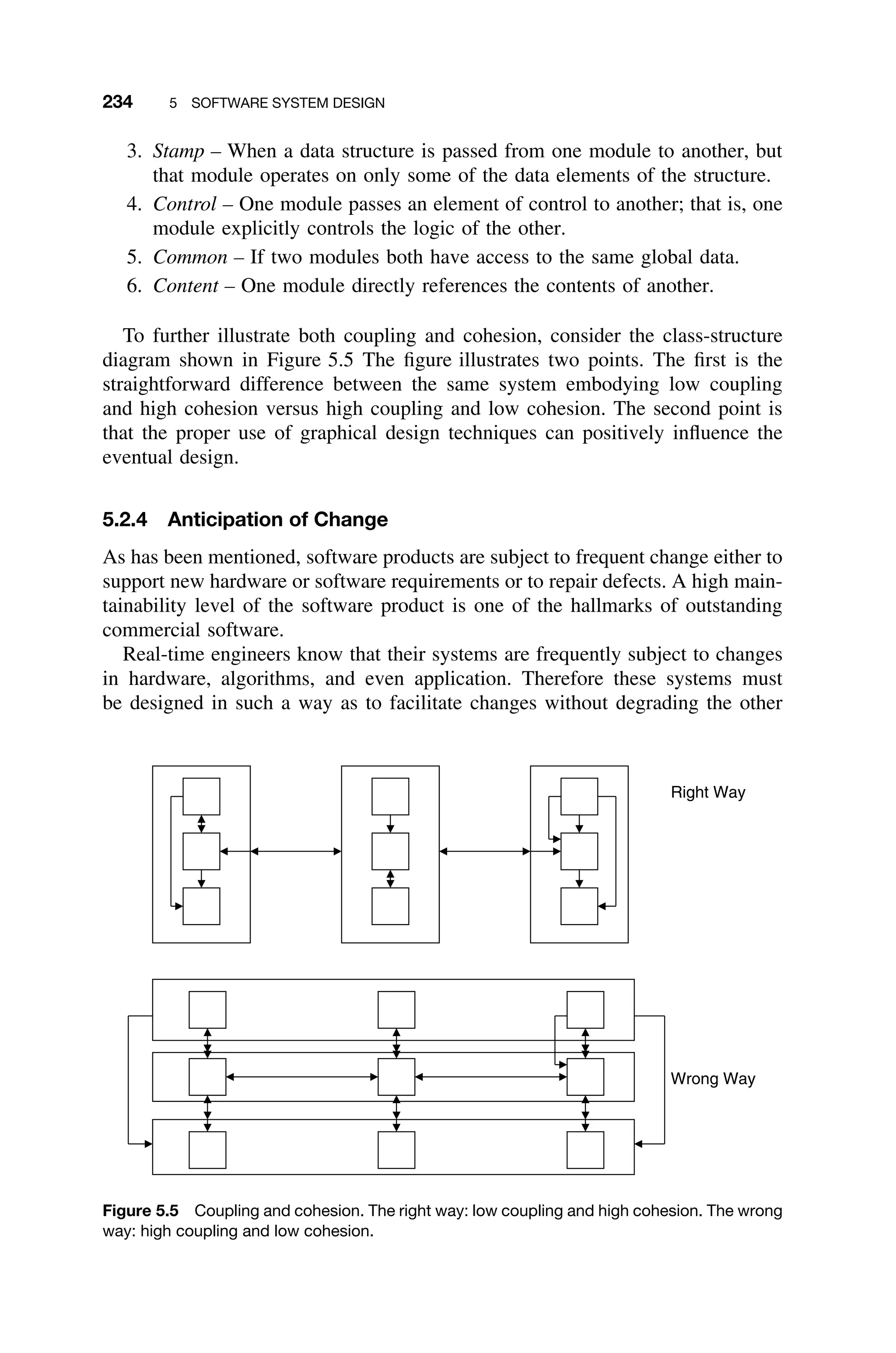
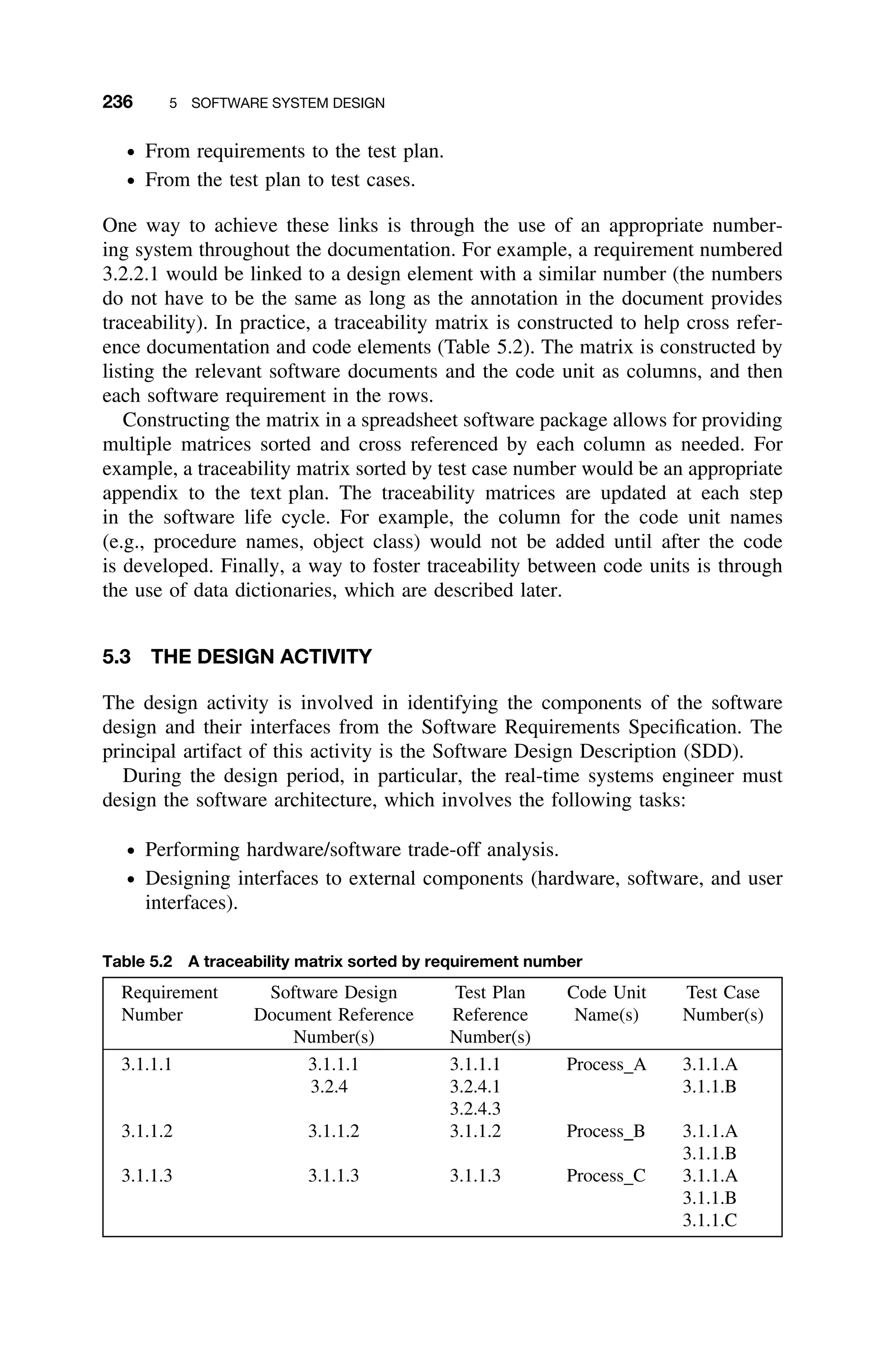
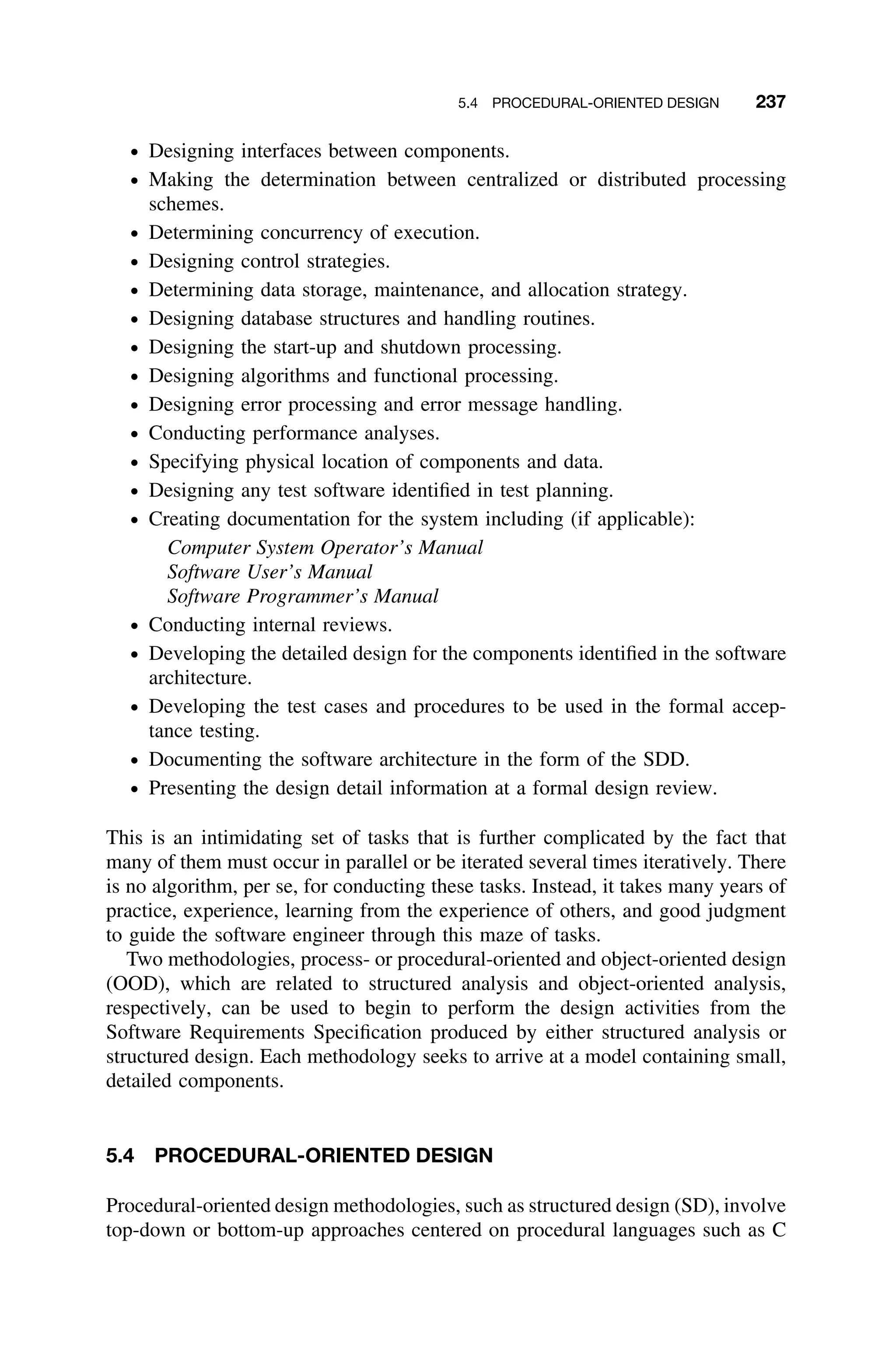
![238 5 SOFTWARE SYSTEM DESIGN
and Fortran. The most common of these approaches utilize design decomposition
via Parnas Partitioning.
5.4.1 Parnas Partitioning
Software partitioning into software units with low coupling and high cohesion
can be achieved through the principle of information hiding. In this technique, a
list of difficult design decisions or things that are likely to change is prepared.
Modules are then designated to “hide” the eventual implementation of each design
decision or feature from the rest of the system. Thus, only the function of the
module is visible to other modules, not the method of implementation. Changes
in these modules are therefore not likely to affect the rest of the system.
This form of functional decomposition is based on the notion that some aspects
of a system are fundamental, whereas others are arbitrary and likely to change.
Moreover, it is those arbitrary things, which are likely to change, that contain
“information.” Arbitrary facts are hard to remember and usually require lengthier
descriptions; therefore, they are the sources of complexity.
The following steps can be used to implement a design that embodies infor-
mation hiding.
1. Begin by characterizing the likely changes.
2. Estimate the probabilities of each type of change.
3. Organize the software to confine likely changes to a small amount of code.
4. Provide an “abstract interface” that abstracts from the differences.
5. Implement “objects,” that is, abstract data types and modules that hide
changeable data structures.
These steps reduce coupling and increase module cohesion. Parnas also indi-
cated that although module design is easy to describe in textbooks, it is difficult
to achieve. He suggested that extensive practice and examples are needed to
illustrate the point correctly [Parnas79].
As an example, consider a portion of the display function of a graphics system
associated with the nuclear monitoring system and shown in hierarchical form in
Figure 5.6. It consists of graphics that must be displayed (e.g., a representation
of the reactor core or sensor data) and are essentially composed from circles
and boxes. Different objects can also reside in different display windows. The
implementation of circles and boxes is based on the composition of line-drawing
calls. Thus, line drawing is the most basic hardware-dependent function. Whether
the hardware is based on pixel, vector, turtle, or other type of graphics does not
matter; only the line-drawing routine needs to be changed. Hence, the hardware
dependencies have been isolated to a single code unit.
Parnas partitioning “hides” the implementation details of software features,
design decisions, low-level drivers, and so on, in order to limit the scope of
impact of future changes or corrections. By partitioning things likely to change,
only that module needs to be touched when a change is required, without the](https://image.slidesharecdn.com/epdf-230618090952-bdcb6616/75/epdf-pub_real-time-systems-design-and-analysis-pdf-261-2048.jpg)
![5.4 PROCEDURAL-ORIENTED DESIGN 239
Images
Window
Box
Line
Circle
Line
Pixel, Vector,
Turtle, etc.
Figure 5.6 Parnas Partitioning of graphics rendering software [Laplante03c].
need to modify unaffected code. This technique is particularly applicable and
useful in embedded systems; since they are so directly tied to hardware, it is
important to partition and localize each implementation detail with a particu-
lar hardware interface. This allows easier future modification due to hardware
interface changes and reduces the amount of code affected.
If in designing the software modules, increasing levels of detail are deferred
until later (subordinate code units), then the software the approach is top-down.
If, instead, the design detail is dealt with first and then increasing levels of
abstraction are used to encapsulate those details, then the approach is bottom-up.
For example in Figure 5.6, it would be possible to design the software by
first describing the characteristics of the various components of the system and
the functions that are to be performed on them, such as opening, closing, and
sizing windows. Then the window functionality could be broken down into its
constituent parts, such as boxes and text. These could be subdivided even further,
that is, all boxes consist of lines, and so on. The top-down refinement continues
until the lowest level of detail needed for code development has been reached.
Alternatively, it is possible to begin by encapsulating the details of the most
volatile part of the system, the hardware implementation of a single line or pixel,
into a single code unit. Then working upward, increasing levels of abstraction are
created until the system requirements are satisfied. This is a bottom-up approach
to design.
5.4.2 Structured Design
Structured design (SD) is the companion methodology to structured analysis.
Structured design is a systematic approach concerned with the specification of
the software architecture and involves a number of techniques, strategies, and
tools. SD provides a step-by-step design process that is intended to improve](https://image.slidesharecdn.com/epdf-230618090952-bdcb6616/75/epdf-pub_real-time-systems-design-and-analysis-pdf-262-2048.jpg)
![240 5 SOFTWARE SYSTEM DESIGN
software quality and reduce risk of failure, to increase reliability, flexibility,
maintainability, and effectiveness. The data flow diagrams (DFD) partition system
functions and document that partitioning inside the specification.
5.4.2.1 Transitioning from Structured Analysis to Structured Design
Structured analysis (SA) is related to SD in the same way that a requirements rep-
resentation is related to the software architecture, that is, the former is functional
and flat and the latter is modular and hierarchical. In this regard data structure
diagrams are used to give information about logical relationships in complex
data structures.
The transition mechanisms from SA to SD are manual and involve significant
analysis and trade-offs of alternative approaches. Normally, SD proceeds from
SA in the following manner. Once the context diagram is drawn, a set of DFDs is
developed. The first DFD, the level 0 diagram, shows the highest level of system
abstraction. Subdividing processes to lower and lower levels until they are ready
for detailed design renders new DFDs with successive levels of increasing detail.
This decomposition process is called leveling.
In a typical DFD boxes represent terminators that are labeled with a noun
phrase that describes the system, agent, or device from which data enters or to
which data exits. Each process depicted by a circle is labeled as a verb phrase
describing the operation to be performed on the data, although it may be labeled
with the name of a system or operation that manipulates the data. Solid arcs are
used to connect terminators to processes and between processes to indicate the
flow of data through the system. Each arc is labeled with a noun phrase that
describes the data. Dashed arcs are discussed later. Parallel lines indicate data
stores, which are labeled by a noun phrase naming the file, database, or repository
where the system stores data.
Each DFD should typically have between five and nine processes [DeMarco78].
The descriptions for the lowest level, or primitive, processes are called process
specifications, or P-SPECs, and are expressed in either structured English, pseu-
docode, decision tables, or decision trees, and are used to describe the logic
and policy of the program (Figure 5.7). For example, consider the inertial mea-
surement system and refer to its context diagram shown in Figure 4.26. The
associated level 0 DFD is shown in Figure 5.8.
Process 1 in the level 0 DFD can be further decomposed, as shown into the
level 1 DFD shown in Figure 5.9. In this case, short of the equations, DFD 1
for gyro torquing can be used to produce P-SPECs which would include the
necessary equations to convert the attitude adjustment to the appropriate number
of torquing pulses. These are shown in Figure 5.10.
Continuing with the example, DFD 2: processor accelerometer data is sown
in Figure 5.11. To illustrate a further decomposition, DFD 2.3 for compensate
accelerometer data is shown in Figure 5.12. Finally, an associated P-SPEC for
DFD 2.3 is given in Figure 5.13. In addition to the DFDs, SD uses a data
dictionary to document and control interfaces. Entity relationship diagrams are
frequently used to define the relationship between the components of the system,
much as in the object-oriented paradigm. The data dictionary documents each](https://image.slidesharecdn.com/epdf-230618090952-bdcb6616/75/epdf-pub_real-time-systems-design-and-analysis-pdf-263-2048.jpg)
![5.4 PROCEDURAL-ORIENTED DESIGN 241
Context Diagram
DFD Level 1
DFD Level 0
B
C
A
System
Part 1
Part 2
Part 3
X
Y
Z
e
X d
f
Y
Z Part 3.1
Part 3.2
Result
e
Z
f
P_Spec 3.2
Result: data_in;
Z: data_out;
Body
….
Figure 5.7 Context diagram evolution from context diagram to level 0 DFD to level 1 DFD,
and finally, to a P-SPEC, which is suitable for coding [Laplante03b].
DFD 0
Display Information
∆x, ∆y, ∆z
Torquing Pulses
(gx, gy, gz)
40a-ms Interrupt
Attitude Data
Attitude Data
Temperature, Other
Physical Data
Torque
Gyros
1
Process
Accelerometer
Data
2
10-ms
Interrupt
Store and
Transmit
Data
3
40b-ms
Interrupt
Diagnostics
4
True Acceleration,
Velocity, and Position
Information
1000-ms
Interrupt
Temperature,
Other Physical
Data
True Acceleration,
Velocity, and Position
Information Diagnostics
Information
Diagnostics
Information
Diagnostics
Information
Figure 5.8 Level 0 DFD for the inertial measurement system. The dashed arcs represent
control flow in the system.](https://image.slidesharecdn.com/epdf-230618090952-bdcb6616/75/epdf-pub_real-time-systems-design-and-analysis-pdf-264-2048.jpg)
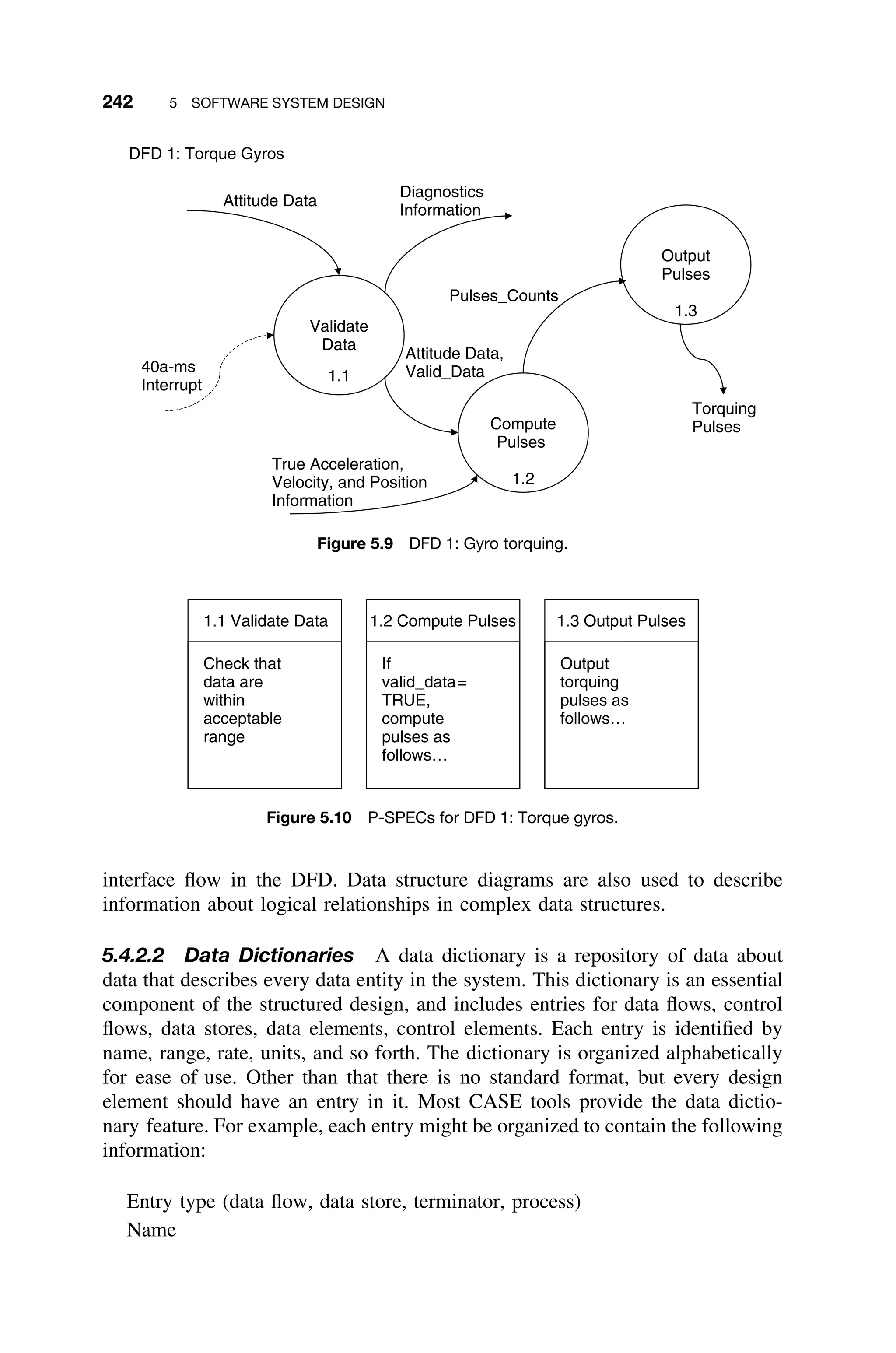
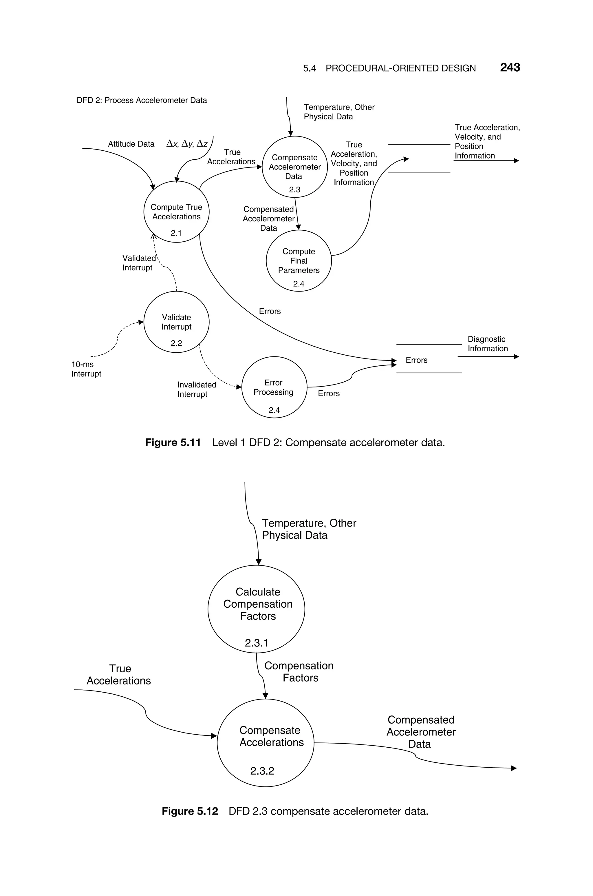
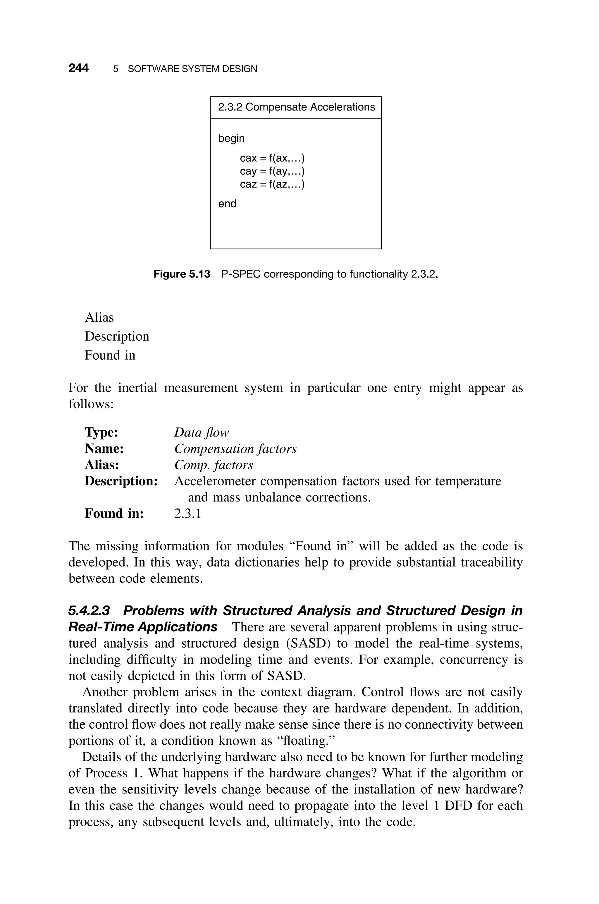
![5.4 PROCEDURAL-ORIENTED DESIGN 245
Clearly making and tracking changes in structured design is fraught with dan-
ger. Moreover, any change means that significant amounts of code would need
to be rewritten, recompiled, and properly linked with the unchanged code to
make the system work. None of these problems arise using the object-oriented
paradigm.
5.4.2.4 Real-Time Extensions of Structured Analysis and Structured
Design It is well known that the standard SASD methodology is not well
equipped for dealing with time, as it is a data-oriented and not a control-oriented
approach. In order to address this shortcoming, Hatley and Pirbhai extended the
SASD method by allowing for the addition of control flow analysis. To do this
the following artifacts were added to the standard approach: arcs made of dashed
lines to indicate the flow of control information, and solid bars indicating “stored”
control commands (control stores), which are left unlabeled [Hatley87].
Additional tools, such as Mealy finite state machines, are used to represent the
encapsulated behavior and process activations. The addition of the new control
flows and control stores allow for the creation of a diagram containing only those
elements called a control flow diagram (CFD). These CFDs can be decomposed
into C-SPECs (control specifications), which can then be described by a finite
state machine. The relationship between the control and process models is shown
in Figure 5.14. Although the Hatley-Pirbhai extensions suggest that the CFD and
C-SPECs stand alone, the CFD by itself makes little sense. Hence, the CFD and
DFD are generally combined as shown in Figure 5.11.
Process Model
DFDs
P-SPECs
Control Model
C-SPECs
CFDs
Data Outputs
Data Inputs
Control
Inputs
Control
Outputs
Process
Activations
Data
Conditions
Figure 5.14 The relationship between the control and process model [Laplante03c].](https://image.slidesharecdn.com/epdf-230618090952-bdcb6616/75/epdf-pub_real-time-systems-design-and-analysis-pdf-268-2048.jpg)
![246 5 SOFTWARE SYSTEM DESIGN
5.4.3 Design in Procedural Form Using Finite State Machines
One of the advantages of using finite state machines in the software requirements
specification and later in the software design is that they are easily converted to
code and test cases. For example, consider the inertial measurement system. The
tabular representation of the state transition function (Table 4.2), which describes
the system’s high-level behavior, can be easily transformed into a design using the
pseudocode shown in Figure 5.15. Each procedure associated with the operational
modes (TAK, NAV, NAE, NAA, LAN) will be structured code that can be viewed
as executing in one of any number of process states at an instant in time. This
functionality can be described by the pseudocode shown in Figure 5.15.
The pseudocode shown in Figures 5.15 and 5.16 can be coded easily in any
procedural language, or even an object-oriented one. Alternatively, the system
behavior can be described with a case statement or nested if then statements
such that, given the current state and receipt of a signal, a new state is assigned.
This is illustrated below:
TAK:
If MA then NAV
Else TAK
NAV:
If TD then NAA
If MC then LAN
If LO then NAE
Else NAV
typedef states: (state 1,...,state n); {n is# of states}
alphabet: (input 1,...,input n);
table_row: array [1..n] of states;
procedure move_forward; {advances FSM one state}
var
state: states;
input: alphabet;
table: array [1..m] of table_row; {m is the size of the alphabet}
begin
repeat
get(input); {read one token from input stream}
state:=table[ord(input)] [state]; {next state}
execute_process (state);
until input = EOF;
end;
Figure 5.15 Pseudocode that can implement the behavior of the finite state machine shown
in Figure 4.1 [Laplante03c].](https://image.slidesharecdn.com/epdf-230618090952-bdcb6616/75/epdf-pub_real-time-systems-design-and-analysis-pdf-269-2048.jpg)
![5.5 OBJECT-ORIENTED DESIGN 247
Procedure execute_process (state: states);
begin
case state of
state 1: process 1; {execute process 1}
state 2: process 2; {execute process 2}
...
state n: process n; {execute process n}
end
Figure 5.16 Finite state machine code for executing a single operational process in the
avionics system. Each process can exist in multiple states, allowing for partitioning of the code
into appropriate modules [Laplante03c].
NAE:
If EE then NAA
Else NAE
NAA:
If LO then NAE
If ED then NAV
Else NAA
LAN:
Else LAN
The advantage of finite state machine design over the case statement, of course,
is that the former is more flexible and compact.
5.5 OBJECT-ORIENTED DESIGN
Object-oriented programming languages are those characterized by data
abstraction, inheritance, polymorphism and messaging. Data abstraction was
defined earlier. Inheritance allows the software engineer to define new objects in
terms of previously defined objects so that the new objects “inherit” properties.
Function polymorphism allows the programmer to define operations that behave
differently, depending on the type of object involved. Messaging allows objects
to communicate and invoke the methods that they support.
Object-oriented languages provide a natural environment for information hid-
ing through encapsulation. The state, data, and behavior of objects are encapsu-
lated and accessed only via a published interface or private methods. For example,
in the inertial measurement system it would be appropriate to design a class called
accelerometer with attributes describing its physical implementation and methods
describing its output, compensation, and so forth.
Object-oriented design is an approach to systems design that views the system
components as objects and data processes, control processes, and data stores that
are encapsulated within objects. Early forays into object-oriented design were led](https://image.slidesharecdn.com/epdf-230618090952-bdcb6616/75/epdf-pub_real-time-systems-design-and-analysis-pdf-270-2048.jpg)
![248 5 SOFTWARE SYSTEM DESIGN
by attempts to reuse some of the better features of conventional methodologies,
such as the DFDs and entity relationship models by reinterpreting them in the
context of object-oriented languages. This can be seen in the Unified Modeling
Language (UML). Over the last several years the object-oriented framework has
gained significant acceptance into the software engineering community.
5.5.1 Benefits of Object Orientation
The benefits of object orientation in combining data and behavior into an encap-
sulated entity have been discussed already. The real advantages of applying
object-oriented paradigms are the future extensibility and reuse that can be
attained, and the relative ease of future changes.
Software systems are subject to near-continuous change: requirements change,
merge, emerge, and mutate; target languages, platforms, and architectures change;
and most significantly the way the software is employed in practice changes. This
flexibility places a considerable burden on the software design: How can systems
that must support such widespread change be built without compromising quality?
There are four basic principles of object-oriented engineering that can answer this
question and they have been recognized as supporting reuse.
5.5.1.1 Open–Closed Principle First recorded by Meyer [Meyer00], the
open–closed principle (OCP) states that classes should be open to extension, but
closed to modification. That is, it should be possible to extend the behavior of
a class in response to new or changing requirements, but modification to the
source code is not allowed. While these expectations may seem at odds, the
key is abstraction. In object-oriented systems a superclass can be created that
is fixed, but can represent unbounded variation by subclassing. This aspect is
clearly superior to structured approaches and top-down design in, for example,
changes in accelerometer compensation algorithms, which would require new
function parameter lists and wholesale recompilation of any modules calling that
code in the structured design.
5.5.1.2 Once and Only Once While certainly not a new idea, Beck [Beck99]
put a name to the principle that any aspect of a software system – be it an algo-
rithm, a set of constants, documentation, or logic – should exist in only one place.
This isolates future changes, makes the system easier to comprehend and main-
tain, and through the low coupling and high cohesion that the principle instills,
the reuse potential of these aspects increases. The encapsulation of state and
behavior in objects, and the ability to inherit properties between classes allows
for the rigorous application of these ideas in an object-oriented system, but is
difficult to implement in structured techniques. More importantly, in structured
techniques, once and only once (OAOO) needs to be breeched frequently for
reasons of performance, reliability, availability, and often, for security.
5.5.1.3 Dependency Inversion Principle The dependency inversion prin-
ciple (DIP) states that high-level modules should not depend upon low-level](https://image.slidesharecdn.com/epdf-230618090952-bdcb6616/75/epdf-pub_real-time-systems-design-and-analysis-pdf-271-2048.jpg)
![5.5 OBJECT-ORIENTED DESIGN 249
modules. Both should depend upon abstractions. This can be restated as: Abstrac-
tions should not depend upon details, details should depend upon abstractions.
Martin introduced this idea as an extension to OCP with reference to the prolifer-
ation of dependencies that exist between high- and low-level modules [Martin96].
For example, in a structured decomposition approach, the high-level procedures
reference the lower-level procedures, but changes often occur at the lowest levels.
This infers that high-level modules or procedures that should be unaffected by
such detailed modifications may be affected due to these dependencies. Again,
consider the case where the accelerometer characteristics change and even though
perhaps only one routine needs to be rewritten, the calling module(s) need to be
modified and recompiled as well. A preferable situation is to reverse these depen-
dencies, as is evident in the Liskov substitution principle (LSP). The intent here
is to allow dynamic changes in the preprocessing scheme, which is achieved by
ensuring that all the accelerometer objects conform to the same interface, and
are therefore interchangeable.
5.5.1.4 Liskov Substitution Principle Liskov expressed the principle of
the substitutivity of subclasses for their base classes as:
What is wanted here is something like the following substitution property: If for
each object o1 of type S there is an object o2 of type T such that for all programs P
defined in terms of T, the behavior of P is unchanged when o1 is substituted for o2
then S is a subtype of T. [Liskov88]
This principle has led to the concept of type inheritance and is the basis of
polymorphism in object-oriented systems, where instances of derived classes can
be substituted for each other, provided they fulfill the obligations of a com-
mon superclass.
5.5.2 Design Patterns
Developing software is hard and developing reusable software is even harder.
Designs should be specific to the current problem, but general enough to address
future problems and requirements. Experienced designers know not to solve every
problem from first principles, but to reuse solutions encountered previously, that
is, they find recurring patterns and use them as a basis for new designs. This is
simply an embodiment of the principle of generality.
While object-oriented systems can be designed to be as rigid and resistant to
extension and modification as in any other paradigm, object-orientation has the
ability to include distinct design elements that can cater to future changes and
extensions. These “design patterns” were first introduced to the mainstream of
software engineering practice by Gamma, Helm, Johnson, and Vlissides, and are
commonly referred to as the “Gang of Four (GoF)” patterns [Gamma94].
The formal definition of a pattern is not consistent in the literature. Sim-
ply, a pattern is a named problem–solution pair that can be applied in new](https://image.slidesharecdn.com/epdf-230618090952-bdcb6616/75/epdf-pub_real-time-systems-design-and-analysis-pdf-272-2048.jpg)
![250 5 SOFTWARE SYSTEM DESIGN
contexts, with advice on how to apply it in novel situations. This text is con-
cerned with three pattern types: architectural patterns, design patterns, and idioms.
An architectural pattern occurs across subsystems; a design pattern occurs within
a subsystem, but is independent of the language; an idiom is a low-level pattern
that is language specific.
In general, a pattern consists of four essential elements: a name, such as
“strategy,” “bridge,” “façade”; the problem to be solved; the solution to the
problem; and the consequences of the solution. More specifically, the problem
describes when to apply the pattern in terms of specific design problems, such
as how to represent algorithms as objects. The problem may describe class
structures that are symptomatic of an inflexible design. Finally, the problem
section might include conditions that must be met before it makes sense to apply
the pattern.
The solution describes the elements that make up the design, though it does
not describe a particular concrete design or implementation. Rather, the solution
provides how a general arrangement of objects and classes solves the problem.
Consider, for example, the previously mentioned GoF patterns. They describe
23 patterns, each organized by either creational, behavioral, or structural in its
intent (Table 5.3). Table 5.3 is provided for illustration only, and it is not the
intention to describe any of these patterns in detail. Other patterns have evolved,
particularly for real-time systems, that provide various approaches to addressing
the real-time communication and synchronization problem (e.g., [Douglass03;
Schmidt00]).
5.5.3 Object-Oriented Design Using the Unified Modeling Language
The UML is widely accepted as the de facto standard language for the specifica-
tion and design of software-intensive systems using an object-oriented approach.
By bringing together the “best-of-breed” in specification techniques, the UML
Table 5.3 The set of design patterns popularized by the
Gang of Four [Gamma94]
Creational Behavioral Structural
Abstract factory Chain of responsibility Adapter
Builder Command Bridge
Factory method Interpreter Composite
Prototype Iterator Decorator
Singleton Mediator Facade
Memento Flyweight
Observer Proxy
State
Strategy
Template method
Visitor](https://image.slidesharecdn.com/epdf-230618090952-bdcb6616/75/epdf-pub_real-time-systems-design-and-analysis-pdf-273-2048.jpg)
![5.5 OBJECT-ORIENTED DESIGN 251
has become a family of languages (diagram types), and users can choose which
members of the family are suitable for their domain.
The UML is a graphical language based upon the premise that any system can
be composed of communities of interacting entities and that various aspects of
those entities, and their communication can be described using the set of nine
diagrams: use case, sequence, collaboration, statechart, activity, class, object,
component, and deployment. Of these, five depict behavioral views (use case,
sequence, collaboration, statechart, and activity), while the remaining are con-
cerned with architectural or static aspects.
With respect to real-time systems it is these behavioral models that are of inter-
est. The use case diagrams document the dialog between external actors and the
system under development; sequence and collaboration diagrams describe inter-
actions between objects; activity diagrams illustrate the flow of control between
objects; and statecharts represent the internal dynamics of active objects. The
principle artifacts generated when using the UML and their relationships are
shown in Figure 5.17.
While not aimed specifically at embedded system design, some notion of time
has been included in the UML through the use of sequence diagrams. Other
modeling tools are needed, however. Statecharts and use case diagrams have
already been discussed, and the rest are introduced below. While discussed only
briefly below, many of these diagrams are illustrated in the extensive design case
study at the end of this chapter.
Application
Modeling
Requirements
Design
Use Case Model
Domain Model
Design Model
Concepts, Attributes,
and Associations
Software classes in domain
layer of design from concepts
in domain model
State Changes in Domain
Objects, Attributes, and
Associations
Class4
Class2
too()
bar()
Use
Cases
Use
Case
Diagrams
System
Sequence
Diagrams
System
Operation
Contracts
:System
System
Class1
Class3
Figure 5.17 The UML and its role in specification and design. (Adapted from [Larman02]).](https://image.slidesharecdn.com/epdf-230618090952-bdcb6616/75/epdf-pub_real-time-systems-design-and-analysis-pdf-274-2048.jpg)
![252 5 SOFTWARE SYSTEM DESIGN
5.5.3.1 Activity Activity diagrams are closely related to the flow chart and
are used for the same purpose, that is, to show flow of control. Typically, they
are used to model dynamic aspects of a system. However, unlike flowcharts, they
can model concurrent computational steps and the flow of objects as they move
from state to state at different points in the flow of control.
5.5.3.2 Class Diagram During system design the class diagram defines the
actual class attributes and methods implemented in an object-oriented program-
ming language. Design pattern architectures are explored and physical require-
ments assessed during design. Design patterns provide guidance on how the
defined class attributes, methods, and responsibilities should be assigned to objects.
Physical requirements require the programmer to revisit the analysis class dia-
gram where new classes for the system requirements are defined. Figure 10 in
the Appendix at the end of this chapter is a design class diagram for the traffic
intersection controller.
5.5.3.3 Collaboration Diagram Collaboration diagrams show the messages
passed between objects through the basic associations between classes. In essence,
they depict the behavior on class diagrams. Collaboration diagrams are the most
emphasized of UML interaction diagrams because of their clarity and expression
of more information. The collaboration diagram contains classes, associations,
and message flows between classes. Figures 4 through 9 in the Appendix at the
end of the chapter are collaboration diagrams for the traffic intersection controller.
5.5.3.4 Component These diagrams are made up of components, interfaces,
and relationships. Components represent preexiting entities. Interfaces represent
the functionality of components that are directly available to the user. Relation-
ships represent conceptual relationships between components [Holt01].
5.5.3.5 Deployment Deployment diagrams consist of nodes, representing
real-world aspects of a system and links that show relationships between nodes.
5.5.3.6 Object Diagram Object diagrams realize part of the static model of
a system and are closely related to class diagrams. They show the insides of
things in the class diagrams and their relationships. Moreover, they are a model
or snapshot of the run-time system at a given point in time.
5.5.3.7 Sequence Diagram Sequence diagrams are composed of three basic
elements: objects, links, and messages, which are exactly the same as for the
collaboration diagram. However, the objects shown in a sequence diagram have
a lifeline associated with them, which shows a logical time line. The time line is
present whenever the object is active, and is represented graphically as a vertical
line with logical time traveling down the line. The objects for the sequence
diagram are shown going horizontally across the page and are shown staggered
down the diagram depending on when they are created [Holt01]. Figure 13 in](https://image.slidesharecdn.com/epdf-230618090952-bdcb6616/75/epdf-pub_real-time-systems-design-and-analysis-pdf-275-2048.jpg)
![5.5 OBJECT-ORIENTED DESIGN 253
the Appendix at the end of the chapter illustrates the sequence diagram for the
traffic control system.
5.5.3.8 Modeling Time Explicitly It is clear from the previous description
that the UML in its current form does not provide sufficient facilities for the
specification and analysis of real-time systems. It is also stated, however, that
the UML is a family of languages, and there is no compelling reason for not
adding to the family if a suitable language is found. Unfortunately, the majority of
appropriate candidates are formal methods – specification languages with a sound
mathematical basis – and these are traditionally shunned by the user community.
As stated earlier, the domain model is created based upon the use cases and,
through further exploration of system behavior via the interaction diagrams, the
domain model evolves systematically into the design class diagram. The construc-
tion of the domain model is, therefore, analogous to the analysis stage in SASD
described earlier. In domain modeling the central objective is to represent the
real-world entities involved in the domain as concepts in the domain model. This
is a key aspect of object-oriented systems and is seen as a significant advantage
of the paradigm, since the resultant model is “closer” to reality than in alterna-
tive modeling approaches, including SASD. Part of the design class diagram that
results from evolution of the domain model is shown in Figure 5.15.
Most development in object-oriented design has been done with little or no
provision for real-time requirements. Two methodologies that do make such pro-
visions, real-time object-oriented modeling (ROOM) [Selic94] and HRT-HOOD
[Burns90] have gained some penetration into industry. But only HRT-HOOD
provides a method for guaranteeing deterministic timing behavior in hard real-
time systems. This is achieved by eliminating inheritance, introducing a small
number of class stereotypes (active, passive, protected, cyclic, and sporadic), and
restricting the synchronization mechanism for class operations [de la Puente00].
However, the Unified Process Model (UPM) with UML has been used success-
fully, with a number of extensions. And, as of this writing, UML 2.0, with
significant extensions for real-time applications, is about to be released.
5.5.3.9 Modeling Time in Object-Oriented Systems Behavioral aspects
of the design can be represented by a number of different diagrams in the UML.
Perhaps the most popular choice is to use sequence diagrams. Other techniques
for modeling time outside of the UML include the use of Q models [Motus94]
and various temporal logics.
5.5.3.10 Object-Oriented or Structured Design The preceding observa-
tions beg the question of whether object-oriented design is more suitable then SD
for the embedded real-time systems and the inertial measure unit in particular. SD
and object-oriented design are often compared and contrasted, and, indeed, they
are similar in some ways. This should be no surprise, since both have their roots
in the work of Parnas and his predecessors [Parnas79], [Parnas72]. Table 5.4
provides a side-by-side comparison of the methodologies.
Both structured and object-oriented analysis (OOA) are full life-cycle method-
ologies and use some similar tools and techniques. However, there are major](https://image.slidesharecdn.com/epdf-230618090952-bdcb6616/75/epdf-pub_real-time-systems-design-and-analysis-pdf-276-2048.jpg)
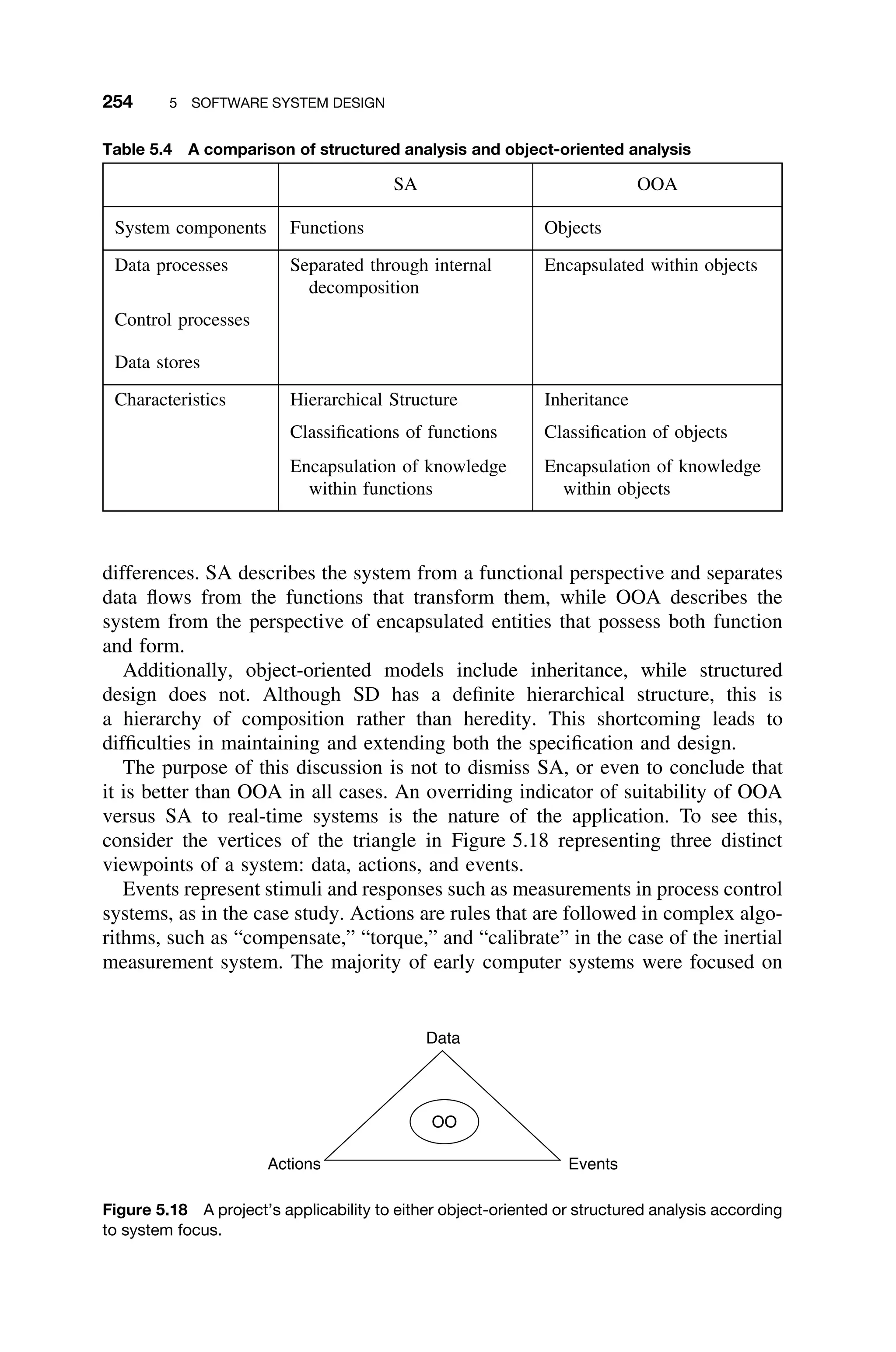
![256 5 SOFTWARE SYSTEM DESIGN
system can account for and respond to pedestrian traffic. The cycle is controlled by an
adaptive algorithm that uses data from many inputs to achieve maximum throughput
and acceptable wait-times for both pedestrians and motorists. A preempting feature
allows emergency vehicles to pass through the intersection in a safe and timely
manner by altering the state of the signals and the cycle time.
This document follows the structure provided in the object-oriented software
requirements specification (SRS) template found in IEEE 830-1999 ([2]) and adopted
in [1] rather than that defined in IEEE 1016-1998 ([3]) due to the fact that, as
acknowledged in the IEEE standard itself, IEEE 1016 is not suitable as a basis for
representing object-oriented designs.
1.3 Definitions and Acronyms
In addition to those given in [1], the following terms are defined here.
1.3.1 Accessor A method used to access a private attribute of an object.
1.3.2 Active Object An object that owns a thread and can initiate control activity.
An instance of active class.
1.3.3 Collaboration A group of objects and messages between them that interact
to perform a specific function.
As defined in [5], a collaboration is ‘‘The specification of how an operation or
classifier, such as a use case, is realized by a set of classifiers and associations
playing specific roles used in a specific way. The collaboration defines an interaction.’’
1.3.4 Mutator A method used to modify a private attribute of an object.
1.4 References
[1] T2-SRS Rev. A, ‘‘Software Requirements Specification (SRS) for an Intersec-
tion Traffic Control System.’’
[2] IEEE 830-1999.
[3] IEEE 1016-1998.
[4] Real Time UML, Second Edition- Developing Efficient Objects for Embedded
Systems, Bruce Powel Douglas, Addison-Wesley, New York, 1999.
[5] OMG Unified Modeling Language Specification, Version 1.4, September 2001.
2 OVERALL DESCRIPTION
2.1 Intersection Overview
The intersection class to be controlled is illustrated in Figure 1. This figure has been
repeated from [1].](https://image.slidesharecdn.com/epdf-230618090952-bdcb6616/75/epdf-pub_real-time-systems-design-and-analysis-pdf-279-2048.jpg)
![5.6 APPENDIX: CASE STUDY IN SOFTWARE REQUIREMENTS SPECIFICATION 257
SPEED
LIMIT
30
SPEED
LIMIT
55
OCCUPANCY
LOOP
N
E
S
W
PREVIOUS INTERSECTION (UPSTREAM)
NEXT INTERSECTION (DOWNSTREAM)
NEXT INTERSECTION (DOWNSTREAM)
ORTHOGONAL ROUTE
IDLE
AVENUE
(SECONDARY)
REAL TIME ROAD (ARTERIAL)
DIRECT ROUTE
All approaches are level,
tangent surfaces.
APPROACHES:
W-E
E-W
N-S
S-N
Figure 1 Intersection topography.
The target class of intersection is described in detail in [1].
2.2 Intersection Software Architecture
The intersection controller software architecture consists of the major components
shown in Figure 2.](https://image.slidesharecdn.com/epdf-230618090952-bdcb6616/75/epdf-pub_real-time-systems-design-and-analysis-pdf-280-2048.jpg)
![258 5 SOFTWARE SYSTEM DESIGN
Intersection Controller
RTOS
TCP/IP Stack() : void
POSIX Thread Management() : void
Resource Manager Interface() : void
Application
Software
init() : void
Network
Resource
Manager
Transponder
Resource
Manager
Other
Hardware
Resource
Managers
MaintenancePort
DOT WAN
Transponder
Other Hardware
Name: IntersectionController- System Architecture
Author: Team 2
Version: 1.0
Created: 09-Dec-2002 10:02:10
Updated: 09-Dec-2002 10:14:34
«depends»
«depends»
«depends»
SNMP
SNMP
«depends»
Figure 2 Intersection controller software architecture.
2.2.1 Real-Time Operating System (RTOS) The RTOS selected for the intersec-
tion controller is QNX Neutrino 6.2 for the iX86 family of processors.
2.2.2 Application Software Application software is written in C++ and is com-
piled using QNX Photon tools and the GNU gcc 2.95 compiler.
2.2.3 Resource Managers Resource managers are written in C++ using the
QNX Driver Development Kit. Note that these have been developed by another team
and so have not been covered in detail in this document.
3 DESIGN DECOMPOSITION
This section provides a detailed object-oriented decomposition of the intersection
controller software design. The decomposition is based on the use cases and
preliminary class model described in [1].
The decomposition makes use of the Unified Modeling Language (UML), supple-
mented by text descriptions, to define the details of the design. This representation
provides the design views described in IEEE 1016 ([3]) within the framework of
object-oriented design, as shown in Table 1.](https://image.slidesharecdn.com/epdf-230618090952-bdcb6616/75/epdf-pub_real-time-systems-design-and-analysis-pdf-281-2048.jpg)
![5.6 APPENDIX: CASE STUDY IN SOFTWARE REQUIREMENTS SPECIFICATION 259
Table 1 IEEE 1016 design views
Design View Represented By SDD Reference
Decomposition view Classes in class diagram Figure 10
Interrelationship view Associations in class diagram Figure 10
Interface view Collaboration diagrams Figure 4 through Figure 9
Detailed view Attribute and method details; behavioral
diagrams
For each class
3.1 Major Software Functions (Collaborations)
Based on the use case diagram provided in [1], the major functions of the intersection
controller have been grouped into UML collaborations (represented by dashed ovals)
as shown in Figure 3. Collaboration details are described in the following paragraphs.](https://image.slidesharecdn.com/epdf-230618090952-bdcb6616/75/epdf-pub_real-time-systems-design-and-analysis-pdf-282-2048.jpg)
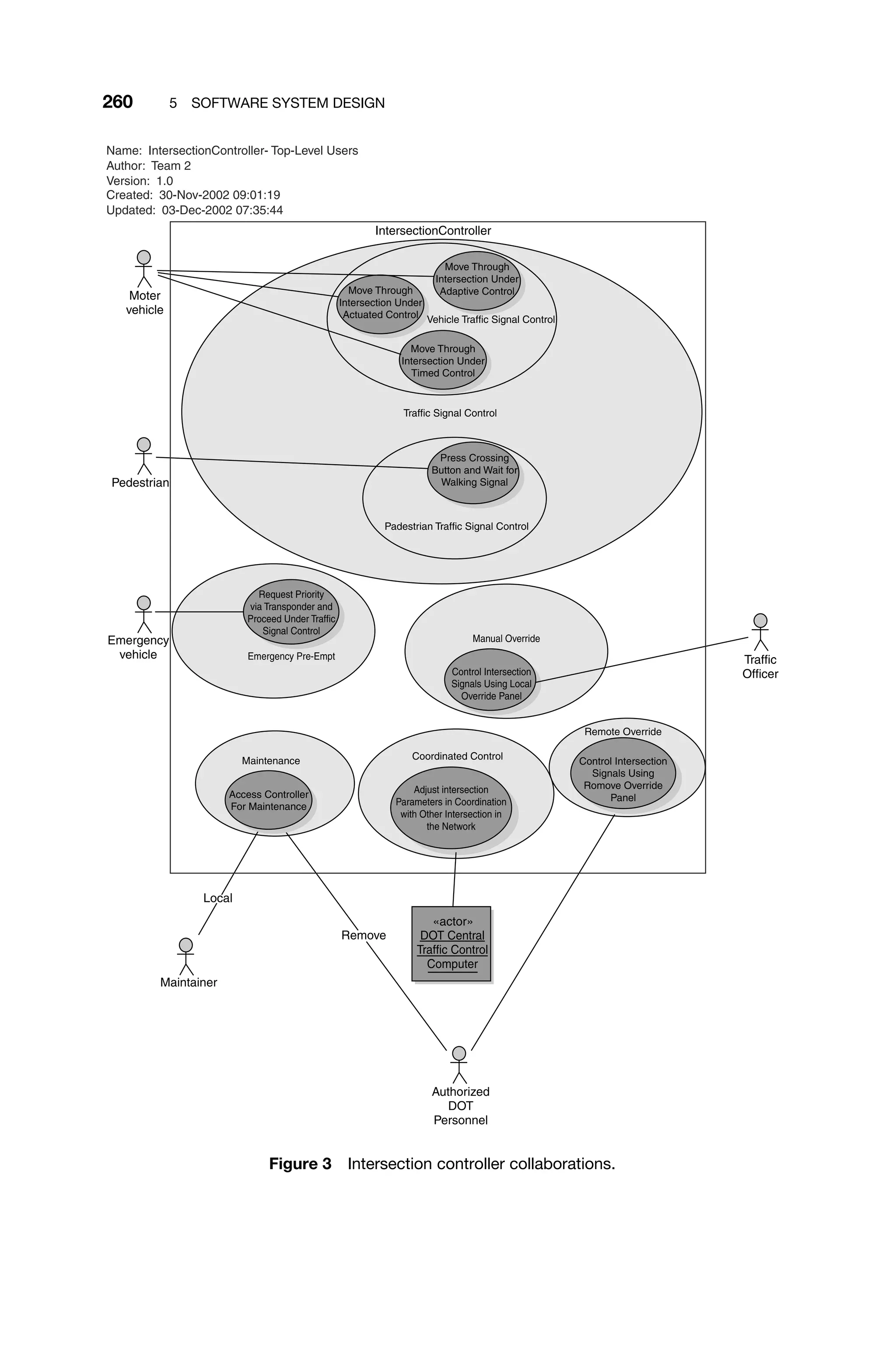
![5.6 APPENDIX: CASE STUDY IN SOFTWARE REQUIREMENTS SPECIFICATION 261
3.1.1 Collaboration Messages The tables below provide a listing of the mes-
sages (method calls and events) passed between objects in each collaboration
defined above. Messages with an ‘‘on. . .’’ prefix correspond to events.
3.1.1.1 Traffic Signal Control
Table 2 IntersectionController – traffic signal control collaboration messages
ID Message From Object To Object
1 setAspect(Aspect) m Intersection Controller m Approach[0]
1.1 getAspect() m Intersection Controller m Approach[0]
1.2 getCount() m Intersection Controller m Approach[0]
2 ignoreState() m Approach[0] m PedestrianDetector[0]
2.1 watchState() m Approach[0] m PedestrianDetector[0]
2.2 resetState() m Approach[0] m PedestrianDetector[0]
3 onEntryStateSet(void) m VehicleDetector m Approach[0]
3.1 onEntryStateCleared(void) m VehicleDetector m Approach[0]
4 onPedestrianRequest() m PedestrianDetector[0] m Approach[0]
5 onPedestrianRequest() m Approach[0] m Intersection Controller
5.1 onVehicleEntry(int) m Approach[0] m Intersection Controller
6 setIndication(Indication) m Approach[0] m PedestrianTrafficStandard[0]
6.1 getIndication() m Approach[0] m PedestrianTrafficStandard[0]
7 setIndication(Indication) m Approach[0] m VehicleTrafficStandard[0]
7.1 getIndication() m Approach[0] m VehicleTrafficStandard[0]
3.1.1.2 Emergency Preempt
Table 3 IntersectionController – emergency preempt collaboration messages
ID Message From Object To Object
1 onActivate() Emergency Vehicle Transponder m EmergencyPreempt
1.1 onDeactivate() Emergency Vehicle Transponder m EmergencyPreempt
2 onPreemptRequest() m EmergencyPreempt m Intersection Controller
(continued)](https://image.slidesharecdn.com/epdf-230618090952-bdcb6616/75/epdf-pub_real-time-systems-design-and-analysis-pdf-284-2048.jpg)
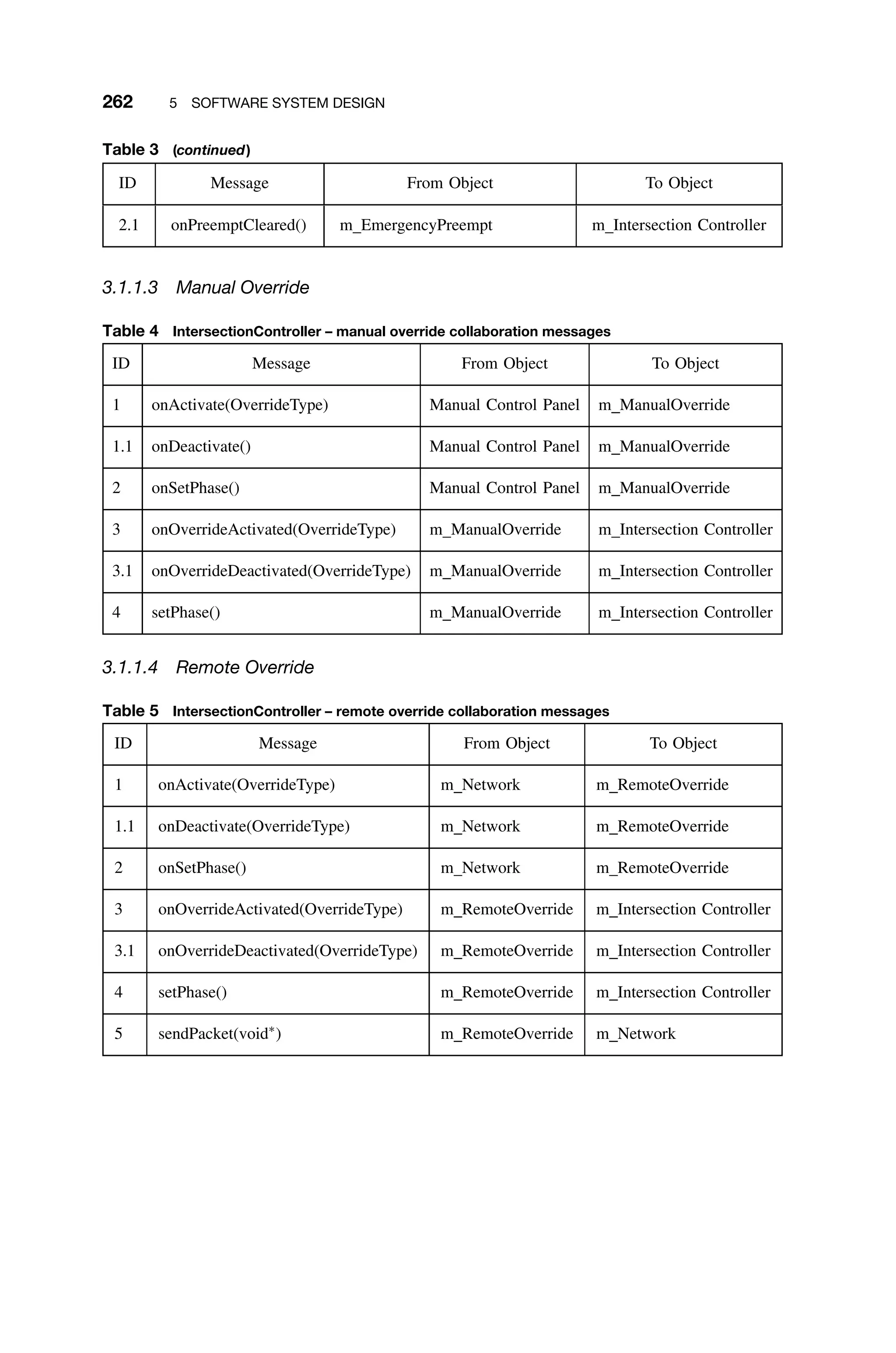
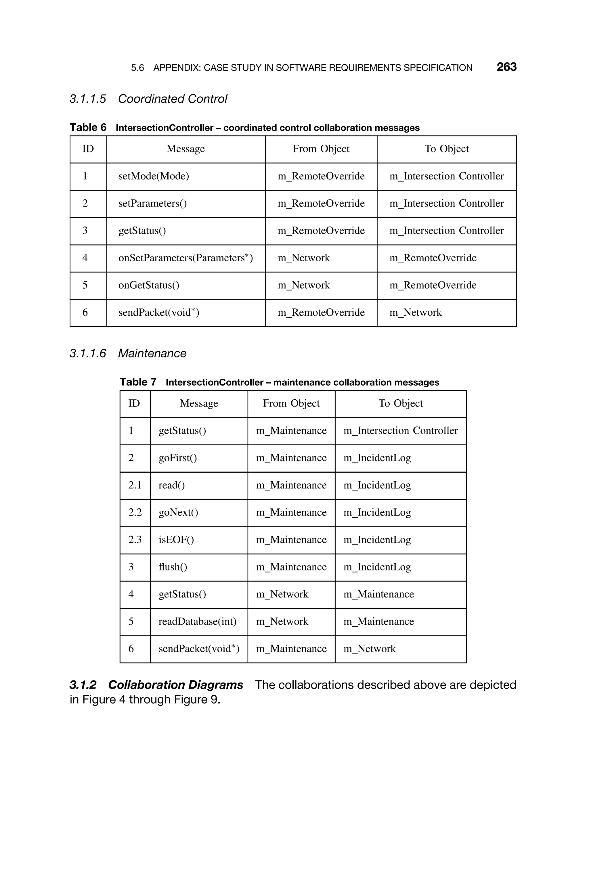
![264 5 SOFTWARE SYSTEM DESIGN
Same
messages
as
between
m_VehicleTrafficStandard[0]
and
m_Approach[0].
Same
messages
as
between
m_PedestrianTrafficStandard[0]
and
m_Approach[0].
Same
messages
as
between
m_PedestrianDetector[0]
and
m_Approach[0].
«singleton»
m_Intersection
Controller
:IntersectionController
m_Approach[0]
:Approach
m_Approach[1]
:Approach
m_Approach[2]
:Approach
m_Approach[3]
:Approach
m_PedestrianDetector[0]
:OnOffSensor
m_PedestrianDetector[1]
:OnOffSensor
m_VehicleDetector
:VehicleDetector
m_VehicleTrafficStandard[0]
:IntersectionStandard
m_VehicleTrafficStandard[1]
:IntersectionStandard
m_PedestrianTrafficStandard[0]
:IntersectionStandard
m_PedestrianTrafficStandard[1]
:IntersectionStandard
Other
Approach
objects
have
the
same
behavior
as
m_Approach[0].
Name:
IntersectionController-
Traffic
Signal
Control
Collaboration
Author:
Team
2
Version:
1.0
Created:
30-Nov-2002
18:30:05
Updated:
09-Dec-2002
08:03:00
1
setAspect(aspect)
1.1
m_Aspect:
=
getAspect()
1.2
m_Count:
=
getCount()
2
ignoreState()
2.1
watchState()
2.2
resetState()
3
onEntryStateSet(void)
3.1
onEntryStateCleared(void)
4
onPedestrianRequest()
5
onPedestrianRequest()
5.1
onVehicleEntry(approach)
6
setIndication(indication)
6.1
m_Indication:
=
getIndication()
7
setIndication(indication)
7.1
m_Indication:=
getIndication()
Figure
4
Traffic
signal
control.](https://image.slidesharecdn.com/epdf-230618090952-bdcb6616/75/epdf-pub_real-time-systems-design-and-analysis-pdf-287-2048.jpg)
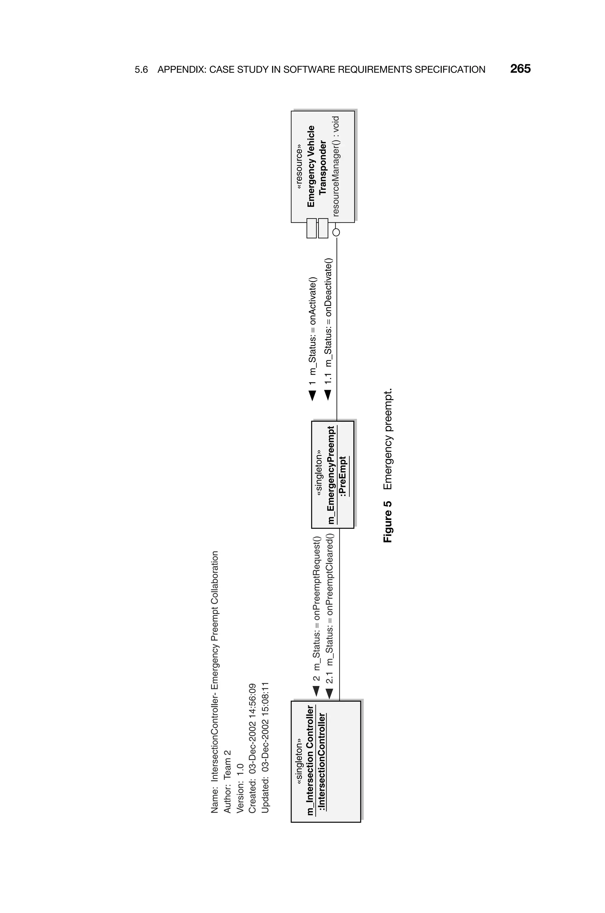
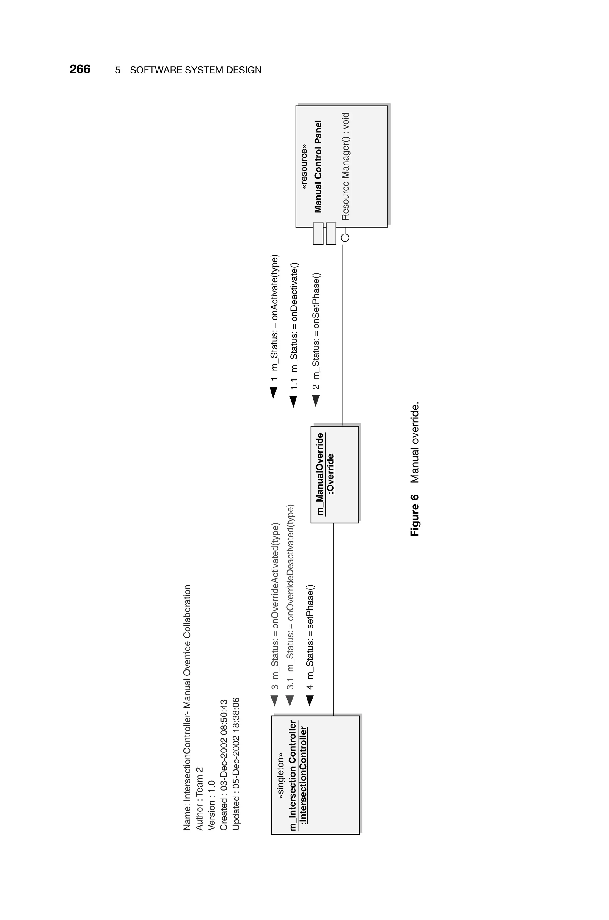
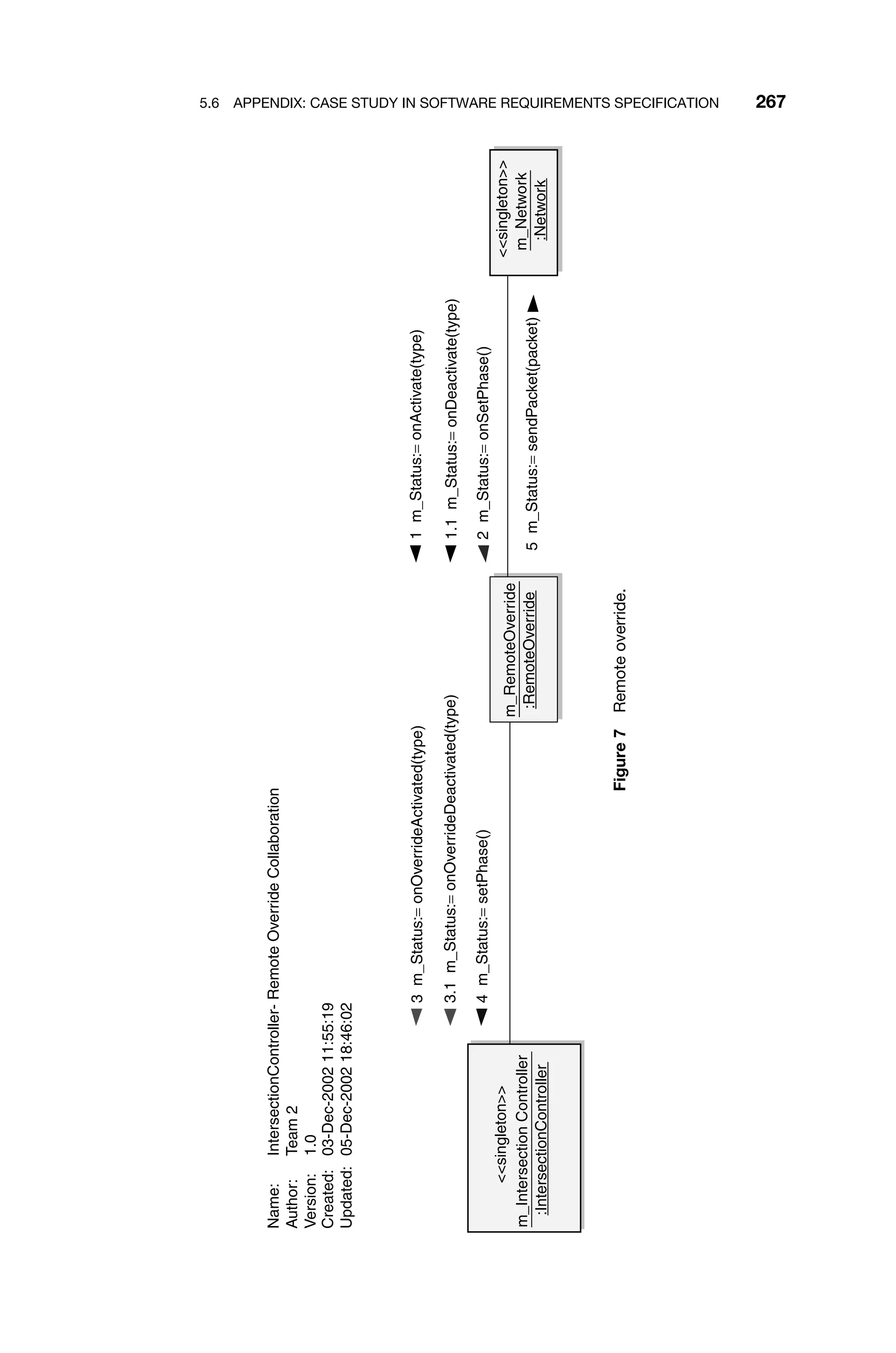
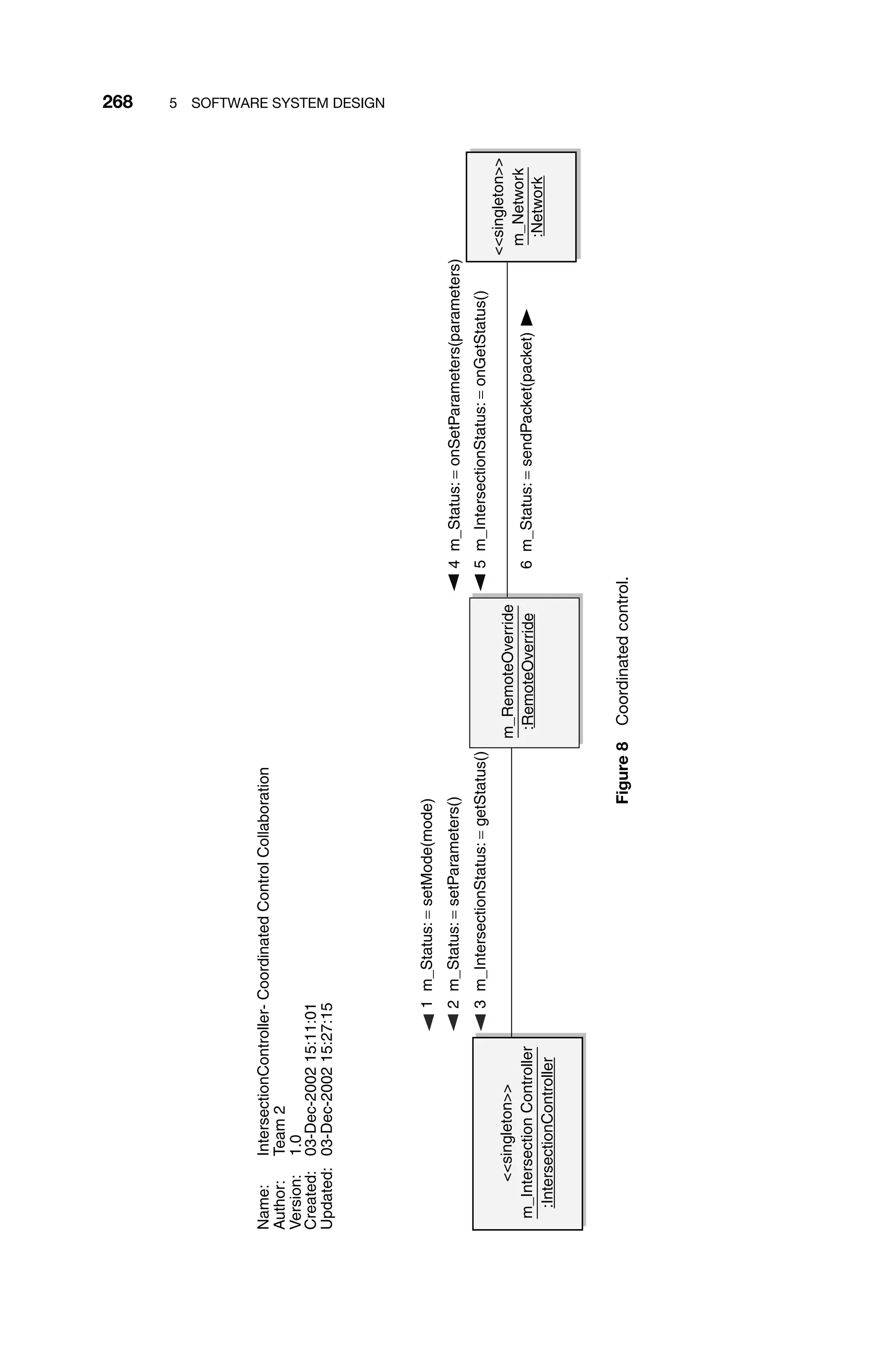
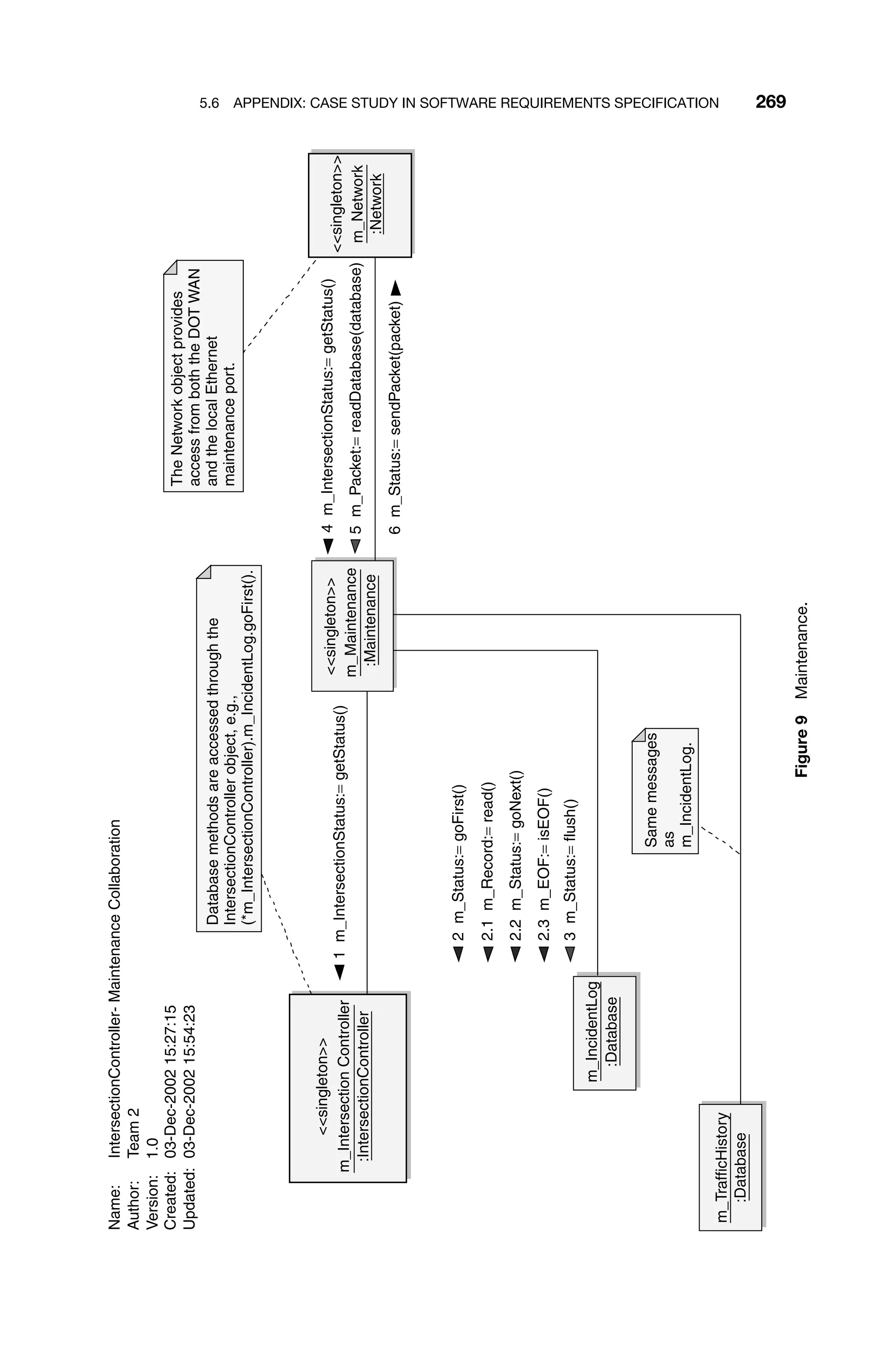
![270 5 SOFTWARE SYSTEM DESIGN
3.2 Class Model
Figure 10 depicts the classes constituting the intersection control system software
application. The diagram reflects the preliminary class structure defined in [1], but
with additional detail and, in some cases, addition of classes and reallocation of
responsibilities.](https://image.slidesharecdn.com/epdf-230618090952-bdcb6616/75/epdf-pub_real-time-systems-design-and-analysis-pdf-293-2048.jpg)
![5.6 APPENDIX: CASE STUDY IN SOFTWARE REQUIREMENTS SPECIFICATION 271
singleton
IntersectionController
−
NUMAPPROACHES:
int
=
4
−
m_Priority:
int
−
m_Mode:
Mode
−
m_CurrentPhase:
Phase*
−
m_ErrorHandler:
ErrorHandler*
−
m_Approach:
Approach*
[4
ordered]
−
m_Network:
Network*
−
m_EmergencyPreempt:
PreEmpt*
−
m_Parameters:
Parameters*
−
m_RemoteOverride:
RemoteOverride*
−
m_ManualOverride:
Override*
−
m_LocalTimeZone:
float
−
m_IncidentLog:
Database*
−
m_TrafficHistory:
Database*
−
m_Aspect:
Aspect*
−
m_Count:
int*
−
m_IntersectionStatus:
Status*
+
IntersectionController()
−*
∼
IntersectionController
()
−
init()
:
void
+
run()
:
void
+
setPhase()
:
int
+
setPhase(Phase)
:
int
+
getPhase()
:
Phase
+
checkPhase(Phase)
:
boolean
+
setCycle(float)
:
int
+
getCycle()
:
float
+
setSplits(Split*)
:
int
+
getSplits()
:
Split*
+
setMode(Mode)
:
int
+
getMode()
:
Mode
+
checkMode(Mode)
:
boolean
+
loadTimer(float)
:
int
+
onPreemptRequest()
:
int
+
onPreemptCleared()
:
int
+
onOverrideActivated(OverrideType)
:
int
+
onOverrideDeactivated(OverrideType)
:
int
+
toggleGreenSafetyRelay()
:
int
+
checkGreenSafetyRelay()
:
boolean
+
calculateParameters()
:
int
+
calculateTime(float,
Split*)
:
float
+
setParameters()
:
int
+
getParameters()
:
Parameters*
+
getStatus()
:
Status*
+
onPedestrianRequest()
:
void
+
onVehicleEntry(int)
:
void
Approach
{4}
−
m_CurrentAspect:
Aspect
−
m_PedestrianDetector:
OnOffSensor*
[2
ordered]
−
m_VehicleDetector:
VehicleDetector*
−
m_VehicleTrafficStandard:
IntersectionStandard*
[2
ordered]
−
m_PedestrianTrafficStandard:
IntersectionStandard*
[2
ordered]
−
m_Indication:
Indication*
[4
ordered]
−
m_Count:
int
−
m_SpeedLimit:
int
+
Approach()
−*
∼
Approach
()
+
setAspect(Aspect)
:
void
+
getAspect()
:
Aspect*
+
getCount()
:
int*
+
bumpCount(void)
:
void
+
clearCount(void)
:
void
+
onPedestrianRequest()
:
void
+
onEntryStateSet(void)
:
void
+
onEntryStateCleared(void)
:
void
enumeration
Phase
+
Default:
int
+
GG_GG_RR_RR:
int
+
GY_GY_RR_RR:
int
+
YR_YR_RR_RR:
int
+
RR_RR_RR_RR_4:
int
+
RR_RR_GG_GG:
int
+
RR_RR_GY_GY:
int
+
RR_RR_YR_YR:
int
+
RR_RR_RR_RR_8:
int
enumeration
Aspect
+
RR:
int
+
GG:
int
+
GY:
int
+
YR:
int
OnOffSensor
−
m_State:
boolean
−
m_IgnoreState:
boolean
+
OnOffSensor()
+*
∼
OnOffSensor
()
+
setState()
:
void
+
resetState()
:
void
+
ignoreState()
:
void
+
watchState()
:
void
VehicleDetector
+
VehicleDetector()
−*
~
VehicleDetector
()
IntersectionStandard
−
m_Stop:
boolean
−
m_Caution:
boolean
−
m_Go:
boolean
−
m_CurrentIndication:
Indication*
+
IntersectionStandard()
−*
∼
IntersectionStandard
()
+
setIndication(Indication)
:
void
+
getIndication()
:
Indication
Name:
IntersectionController-
Class
Model
Author:
Team
2
Version:
1.0
Created:
18-Nov-2002
16:34:46
Updated:
09-Dec-2002
07:13:36
enumeration
Indication
+
R:
int
+
Y:
int
+
G:
int
Override
−
m_IntersectionController:
IntersectionController*
+
Override()
−*
~
Override
()
+
onActivate(OverrideType)
:
int
+
onDeactivate(OverrideType)
:
int
+
onSetPhase()
:
int
RemoteOverride
−
m_Network:
Network*
+
RemoteOverride()
−*
~
RemoteOverride
()
+
onSetParameters(Parameters*)
:
int
+
onGetStatus()
:
Status*
Database
{2}
−
MAXRECORDS:
int
=
65536
−
m_Record:
Record*
[0..*
ordered
]
−
m_CurrentRecord:
int
−
m_First:
int
−
m_Last:
int
−
m_Full:
boolean
+
Database()
−*
∼
Database
()
+
goFirst()
:
int
+
goLast()
:
int
+
goNext()
:
int
+
go(int)
:
int
+
isFull()
:
boolean
+
isEOF()
:
boolean
+
read()
:
Record
+
read(int)
:
Record
+
write(Record*)
:
int
+
write(int,
Record*)
:
int
+
flush()
:
int
Record
−
timestamp:
datetime
−
source:
int
−
data:
string
+
Record()
−*
∼
Record
()
+
setTimestamp(datetime*)
:
void
+
setSource(int)
:
void
+
setData(string*)
:
void
+
getTimestamp()
:
datetime
+
getSource()
:
int
+
getData()
:
string
singleton
PreEmpt
−
m_IntersectionController:
IntersectionController*
+
PreEmpt()
−*
∼
PreEmpt
()
+
onActivate()
:
int
+
onDeactivate()
:
int
+
onTimeout()
:
void
enumeration
OverrideType
+
Manual:
int
+
Remote:
int
enumeration
Mode
+
Adaptive:
int
+
Actuated:
int
+
Timed:
int
+
Preempt:
int
+
Manual:
int
+
Remote:
int
+
Default:
int
struct
Split
{8}
+
pctNormal:
float
+
pctExtension
:
float
+
MIN_TIME:
float
=
10
+
MAX_TIME:
float
=
120
singleton
Maintenance
−
m_Network:
Network*
−
m_IntersectionController:
IntersectionController*
+
Maintenance()
−*
∼
Maintenance
()
+
readDatabase(int)
:
void
+
getStatus()
:
Phase
singleton
Network
+
Network()
−*
∼
Network
()
+
receivePacket()
:
void
+
sendPacket(void*)
:
int
+
dispatchCommand(int)
:
void
singleton
ErrorHandler
+
ErrorHandler()
−*
∼
ErrorHandler
()
+
onNonCriticalError(int)
:
void
+
onCriticalError(int)
:
void
struct
Parameters
+
cycleTime:
float
+
splits:
Split*
[8
ordered]
struct
Status
+
mode:
Mode
+
count:
int*
[4
ordered
]
+
parameters:
Parameters*
+
phase:
Phase
−m_ManualOverride
−m_IntersectionController
−m_CurrentAspect
-m_VehicleDetector
−m_IntersectionController
−m_RemoteOverride
−m_IntersectionController
2
{ordered}
−m_PedestrianDetector
2
{ordered}
−m_VehicleTrafficStandard
2
{ordered}
−m_PedestrianTrafficStandard
−m_IncidentLog
−m_TrafficHistory
0..*
{ordered}
+m_Record
−m_ErrorHandler
4
{ordered}
−m_Approach
−m_RemoteOverride
−m_Network
+m_IntersectionStatus
+mode
+phase
+parameters
−m_IntersectionController
−m_CurrentPhase
−m_EmergencyPreempt
−m_CurrentIndication
−m_Network
8
{ordered}
+splits
+m_Mode
−m_Network
−m_Parameters
Figure
10
IntersectionController
class
diagram.](https://image.slidesharecdn.com/epdf-230618090952-bdcb6616/75/epdf-pub_real-time-systems-design-and-analysis-pdf-294-2048.jpg)
![272 5 SOFTWARE SYSTEM DESIGN
Classes corresponding to active objects (i.e., objects with their own thread of
control) are shown in Figure 10 with bold outlines. The active object instances are
summarized in Table 8.
Table 8 Active objects
Level Object Name
1. m IntersectionController
1.1. m IntersectionController::m Approach[0]
1.1.1. m IntersectionController::m Approach[0]::m VehicleTrafficStandard[0]
1.1.2. m IntersectionController::m Approach[0]::m VehicleTrafficStandard[1]
1.1.3. m IntersectionController::m Approach[0]::m VehicleTrafficStandard[0]
1.1.4. m IntersectionController::m Approach[0]::m PedestrianTrafficStandard[1]
1.1.5. m IntersectionController::m Approach[0]::m PedestrianDetector[0]
1.1.6. m IntersectionController::m Approach[0]::m PedestrianDetector[1]
1.1.7. m IntersectionController::m Approach[0]::m VehicleDetector
1.2. m IntersectionController::m Approach[1]
1.2.1. m IntersectionController::m Approach[1]::m VehicleTrafficStandard[0]
1.2.2. m IntersectionController::m Approach[1]::m VehicleTrafficStandard[1]
1.2.3. m IntersectionController::m Approach[1]::m VehicleTrafficStandard[0]
1.2.4. m IntersectionController::m Approach[1]::m PedestrianTrafficStandard[1]
1.2.5. m IntersectionController::m Approach[1]::m PedestrianDetector[0]
1.2.6. m IntersectionController::m Approach[1]::m PedestrianDetector[1]
1.2.7. m IntersectionController::m Approach[1]::m VehicleDetector
1.3. m IntersectionController::m Approach[2]
1.3.1. m IntersectionController::m Approach[2]::m VehicleTrafficStandard[0]
1.3.2. m IntersectionController::m Approach[2]::m VehicleTrafficStandard[1]
1.3.3. m IntersectionController::m Approach[2]::m VehicleTrafficStandard[0]
1.3.4. m IntersectionController::m Approach[2]::m PedestrianTrafficStandard[1]](https://image.slidesharecdn.com/epdf-230618090952-bdcb6616/75/epdf-pub_real-time-systems-design-and-analysis-pdf-295-2048.jpg)
![5.6 APPENDIX: CASE STUDY IN SOFTWARE REQUIREMENTS SPECIFICATION 273
Table 8 (continued)
Level Object Name
1.3.5. m IntersectionController::m Approach[2]::m PedestrianDetector[0]
1.3.6. m IntersectionController::m Approach[2]::m PedestrianDetector[1]
1.3.7. m IntersectionController::m Approach[2]::m VehicleDetector
1.4. m IntersectionController::m Approach[3]
1.4.1. m IntersectionController::m Approach[3]::m VehicleTrafficStandard[0]
1.4.2. m IntersectionController::m Approach[3]::m VehicleTrafficStandard[1]
1.4.3. m IntersectionController::m Approach[3]::m VehicleTrafficStandard[0]
1.4.4. m IntersectionController::m Approach[3]::m PedestrianTrafficStandard[1]
1.4.5. m IntersectionController::m Approach[3]::m PedestrianDetector[0]
1.4.6. m IntersectionController::m Approach[3]::m PedestrianDetector[1]
1.4.7. m IntersectionController::m Approach[3]::m VehicleDetector
2. m IntersectionController::m Network
3. m IntersectionController::m EmergencyPreempt
3.3 Class Details
3.3.1 IntersectionController The IntersectionController class is responsible for
managing the following functions:
1. Initialization.
2. Instantiation of contained objects.
3. Overall control of the intersection vehicle traffic standards.
4. Overall control of the intersection pedestrian traffic standards.
5. Collection and processing of traffic history from all approaches.
6. Adaptive control of intersection timings in response to traffic flow.
7. Actuated control of intersection in response to vehicle presence.
8. Timed control of intersection in response to a fixed scheme.
9. Overall handling of pedestrian crossing requests.
10. Handling of emergency vehicle preemption.
11. Intersection control in response to manual override commands.
12. Intersection control in response to remote override commands.
13. Management of traffic history and incident log databases.](https://image.slidesharecdn.com/epdf-230618090952-bdcb6616/75/epdf-pub_real-time-systems-design-and-analysis-pdf-296-2048.jpg)
![5.6 APPENDIX: CASE STUDY IN SOFTWARE REQUIREMENTS SPECIFICATION 275
singleton
IntersectionController
− NUMAPPROACHES: int = 4
− m_Priority: int
− m_Mode: Mode
− m_CurrentPhase: Phase*
− m_ErrorHandler: ErrorHandler*
− m_Approach: Approach* [4 ordered]
− m_Network: Network*
− m_EmergencyPreempt: PreEmpt*
− m_Parameters: Parameters*
− m_RemoteOverride: RemoteOverride*
− m_ManualOverride: Override*
− m_LocalTimeZone: float
− m_IncidentLog: Database*
− m_TrafficHistory: Database*
− m_Aspect: Aspect*
− m_Count: int*
− m_IntersectionStatus: Status*
+ IntersectionController()
−* ~IntersectionController()
− init() : void
+ run() : void
+ setPhase() : int
+ setPhase(Phase) : int
+ getPhase() : Phase
+ checkPhase(Phase) : boolean
+ setCycle(float) : int
+ getCycle() : float
+ setSplits(Split*) : int
+ getSplits() : Split*
+ setMode(Mode) : int
+ getMode() : Mode
+ checkMode(Mode) : boolean
+ loadTimer(float) : int
+ onPreemptRequest() : int
+ onPreemptCleared() : int
+ onOverrideActivated(OverrideType) : int
+ onOverrideDeactivated(OverrideType) : int
+ toggleGreenSafetyRelay() : int
+ checkGreenSafetyRelay() : boolean
+ calculateParameters() : int
+ calculateTime(float, Split*) : float
+ setParameters() : int
+ getParameters() : Parameters*
+ getStatus() : Status*
+ onPedestrianRequest() : void
+ onVehicleEntry(int) : void
Figure 11 IntersectionController class.](https://image.slidesharecdn.com/epdf-230618090952-bdcb6616/75/epdf-pub_real-time-systems-design-and-analysis-pdf-298-2048.jpg)
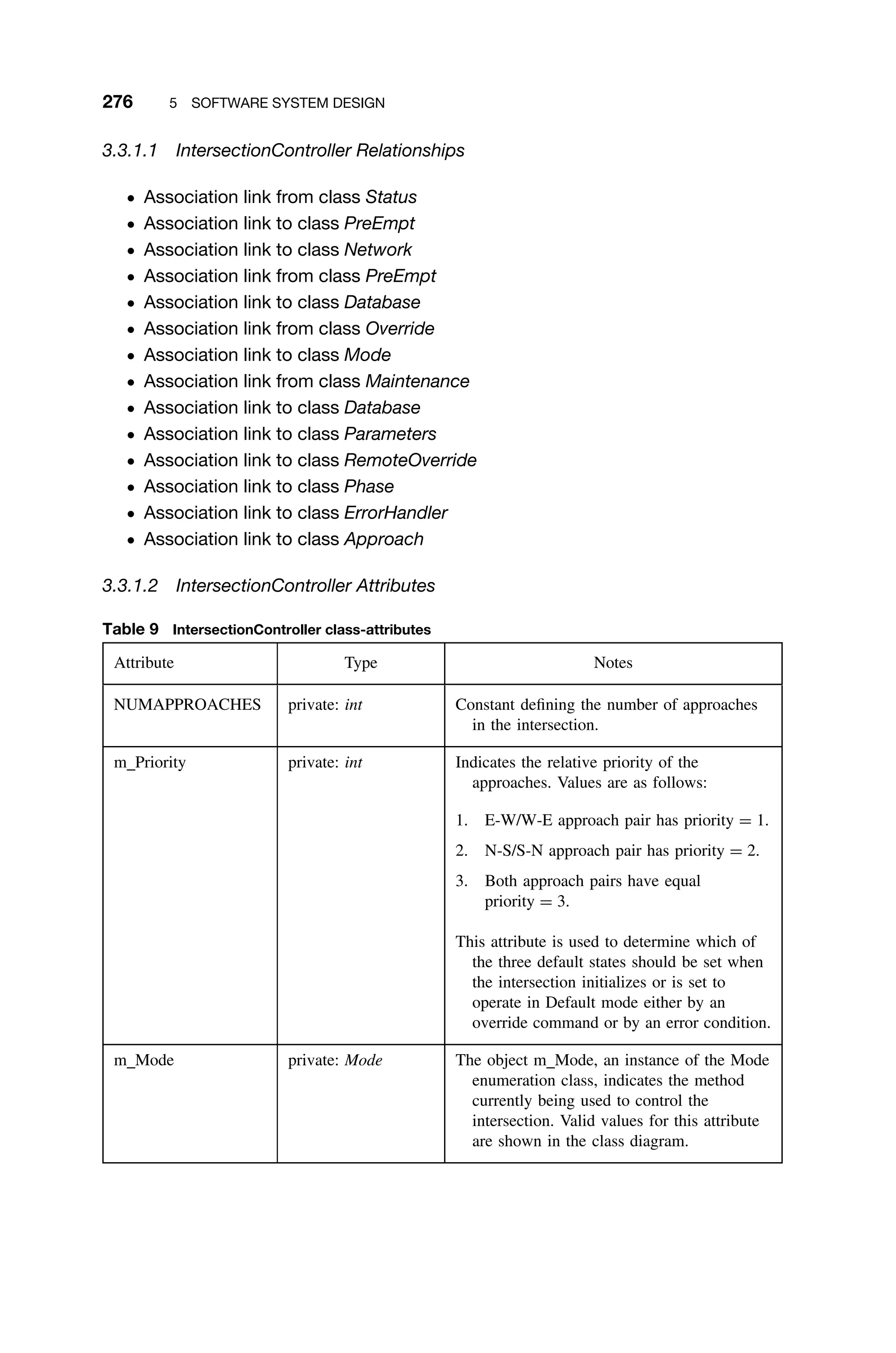
![5.6 APPENDIX: CASE STUDY IN SOFTWARE REQUIREMENTS SPECIFICATION 277
Table 9 (continued)
Attribute Type Notes
The setPhase() method checks for changes in
this value at the beginning of each cycle
and changes the control scheme if required.
Changes to Preempt, Manual or Remote
modes are handled by specific events; these
events cause the control scheme to change
immediately rather than at the beginning of
the next cycle.
m CurrentPhase private: Phase This is an enumeration of class Phase that
also serves as an index into the m Split
array (since C++ automatically casts
enumerated types as arrays where required)
denoting which portion of the cycle is
currently active.
The Default phase is used during initialization
and in response to override commands and
critical system faults. Phases
GG GG RR RR (1) to RR RR RR RR 8
(8) are used in normal operation.
m ErrorHandler private:
ErrorHandler
Pointer to the m ErrorHandler object.
m Approach private: Approach This is an array of type Approach and a
length of NUMAPPROACHES. This array
represents each of the four entrances to an
intersection. See the Approach class for
more details.
The m Approach array is declared as follows:
Approach
m Approach[NUMAPPROACHES]
Where NUMAPPROACHES is a
compile-time constant.
m Network private: Network This object is the instance of the Network
class that provides an abstraction layer
between the network resource manager and
the m IntersectionController object.
m EmergencyPreempt private: PreEmpt This is a pointer to the instance of the
PreEmpt class that provides an abstraction
layer between the emergency vehicle
transponder resource manager and the
m IntersectionController object.
(continued)](https://image.slidesharecdn.com/epdf-230618090952-bdcb6616/75/epdf-pub_real-time-systems-design-and-analysis-pdf-300-2048.jpg)
![278 5 SOFTWARE SYSTEM DESIGN
Table 9 (continued)
Attribute Type Notes
m Parameters private: Parameters Structure holding the intersection parameters,
which are the cycle time and the splits
array.
m RemoteOverride private:
RemoteOverride
This is the instance of the RemoteOverride
class representing the Remote Software
console. This object abstracts requests
made from the off-site software control
panel from the main application.
m ManualOverride private: Override This is the instance of the Override class
representing the Manual Override console.
The object serves as a broker, abstracting
the main application from any requests
made from the Manual Override console,
which is located at the site of the traffic
control system.
m LocalTimeZone private: float Given as an offset in hours to UTC (GMT).
m TrafficHistory private: Database This is the instance of the Database class that
is used to log statistical data regarding
traffic levels at the intersection being
controlled. The data are stored in the
system’s flash memory store. See
Section 2.2.6.1 in [1] for more information
about the flash memory included in the
system.
m IncidentLog private: Database This object, which is another instance of the
Database class, logs abnormal events
observed by the system on the site of the
intersection. Data recorded by this object
will be stored in the system’s flash memory
store. See Section 2.2.6.1 in [1] for more
information about the flash memory
included in the system.
m Aspect private: Aspect Detected Aspect from each m Approach
object; Aspect[4].
m Count private: int Vehicle count from each m Approach object;
int[4].
m IntersectionStatus private: Status](https://image.slidesharecdn.com/epdf-230618090952-bdcb6616/75/epdf-pub_real-time-systems-design-and-analysis-pdf-301-2048.jpg)
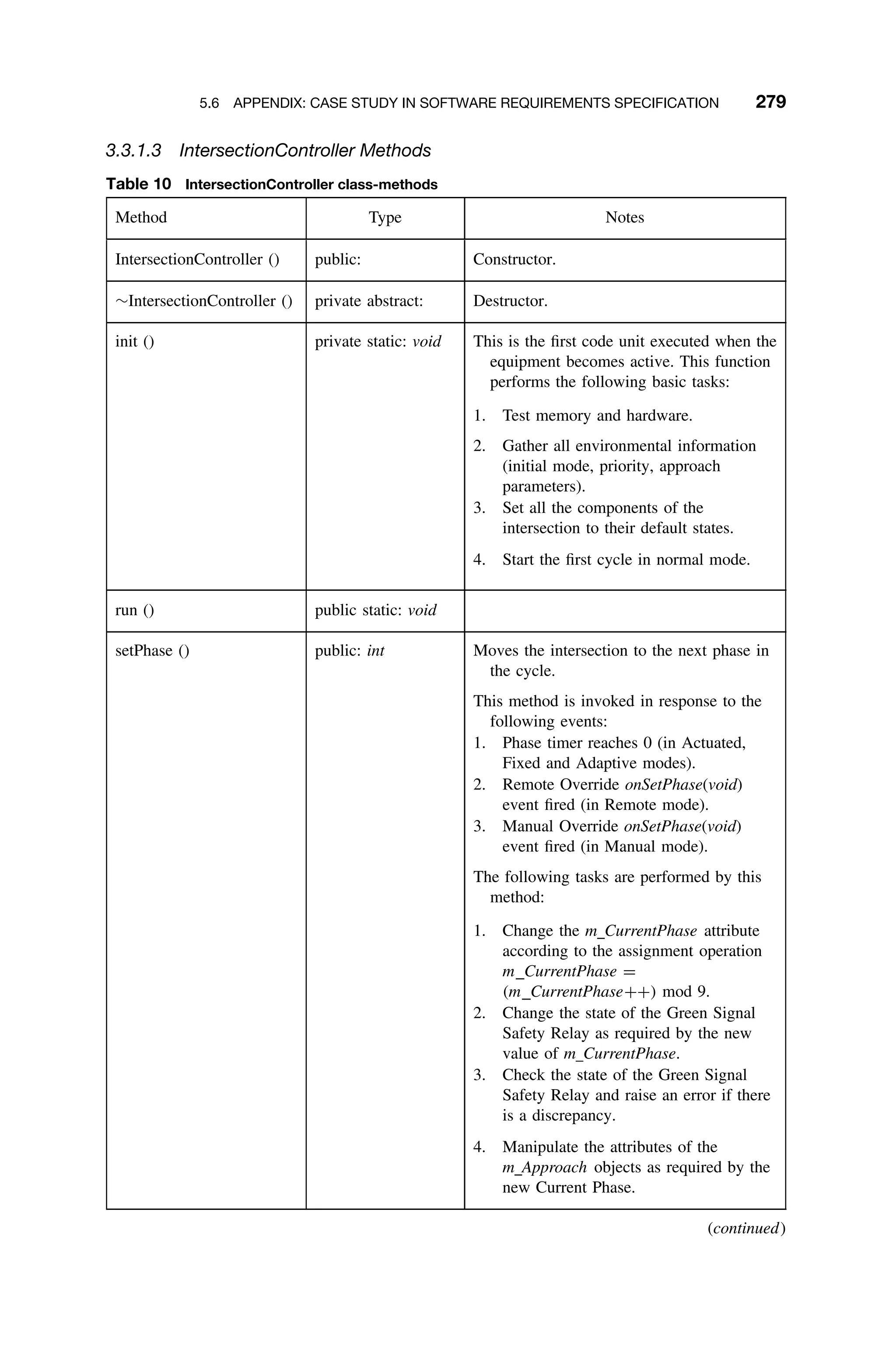
![280 5 SOFTWARE SYSTEM DESIGN
Table 10 (continued)
Method Type Notes
5. Calculate the phase time as
calculateTime(m Cycle,
m Splits[m CurrentPhase]).
6. Load the Phase Time Remaining timer
with the calculated phase time by
invoking
loadTimer(calculateTime(m Cycle,
m Splits[m CurrentPhase])).
7. Check that the phase setting is
displayed properly by the approaches
and raise an error if there is a
discrepancy.
setPhase (Phase) public: int param: phase [Phase - in]
Moves the intersection to the specified
phase.
getPhase () public: Phase Determine the displayed intersection phase
by querying all Aspect objects and
determining their aspects. Used by the
checkPhase method
checkPhase (Phase) public: boolean param: phase [Phase - in]
Returns True if the displayed phase agrees
with the commanded phase (passed as a
parameter), False otherwise.
setCycle (float) public: int param: time [float - in]
Mutator for the cycle time attribute.
getCycle () public: float Accessor for the cycle time attribute.
setSplits (Split∗
) public: int param: splits [Split∗
- inout]
Mutator for the splits attribute.
getSplits () public: Split∗
Accessor for the splits attribute.
setMode (Mode) public: int param: mode [Mode - in]
Mutator for the attribute m Mode.
getMode () public: Mode Accessor for the attribute m Mode.
checkMode (Mode) public: boolean param: mode [Mode - in]](https://image.slidesharecdn.com/epdf-230618090952-bdcb6616/75/epdf-pub_real-time-systems-design-and-analysis-pdf-303-2048.jpg)
![5.6 APPENDIX: CASE STUDY IN SOFTWARE REQUIREMENTS SPECIFICATION 281
Table 10 (continued)
Method Type Notes
loadTimer (float) public: int param: time [float - in]
Loads the phase timer (utilizing OS timer
services) with the phase time, specified as
a parameter.
onPreemptRequest () public: int Emergency preempt request event from the
m EmergencyPreempt object. This
method performs the following tasks:
1. Save the current value of m Mode.
2. Set the mode to Preempt.
3. Set the intersection phase to allow the
emergency vehicle to pass safely under
traffic signal control.
onPreemptCleared () public: int Event that terminates preempted operation
and returns the intersection to normal
operating mode. This method performs
the following tasks:
1. Restores the previous mode.
2. Sets the intersection to the default state.
3. Returns the intersection to normal
operation.
onOverrideActivated
(OverrideType)
public: int param: type [OverrideType - in]
Override activation event from either the
m ManualOverride or m RemoteOverride
object. The parameter type indicates
which override is involved. This method
performs the following tasks:
1. Save the current value of m Mode.
2. Set the mode to Manual or Remote,
depending on the value of parameter
type.
3. Set the intersection to the Default
phase.
onOverrideDeactivated
(OverrideType)
public: int param: type [OverrideType - in]
(continued)](https://image.slidesharecdn.com/epdf-230618090952-bdcb6616/75/epdf-pub_real-time-systems-design-and-analysis-pdf-304-2048.jpg)
![282 5 SOFTWARE SYSTEM DESIGN
Table 10 (continued)
Method Type Notes
Override cancellation event from either the
m ManualOverride or m RemoteOverride
object. The parameter type indicates
which override is involved. This method
performs the following tasks:
1. Restore the previous value of m Mode.
2. Set the intersection to the Default
phase.
3. Returns the intersection to normal
operation.
toggleGreenSafetyRelay () public: int Toggles the state of the Green Safety Relay.
checkGreenSafetyRelay () public: boolean Checks that the Green Safety Relay is in the
proper state for the active intersection
phase.
calculateParameters () public: int Adaptive algorithm for determining
intersection timing parameters for the
next cycle.
calculateTime (float,
Split∗
)
public: float param: cycle [float - in]
param: split [Split∗
- in]
Used to calculate the actual phase time from
the values of m Parameters.cycleTime
and m Parameters.splits.
setParameters () public: int Mutator for the intersection timing
parameters.
getParameters () public: Parameters∗
Accessor for the intersection timing
parameters.
getStatus () public: Status∗
Method used to access the overall status of
the intersection.
onPedestrianRequest () public: void Event triggered by a valid pedestrian
crossing request.
onVehicleEntry (int) public: void param: approach [int - in]
Event triggered by a vehicle entering the
vehicle detection loop.](https://image.slidesharecdn.com/epdf-230618090952-bdcb6616/75/epdf-pub_real-time-systems-design-and-analysis-pdf-305-2048.jpg)
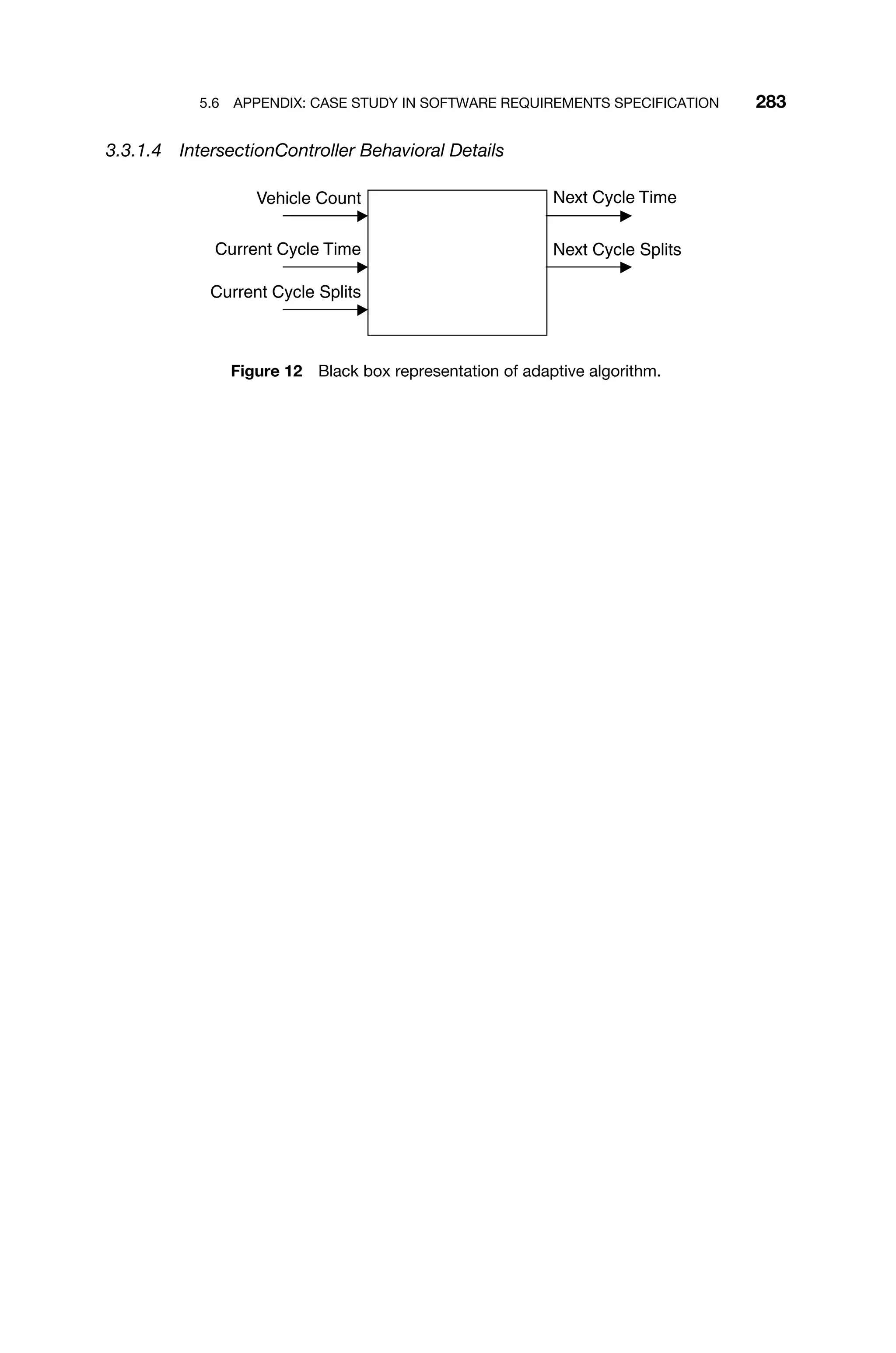
![284 5 SOFTWARE SYSTEM DESIGN
{While Running}
singleton
m_IntersectionController
:IntersectionController
m_Approach[i]
:Approach
m_PedestrianTrafficStandard[j]
:IntersectionStandard
m_VehicleTrafficStandard[k]
:IntersectionStandard
Name: IntersectionController- Traffic Signal Control
Author: Team 2
Version: 1.0
Created: 08-Dec-2002 14:25:38
Updated: 09-Dec-2002 13:54:53
{t0 = 0}
init()
Approach()
IntersectionStandard()
IntersectionStandard()
m_Status: = setPhase(phase)
init complete
{t0 = 5 s}
run()
{t1 = 0}
m_Status: = setPhase()
setAspect(aspect)
setIndication(indication)
{t1 = 100 ms}
*m_CurrentIndication = indication
setIndication(indication)
{t1 = 100 ms}
m_CurrentIndication = indication
{t1 = 50 ms}
m_Status: = return value
loadTimer(time)
{t1 = 100 ms}
[m_CurrentPhase = = 4 || m_CurrentPhase = = 8]:toggleGreenSafetyRelay()
checkPhase(phase)
{t1 = 120 ms}
getAspect()
m_Indication: = getIndication()
m_Indication: = getIndication()
{t1 = 220 ms}
m_Aspect: = return value
{t1 = 230 ms}
m_Status: = return value
{t1 = 240 ms}
{t1 = 300 ms}
[m_CurrentPhase = = 8]:calculateParameters()
*[While Phase Timer 0]:idle
(Keep-Alive Pseudo-Message)
(Keep-Alive Pseudo-Message)
(Keep-Alive Pseudo-Message)
m_Status: = checkGreenSafetyRelay()
Figure 13 Traffic signal control sequence diagram.](https://image.slidesharecdn.com/epdf-230618090952-bdcb6616/75/epdf-pub_real-time-systems-design-and-analysis-pdf-307-2048.jpg)
![5.6 APPENDIX: CASE STUDY IN SOFTWARE REQUIREMENTS SPECIFICATION 285
Running
Phase RR-RR-RR-RR
Phase GG-GG-RR-RR
+ Do Action / setPhase(void)
+ Do Action / loadTimer(Phase 1 Time)
+ Do Action / checkPhase(Phase 1)
Phase GY-GY-RR-RR
+ Do Action / setPhase(void)
+ Do Action / loadTimer(Phase 2 Time)
+ Do Action / checkPhase(Phase 2)
Phase YR-YR-RR-RR
+ Do Action / setPhase(void)
+ Do Action / loadTimer(Phase 3 Time)
+ Do Action / checkPhase(Phase 3)
Phase RR-RR-GG-GG
+ Do Action / setPhase(void)
+ Do Action / loadTimer(Phase 5 Time)
+ Do Action / checkPhase(Phase 5)
Phase RR-RR-GY-GY
+ Do Action / setPhase(void)
+ Do Action / loadTimer(Phase 6 Time)
+ Do Action / checkPhase(Phase 6)
Phase RR-RR-YR-YR
+ Do Action / setPhase(void)
+ Do Action / loadTimer(Phase 7 Time)
+ Do Action / checkPhase(Phase 7)
See diagram
for this state
Name: IntersectionController- Running
Author: Team 2
Version: 1.0
Created: 16-Nov-2002 17:12:04
Updated: 05-Dec-2002 19:49:42
phaseTimerExpired 1 phaseTimerExpired 2
phaseTimerExpired 3 /lastPhase = FALSE
phaseTimerExpired 4
phaseTimerExpired 5
phaseTimerExpired 6
phaseTimerExpired 7 /lastPhase = TRUE
phaseTimerExpired 8
Figure 14 Statechart for intersectionController phase sequence.
Phase RR-RR-RR-RR
Start
Setting Phase 4
+ Do Action / setPhase(Phase 4)
+ Do Action / loadTimer(Phase 4 Time)
+ Do Action / checkPhase
Setting Phase 8
+ Do Action / setPhase(Phase 8)
+ Do Action / loadTimer(Phase 8 Time)
+ Do Action / checkPhase
Preparing for Next Cycle
+ Do Action / calculateParameters
Toggling Green Safety Relay
+ Do Action / toggleGreenSafetyRelay
+ Do Action / checkGreenSafetyRelay
Name: Intersection Controller- Phase RR-RR-RR-RR
Author: Team 2
Version: 1.0
Created: 17-Nov-2002 19:22:39
Updated: 30-Nov-2002 17:56:13
Pedestrian requests are not
shown in this diagram.
Phase Timer Expired H
Phase Timer Expired C
[lastPhase = = TRUE]
[lastPhase = = FALSE]
Figure 15 Statechart for Phases 4 and 8.](https://image.slidesharecdn.com/epdf-230618090952-bdcb6616/75/epdf-pub_real-time-systems-design-and-analysis-pdf-308-2048.jpg)
![286 5 SOFTWARE SYSTEM DESIGN
3.3.2 Approach This is the programmatic representation of an individual entrance
into the intersection.
The Approach class is responsible for managing the following functions:
1. Instantiation of contained objects.
2. Control of the traffic standards associated with the approach.
3. Handling of pedestrian crossing events.
4. Handling of loop detector entry and exit events.
5. Tracking the vehicle count.
Figure 16 illustrates the attributes, methods, and events of the Approach class.
Approach
{4}
− m_CurrentAspect: Aspect
− m_PedestrianDetector: OnOffSensor* [2 ordered]
− m_VehicleDetector: VehicleDetector*
− m_VehicleTrafficStandard: IntersectionStandard* [2 ordered]
− m_PedestrianTrafficStandard: IntersectionStandard* [2 ordered]
− m_Indication: Indication* [4 ordered]
− m_Count: int
− m_SpeedLimit: int
+ Approach()
−* ∼Approach()
+ setAspect(Aspect) : void
+ getAspect() : Aspect*
+ getCount() : int*
+ bumpCount(void) : void
+ clearCount(void) : void
+ onPedestrianRequest() : void
+ onEntryStateSet(void) : void
+ onEntryStateCleared(void) : void
Figure 16 Approach class.
3.3.2.1 Aspect Relationships
ž Association link to class IntersectionStandard
ž Association link to class Aspect
ž Association link to class IntersectionStandard
ž Association link to class VehicleDetector
ž Association link to class OnOffSensor
ž Association link from class IntersectionController](https://image.slidesharecdn.com/epdf-230618090952-bdcb6616/75/epdf-pub_real-time-systems-design-and-analysis-pdf-309-2048.jpg)
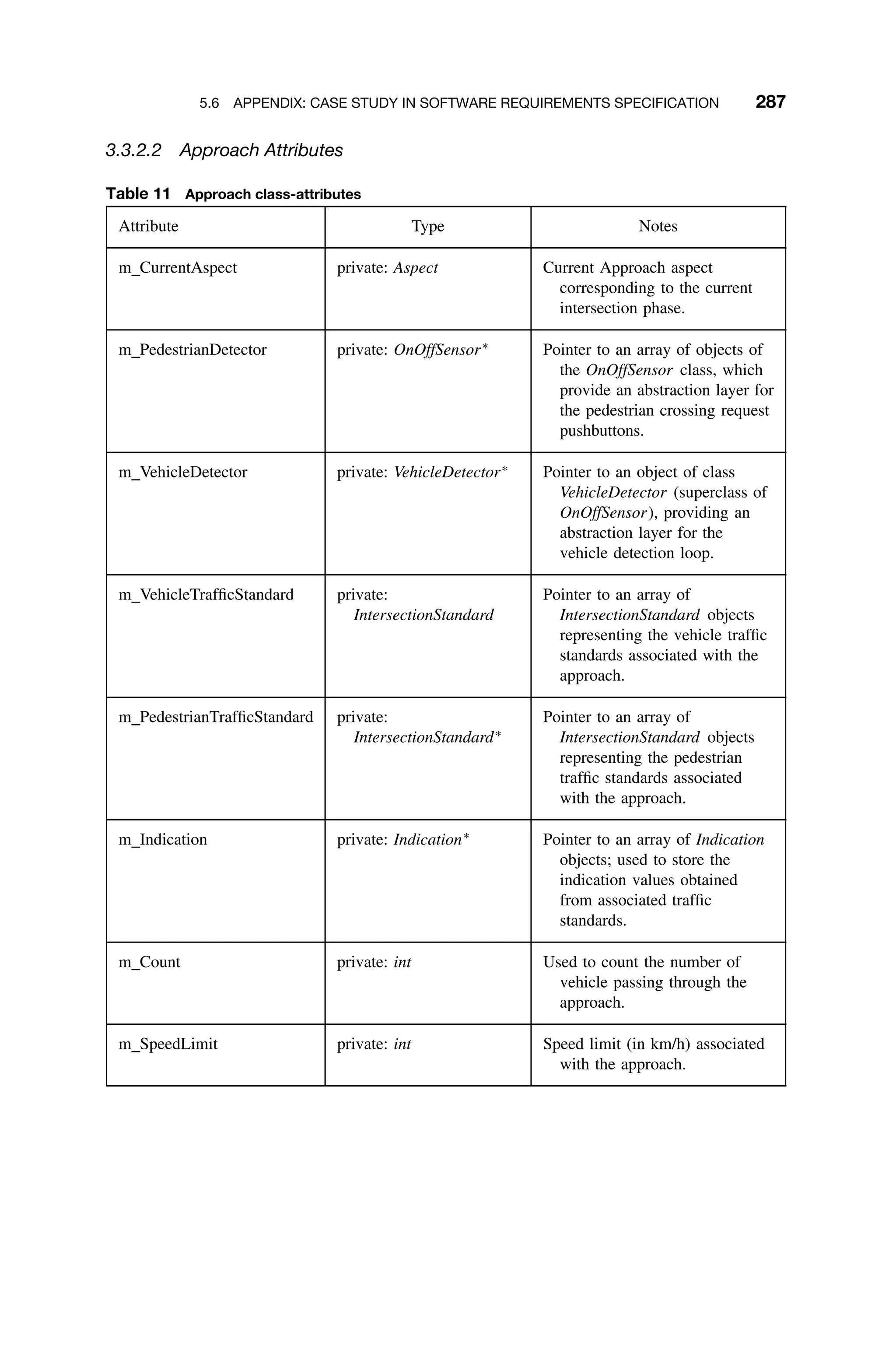
![288 5 SOFTWARE SYSTEM DESIGN
3.3.2.3 Approach Methods
Table 12 Approach class-methods
Method Type Notes
Approach () public: Constructor.
∼Approach () private abstract: Destructor.
setAspect (Aspect) public: void param: aspect [Aspect - in]
Mutator for attribute m CurrentAspect.
getAspect () public: Aspect∗
Accessor used to fetch the aspect actually
being displayed by the set of approach
traffic standards.
getCount () public: int∗
Accessor for the m Count attribute.
bumpCount (void) public: void Method called to increment the attribute
m Count by 1.
clearCount (void) public: void Method called to set the attribute m Count
to 0.
onPedestrianRequest () public: void Event triggered by a valid pedestrian
crossing request from one of the
pedestrian request pushbuttons
associated with the approach.
onEntryStateSet (void) public: void Event triggered when the vehicle detector
attribute m State is set.
onEntryStateCleared (void) public: void Event triggered when the vehicle detector
attribute m State is cleared.
3.3.3 IntersectionStandardClass(PedestrianTrafficVehicleTrafficStandard)
This is the programmatic representation of a traffic control signal.
The IntersectionStandard class is responsible for managing the following functions:
1. Displaying the commanded aspect from the Intersection Controller.
2. Determining the aspect actually displayed.
3. Checking for discrepancies between commanded and displayed aspects.
4. Raising an error event if there is an aspect discrepancy.
Figure 17 illustrates the attributes, methods, and events of the IntersectionStan-
dard class.](https://image.slidesharecdn.com/epdf-230618090952-bdcb6616/75/epdf-pub_real-time-systems-design-and-analysis-pdf-311-2048.jpg)
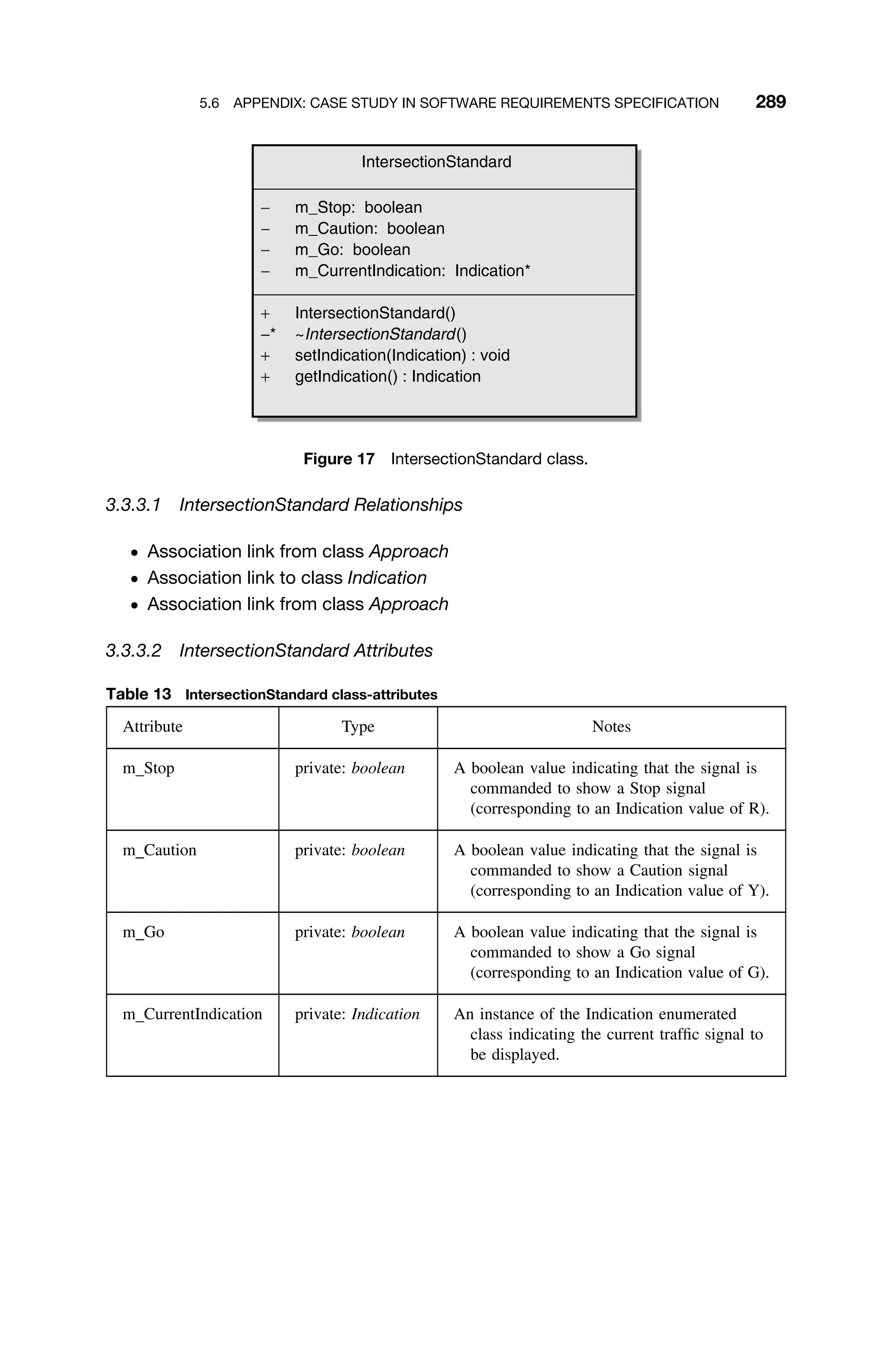
![290 5 SOFTWARE SYSTEM DESIGN
3.3.3.3 IntersectionStandard Methods
Table 14 IntersectionStandard class-methods
Method Type Notes
IntersectionStandard () public: Constructor.
∼IntersectionStandard () private abstract: Destructor.
setIndication (Indication) public: void param: indication [Indication - in]
Mutator for the m CurrentIndication attribute.
The method performs the following:
1. Check whether the commanded aspect
is valid. If not, raise an error.
2. If the commanded aspect is valid,
display it.
getIndication () public: Indication Accessor for determining the value of the
indication actually being displayed.
3.3.3.4 Correspondence between Indications and Actual Displayed Signals Since
this class is used for both the Vehicle and Pedestrian Traffic Standard objects, it
is necessary to define the relationship between the attribute values and the actual
displayed signal; this is shown in Table 15.
Table 15 Attribute and signal correspondence
m CurrentIndication m Stop m Caution m Go Vehicle
Standard
Pedestrian
Standard
R True False False Red DON’T WALK
Y False True False Amber Flashing DON’T WALK
G False False True Green WALK
3.3.4 OnOffSensor This class represents the pedestrian crossing request push-
buttons located on opposite sides of the crosswalk associated with an approach.
Objects of the OnOffSensor class are responsible for managing the follow-
ing functions:
1. Filtering of pushbutton service requests.
2. Generation of Pedestrian Service Request event.
Figure 18 illustrates the attributes, methods, and events of the OnOffSensor class.](https://image.slidesharecdn.com/epdf-230618090952-bdcb6616/75/epdf-pub_real-time-systems-design-and-analysis-pdf-313-2048.jpg)
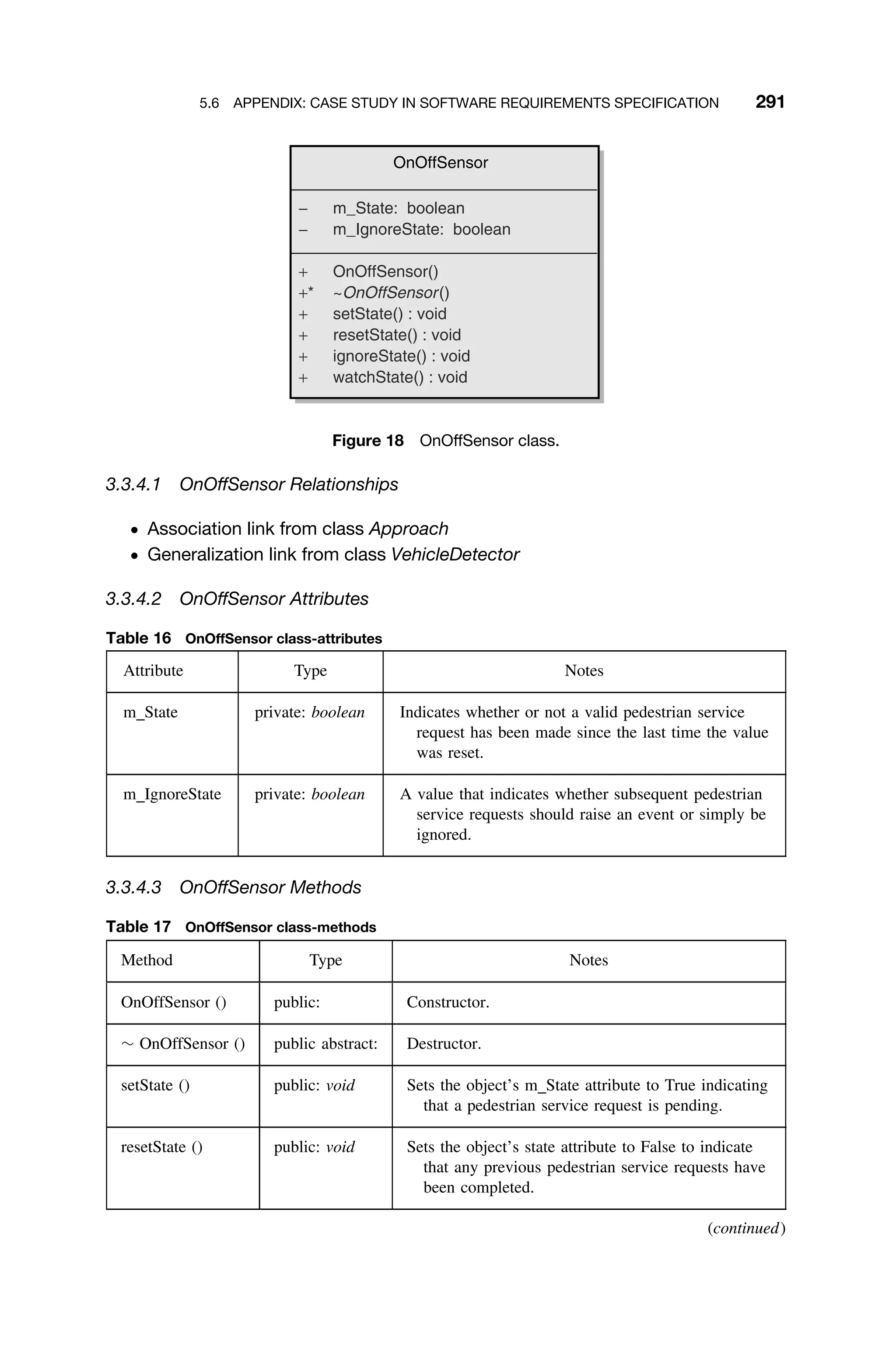
![292 5 SOFTWARE SYSTEM DESIGN
Table 17 (continued)
Method Type Notes
ignoreState () public: void Sets the object’s m IgnoreState attribute to True
indicating that subsequent pedestrian requests are
to be ignored.
watchState () public: void Sets the object’s m IgnoreState attribute to False
indicating that subsequent pedestrian requests are
to be processed.
3.3.4.4 OnOffSensor Behavioral Details
«singleton»
m_IntersectionController
:IntersectionController
m_PedestrianDetector[j]
:OnOffSensor
m_Approach[i]
:Approach
Name: IntersectionController- Pedestrian Request
Author: Team 2
Version: 1.0
Created: 09-Dec-2002 12:15:35
Updated: 09-Dec-2002 14:05:38
{t0 = 0}
m_State = True
{t0 = 50 ms}
onPedestrianRequest()
{t0 = 100 ms}
onPedestrianRequest()
{t1 = 0}
setPhase()
setAspect(aspect)
resetState()
{t1 = 100 ms}
m_State = False
Figure 19 OnOffSensor sequence diagram.](https://image.slidesharecdn.com/epdf-230618090952-bdcb6616/75/epdf-pub_real-time-systems-design-and-analysis-pdf-315-2048.jpg)
![5.6 APPENDIX: CASE STUDY IN SOFTWARE REQUIREMENTS SPECIFICATION 293
Pedestrian Detector- Operation
Processing Request
Waiting for Pedestrian Request
Waiting for
Positive-Going
Transition
Waiting for
Negative-Going
Transition
Receiving Request
Setting Ignore State
+ Do Action / m_IgnoreState = True
Setting Request State
+ Do Action / m_State = True
Clearing Request State
+ Do Action / m_State = False
m_Approach[i]
:Approach
Clearing Ignore State
+ Do Action / m_IgnoreState = False
No Transition No Transition
/watchState()
[m_IgnoreState == False] /setState()
/ignoreState()
/onPedestrianRequest()
/resetState()
Positive-Going Transition
Negative-Going
Transition
[m_IgnoreState == True]
Figure 20 OnOffSensor statechart.](https://image.slidesharecdn.com/epdf-230618090952-bdcb6616/75/epdf-pub_real-time-systems-design-and-analysis-pdf-316-2048.jpg)
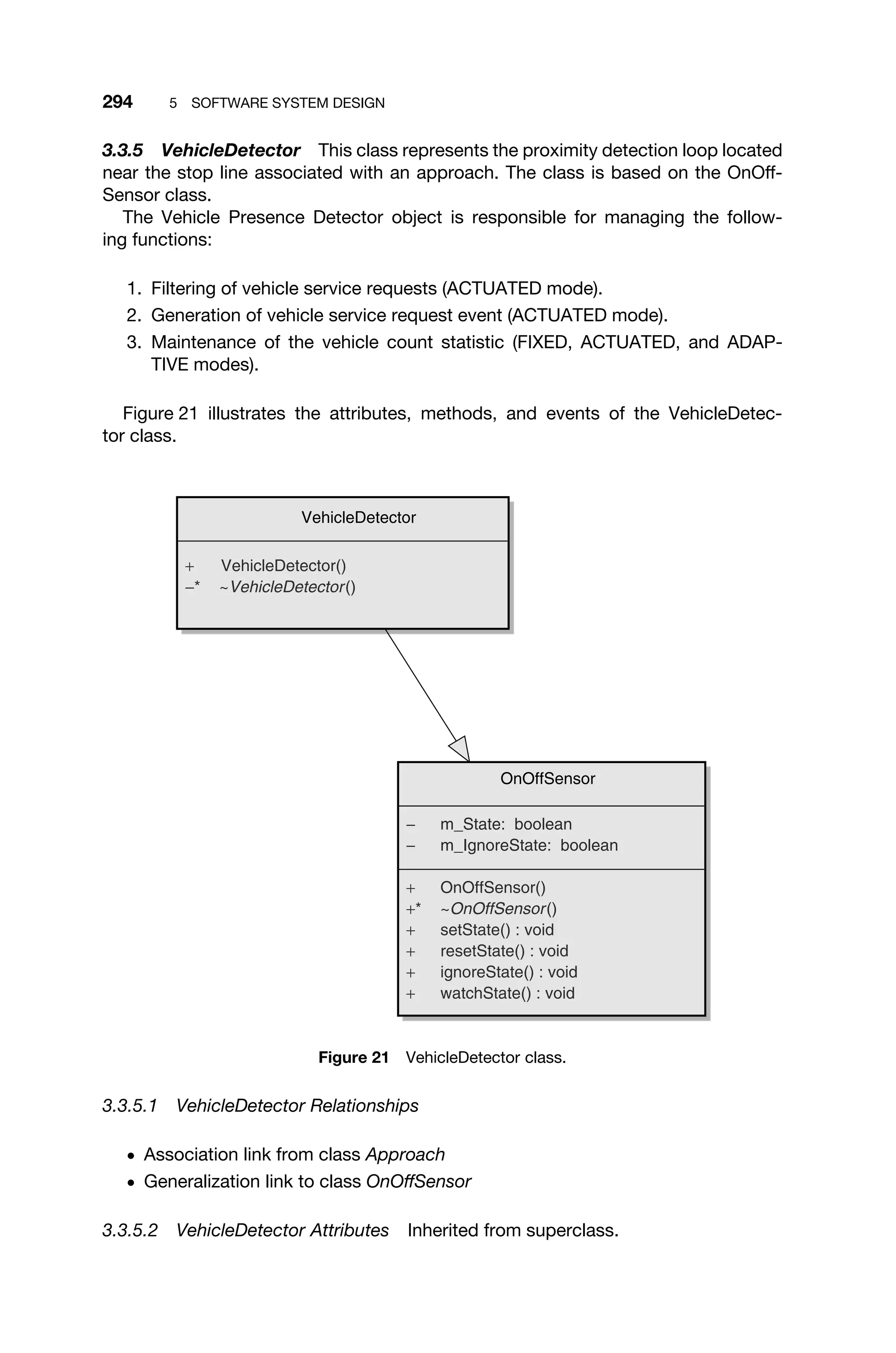
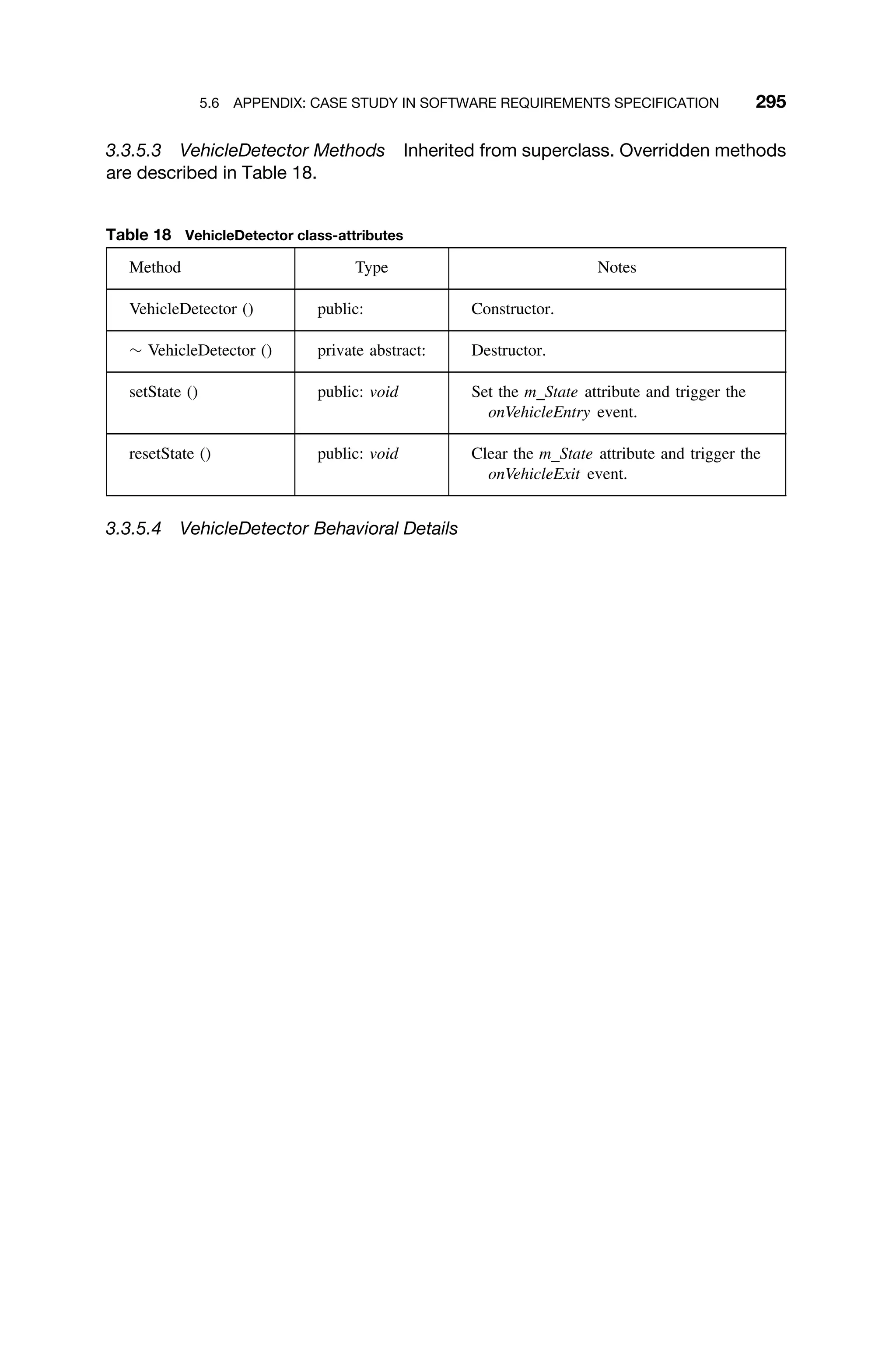
![296 5 SOFTWARE SYSTEM DESIGN
m_Approach[i].m_VehicleDetector
:VehicleDetector
m_Approach[i]
:Approach
«singleton»
m_IntersectionController
:IntersectionController
Name:
IntersectionController-
Vehicle
Detector
Author:
Team
2
Version:
1.0
Created:
07-Dec-2002
21:54:19
Updated:
09-Dec-2002
13:58:06
{t1
=
0}
*[While
Approach
Aspect
=
=
{G,Y]*]:onEntryStateSet(void)
{t1
=
50
ms}
onVehicleEntry(approach)
{t2
=
0}
*[While
Approach
Aspect
=
=
[G,Y]*]:onEntryStateCleared(void)
{t2
=
20
ms}
m_Count++
{t3
=
0}
[if
(Approach
Aspect
Changes
to
RR)]:clearCount(void)
{t3
=
20
ms}
m_Count
=
0
Figure
22
VehicleDetector
class
sequence
diagram.](https://image.slidesharecdn.com/epdf-230618090952-bdcb6616/75/epdf-pub_real-time-systems-design-and-analysis-pdf-319-2048.jpg)
![5.6 APPENDIX: CASE STUDY IN SOFTWARE REQUIREMENTS SPECIFICATION 297
Intersection Controller-Operating
m_VehicleDetector[i]
Blocked
Vehicle Over Loop
+ Do Action / setState(void)
+ Do Action / m_Approach[i].onEntryStateSet(void)
Vehicle Has Passed Loop
+ Do Action / resetState(void)
+ Do Action / m_Approach[i].onEntryStateCleared(void)
m_Approach[i]
Updating Count
+ Do Action / m_Count++
Blocked
Triggering Approach
+ Do Action / m_IntersectionController.onVehicleEntry(int)
Clearing Count
+ Do Action / m_Count = 0
Name: IntersectionController- Vehicle Detector
Author: Team 2
Version: 1.0
Created: 06-Dec-2002 15:21:47
Updated: 07-Dec-2002 21:46:52
Vehicle Entry
Vehicle Exit
onEntryStateCleared
onEntryStateSet
clearCount()
Figure 23 VehicleDetector class statechart.
3.3.6 Override This is class represents the set of pushbuttons on the manual
override console.](https://image.slidesharecdn.com/epdf-230618090952-bdcb6616/75/epdf-pub_real-time-systems-design-and-analysis-pdf-320-2048.jpg)
![298 5 SOFTWARE SYSTEM DESIGN
Override
− m_IntersectionController: IntersectionController*
+ Override()
−* ~Override()
+ onActivate(OverrideType) : int
+ onDeactivate(OverrideType) : int
+ onSetPhase() : int
Figure 24 Override class.
3.3.6.1 Override Relationships
ž Dependency link to class OverrideType
ž Association link to class IntersectionController
ž Generalization link from class RemoteOverride
3.3.6.2 Override Attributes
Table 19 Override class-attributes
Attribute Type Notes
m IntersectionController private:
IntersectionController
Pointer to the
m IntersectionController
object.
3.3.6.3 Override Methods
Table 20 Override class-methods
Method Type Notes
Override () public: Constructor.
∼ Override () private abstract: Destructor.
onActivate
(OverrideType)
public: int param: type [OverrideType - in]
Event triggered by receipt of an activation
command from the local override console.
onDeactivate
(OverrideType)
public: int param: type [OverrideType - in]
Event triggered by receipt of an deactivation
command from the local override console.
onSetPhase () public: int Event triggered by receipt of an advance
phase command from the local override
console.](https://image.slidesharecdn.com/epdf-230618090952-bdcb6616/75/epdf-pub_real-time-systems-design-and-analysis-pdf-321-2048.jpg)
![5.6 APPENDIX: CASE STUDY IN SOFTWARE REQUIREMENTS SPECIFICATION 299
3.3.6.4 Override Behavioral Details
m_ManualOverride
:Override
«singleton»
m_IntersectionController
:IntersectionController
«resource»
:Manual
Control Panel
Name: IntersectionController- Manual Override
Author: Team 2
Version: 1.0
Created: 04-Dec-2002 08:30:25
Updated: 05-Dec-2002 18:52:22
{t0 = 0}
dispatchCommand(command = Activate Manual Override)
{t0 = 10 ms}
onActivate(type)
{t0 = 20 ms}
onOverrideActivated(type)
m_PreviousMode = m_Mode
m_Mode = Manual
setPhase(phase = Default)
checkPhase(phase)
{t0 = 220 ms}
m_Status:= 0 (OK)
{t0 = 250 ms}
m_Status:= 0 (OK)
{t1 = 0}
*[While Override Active]:dispatchCommand(command = Advance Phase)
{t1 = 10 ms}
{t1 = 20 ms}
*[While Override Active]:setPhase()
setPhase()
checkPhase(phase)
{t1 = 220 ms}
*[While Override Active]: m_Status:= 0 (OK)
{t1 = 250 ms}
*[While Override Active]: m_Status:= 0 (OK)
{t2 = 0}
dispatchCommand(command = Deactivate Manual Override)
{t2 = 10 ms}
onDeactivate(type)
{t2 = 20 ms}
onOverrideDeactivated(type)
m_Mode = m_PreviousMode
setPhase(phase)
checkPhase(phase)
{t2 = 220 ms}
m_Status:= 0 (OK)
{t2 = 250 ms}
m_Status:= 0 (OK)
*[While Override Active]:onSetPhase()
Figure 25 Override class sequence diagram.](https://image.slidesharecdn.com/epdf-230618090952-bdcb6616/75/epdf-pub_real-time-systems-design-and-analysis-pdf-322-2048.jpg)
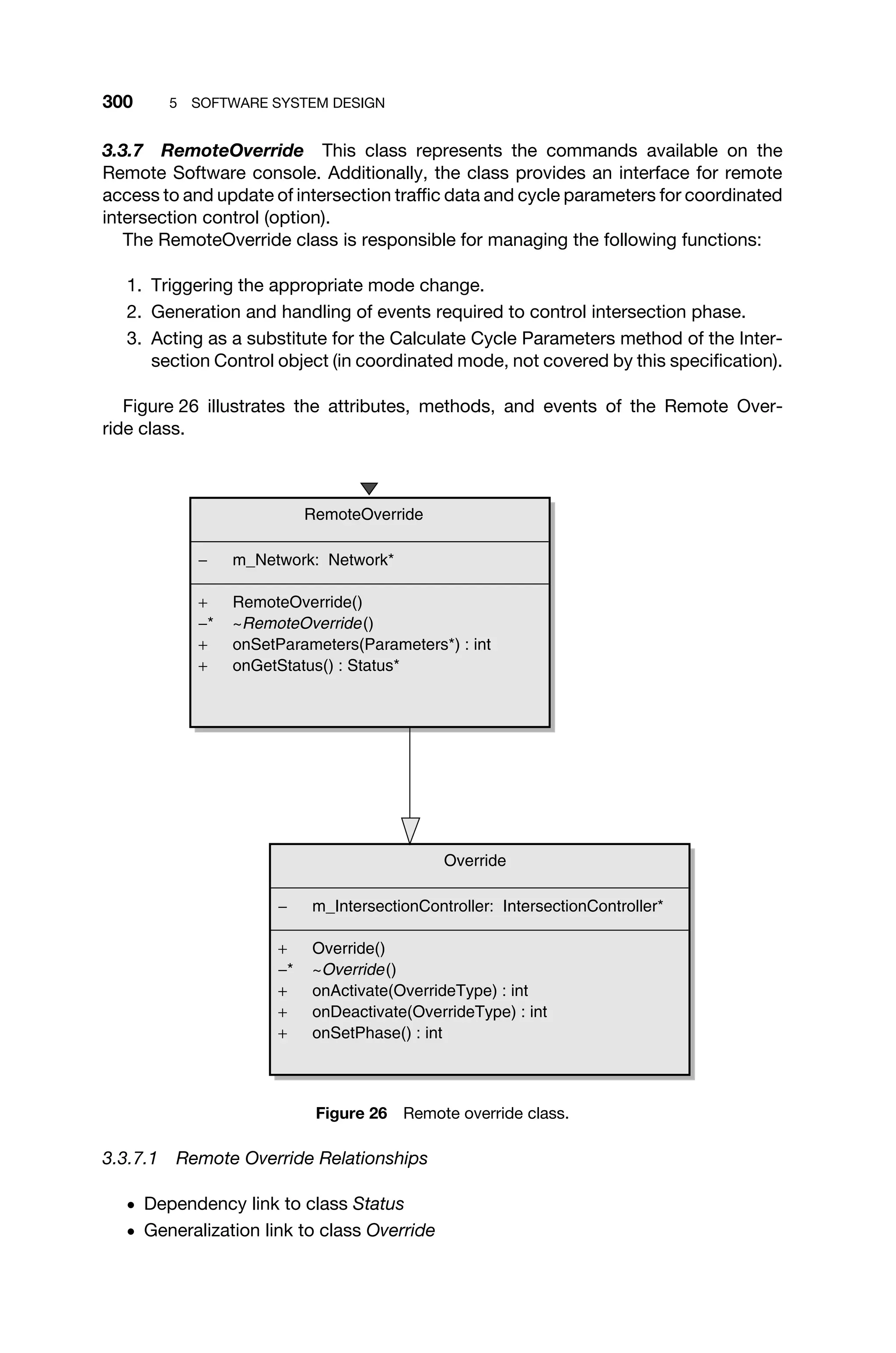
![5.6 APPENDIX: CASE STUDY IN SOFTWARE REQUIREMENTS SPECIFICATION 301
ž Association link from class IntersectionController
ž Association link to class Network
3.3.7.2 RemoteOverride Attributes In addition to those inherited from the super-
class Override, RemoteOverride attributes are as listed in Table 21.
Table 21 RemoteOverride class-attributes
Attribute Type Notes
m Network private: Network Pointer to the m Network object.
3.3.7.3 RemoteOverride Methods In addition to those inherited from the super-
class Override, RemoteOverride methods are as listed in Table 22.
Table 22 RemoteOverride class-methods
Method Type Notes
RemoteOverride () public: Constructor.
∼ RemoteOverride () private abstract: Destructor.
onSetParameters
(Parameters∗
)
public: int param: parameters [Parameters∗
- in]
Event triggered under coordinated control; used
to set the intersection timing parameters under
remote control.
Completes within 100 ms.
onGetStatus () public: Status∗
Event triggered under coordinated control; used
to get the intersection timing parameters under
remote control.
Completes within 100 ms.
3.3.7.4 RemoteOverride Behavioral Details Behavior of the RemoteOverride class
is identical to that of the Override class for methods inherited from the superclass.
3.3.8 PreEmpt This class manages the wireless transponder interface to autho-
rized emergency vehicles and accesses the m IntersectionControl object in order to
display the correct traffic signals, allowing the emergency vehicle priority access to
the intersection.
The PreEmpt class is responsible for managing the following functions:
1. Triggering the appropriate mode change.
2. Reception of emergency vehicle preemption requests.
3. Decryption and validation of emergency vehicle preemption requests.
4. Generation and handling of events required to control intersection phase.](https://image.slidesharecdn.com/epdf-230618090952-bdcb6616/75/epdf-pub_real-time-systems-design-and-analysis-pdf-324-2048.jpg)
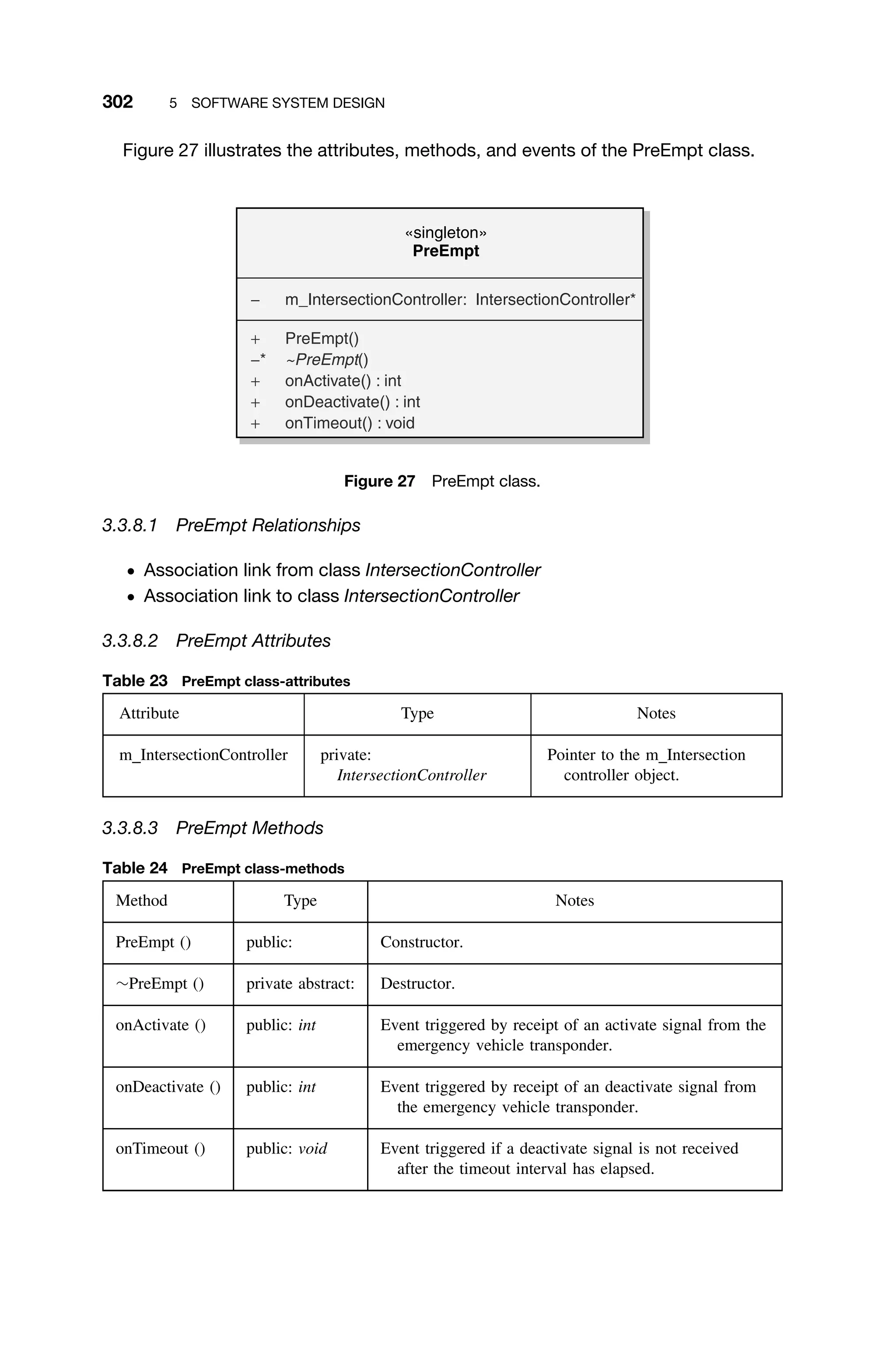
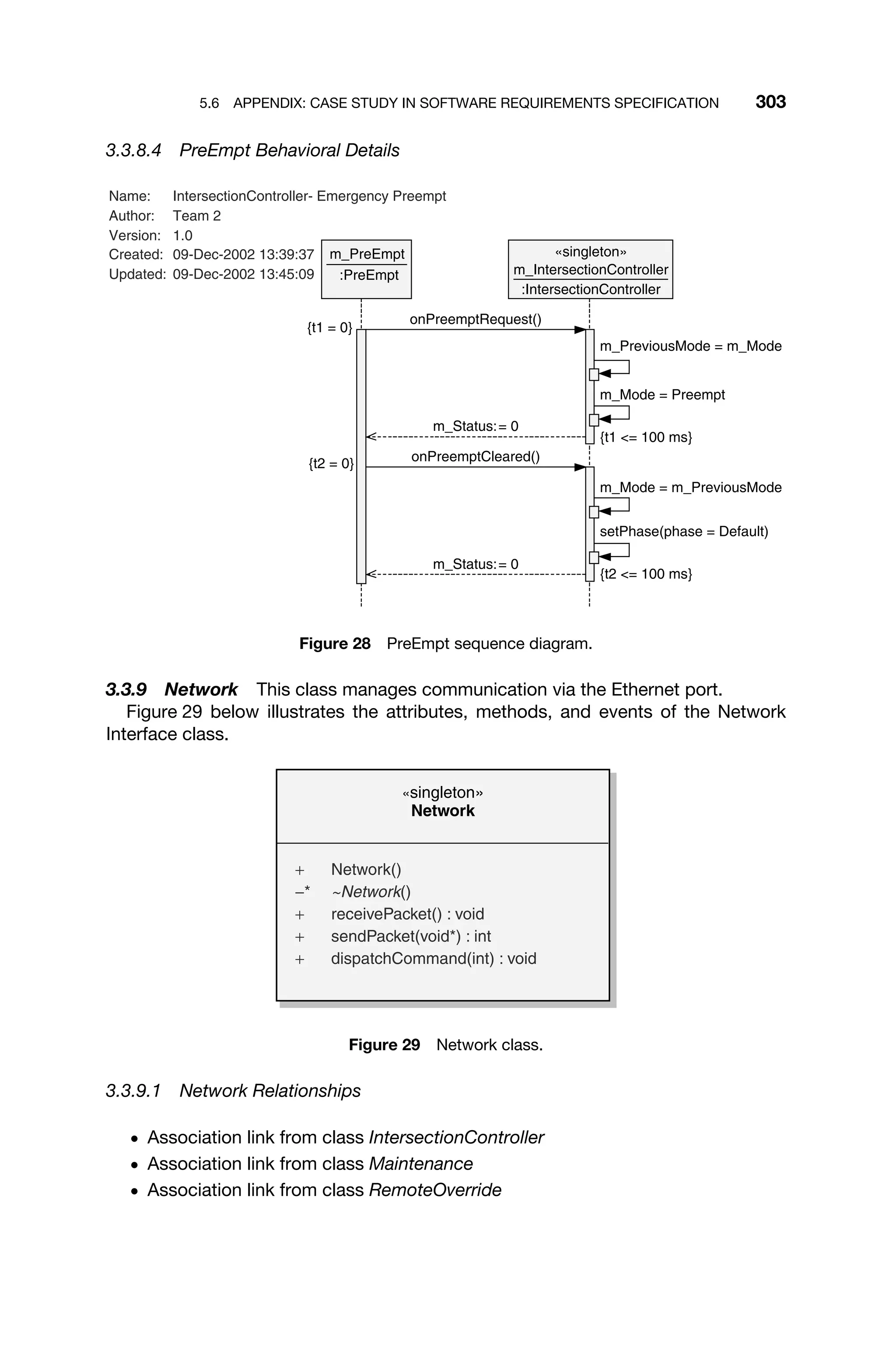
![304 5 SOFTWARE SYSTEM DESIGN
3.3.9.2 Network Methods
Table 25 Network class-methods
Method Type Notes
Network () public: Constructor.
∼ Network () private abstract: Destructor.
receivePacket () public: void Method responsible for receiving network SNMP
packets.
sendPacket (void∗
) public: int param: packet [void∗
- in]
Method responsible for sending network SNMP
packets.
dispatchCommand (int) public: void param: command [int - in]
Interprets the received SNMP packet and invokes
the appropriate method in response.
3.3.10 Maintenance This class provides a maintenance interface to the intersec-
tion controller, accessible either from the local maintenance Ethernet port or the
DOT WAN.
The Maintenance class is responsible for managing the following functions:
1. Retrieval of database information.
2. Retrieval of current intersection controller status.
«singleton»
Maintenance
− m_Network: Network*
− m_IntersectionController: IntersectionController*
+ Maintenance()
−* ~Maintenance()
+ readDatabase(int) : void
+ getStatus() : Phase
Figure 30 Maintenance class.
3.3.10.1 Maintenance Relationships
ž Association link to class IntersectionController
ž Association link to class Network](https://image.slidesharecdn.com/epdf-230618090952-bdcb6616/75/epdf-pub_real-time-systems-design-and-analysis-pdf-327-2048.jpg)
![5.6 APPENDIX: CASE STUDY IN SOFTWARE REQUIREMENTS SPECIFICATION 305
3.3.10.2 Maintenance Attributes
Table 26 Maintenance class-attributes
Attribute Type Notes
m Network private: Network Pointer to the m Network object.
m IntersectionController private:
IntersectionController
Pointer to the
m IntersectionController object.
3.3.10.3 Maintenance Methods
Table 27 Maintenance class-methods
Method Type Notes
Maintenance () public: Constructor.
∼ Maintenance () private abstract: Destructor.
readDatabase (int) public: void param: database [int - in]
Method to read the contents of the database specified
by the parameter database.
getStatus () public: Phase Method to get the intersection status.
3.3.11 Database (Traffic History; Incident Log) Instances of this class are used
to store the Traffic History and the Incident Log for the intersection being controlled.
The Traffic History object is responsible for managing the following functions:
1. Storage and retrieval of traffic history database records.
2. Clearing of traffic history in response to a command from a remote host.
Figure 31 illustrates the attributes, methods, and events of the Traffic History class.](https://image.slidesharecdn.com/epdf-230618090952-bdcb6616/75/epdf-pub_real-time-systems-design-and-analysis-pdf-328-2048.jpg)
![306 5 SOFTWARE SYSTEM DESIGN
Database
{2}
− MAXRECORDS: int
− m_Record: Record* [0..* ordered]
− m_CurrentRecord: int
− m_First: int
− m_Last: int
− m_Full: boolean
+ Database()
−* ~Database()
+ goFirst() : int
+ goLast() : int
+ goNext() : int
+ go(int) : int
+ isFull() : boolean
+ isEOF() : boolean
+ read() : Record
+ read(int) : Record
+ write(Record*) : int
+ write(int, Record*) : int
+ flush() : int
Figure 31 Database class.
3.3.11.1 Database Relationships
ž Association link to class Record
ž Association link from class IntersectionController
ž Association link from class IntersectionController
3.3.11.2 Database Attributes
Table 28 Database class-attributes
Attribute Type Notes
MAXRECORDS private: int Constant defining the maximum number of records
permitted.
m Record private: Record Pointer to database records, which are of type
Record.
m CurrentRecord private: int Position (index) of current record.
m First private: int Position (index) of first (least recent) record in FIFO
database structure.](https://image.slidesharecdn.com/epdf-230618090952-bdcb6616/75/epdf-pub_real-time-systems-design-and-analysis-pdf-329-2048.jpg)
![5.6 APPENDIX: CASE STUDY IN SOFTWARE REQUIREMENTS SPECIFICATION 307
Table 28 (continued)
Attribute Type Notes
m Last private: int Position (index) of last (most recent) record in FIFO
database structure.
m Full private: boolean True if data is being overwritten.
3.3.11.3 Database Methods
Table 29 Database class-methods
Method Type Notes
Database () public: Constructor.
∼ Database () private abstract: Destructor.
goFirst () public: int Move cursor to first (least recent) record. Completes
in 40 ms.
goLast () public: int Move cursor to last (most recent) record. Completes
in 40 ms.
goNext () public: int Move cursor to the next record. Completes in 40 ms.
go (int) public: int param: record [int - in]
Move cursor to the specified record. Completes in
40 ms.
isFull () public: boolean True if the database is full. Subsequent writes will
overwrite oldest data (FIFO).
isEOF () public: boolean True when the cursor is at the last record.
read () public: Record Read record at current position. Completes in 10 ms.
read (int) public: Record param: position [int - in]
Read record at specified position; update current
record to specified position. Completes in 50 ms.
write (Record∗
) public: int param: record [Record∗
- inout]
Add new record to end of database. If isFull() is
True, data will be overwritten. Completes in
50 ms.
write (int, Record∗
) public: int param: position [int - in]
param: record [Record∗
- inout]
(continued)](https://image.slidesharecdn.com/epdf-230618090952-bdcb6616/75/epdf-pub_real-time-systems-design-and-analysis-pdf-330-2048.jpg)
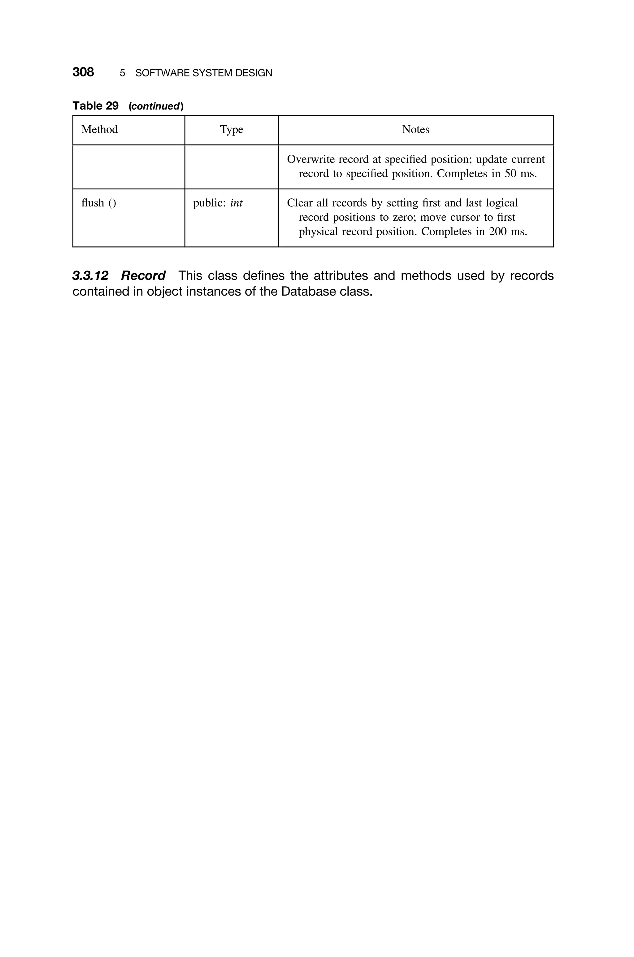
![5.6 APPENDIX: CASE STUDY IN SOFTWARE REQUIREMENTS SPECIFICATION 309
Database
{2}
− MAXRECORDS: int = 65536
− m_Record: Record* [0..* ordered]
− m_CurrentRecord: int
− m_First: int
− m_Last: int
− m_Full: boolean
+ Database()
−* ~Database()
+ goFirst() : int
+ goLast() : int
+ goNext() : int
+ go(int) : int
+ isFull() : boolean
+ isEOF() : boolean
+ read() : Record
+ read(int) : Record
+ write(Record*) : int
+ write(int, Record*) : int
+ flush() : int
Record
− timestamp: datetime
− source: int
− data: string
+ Record()
−* ~Record()
+ setTimestamp(datetime*) : void
+ setSource(int) : void
+ setData(string*) : void
+ getTimestamp() : datetime
+ getSource() : int
+ getData() : string
0..* {ordered}
+m_Record
Figure 32 Record class.](https://image.slidesharecdn.com/epdf-230618090952-bdcb6616/75/epdf-pub_real-time-systems-design-and-analysis-pdf-332-2048.jpg)
![310 5 SOFTWARE SYSTEM DESIGN
3.3.12.1 Record Relationships
ž Association link from class Database
3.3.12.2 Record Attributes
String of bytes containing the actual data.
private: string
data
Integer value representing the object that is the
source of the database record.
private: int
source
Date and time of the incident or traffic history
entry.
private: datetime
timestamp
Notes
Type
Attribute
Figure 33 Record class-attributes.
3.3.12.3 Record Methods
public: string
public: int
public: datetime
public: void
public: void
public: void
private abstract:
public:
Accessor for m_Data attribute.
Accessor for m_Source attribute.
Accessor for m_Timestamp attribute.
param: data [ string - inout]
Mutator for m_Data attribute.
param: source [ int - in ]
param: timestamp [ datetime - inout]
Mutator for m_Timestamp attribute.
Destructor.
Constructor.
getData()
getSource()
getTimestamp()
setData (string)
setSource (int)
setTimestamp (datetime)
~Record ()
Record ()
Notes
Type
Method
Figure 34 Record class-methods.
3.3.13 ErrorHandler This class handles all errors generated by the application.
All errors are generated by the IntersectionController class, in response either to
internal errors or error returns from method calls.
3.3.13.1 ErrorHandler Relationships
ž Association link from class IntersectionController](https://image.slidesharecdn.com/epdf-230618090952-bdcb6616/75/epdf-pub_real-time-systems-design-and-analysis-pdf-333-2048.jpg)
![5.6 APPENDIX: CASE STUDY IN SOFTWARE REQUIREMENTS SPECIFICATION 311
3.3.13.2 ErrorHandler Methods
param: error [ int - in ]
Attempts to set the intersection to the default
phase. If unsuccessful, attempts a reset. If this
fails or the error occurs again immediately after
reset, the watchdog timer will override software
error handling.
Logs the error and sends a network message to
the DOT central office via the DOT WAN.
public: void
onCriticalError (int)
param: error [ int - in ]
Logs the error incident and resumes normal
operation.
public: void
onNonCriticalError (int)
Destructor.
private abstract:
~ErrorHandler()
Constructor.
public:
ErrorHandler()
Notes
Type
Method
Figure 35 ErrorHandler class-methods.
3.3.13.3 ErrorHandler Behavioral Details
«singleton»
m_ErrorHandler
:ErrorHandler
«singleton»
m_IntersectionController
:IntersectionController
m_IncidentLog
:Database
Name: IntersectionController- Non-Critical Error Handling
Author: Team 2
Version: 1.0
Created: 09-Dec-2002 11:46:49
Updated: 09-Dec-2002 11:53:07
{t = 0}
onNonCriticalError(error)
{t = 500 ms} write(record)
Figure 36 Noncritical error sequence diagram.](https://image.slidesharecdn.com/epdf-230618090952-bdcb6616/75/epdf-pub_real-time-systems-design-and-analysis-pdf-334-2048.jpg)
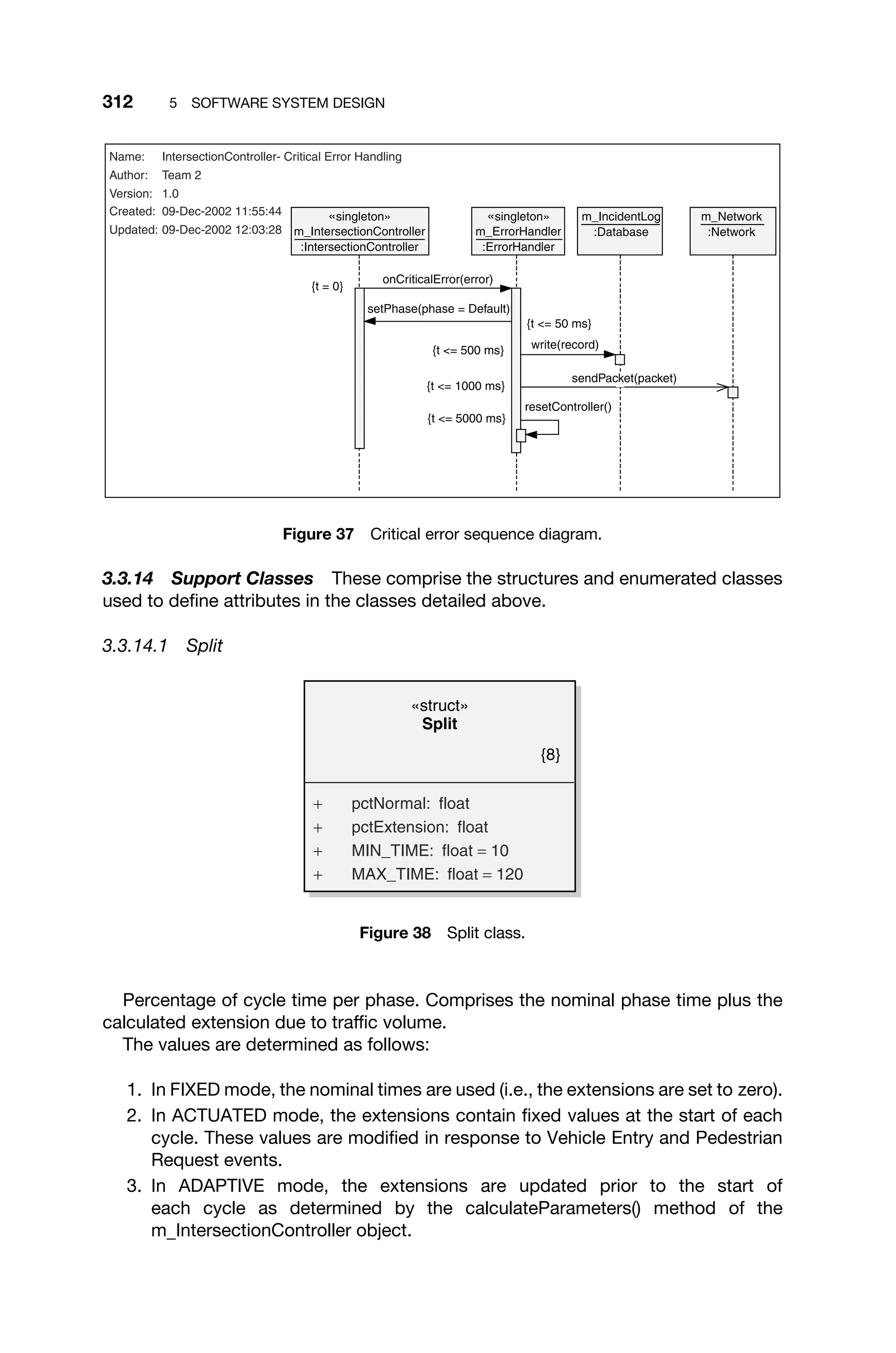
![5.6 APPENDIX: CASE STUDY IN SOFTWARE REQUIREMENTS SPECIFICATION 313
3.3.14.1.1 SPLIT RELATIONSHIPS
ž Association link from class Parameters
3.3.14.2 Parameters
«struct»
Parameters
+ cycleTime: float
+ splits: Split* [8 ordered]
Figure 39 Parameters class.
3.3.14.2.1 PARAMETERS RELATIONSHIPS
ž Association link from class Status
ž Association link to class Split
ž Association link from class IntersectionController
3.3.14.3 Status
«struct»
Status
+ mode: Mode
+ count: int* [4 ordered]
+ parameters: Parameters*
+ phase: Phase
Figure 40 Status class.
3.3.14.3.1 STATUS RELATIONSHIPS
ž Association link to class Parameters
ž Association link to class IntersectionController
ž Dependency link from class RemoteOverride
ž Association link to class Mode
ž Association link to class Phase](https://image.slidesharecdn.com/epdf-230618090952-bdcb6616/75/epdf-pub_real-time-systems-design-and-analysis-pdf-336-2048.jpg)
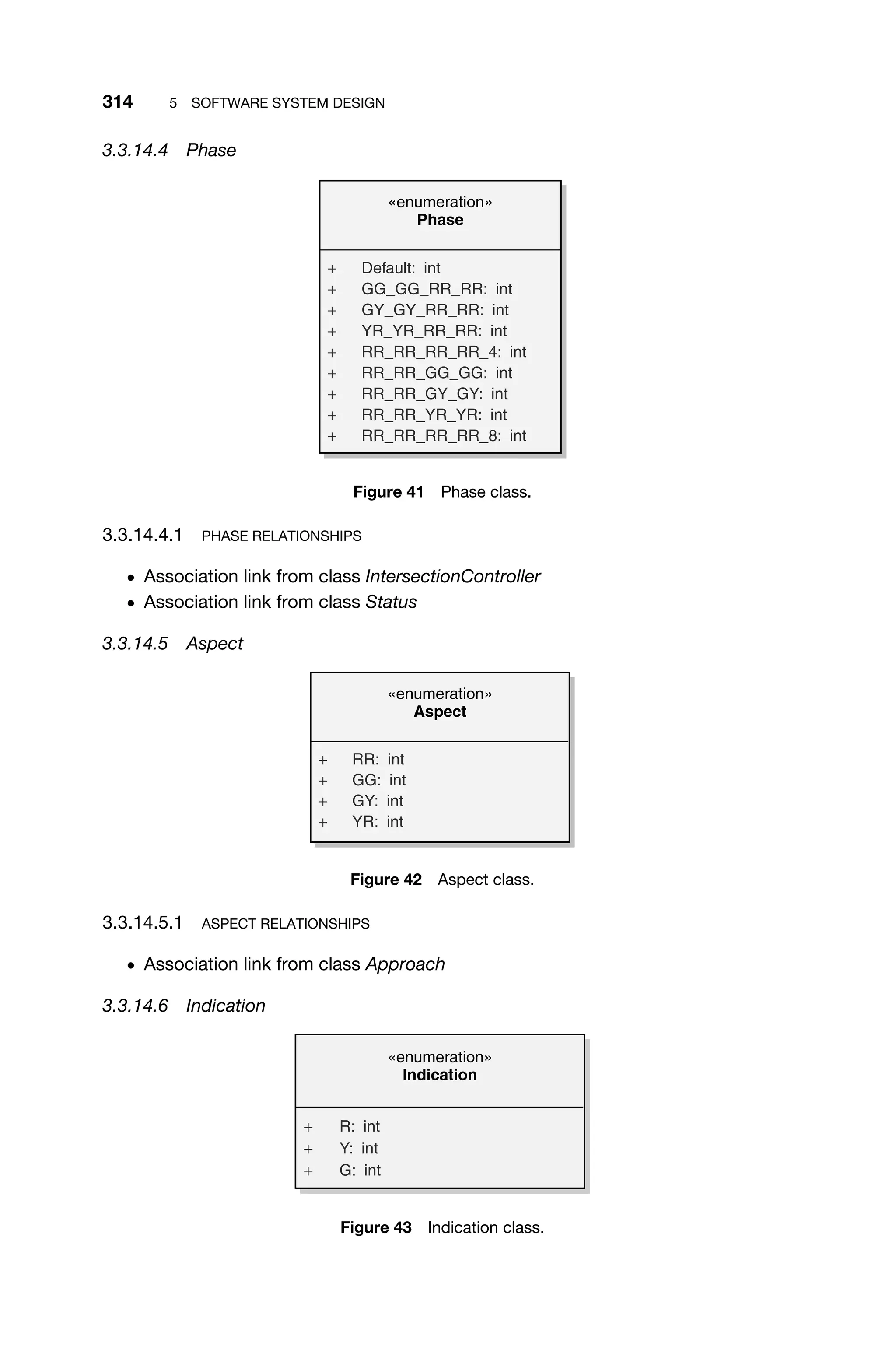
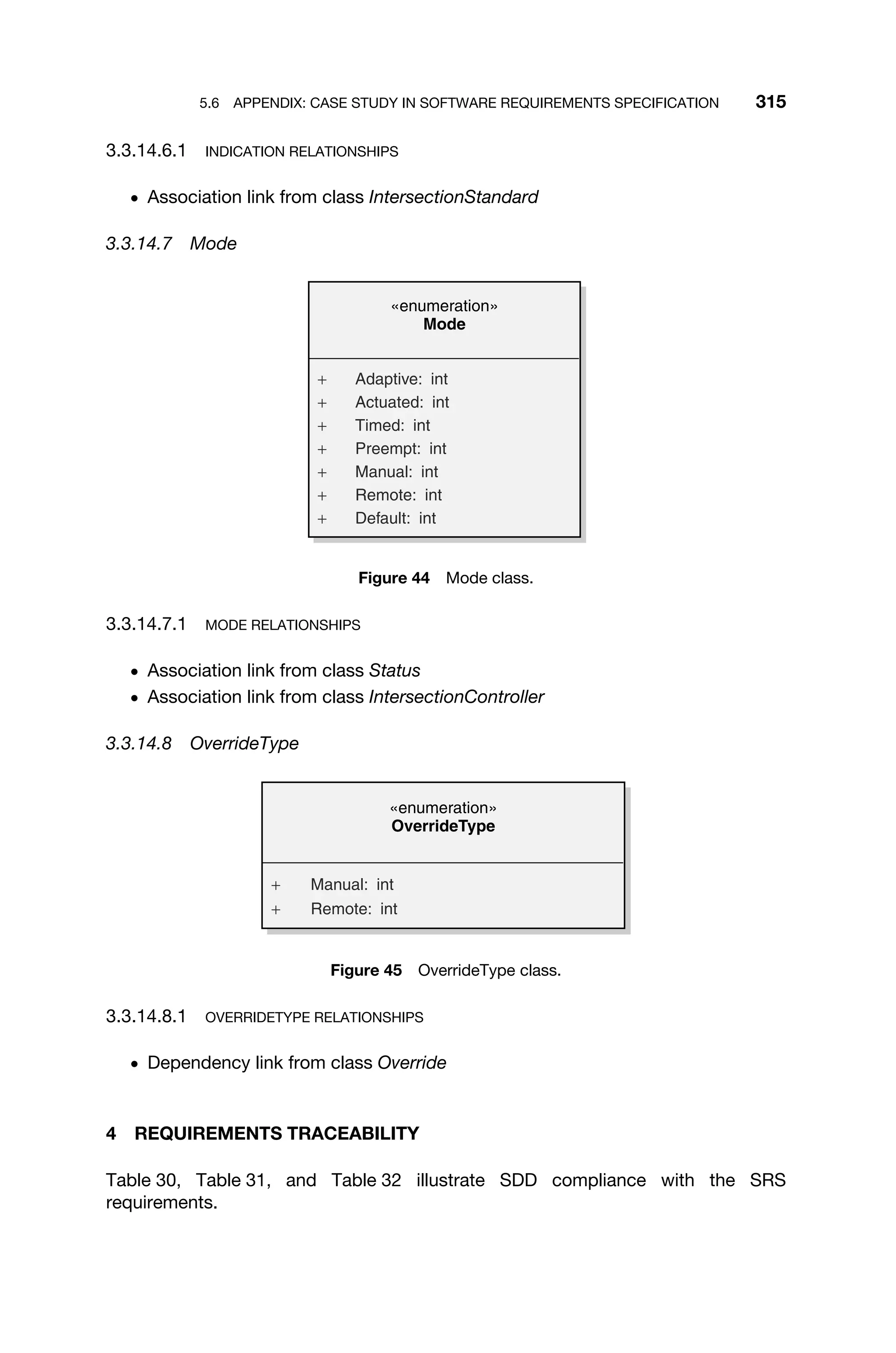
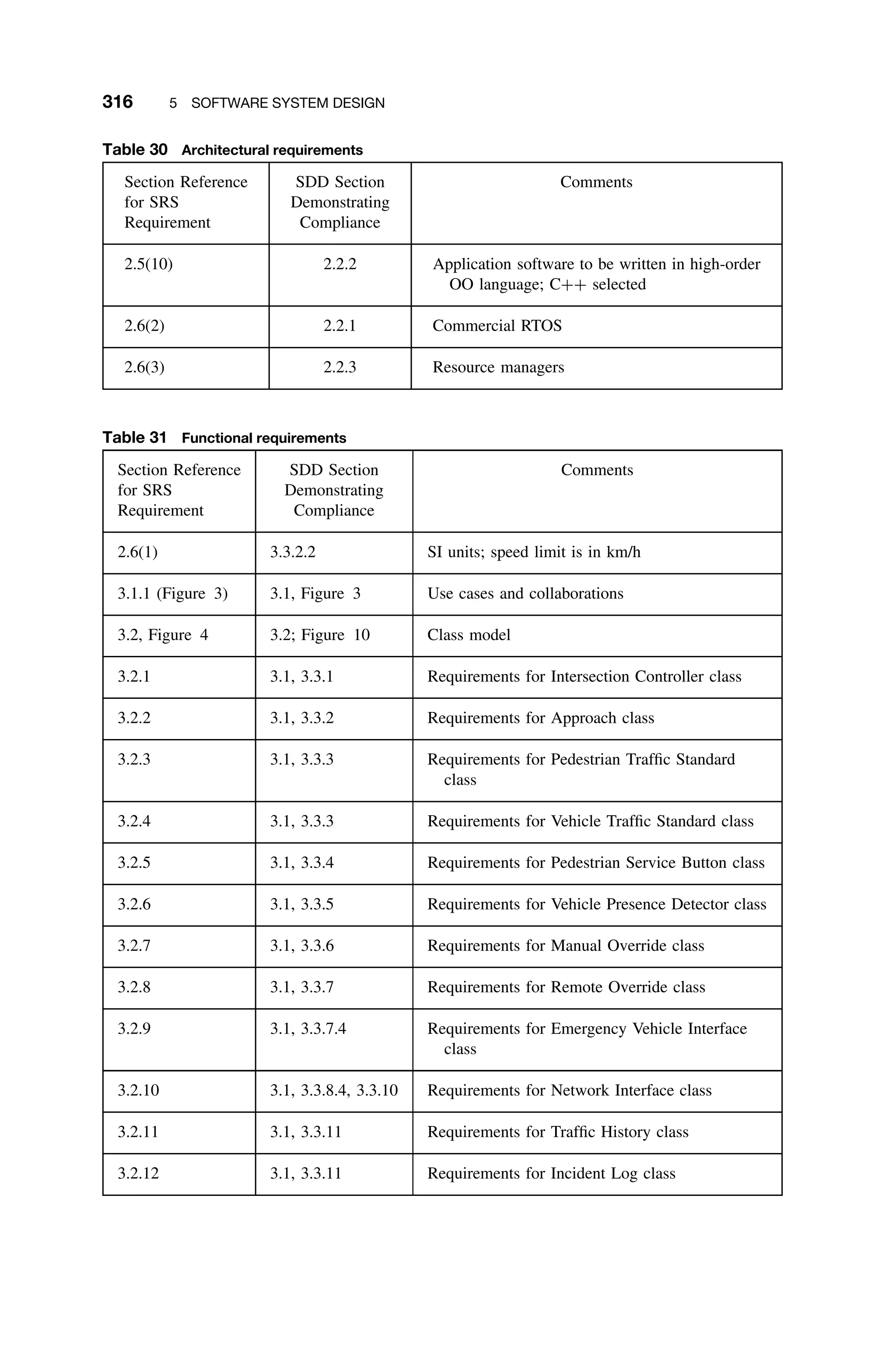
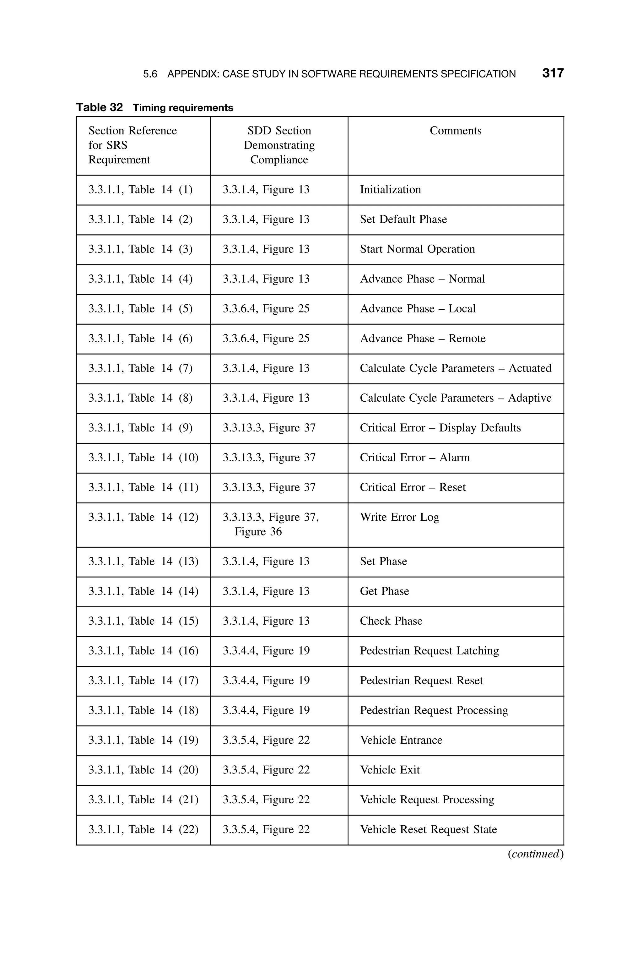
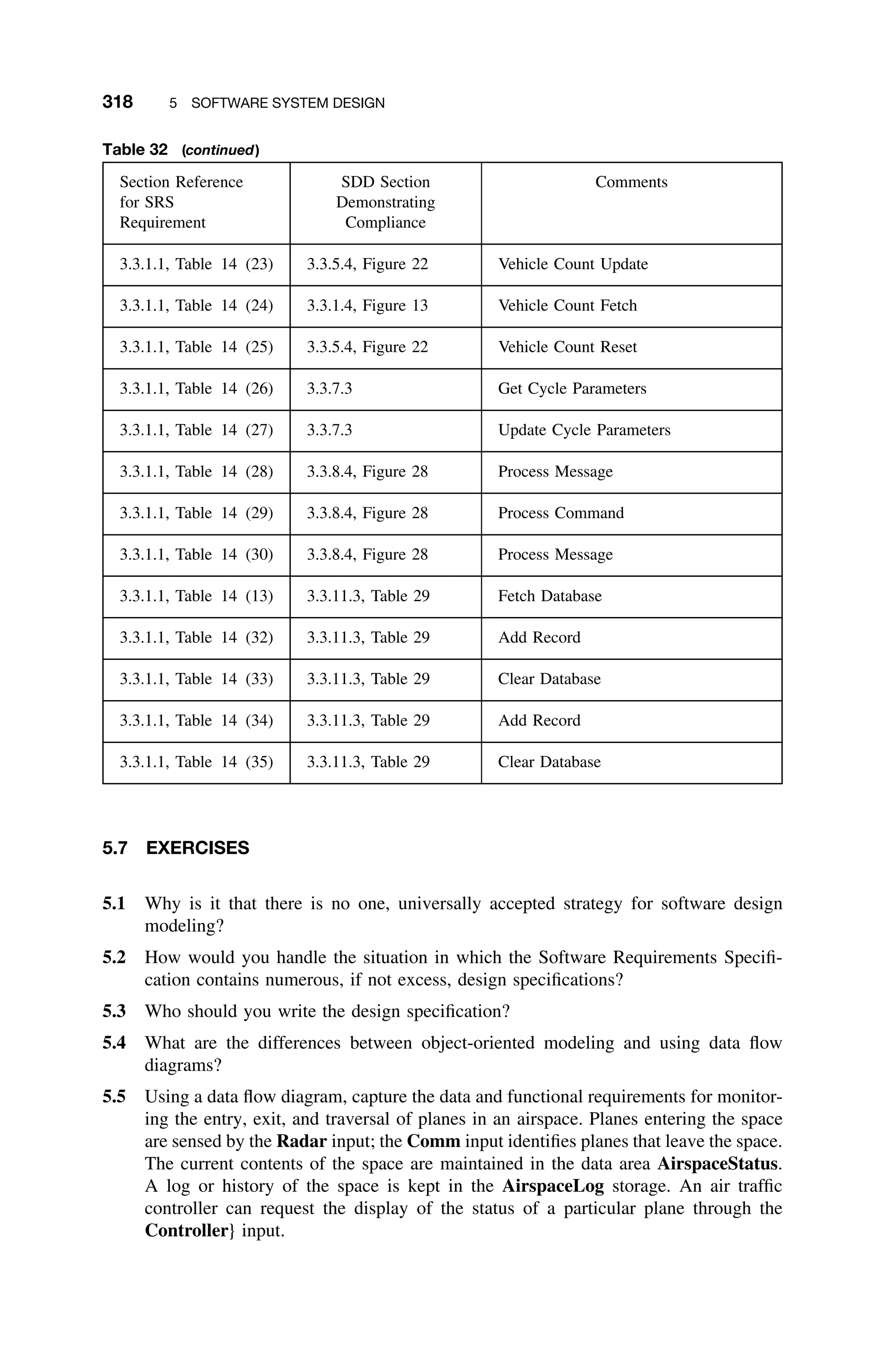

![322 6 PROGRAMMING LANGUAGES AND THE SOFTWARE PRODUCTION PROCESS
including various dialects of C, C++, C#, Java, Fortran, Pascal, Ada 95, assembly
language, and even Visual BASIC, and Basic.
Of this list C++, Java, and C# are object-oriented, while the others are pro-
cedural. Ada 95 has elements of both object-oriented and procedural languages,
and can be used either way, depending on the skill and preferences of the pro-
grammer. Applicative languages such as LISP and Prolog have also been used to
build real-time systems [Allard91], but this is rather unusual and this discussion
of languages is confined to those just listed.
An appropriate question is: “What is the fitness of a language for real-time
applications and what criteria can be used to measure such fitness?” To answer
this consider the following (informal) metrics [Cardelli96]:
ž Economy of Execution How fast does a program run?
ž Economy of Compilation How long does it take to go from sources to
executables?
ž Economy of Small-Scale Development How hard must an individual pro-
grammer work?
ž Economy of Large-Scale Development How hard must a team of program-
mers work?
ž Economy of Language Features How hard is it to learn or use a program-
ming language?
Each programming language offers its own strengths and weaknesses with
respect to real-time systems, and these criteria can be used to calibrate the
features of a particular language for apples-to-apples comparison for a given
application.
The focus of this chapter is on those language features that minimize the final
code execution time and that lend themselves to performance prediction.
The compile time prediction of execution time performance is known as a
schedulability analysis. In the design of modern real-time languages, the emphasis
is on eliminating those constructs that render the language nonanalyzable, for
example, unbounded recursion and unbounded while loops. Most so-called “real
time languages” strive to eliminate all of these.
6.2 ASSEMBLY LANGUAGE
Although lacking most of the features of high-level languages, assembly language
does have certain advantages for use in real-time systems, in that it provides more
direct control of the computer hardware. Unfortunately, assembly language is
unstructured and has limited abstraction properties. It varies widely from machine
to machine. Coding in assembly language is usually difficult to learn, tedious,
and error prone. Finally, the resulting code is nonportable. Therefore its use in
embedded real-time systems is discouraged.](https://image.slidesharecdn.com/epdf-230618090952-bdcb6616/75/epdf-pub_real-time-systems-design-and-analysis-pdf-345-2048.jpg)
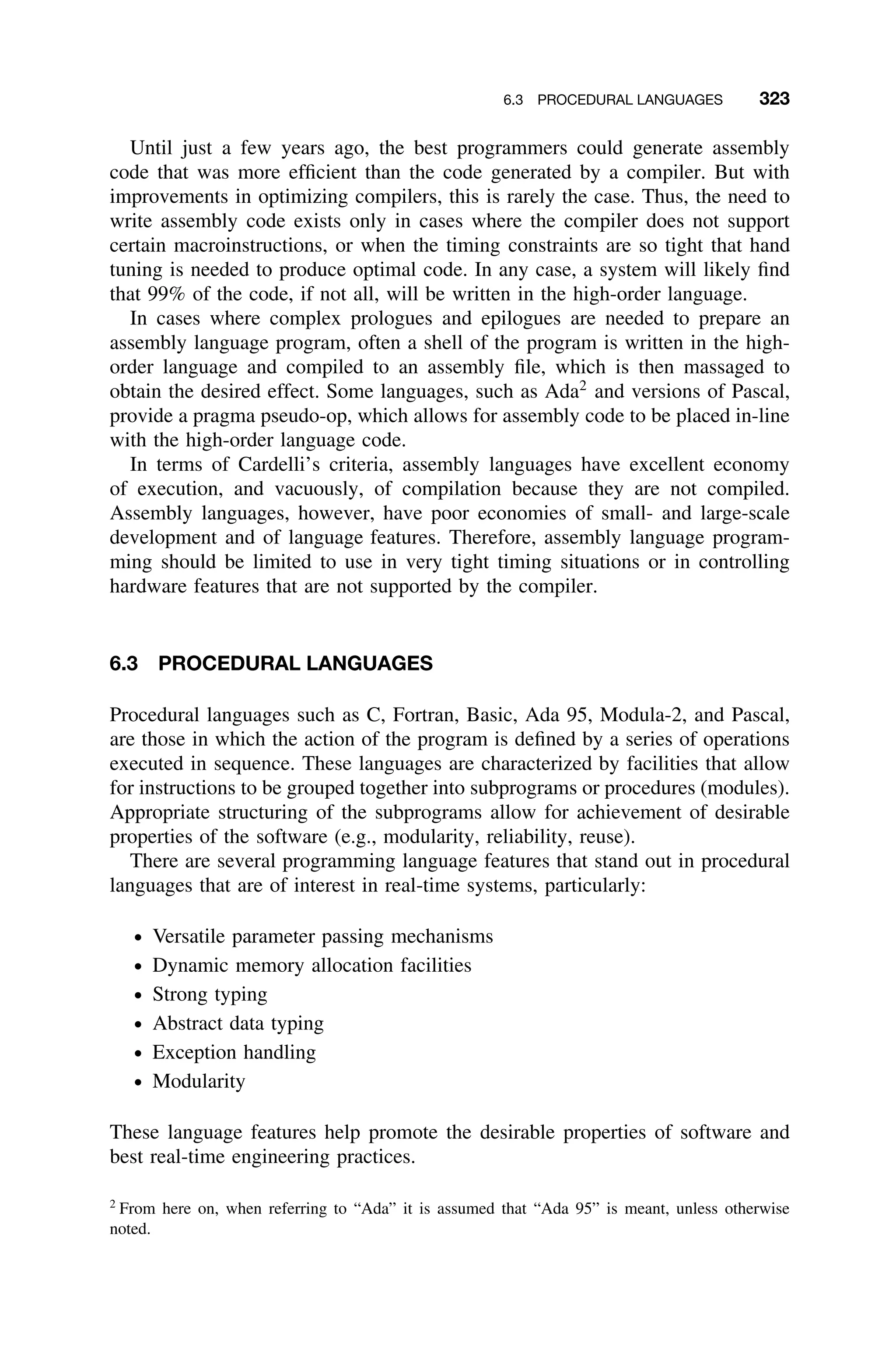
![6.4 OBJECT-ORIENTED LANGUAGES 329
While modular software is desirable, there is a price to pay in the overhead
associated with procedure calls and parameter passing. This adverse effect should
be considered when sizing modules.
6.3.9 Cardelli’s Metrics and Procedural Languages
Taking the set of procedural languages as a whole, Cardelli considered them
for use in real-time systems with respect to his criteria. His comments are
paraphrased in the foregoing discussion. First, he notes that variable typing
was introduced to improve code generation. This was particularly true in the
case of Fortran. Hence, economy of execution is high for procedural languages
provided the compiler is efficient. Further, because modules can be compiled
independently compilation of large systems is efficient, at least when inter-
faces are stable. The more challenging aspects of system integration are thus
eliminated.
Small-scale development is economical because type checking can catch many
coding errors, reducing testing and debugging efforts. The errors that do occur
are easier to debug, simply because large classes of other errors have been ruled
out. Finally, experienced programmers adopt a coding style that causes some
logical errors to show up as type checking errors hence they can use the type
checker as a development tool. For example, changing the name of a type when
its invariants change even though the type structure remains the same, yields
error reports on all its old uses.
In addition, data abstraction and modularization have methodological advan-
tages for large-scale code development. Large teams of programmers can nego-
tiate the interfaces to be implemented, and then proceed separately to implement
the corresponding pieces of code. Dependencies between pieces of code are
minimized, and code can be locally rearranged without fear of global effects.
Finally, procedural languages are economical because some well-designed con-
structions can be naturally composed in orthogonal ways. For example, in C an
array of arrays models two-dimensional arrays. Orthogonality of language fea-
tures reduces the complexity of programming languages. The learning curve for
programmers is thus reduced, and the relearning effort that is constantly necessary
in using complex languages is minimized [Cardelli96].
6.4 OBJECT-ORIENTED LANGUAGES
The benefits of object-oriented techniques are well known, for example, increas-
ing programmer efficiency, reliability, and the potential for reuse. Object-oriented
languages include Smalltalk, C++, Java, C#, Eiffel, and Ada 95 when so used.
Formally, object-oriented programming languages are those that support data
abstraction, inheritance, polymorphism, and messaging.
Objects are an effective way to manage system complexity, as they provide
a natural environment for information hiding, or protected variation and encap-
sulation. In encapsulation, a class of objects and methods associated with them](https://image.slidesharecdn.com/epdf-230618090952-bdcb6616/75/epdf-pub_real-time-systems-design-and-analysis-pdf-352-2048.jpg)
![6.4 OBJECT-ORIENTED LANGUAGES 331
Immutable Objects An immutable object’s state can never be modified after
it is instantiated. Therefore immutable objects require no synchronization
when accessed by multiple threads since all accesses are read-only.
Unsynchronized Objects Objects in a single-threaded program require no
synchronization.
To illustrate the necessity of supporting parameterization of synchronization
policies, consider a class library. A developer of a class library wants to ensure
the widest possible audience for this library, so he or she makes all classes
synchronized so that they can be used safely in both single-threaded and mul-
tithreaded applications. However, clients of the library whose applications are
single-threaded are unduly penalized with the unnecessary execution overhead of
synchronization that they do not need. Even multithreaded applications can be
unduly penalized if the objects do not require synchronization (e.g., the object
is thread-local). Therefore to promote reusability of a class library without sac-
rificing performance, classes in a library ideally would allow clients to select on
a per-object basis which synchronization policy to use.
6.4.2 4
Garbage Collection
Recall that garbage refers to allocated memory that is no longer being used but is
not otherwise available. Excessive garbage accumulation can be detrimental and
therefore garbage must be reclaimed. Garbage collection algorithms generally
have unpredictable performance (although average performance may be known).
Garbage can be created in both procedural and object-oriented languages. For
example, in Pascal or C, garbage can be created by allocating memory, but not
deallocating it properly. But garbage is generally associated with object-oriented
languages like C++ and Java. Java is noteworthy in that the standard envi-
ronment incorporates garbage collection, whereas C++ does not. Therefore this
discussion of garbage collection strategies centers on Java. It is an interesting case
study in comparing several possible solutions to a real-time problem, involving
dynamic memory management, recursion, and bounded performance.
Java garbage collection routines allocate objects in a memory area called the
Java virtual machine (JVM) garbage-collection heap. Unlike traditional heaps for
a process’ virtual memory space, the garbage collector threads monitor objects in
use. Once the garbage collection routines determine that an object is unreachable,
the garbage collector automatically returns that object’s memory to the system.
Because the JVM specification does not specify how to free the memory, a JVM
can implement one of several garbage collection strategies, including:
ž Mark and sweep
ž Generational collection
ž Reference counting
4
Much of this section is adapted from [Lo03] is adapted from [Lo03] with permission.](https://image.slidesharecdn.com/epdf-230618090952-bdcb6616/75/epdf-pub_real-time-systems-design-and-analysis-pdf-354-2048.jpg)
![6.4 OBJECT-ORIENTED LANGUAGES 333
threads from modifying the object reference graph. This is one way to synchronize
program execution with garbage collection. However, the suspension could result
in a long garbage collection pause with no progress in program execution.
Typically, the shorter the garbage collection pause, the better the performance
of garbage collection. Although stop-the-world garbage collection involves a
garbage collection pause, it does not need a sophisticated synchronization mecha-
nism. The mechanism that suspends the program threads when garbage collection
threads are running tends to result in a smaller memory footprint. Stop-the-world
garbage collection is not the only garbage collector to induce a garbage collec-
tion pause. For example, the copying collector must stop the program threads
during copying, and the mark-compact algorithm requires suspending program
threads in its marking and copying phases. Whether the stop-the-world approach
is suitable for real-time systems depends on application requirements [Lo03].
Garbage collection algorithms generally have unpredictable performance (al-
though average performance may be known). The loss of determinism results
from the unknown amount of garbage, the tagging time of the nondeterministic
data structures, and the fact that many incremental garbage collectors require that
every memory allocation or deallocation from the heap be willing to service a
page-fault trap handler.
6.4.3 Cardelli’s Metrics and Object-Oriented Languages
Consider object-oriented languages in the context of Cardelli’s metrics as para-
phrased from his analysis. In terms of economy of execution, object-oriented
style is intrinsically less efficient than procedural style. In pure object-oriented
style, every routine is supposed to be a method. This introduces additional indi-
rections through method tables and prevents optimizations such as inlining. The
traditional solution to this problem (analyzing and compiling whole programs)
violates modularity and is not applicable to libraries.
With respect to economy of compilation, often there is no distinction between
the code and the interface of a class. Some object-oriented languages are not
sufficiently modular and require recompilation of superclasses when compiling
subclasses. Therefore, the time spent in compilation may grow disproportionately
with the size of the system.
On the other hand, object-oriented languages are superior with respect to econ-
omy of small-scale development. For example, individual programmers can take
advantage of class libraries and frameworks, drastically reducing their work
load. When the project scope grows, however, programmers must be able to
understand the details of those class libraries, and this turns out to be more
difficult than understanding module libraries. The type systems of most object-
oriented languages are not expressive enough; programmers must often resort
to dynamic checking or to unsafe features, damaging the robustness of their
programs.
In terms of economy of large-scale development, many developers are often
involved in developing class libraries and specializing existing class libraries.](https://image.slidesharecdn.com/epdf-230618090952-bdcb6616/75/epdf-pub_real-time-systems-design-and-analysis-pdf-356-2048.jpg)
![334 6 PROGRAMMING LANGUAGES AND THE SOFTWARE PRODUCTION PROCESS
Although reuse is a benefit of object-oriented languages, it is also the case that
these languages have extremely poor modularity properties with respect to class
extension and modification via inheritance. For example, it is easy to override a
method that should not be overridden, or to reimplement a class in a way that
causes problems in subclasses. Other large-scale development problems include
the confusion between classes and object types, which limits the construction
of abstractions, and the fact that subtype polymorphism is not good enough for
expressing container classes.
Object-oriented languages have low economy of language features. Smalltalk
was originally intended as a language that would be easy to learn. C++ is based
on a fairly simple model, inherited from Simula, but is overwhelming in the
complexity of its many features. Unfortunately, what started as economical and
uniform language (“everything is an object”) ended up as a vast collection of
class varieties. Java represents a step forward in the complexity trend, but is
more complex than most people realize [Cardelli96].
6.4.4 Object-Oriented versus Procedural Languages
There is still no agreement on which is better for real-time systems – object-
oriented or procedural languages. Even this author is somewhat conflicted. The
benefit of an object-oriented approach to problem solving and the use of object-
oriented languages are clear, and have already been described. Moreover, it is
possible to imagine certain aspects of an operating system that would benefit
from objectification, such as task, thread, file, or device, and certain applica-
tion domains can clearly benefit from an object-oriented approach. The main
arguments against object-oriented programming languages for real-time systems,
however, are that they can lead to unpredictable and inefficient systems and that
they are hard to optimize.
The unpredictability argument is hard to defend, however, at least with respect
to object-oriented languages, such as C++, that do not use garbage collection.
It is probably the case that a predictable system can be just as easily built in
C++ as C. Similarly, it is probably just as easy to build an unpredictable system
in C as in C++. The case for more unpredictable systems using object-oriented
languages is probably easier to sustain when arguing about garbage collecting
languages like Java.
In any case, the inefficiency argument against object-oriented languages is a
powerful one. Generally, there is an execution time penalty in object-oriented
languages in comparison to procedural languages. This “penalty” is due, in part,
to late binding (resolution of memory locations at run-time rather than at compile
time) necessitated by function polymorphism and inheritance. These represent
considerable and often nondeterministic delay factors. Another problem results
from the overhead of the garbage collection routines. One possible way to reduce
these penalties is not to define too many classes and only define classes that
contain coarse detail and high-level functionality.
Some anecdotal evidence illustrates that the use of object-oriented language for
real-time systems presents other, more subtle, difficulties. Consider the following](https://image.slidesharecdn.com/epdf-230618090952-bdcb6616/75/epdf-pub_real-time-systems-design-and-analysis-pdf-357-2048.jpg)
![6.4 OBJECT-ORIENTED LANGUAGES 335
vignette. A design team for a particular real-time system used Unified Modeling
Language (UML) diagrams and insisted that C++ be used to implement a fairly
simple and straightforward requirements specification. After coding was com-
plete, testing began. Although the system never failed, several users expressed the
desire to add a few requirements that would cause the system to miss deadlines.
A competing company that designed using a structured language met the new
requirements by optimizing the macroinstructions. They could do this because of
the close correspondence between the procedural code they had been written in
C and the actual instructions. This option was not available to developers using
C++.5
Such cases are frequently cited to dispute the viability of object-oriented
languages for real-time applications.
A more serious problem, perhaps, is the inheritance anomaly in object-oriented
languages. The inheritance anomaly arises when an attempt is made to use inher-
itance as a code reuse mechanism, which does not preserve substitutability (i.e.,
the subclass is not a subtype). If the substitutability were preserved, then the
anomaly would not occur. Since the use of inheritance for reuse has fallen out
of favor in object-oriented approaches (in favor of composition), however, it
seems that most inheritance anomaly rejections of object-oriented languages for
real-time focus reflects an antiquated view of object orientation.
Consider the following example from an excellent text on real-time operating
systems [Shaw01]:
BoundedBuffer
{
DEPOSIT
pre: not full
REMOVE
pre: not empty
}
MyBoundedBuffer extends BoundedBuffer
{
DEPOSIT
pre: not full
REMOVE
pre: not empty AND lastInvocationIsDeposit
}
Assuming that preconditions are checked and have “wait semantics” (i.e.,
wait for the precondition to become true), then clearly MyBoundedBuffer has
strengthened the precondition of BoundedBuffer, and hence violated substi-
tutability (and as such is a questionable use of inheritance).
Most opponents of object-oriented languages for real-time assert that concur-
rency and synchronization are poorly supported. However, when built-in language
support for concurrency does not exist, it is standard practice to create “wrapper
facade” classes to encapsulate system concurrency application program interface
(APIs) for use in object-orientation (e.g., wrapper classes in C++ for POSIX
5
Reported by one of the author’s clients who prefers to remain anonymous.](https://image.slidesharecdn.com/epdf-230618090952-bdcb6616/75/epdf-pub_real-time-systems-design-and-analysis-pdf-358-2048.jpg)
![336 6 PROGRAMMING LANGUAGES AND THE SOFTWARE PRODUCTION PROCESS
threads). Further, it has already been noted that there are several concurrency pat-
terns available for object-oriented real-time systems [Douglass03], [Schmidt00].
While concurrency may be poorly supported at the language level in practice, it
is not an issue since developers use libraries instead.
In summary, critics of object-oriented languages for real-time systems (includ-
ing, formerly, the author) seem fixated on Smalltalk and Java, ignoring C++.
C++ is probably more suitable for real-time since among other things it does not
have built-in garbage collection and class methods, and by default does not use
“dynamic binding.” In any case, there are no clear guidelines for where object-
oriented approaches and languages should be used. Each situation needs to be
considered separately.
6.5 BRIEF SURVEY OF LANGUAGES
For purposes of illustrating some of the aforementioned language properties it
is helpful to review some of the more widely used languages in real-time sys-
tems. The languages are presented in alphabetical order, and not in any rank of
endorsement.
Functional languages, such as LISP and ML, have been omitted from the
discussion. This is not because they are useless in the context of real-time appli-
cations, but simply because their use in this setting is rare. The discussion also
omits object-oriented scripting languages, which have become popular for writ-
ing tools, and test harnesses such as Python, Ruby, because they are generally
not appropriate for embedded targets.
6.5.1 Ada 95
Ada was originally intended to be the mandatory language for all U.S. Department
of Defense projects, which included a high percentage of embedded real-time
systems. The first version, which became standardized in 1983, had significant
problems. The programming language community had long been aware of the
problems with the first release of the Ada standard, and practically since the
first delivery of an Ada 83 compiler, had sought to resolve them, which resulted
in a new version. The new language, now called “Ada 95,” was the first inter-
nationally standardized object-oriented programming language. However, Ada’s
original intent has been consistently undermined by numerous exceptions that
were granted, and it seems inevitable that Ada is not destined to fulfill its origi-
nal intent.
Ada was intended to be designed specifically for embedded real-time systems,
but systems builders have typically found the language to be too bulky and
inefficient. Moreover, significant problems were found when trying to implement
multitasking using the limited tools supplied by the language, such as the roundly
criticized rendezvous mechanism.
Three pragmas were introduced in Ada 95 to resolve some of the uncertainty
in scheduling, resource contention, and synchronization.](https://image.slidesharecdn.com/epdf-230618090952-bdcb6616/75/epdf-pub_real-time-systems-design-and-analysis-pdf-359-2048.jpg)
![6.5 BRIEF SURVEY OF LANGUAGES 339
C code is organized into functions, which are global subroutines accessible to
a program. C++ added classes and class methods, which are functions that are
connected to classes. C++ class methods are very similar to Java class methods.
However, because C++ still supports C, there is nothing to discourage C++
programmers from using functions. This results in a mixture of function and
method use that makes for confusing programs.
Multiple inheritance is a feature of C++ that allows a class to be derived from
multiple parent classes. Although multiple inheritance is indeed powerful, it is
difficult to use correctly and causes many problems otherwise. It is also very
complicated to implement from the compiler perspective. The unwanted goto
statement has all but disappeared in C++, although technically it is still a part
of the language.
Significantly, more embedded systems are being constructed in C++ and many
practitioners are asking, “Should I implement the system in C or C++?” The
answer is always “it depends.” Choosing C in lieu of C++ in real-time embed-
ded applications is, roughly speaking, a trade-off between a “lean and mean”
C program that will be faster and easier to predict but harder to maintain, and
a C++ program that will be slower and unpredictable but potentially easier
to maintain.
C++ still allows for low-level control, for example, it can use inline methods
rather than a runtime call. This kind of implementation is not completely abstract,
nor completely low-level, but is acceptable in embedded environments.
To its detriment, there is some tendency to take existing C code and objectify
it by wrapping the procedural code into objects with little regard for the best
practices of object-orientation. This kind of approach is to be avoided because
it has the potential to incorporate all of the disadvantages of C++ and none
of the benefits. C++ also does not provide automatic garbage collection, which
means dynamic memory must be managed manually or garbage collection must
be home grown.
6.5.4 C#
C#6
is a C++-like language that, along with its operating environment, has simi-
larities to the JVM and Java, respectively. C# is associated with Microsoft’s. NET
Framework for scaled-down operating systems like Windows CE 3.0. Windows
CE 3.0 is highly configurable, capable of scaling from small, embedded sys-
tem footprints (350 KB) and upwards (e.g., for systems requiring user interface
support). The minimum kernel configuration provides basic networking support,
thread management, dynamic link library support, and virtual memory manage-
ment. While a detailed discussion is outside the scope of this text, it is clear
that Windows CE 3.0 was intended as a real-time operating system for the. NET
Platform.
C# supports “unsafe code,” allowing pointers to refer to specific memory loca-
tions. Objects referenced by pointers must be “pinned,” disallowing the garbage
6
Much of this discussion is adapted from [Lutz03].](https://image.slidesharecdn.com/epdf-230618090952-bdcb6616/75/epdf-pub_real-time-systems-design-and-analysis-pdf-362-2048.jpg)
![340 6 PROGRAMMING LANGUAGES AND THE SOFTWARE PRODUCTION PROCESS
collector from altering their location in memory. The garbage collector collects
pinned objects, it just does not move them. This capability would tend to increase
schedulability, and it also allows for DMA device access to write to specific
memory locations, a necessary capability in embedded real-time systems. .NET
currently offers a generational approach to garbage collection intended to min-
imize thread blockage during mark and sweep. For instance, a means to create
a thread at a particular instant, and guarantee the thread completes by a partic-
ular point in time, is not supported. C# supports many thread synchronization
mechanisms, but none with this level of precision. C# supports an array of thread
synchronization constructs: (1) lock, (2) monitor, (3) mutex, and (4) interlock. A
Lock is semantically identical to a critical section – a code segment guarantee-
ing entry into itself by only one thread at a time. Lock is shorthand notation for
the monitor class type. A mutex is semantically equivalent to a lock, with the
additional capability of working across process spaces. The downside to mutexes
is their performance cost. Finally, interlock, a set of overloaded static methods,
is used to increment and decrement numerics in a thread safe manner in order to
implement the priority inheritance protocol.
Timers that are similar in functionality to the existing Win32 timer exist in
C#. When constructed, timers are told how long to wait in milliseconds before
their first invocation, and are also supplied an interval, again in milliseconds,
specifying the period between subsequent invocations. The accuracy of these
timers is machine dependent, and not guaranteed, reducing their usefulness for
real-time systems.
C# and the. NET platform may not be appropriate for hard real-time systems
for several reasons, including the unbounded execution of its garbage collected
environment and its lack of threading constructs to adequately support schedu-
lability and determinism. It is possible that C# and. NET might be appropriate
for some soft and firm real-time systems, provided that these shortcomings are
not critical.
Indeed, C#’s ability to interact with operating system API’s, shield develop-
ers from complex memory-management logic, and floating-point performance
approaching C make it a platform that is possibly appropriate for certain soft and
even firm applications. However, disciplined programming would be required
[Lutz03].
6.5.5 Fortran
The Fortran7
language is the oldest high-order language used in modern real-time
systems (developed circa 1955). Because in its earlier versions it lacked recursion
and dynamic allocation facilities, embedded systems written in this language
typically included a large portion of assembly language code to handle interrupts
and scheduling, and communication with external devices was through the use
of memory-mapped I/O, direct memory access (DMA), and I/O instructions.
7
Although Fortran is an acronym for Formula Translator, it is often written as “Fortran” because
the word has entered the mainstream in the same way that the acronyms “laser” and “sonar” have.](https://image.slidesharecdn.com/epdf-230618090952-bdcb6616/75/epdf-pub_real-time-systems-design-and-analysis-pdf-363-2048.jpg)
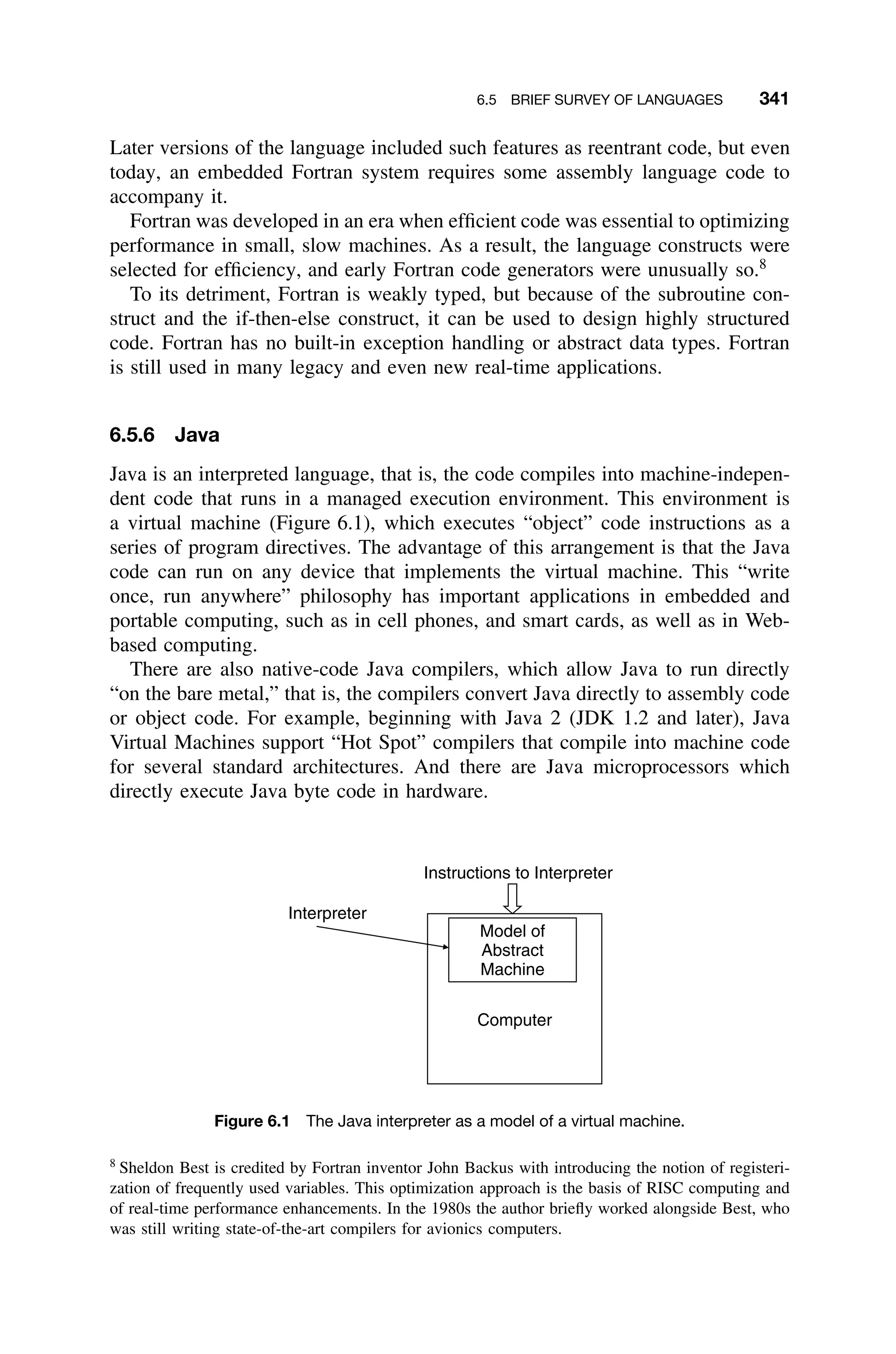
![344 6 PROGRAMMING LANGUAGES AND THE SOFTWARE PRODUCTION PROCESS
The RTSJ satisfies all but the first requirement, which was considered irrelevant
because access to physical memory is not part of the NIST requirements, but
industry input led the group to include it [Bollella00a].
6.5.6.2 Implementation of Real-Time Java The RTSJ defines the real-
time thread (RT) class to create threads, which the resident scheduler executes.9
RT threads can access objects on the heap, and therefore can incur delays because
of garbage collection.
For garbage collection, the RTSJ extends the memory model to support memory
management in a way that does not interfere with the real-time code’s abil-
ity to provide deterministic behavior. These extensions allow both short- and
long-lived objects to be allocated outside the garbage-collection heap. There is
also sufficient flexibility to use familiar solutions, such as preallocated object
pools.
RTSJ uses “priority” somewhat more loosely than is traditionally accepted.
“Highest priority thread” merely indicates the most eligible thread – the thread
that the scheduler would choose from among all the threads ready to run. It does
not necessarily presume a strict priority-based dispatch mechanism.
The system must queue all threads waiting to acquire a resource in priority
order. These resources include the processor as well as synchronized blocks. If
the active scheduling policy permits threads with the same priority, the threads
are queued FIFO. Specifically, the system (1) orders waiting threads to enter
synchronized blocks in a priority queue; (2) adds a blocked thread that becomes
ready to run to the end of the run-ready queue for that priority; (3) adds a thread
whose priority is explicitly set by itself or another thread to the end of the run
ready queue for the new priority; and (4) places a thread that performs a yield
to the end of its priority queue. The Priority Inheritance Protocol is implemented
by default. The specification also provides a mechanism by which systemwide
default policy can be implemented.
The asynchronous event facility comprises two classes: AsyncEvent and
AsyncEventHandler. An AsyncEvent object represents something that can
happen – like a Posix signal or hardware interrupt – or it represents a computed
event – like an airplane entering a specified region. When one of these events
occurs, indicated by the fire() method being called, the system schedules
associated AsyncEventHandlers. An AsyncEvent manages two things: the
dispatching of handlers when the event is fired, and the set of handlers associated
with the event. The application can query this set and add or remove handlers. An
AsyncEventHandler is a schedulable object roughly similar to a thread. When
the event fires, the system invokes run() methods of the associated handlers.
9
Most of this discussion has been adapted from [Bollela00a].](https://image.slidesharecdn.com/epdf-230618090952-bdcb6616/75/epdf-pub_real-time-systems-design-and-analysis-pdf-367-2048.jpg)

![352 7 PERFORMANCE ANALYSIS AND OPTIMIZATION
transformable to it. A problem is NP-hard if all problems in NP are polynomial
transformable to that problem, but it hasn’t been shown that the problem is in
the class NP.
The Boolean Satisfiability Problem, for example, which arose during require-
ments consistency checking in Chapter 4 is NP-complete. NP-complete problems
tend to be those relating to resource allocation, which is exactly the situation that
occurs in real-time scheduling. This fact does not bode well for the solution of
real-time scheduling problems.
7.1.2 Challenges in Analyzing Real-Time Systems
The challenges in finding workable solutions for real-time scheduling problems
can be seen in more than 30 years of real-time systems research. Unfortunately
most important problems in real-time scheduling require either excessive practical
constraints to be solved or are NP-complete or NP-hard. Here is a sampling from
the literature as summarized in [Stankovic95].
1. When there are mutual exclusion constraints, it is impossible to find a
totally on-line optimal run-time scheduler.
2. The problem of deciding whether it is possible to schedule a set of periodic
processes that use semaphores only to enforce mutual exclusion is NP-hard.
3. The multiprocessor scheduling problem with two processors, no resources,
arbitrary partial-order relations, and every task having unit computation
time is polynomial. A partial-order relation indicates that any process can
call itself (reflexivity), if process A calls process B, then the reverse is not
possible (antisymmetry), and if process A calls process B and process B
calls process C, than process A can call process C (transitivity).
4. The multiprocessor scheduling problem with two processors, no resources,
independent tasks, and arbitrary computation times is NP-complete.
5. The multiprocessor scheduling problem with two processors, no resources,
independent tasks, arbitrary partial order, and task computation times of
either 1 or 2 units of time is NP-complete.
6. The multiprocessor scheduling problem with two processors, one resource,
a forest partial order (partial order on each processor), and each computation
time of every task equal to 1 is NP-complete.
7. The multiprocessor scheduling problem with three or more processors, one
resource, all independent tasks, and each computation time of every task
equal to 1 is NP-complete.
8. Earliest deadline scheduling is not optimal in the multiprocessing case.
9. For two or more processors, no deadline scheduling algorithm can be opti-
mal without complete a priori knowledge of deadlines, computation times,
and task start times,
It turns out that most multiprocessor scheduling problem are in NP, but for deter-
ministic scheduling this is not a major problem because a polynomial scheduling](https://image.slidesharecdn.com/epdf-230618090952-bdcb6616/75/epdf-pub_real-time-systems-design-and-analysis-pdf-375-2048.jpg)
![7.1 THEORETICAL PRELIMINARIES 353
algorithm can be used to develop an optimal schedule if the specific problem is
not NP-complete [Stankovic95]. In these cases, alternative, off-line heuristic search
techniques can be used. These off-line techniques usually only need to find feasible
schedules, not optimal ones. But this is what engineers do when workable theories
do not exist – engineering judgment must prevail.
7.1.3 The Halting Problem
The Halting Problem, simply stated, is: does there exist a computer program that
takes an arbitrary program, Pi, and an arbitrary set of inputs, Ij , and determines
whether or not Pi will halt on Ij (Figure 7.1). The question of the existence of
such an oracle is more than a theoretical exercise, and it has important impli-
cations in the development of process monitors, program verification, and in
schedulability analysis. Unfortunately, such an oracle cannot be built.1
Thus the
Halting Problem is unsolvable. There are several ways to demonstrate this sur-
prising fact. One way is using Cantor’s diagonal argument, first used to show
that the real numbers are not countably denumerable.
It should be clear that every possible program, in any computer language, can
be encoded using a numbering scheme in which each program is represented as
the binary expansion of the concatenated source-code bytes. The same encoding
can be used with each input set. Then if the proposed oracle could be built, its
behavior would be described in tabular form as in Table 7.1. That is, for each
program Pi and each input set Ij it would simply have to determine if program Pi
halts on Ij . Such an oracle would have to account for every conceivable program
and input set.
In Table 7.1, the ↑ symbol indicates that the program does not halt and the
symbol ↓ indicates that the program will halt on the corresponding input. How-
ever, the table is always incomplete in that a new program P ∗
can be found
Oracle
Set of Inputs to Program
Ij
Halt or No Halt
Decision
Arbitirary
Program pi
Source
Code
Figure 7.1 A graphical depiction of the Halting Problem.
1
Strictly speaking, such an oracle can be built if it is restricted to a computer with fixed-size
memory since, eventually, a maximum finite set of inputs would be reached, and hence the table
could be completed.](https://image.slidesharecdn.com/epdf-230618090952-bdcb6616/75/epdf-pub_real-time-systems-design-and-analysis-pdf-376-2048.jpg)
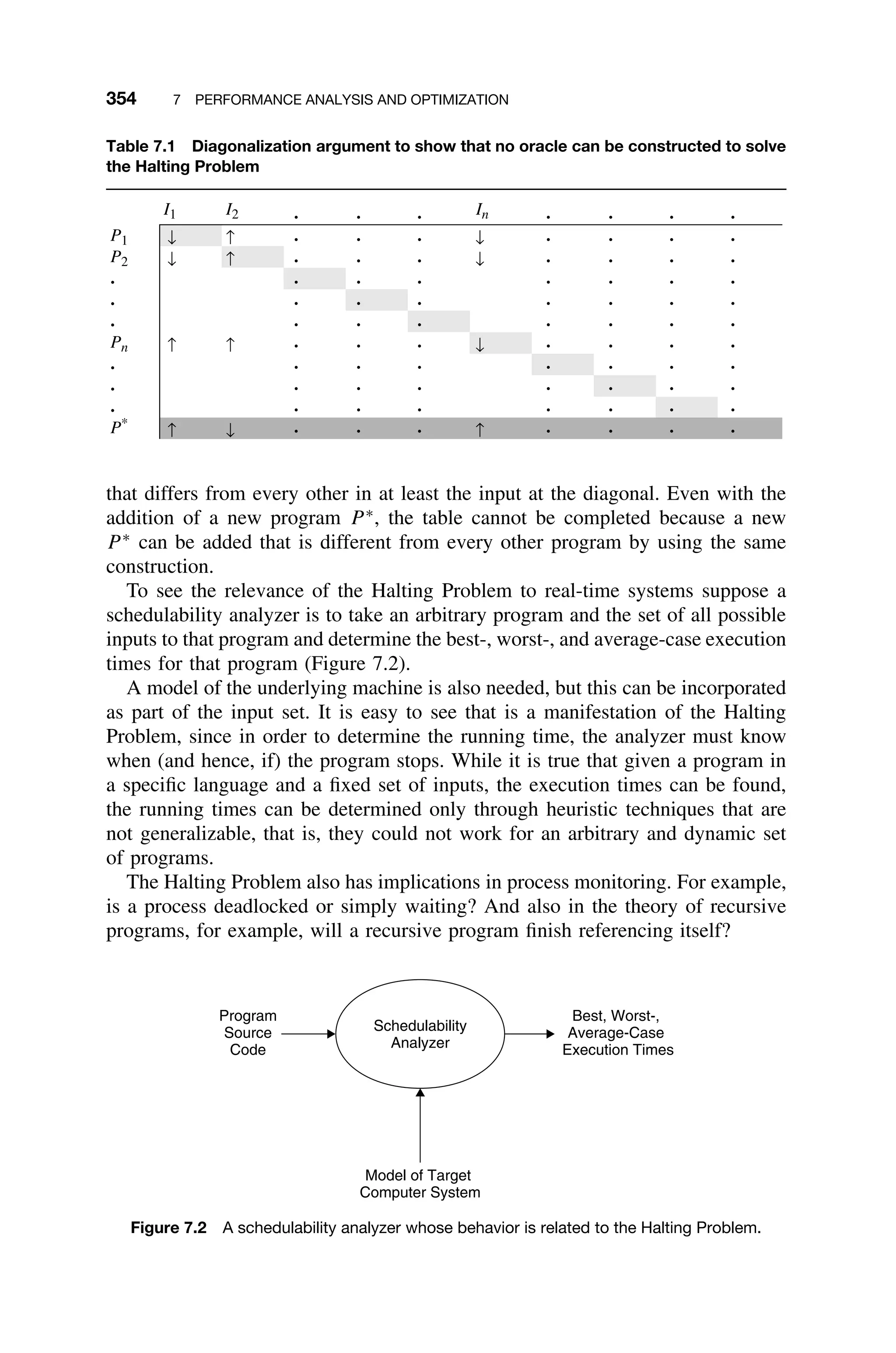
![7.1 THEORETICAL PRELIMINARIES 355
7.1.4 Amdahl’s Law
Amdahl’s Law is a statement regarding the level of parallelization that can be
achieved by a parallel computer [Amdahl67].2
Amdahl’s law states that for a
constant problem size, speedup approaches zero as the number of processor ele-
ments grows. It expresses a limit of parallelism in terms of speedup as a software
property, not a hardware one.
Formally, let n be the number of processors available for parallel processing.
Let s be the fraction of the code that is of a serial nature only, that is, it cannot
be parallelized. A simple reason why a portion of code cannot be parallelized
would be a sequence of operations, each depending on the result of the previous
operation. Clearly (1 − s) is the fraction of code that can be parallelized. The
speedup is then given as the ratio of the code before allocation to the parallel
processors to the ratio of that afterwards. That is,
Speedup =
s + (1 − s)
s +
(1 − s)
n
=
1
s +
(1 − s)
n
=
1
ns
n
+
(1 − s)
n
=
1
ns + 1 − s
n
=
n
ns + 1 − s
Hence,
Speedup =
n
1 + (n − 1)s
(7.1)
Clearly for s = 0 linear speedup can be obtained as a function of the num-
ber of processors. But for s 0, perfect speedup is not possible due to the
sequential component.
Amdahl’s Law is frequently cited as an argument against parallel systems and
massively parallel processors. For example, it is frequently suggested that “there
will always be a part of the computation which is inherently sequential, [and that]
2
Some of the following two sections has been adapted from Gilreath, W. and Laplante, P., Computer
Architecture: A Minimalist Perspective, Kluwer Academic Publishers, Dordrecht, The Netherlands,
2003 [Gilreath03].](https://image.slidesharecdn.com/epdf-230618090952-bdcb6616/75/epdf-pub_real-time-systems-design-and-analysis-pdf-378-2048.jpg)
![356 7 PERFORMANCE ANALYSIS AND OPTIMIZATION
no matter how much you speed up the remaining 90 percent, the computation
as a whole will never speed up by more than a factor of 10. The processors
working on the 90 percent that can be done in parallel will end up waiting for
the single processor to finish the sequential 10 percent of the task” [Hillis98].
But the argument is flawed. One underlying assumption of Amdahl’s law is that
the problem size is constant, and then at some point there is a diminishing margin
of return for speeding up the computation. Problem sizes, however, tend to scale
with the size of a parallel system. Parallel systems that are bigger in number of
processors are used to solve very large problems in science and mathematics.
Amdahl’s Law stymied the field of parallel and massively parallel computers,
creating an insoluble problem that limited the efficiency and application of par-
allelism to different problems. The skeptics of parallelism took Amdahl’s Law
as the insurmountable bottleneck to any kind of practical parallelism, which ulti-
mately impacted on real-time systems. However, later research provided new
insights into Amdahl’s Law and its relation to parallelism.
7.1.5 Gustafson’s Law
Gustafson demonstrated with a 1024-processor system that the basic presump-
tions in Amdahl’s Law are inappropriate for massive parallelism [Gustafson88].
Gustafson found that the underlying principle that “the problem size scales with
the number of processors, or with a more powerful processor, the problem
expands to make use of the increased facilities is inappropriate” [Gustafson88].
Gustafson’s empirical results demonstrated that the parallel or vector part of a
program scales with the problem size. Times for vector start-up, program loading,
serial bottlenecks, and I/O that make up the serial component of the run do not
grow with the problem size [Gustafson88].
Gustafson formulated that if the serial time, s, and parallel time, p = (1 − s),
on a parallel system with n processors, then a serial processor would require
the time:
s + p · n (7.2)
Comparing the plots of Equations 7.1 and 7.2 in Figure 7.3, it can be seen that
Gustafson presents a much more optimistic picture of speedup due to parallelism
than does Amdahl. Unlike the curve for Amdahl’s Law, Gustafson’s Law is a
simple line, “one with a much more moderate slope: 1 − n. It is thus much
easier to achieve parallel performance than is implied by Amdahl’s paradigm”
[Gustafson88].
A different take on the flaw of Amdahl’s Law can be observed as “a more
efficient way to use a parallel computer is to have each processor perform similar
work, but on a different section of the data. . . where large computations are con-
cerned this method works surprisingly well” [Hillis98]. Doing the same task but
on a different range of data circumvents an underlying presumption in Amdahl’s
Law, that is, “the assumption that a fixed portion of the computation. . . must be
sequential. This estimate sounds plausible, but it turns out not to be true of most
computations” [Hillis98].](https://image.slidesharecdn.com/epdf-230618090952-bdcb6616/75/epdf-pub_real-time-systems-design-and-analysis-pdf-379-2048.jpg)
![7.2 PERFORMANCE ANALYSIS 357
0
2
4
6
8
10
12
14
16
18
Number of Processors
Speedup
Amdahl
Gustafson
1 4 7 10 13 16 19 22 25
Figure 7.3 Linear speedup of Gustafson compared to ‘‘diminishing return’’ speedup of
Amdahl with 50% of code available for parallelization. Notice as number of processors increase,
speedup does not increase indefinitely for Amdahl due to serial component [Gilreath03].
7.2 PERFORMANCE ANALYSIS
It is natural to desire to analyze systems a priori to see if they will meet
their deadlines. Unfortunately, in a practical sense, this is rarely possible due
to the NP-completeness of most scheduling problems and constraints imposed
by synchronization mechanisms. Nonetheless, it is possible to get a handle on
the system’s behavior through analysis. The first step in performing any kind
of schedulability analysis is to determine, measure, or otherwise estimate the
execution of specific code units.
The need to know the execution time of various modules and the overall system
time-loading before implementation is important from both a management and
an engineering perspective. Not only are CPU utilization requirements stated as
specific design goals, but also knowing them a priori is important in selecting
hardware and the system design approach. During the coding and testing phases,
careful tracking of CPU utilization is needed to focus on those code units that
are slow or whose response times are inadequate. Several methods can be used
to predict or measure module execution time and CPU utilization.
7.2.1 Code Execution Time Estimation
Most measures of real-time performance require an execution-time estimate, ei,
for each task. The best method for measuring the execution time of completed
code is to use the logic analyzer that is described in Chapter 8. One advantage of
this approach is that hardware latencies and other delays are taken into account.
The drawback in using the logic analyzer is that the system must be completely
(or partially) coded and the target hardware available. Hence, the logic analyzer is
usually only employed in the late stages of coding, during testing, and especially
during system integration.](https://image.slidesharecdn.com/epdf-230618090952-bdcb6616/75/epdf-pub_real-time-systems-design-and-analysis-pdf-380-2048.jpg)
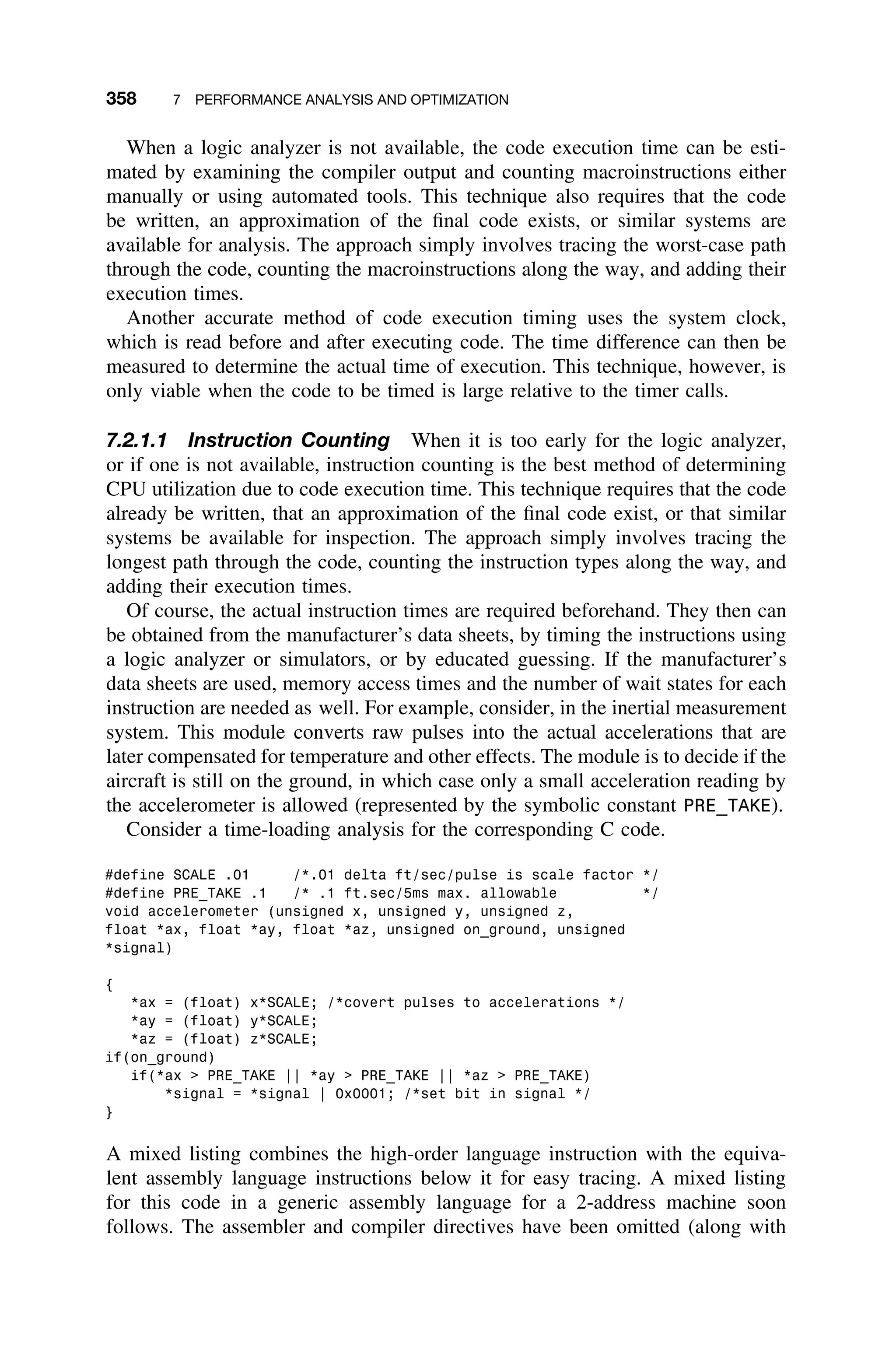
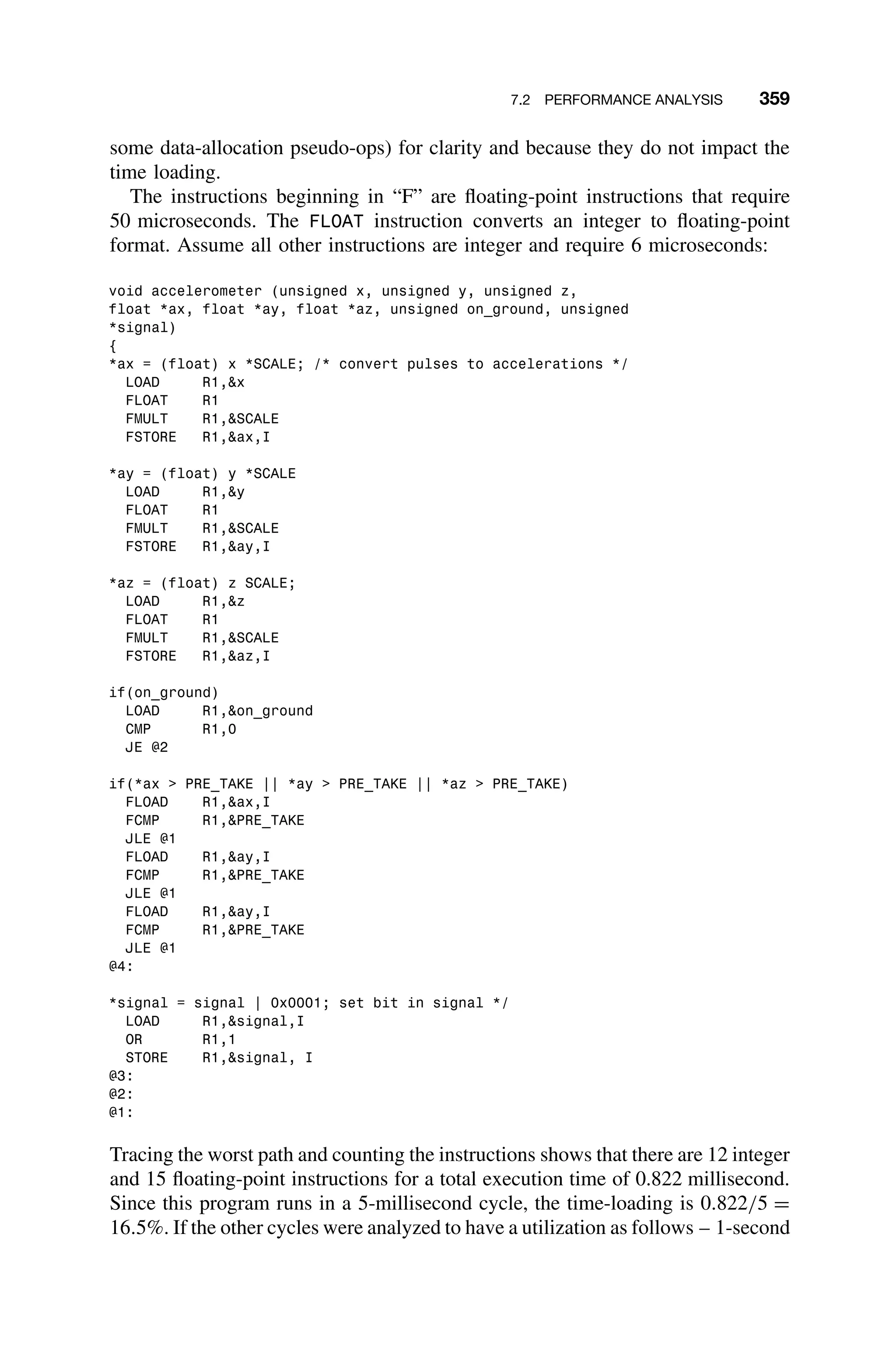
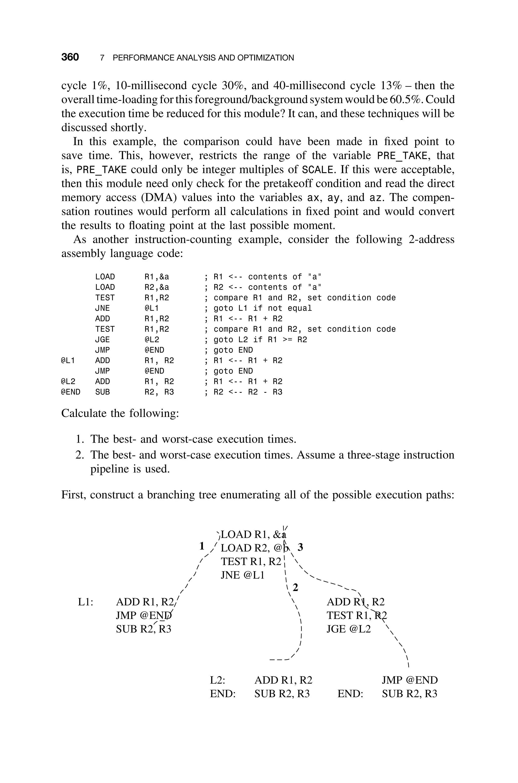
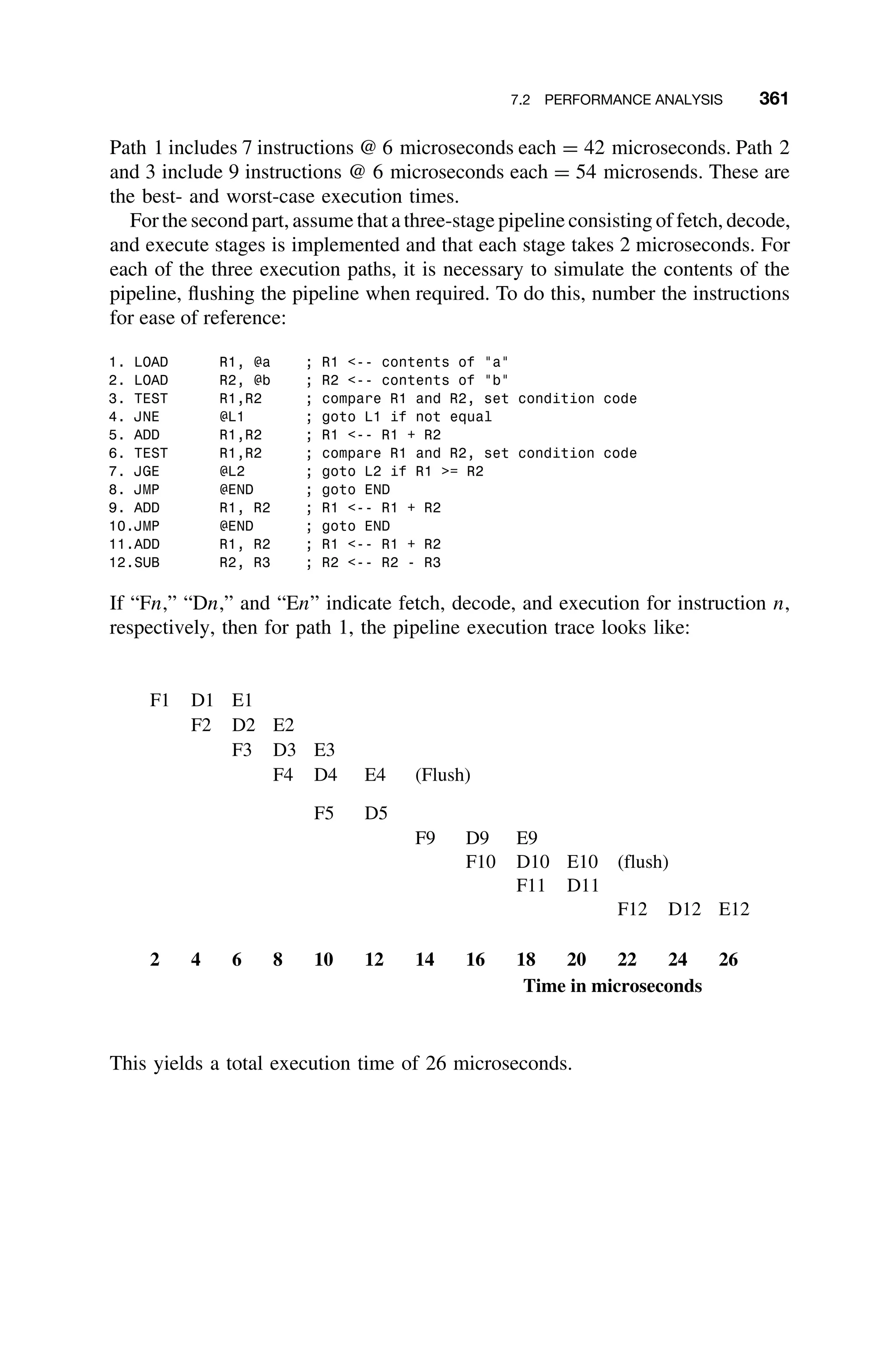
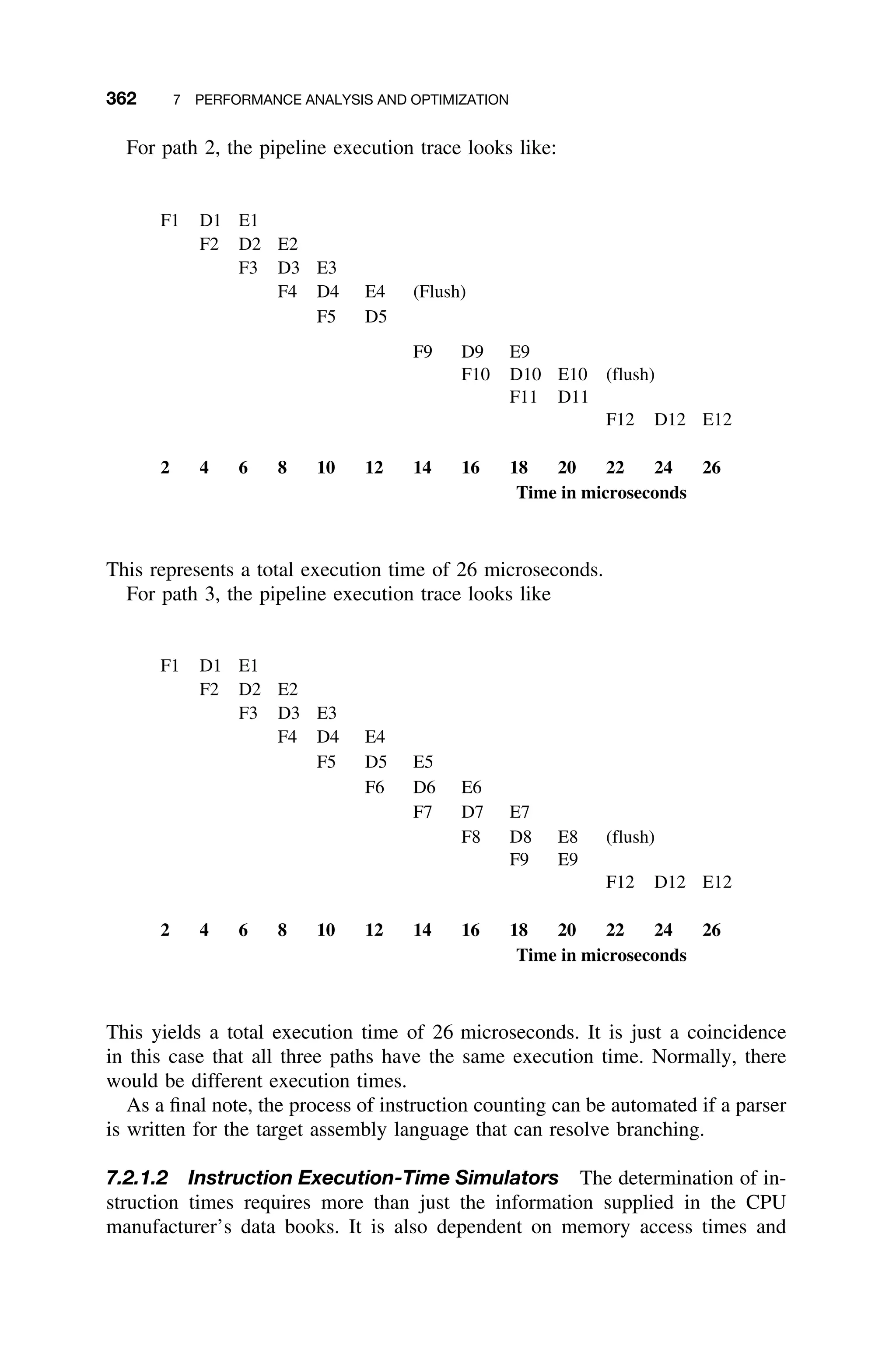
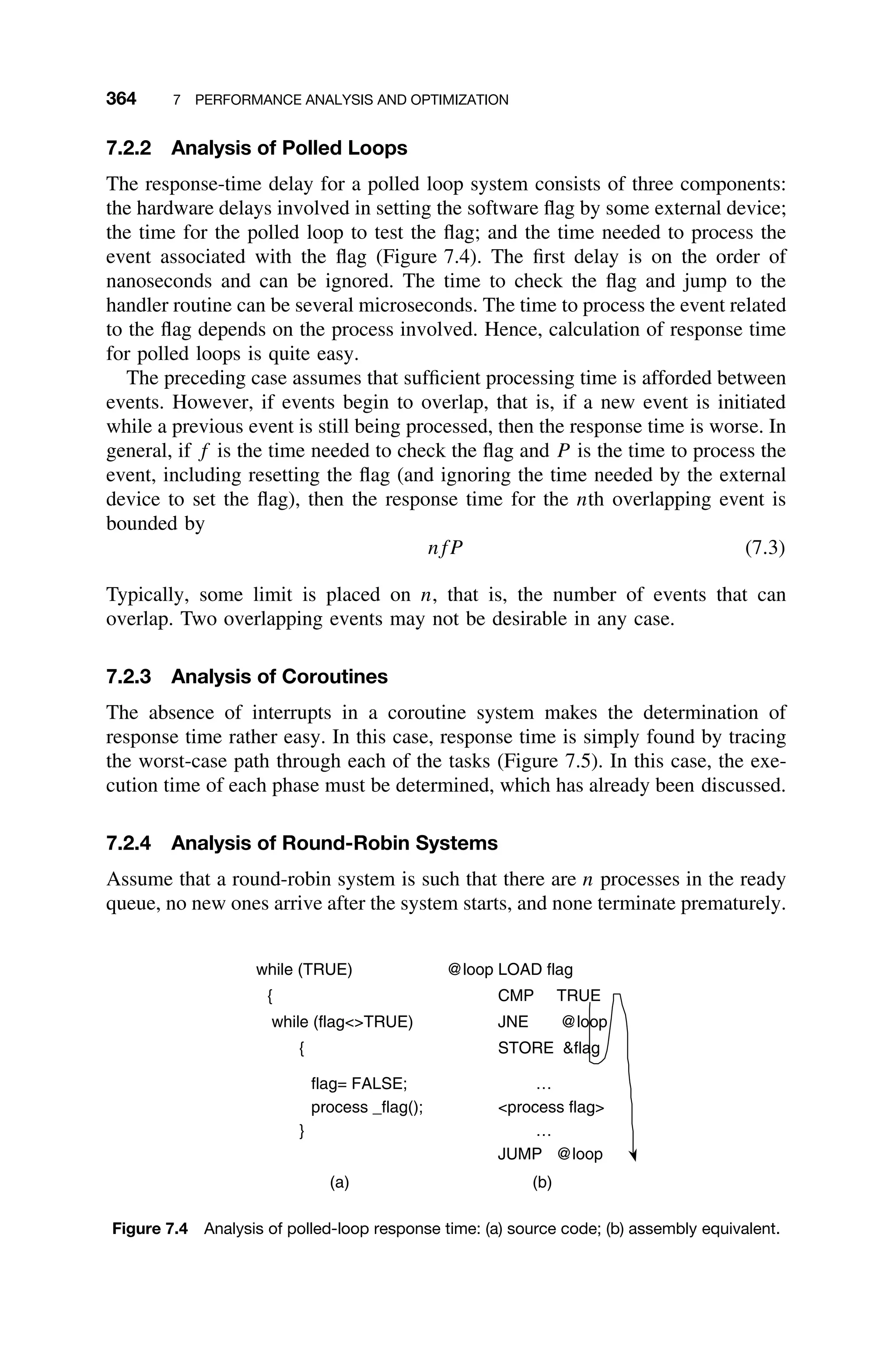
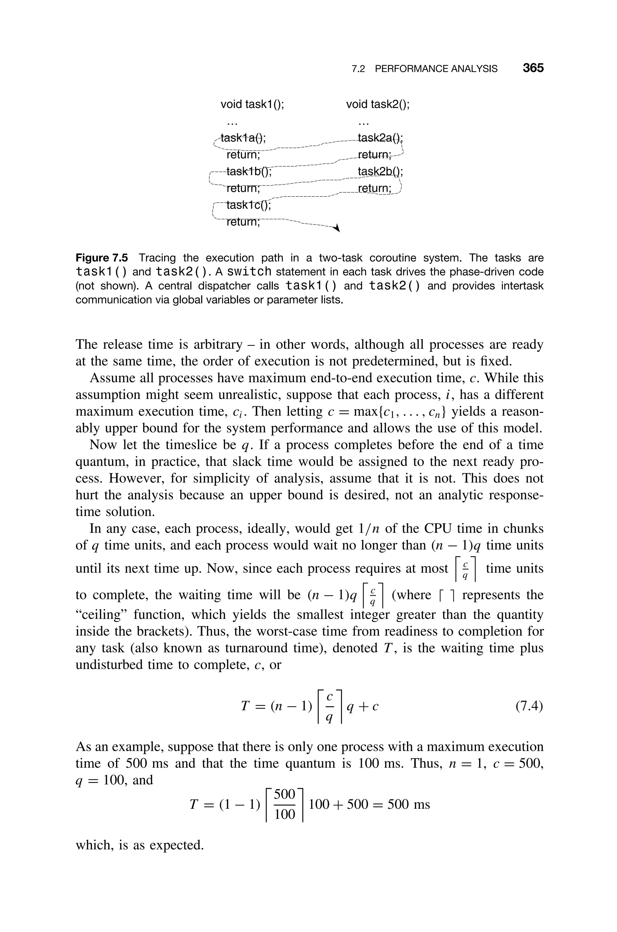
![366 7 PERFORMANCE ANALYSIS AND OPTIMIZATION
Now suppose there are five processes with a maximum execution time of
500 ms. The time quantum is 100 ms. Hence, n = 5, c = 500, q = 100, which
yields
T = (5 − 1)
500
100
100 + 500 = 2500 ms
This is intuitively pleasing, since it would be expected that five consecutive tasks
of 500 ms each would take 2500 ms end-to-end to complete.
However, now assume that there is a context switching overhead, o. Now each
process still waits no longer than (n − 1)q until its next time quantum, but there
is the additional overhead of n · o each time around for context switching. Again,
each process requires at most
c
q
time quanta to complete. So the worst-case
turnaround time for any task is now at most
T = [(n − 1)q + n · o]
c
q
+ c (7.5)
An assumption is that there is an initial context switch to load the first time around.
To illustrate, suppose that there is one process with a maximum execution time
of 500 ms. The time quantum is 40 ms and context switch time is 1 ms. Hence,
n = 1, c = 500, q = 40, o = 1. So,
T = [(1 − 1) · 40 + 1 · 1]
500
40
+ 500
= 1 · 13 + 500 = 513 ms
which is expected since the context switch time to handle the round-robin clock
interrupt costs 1 ms each time for the 13 times it occurs.
Next, suppose that there are six processes, each with a maximum execution
time of 600 ms, the time quantum is 40 ms, and context switch time costs 2 ms.
Now, n = 6, c = 600, q = 40, and o = 2. Then
T = [(6 − 1) · 40 + 6 · 2]
600
40
+ 600
= [5 · 40 + 10] · 15 + 600 = 3750 ms
which again is pleasing, because one would expect six processes of 600 ms in
duration to take at least 3600 ms, without context switching costs.
In terms of the time quantum, it is desirable that q c to achieve “fair”
behavior. For example, if q is very large, the round-robin algorithm is just the
first-come, first-served algorithm in that each process will execute to completion,
in order of arrival, within the very large time quantum.
The technique just discussed is also useful for cooperative multitasking analysis
or any kind of “fair” cyclic scheduling with context switching costs.](https://image.slidesharecdn.com/epdf-230618090952-bdcb6616/75/epdf-pub_real-time-systems-design-and-analysis-pdf-389-2048.jpg)
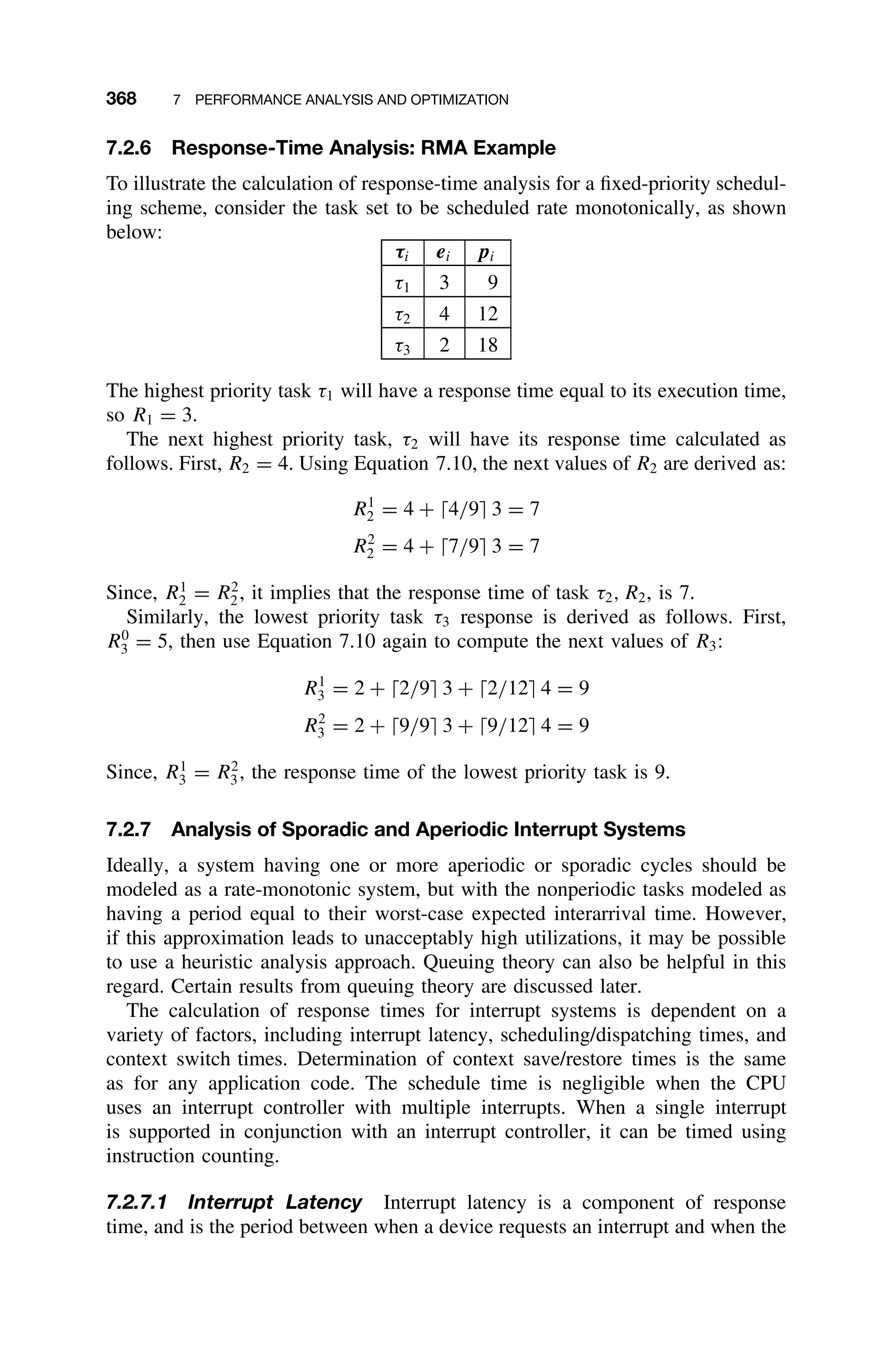
![370 7 PERFORMANCE ANALYSIS AND OPTIMIZATION
7.3 APPLICATION OF QUEUING THEORY
The classic queuing problem involves one or more producer processes called
servers and one or more consumer processes called customers. Queuing theory
has been applied to the analysis of real-time systems this way since the mid-
1960s (e.g., [Martin67]), yet it seems to have been forgotten in modern real-
time literature.
A standard notation for a queuing system is a three-tuple (e.g., M/M/1). The
first component describes the probability distribution for the time between arrivals
of customers, the second is the probability distribution of time needed to service
each customer, and the third is the number of servers. The letter M is customarily
used to represent exponentially distributed interarrival or service times.
In a real-time system, the first component of the tuple might be the arrival
time probability distribution for a certain interrupt request. The second com-
ponent would be the time needed to service that interrupt’s request,. The third
component would be unity for a single processing system and 1 for multipro-
cessing systems. Known properties of this queuing model can be used to predict
service times for tasks in a real-time system.
7.3.1 The M/M/1 Queue
The simplest queuing model is the M/M/1 queue, which represents a single-
server system with a Poisson arrival model (exponential interarrival times for
the customers or interrupt requests with mean 1/λ), and exponential service or
process time with mean 1/µ and λ µ . As suggested before, this model can be
used effectively to model certain aspects of real-time systems; it is also useful
because it is well known, and several important results are immediately available
[Kleinrock75]. For example, let N be the number of customers in the queue.
Letting ρ = λ/µ, then the average number of customers in the queue in such a
system is
N =
ρ
1 − ρ
(7.11)
with variance
σ2
N =
ρ
(1 − ρ)2
(7.12)
The average time a customer spends in the system is
T =
1/µ
1 − ρ
(7.13)
The random variable Y for the time spent in the system has probability distribu-
tion
s(y) = µ(1 − ρ)e−µ(1−ρ)y
(7.14)
with y ≥ 0.](https://image.slidesharecdn.com/epdf-230618090952-bdcb6616/75/epdf-pub_real-time-systems-design-and-analysis-pdf-393-2048.jpg)
![7.3 APPLICATION OF QUEUING THEORY 371
Finally, it can be shown that the probability that at least k customers are in
the queue is
P [≥ k in system] = ρk
(7.15)
In the M/M/1 model, the probability of exceeding a certain number of customers
in the system decreases geometrically. If interrupt requests are considered cus-
tomers in a certain system, then two such requests in the system at the same time
(a time-overloaded condition) have a far greater probability of occurrence than
three or more such requests. Thus, building systems that can tolerate a single
time-overload will contribute significantly to system reliability, while worrying
about multiple time-overload conditions is probably futile. The following sections
describe how the M/M/1 queue can be used in the analysis of real-time systems.
7.3.2 Service and Production Rates
Consider an M/M/1 system in which the customer represents an interrupt request
of a certain type and the server represents the processing required for that request.
In this single-processor model, waiters in the queue represent a time-overloaded
condition. Because of the nature of the arrival and processing times, this condition
could theoretically occur. Suppose, however, that the arrival or the processing
times can vary. Varying the arrival time, which is represented by the parameter λ,
could be accomplished by changing hardware or altering the process causing the
interrupt. Changing the processing time, represented by the parameter µ could
be achieved by optimization. In any case, fixing one of these two parameters,
and selecting the second parameter in such a way as to reduce the probability
that more than one interrupt will be in the system simultaneously, will ensure
that time-overloading cannot occur within a specific confidence interval.
For example, suppose 1/λ, the mean interarrival time between interrupt re-
quests, is known to be 10 milliseconds. It is desired to find the mean processing
time, 1/µ, necessary to guarantee that the probability of time overloading (more
than one interrupt request in the system) is less than 1%. Use Equation 7.15
as follows:
P [≥ 2 in system] =
λ
µ
2
≤ 0.01
or
1
µ
≤
0.01
λ2
then
⇒
1
µ
≤ 0.001 seconds
Thus, the mean processing time, 1/µ, should be no more than 1 millisecond to
guarantee with 99% confidence that time overloading cannot occur.
As another example, suppose the service time, 1/µ, is known to be 5 millisec-
onds. It is desired to find the average arrival time (interrupt rate), 1/λ, to guarantee](https://image.slidesharecdn.com/epdf-230618090952-bdcb6616/75/epdf-pub_real-time-systems-design-and-analysis-pdf-394-2048.jpg)
![7.3 APPLICATION OF QUEUING THEORY 373
the exponential function with mean 1/λ = 5 milliseconds. A process handles the
data in an amount of time determined by the exponential function with mean
1/µ = 3 milliseconds. The mean response time for this interrupt request is seen
from Equation 7.13 to be:
T =
3
1 −
1/5
1/3
= 7.5 milliseconds
A probability distribution for the random variable determining the mean response
time can be found by using Equation 7.14. Omitting context switching and inter-
task interference gives
s(t) =
1
3
1 −
3
5
e−(1/3)(1−(3/5))t
or
s(t) =
2
5
e−(2/15)t
Note that the response time will be deleteriously affected if the interrupt rate is
greater than the mean service rate.
7.3.5 Other Results from Queuing Theory
The M/M/1 queue can be used in a variety of other ways to model real-time
systems. The only requirements are that the producer be modeled as a Pois-
son process and that the consumption time be exponential. Although the model
assumes an infinite-length queue, confidence intervals can be fixed for modeling
realistic finite-sized queues.
Systems that can be modeled to match other queuing system models can benefit
from the well-known results there. For example, the M/M/1 queue with Poisson
arrival (exponential interarrival) and general service time probability distributions
can be used. Other results cover the general arrival and service densities. Rela-
tionships involving balking customers, those that leave the queue, can be used
to represent rejected spurious interrupts or time overloads.
7.3.6 Little’s Law
An important result in queuing theory, Little’s Law, has some application in
real-time system performance prediction. Little’s Law, which appeared in 1961,
states that the average number of customers in a queuing system, Nav, is equal
to the average arrival rate of the customers to that system, rav, times the average
time spent in that system, tav [Kleinrock75]:
Nav = ravtav (7.16)](https://image.slidesharecdn.com/epdf-230618090952-bdcb6616/75/epdf-pub_real-time-systems-design-and-analysis-pdf-396-2048.jpg)
![374 7 PERFORMANCE ANALYSIS AND OPTIMIZATION
If n servers are present, then
Nav =
n
i=1
ri,avti,av (7.17)
where ri,av is the average arrival rate for customers to server i, and ti,av is the
average service time for server i.
Viewing each process as a server and interrupt arrivals as customers, Little’s
Law is Equation 1.2 for CPU utilization with ei = ti,av and 1/pi = ri,av. For
example, a system is known to have periodic interrupts occurring at 10, 20, and
100 milliseconds and a sporadic interrupt that is known to occur on average
every 1 second. The average processing time for these interrupts is 3, 8, 25, and
30 milliseconds. Then by Little’s Law the average number of customers in the
queue is
Nav = (1/10)3 + (1/20)8 + (1/100)25 + (1/1000)30 = 0.98
This result is the same one obtained by using Equation 1.2 for CPU utilization.
7.3.7 Erlang’s Formula
Another useful result of queuing theory is Erlang’s Loss Formula. Suppose there
are m servers (or processes) and arriving customers (interrupts). Each newly
arriving interrupt is serviced by a process, unless all servers are busy (a potential
time-overloaded condition). In this, case the customer (interrupt) is lost. If it
is assumed that the average service (process) time is µ and the average arrival
time (interrupt rate) is λ, then the fraction of time that all servers are busy (a
time-overloaded condition) is given by
p =
(λ/µ)m
/m!
m
k=0(λ/µ)k/k!
(7.18)
This result dates back to 1917 [Kleinrock75].
Applying Erlang’s Formula to the previous example gives m = 4, λ = 380,
and µ = 16.5; then
p =
(380/16.5)4
/4!
1 + (380/16.5) + (380/16.5)2/2 + (380/16.5)3/3! + (380/16.5)4/4!
= 0.834
This means there is a potential for time overloading 83.4% of the time. Based
on the average time-loading figure of 98% and the rate-monotonic theorem, this
seems reasonable.](https://image.slidesharecdn.com/epdf-230618090952-bdcb6616/75/epdf-pub_real-time-systems-design-and-analysis-pdf-397-2048.jpg)
![376 7 PERFORMANCE ANALYSIS AND OPTIMIZATION
buffer in the previous cases will take 11 seconds – sufficient time before the
next expected burst. If bursts occur too frequently, then buffer overflow will
occur. In this case the system is unstable, and either upgrading the processor or
downgrading the production process is necessary to solve the problem.
7.4.2 Variable Buffer-Size Calculation
It is often not accurate to assume that burst periods are fixed; they will frequently
be variable. Suppose that a process produces data at a rate given by the real-
valued function p(t). Also suppose that another task consumes or uses the data
produced by the first task at a rate determined by the real-valued function c(t).
The data are produced during a burst period T = t1 − t2, where t1 t2 represent
the start and finish times of the burst. Then the buffer size needed at time t2 can
be expressed as
B(t2) =
t2
t1
[p(t) − c(t)] dt (7.20)
Note that when p(t) and c(t) are constant, Equation 7.20 becomes Equation 7.19
(see Exercise 7.9). For example, a task produces data at a rate (in bytes per
second) that is determined by the function:
p(t) =
10,000t 0 ≤ t ≤ 1
10,000(t − 2) 1 t ≤ 2
0 elsewhere
with t representing the burst period. The data are consumed by a task at a rate
determined by the function:
c(t) =
10,000(1/4)t 0 ≤ t ≤ 2
10,000(1 − 1/4t) 2 t ≤ 4
0 elsewhere
If the burst period is known to be 1.6 seconds, what is the necessary buffer size?
Using Equation 7.20 yields,
B(1.6) =
1.6
0
[p(t) − c(t)] dt
= 10,000
1
0
[(t − 1/4t)] dt + 10,000
1.6
1
[(2 − t) − 1/4t] dt
= 10,000(3/4)
1
0
t dt +
1.6
1
dt − 10,000(5/4)
1.6
1
t dt
= 10,000(3/8)t2
1
0
+ 10,000(2)t
1.6
1
− 10,000(5/8)t2
1.6
1
= 10,000(3/8) + 10,000(3.2 − 2) − 10,000(5/8)(2.56 − 1)
≈ 600 bytes](https://image.slidesharecdn.com/epdf-230618090952-bdcb6616/75/epdf-pub_real-time-systems-design-and-analysis-pdf-399-2048.jpg)
![7.5 PERFORMANCE OPTIMIZATION 377
If the burst period is determined by the real-valued function u(t), then for a burst
starting at time t1 and ending at t2 the necessary buffer size is
B(t) =
u(t1)
t1
[p(t) − c(t)] dt (7.21)
In the previous example, if the burst starts at a time determined by the Gaussian
distribution
u(t) =
1
√
2π
e−(t−2)2
/2
(7.22)
at time t = 0, then it is will end at time u(0) = 0.053991. Recalculation of the
buffer size now yields
B(0.053991) =
0.053991
0
[p(t) − c(t)] dt
= 10,000
0.053991
0
[t − 1/4t] dt
= 10,000(3/4)
0.053991
0
t dt
= 10,000(3/8)t2
0.053991
0
= 10,000(3/8)[0.002915]
≈ 11 bytes
7.5 PERFORMANCE OPTIMIZATION
Identifying wasteful computation is a preliminary step in reducing code execu-
tion time, and hence, CPU utilization. Many approaches employed in compiler
optimization can be used, but other methods have evolved that are specifically
oriented toward real-time systems.
7.5.1 Compute at Slowest Cycle
All processing should be done at the slowest rate that can be tolerated. Checking
a discrete temperature for a large room at faster than 1 second may be wasteful,
for temperature typically cannot change quickly owing to thermal inertia. In the
nuclear plant example, a dedicated sensor is used to monitor the temperature,
which then issues a high-level priority if any overtemperature is detected.
7.5.2 Scaled Numbers
In virtually all computers, integer operations are faster than floating-point ones.
This fact can be exploited by converting floating-point algorithms into scaled](https://image.slidesharecdn.com/epdf-230618090952-bdcb6616/75/epdf-pub_real-time-systems-design-and-analysis-pdf-400-2048.jpg)
![378 7 PERFORMANCE ANALYSIS AND OPTIMIZATION
integer algorithms. In these so-called scaled numbers, the least significant bit
(LSB) of an integer variable is assigned a real number scale factor. Scaled
numbers can be added and subtracted together and multiplied and divided by
a constant (but not another scaled number). The results are converted to float-
ing point only at the last step, thus saving considerable time. For example,
suppose an analog-to-digital (A/D) converter is converting accelerometer data.
If the least significant bit of the two’s complement 16-bit integer has value
0.0000153 ft/s2
, then any acceleration can be represented up to the maximum
value of (215
− 1)∗
0.0000153 = 0.5013351 ft/s2
. The 16-bit number 0000 0000
0001 011, for example, represents an acceleration of 0.0001683 ft/s2
.
A common practice is to quickly convert the integer number into its floating-
point equivalent by xf = x · 0.0000153 and then proceed to use it in calculations
directly with other converted numbers; for example, diff = xf − zf , where zf
is a similarly converted floating-point number. Instead, the calculation can be
performed in integer form first and then converted to floating point: diff = (x −
z) · 0.0000153.
For applications involving the numerous addition and subtraction of like data,
scaled numbers can introduce significant savings. Note, however, that multipli-
cation and division by another scaled number cannot be performed on a scaled
number as those operations change the scale factor. Finally, accuracy is generally
sacrificed by excessive use of scaled numbers.
7.5.3 Binary Angular Measure
Another type of scaled number is based on the property that adding 180◦
to any
angle is analogous to taking its two’s complement. This technique, called binary
angular measurement (BAM) works as follows. Consider the LSB of an n-bit
word to be 2n−1
· 180 degrees with the most significant bit (MSB) = 180 degrees.
The range of any angle θ represented this way is 0 ≤ θ ≤ 360 − 180 · 2−(n−1)
degrees. A 16-bit BAM word is shown in Figure 7.6. For more accuracy, BAM
can be extended to two more words. Each n-bit word has a maximum value of
2n
− 2−(n−1)
· 180
◦
= 360
◦
− LSB (7.23)
with granularity
2−(n−1)
· 180
◦
= LSB (7.24)
Consider the 16-bit BAM word:
0000 0000 10100 110
Its binary angular measurement is 166 · 180◦
· 2−15
= 0.9118◦
.
180 90 45 22.5 180·2−14
180·2−15
… … … … … … … … … …
Figure 7.6 A 16-bit binary angular measurement word [Laplante03c].](https://image.slidesharecdn.com/epdf-230618090952-bdcb6616/75/epdf-pub_real-time-systems-design-and-analysis-pdf-401-2048.jpg)
![7.5 PERFORMANCE OPTIMIZATION 379
BAM can be added and subtracted together and multiplied and divided by
constants as if they were unsigned integers, and converted at the last stage to
produce floating-point results. It is easy to show that the overflow condition for
BAM numbers presents no problem as the angle simply wraps around to 0. BAM
is frequently used in navigation software, robotic control, and in conjunction with
digitizing imaging devices.
7.5.4 Look-Up Tables
Another variation of the scaled-number concept uses a stored table of function
values at fixed intervals. Such a table, called a look-up table, allows for the
computation of continuous functions using mostly fixed-point arithmetic.
Let f (x) be a continuous real function and let x be the interval size. Suppose
it is desired to store n values of f over the range [x0, x0 + (n − 1) x] in an array
of scaled integers. Values for the derivative, f
may also be stored in the table.
The choice of x represents a trade-off between the size of the table and the
desired resolution of the function. A generic look-up table is given in Table 7.2.
It is well known that the table can be used for the interpolation of x x̂
x + x by the formula:
f (x̂) = f (x) + (x̂ − x)
f (x + x) − f (x)
x
(7.25)
This calculation is done using integer instructions except for the final multipli-
cation by the factor (x̂ − x)/ x and conversion to floating point. As a bonus,
the look-up table has faster execution time if x̂ happens to be one of the table
values. If f
(x) is also stored in the table, then the look-up formula becomes:
f (x̂) = f (x) + (x̂ − x)f
(x) (7.26)
This improves the execution time of the interpolation somewhat.
The main advantage in using look-up tables, of course, is speed. If a table value
is found and no interpolation is needed, then the algorithm is much faster than the
corresponding series expansion. In addition, even if interpolation is necessary,
Table 7.2 A generic function look-up table
x f (x)
x0 f (x0)
x0 + x f (x0 + x)
x0 + 2 x f (x0 + 2 x)
.
.
.
.
.
.
x0 + (n − 1) x f (x0 + (n − 1) x)](https://image.slidesharecdn.com/epdf-230618090952-bdcb6616/75/epdf-pub_real-time-systems-design-and-analysis-pdf-402-2048.jpg)
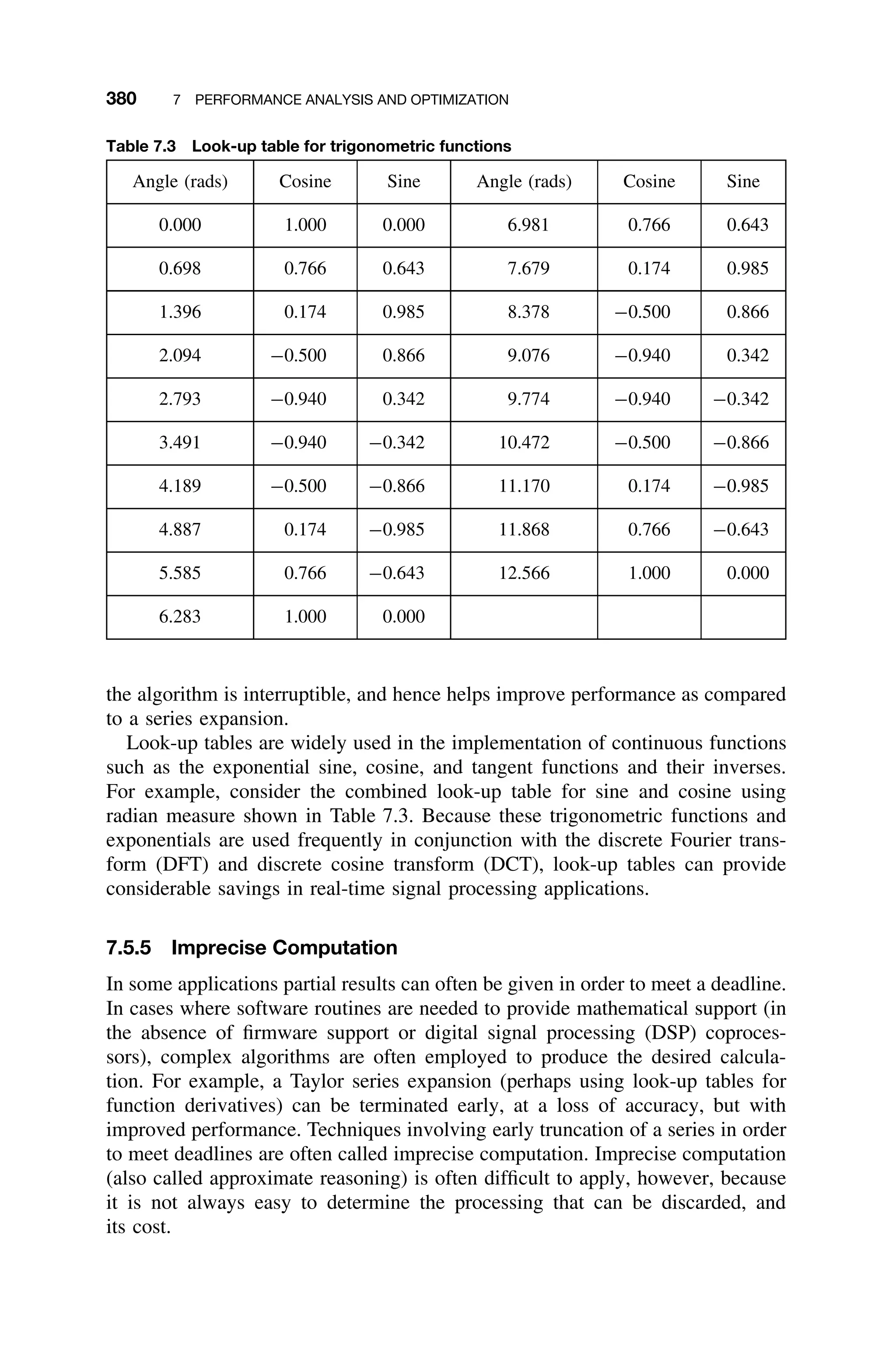
![384 7 PERFORMANCE ANALYSIS AND OPTIMIZATION
the optimization explicitly. And although the original statement may be more
descriptive, a comment can be provided to explain the optimized statement.
For example, if the program uses π/2 it should be precomputed during the
initialization and stored as a constant named, for example, pi_div_2. This
will typically save one floating-point load and one floating-point divide instruc-
tion – potentially tens of microseconds. In a 5-millisecond real-time cycle, this
can lead to time-loading savings of 0.1%. Incidentally, using this strategy again
illustrates the inverse relationship between time and memory utilization: code
execution time has been reduced, but extra memory is needed to store the pre-
computed constant.
7.6.6 Loop Invariant Optimization
Most compilers will move computations outside loops that do not need to be per-
formed with the loop, a process called loop invariant optimization. For example,
consider the following code fragment in C:
x=100;
while (x0)
x = x-y+z;
it can be replaced by
x=100;
t=y+z;
while(x0)
x=x-t;
This moves an instruction outside the loop, but requires additional memory.
7.6.7 Loop Induction Elimination
A variable i is called an induction variable of a loop if every time i changes
its value, and it is incremented or decremented by some constant. A common
situation is one in which the induction variable is i and another variable, j,
which is a linear function if it, is used to offset into some array. Often i is used
only for a test of loop termination. Variable i can be eliminated by replacing its
test for one on j. For example, consider the following C program fragment:
for (i=1,i=10;i++)
a [i+1] = 1;
an optimized version is
for (i=2,i=11;i++)
a[j] = 1;
eliminating the extra addition within the loop.](https://image.slidesharecdn.com/epdf-230618090952-bdcb6616/75/epdf-pub_real-time-systems-design-and-analysis-pdf-407-2048.jpg)
![388 7 PERFORMANCE ANALYSIS AND OPTIMIZATION
for(i=1;i=6;i++)
a[i] = a[i]*8;
is replaced by
a[1]=a[1]*8;
a[2]=a[2]*8;
a[3]=a[3]*8;
a[4]=a[4]*8;
a[5]=a[5]*8;
a[6]=a[6]*8;
A less dramatic version reduces the loop overhead by a factor of 3:
for (i=1;i=6;i+3)
{
a[i]=a[i]*8;
a[i+1]=a[i+1]*8;
a[i+2]=a[i+2]*8;
};
7.6.16 Loop Jamming
Loop jamming or loop fusion is a technique for combining two similar loops into
one, thus reducing loop overhead by a factor of 2. For example, the following
C code:
for (i=1;i=100;i++)
x[i]=y[i]*8;
for (i=1;i=100;i++)
z[i]=x[i]*y[i];
can be replaced by
for (i=1;i=100;i++)
{
x[i]=y[i]*8;
z[i]=x[i]*y[i];
};
7.6.16.1 Cross-Jump Elimination If the same code appears in more than
one case in a case or switch statement, then it is better to combine the cases
into one. This eliminates an additional jump or cross jump. For example, the
following code :
switch (x)
{
case 0: x=x+1;
break;
case 1: x=x*2;
break;](https://image.slidesharecdn.com/epdf-230618090952-bdcb6616/75/epdf-pub_real-time-systems-design-and-analysis-pdf-411-2048.jpg)
![7.6 RESULTS FROM COMPILER OPTIMIZATION 389
case 2: x=x+1;
break;
case 3: x=2;
break;
};
can be replaced by
switch (x)
{
case 0:
case 2: x=x+1;
break;
case 1: x=x*2;
break;
case 3: x=2;
break;
};
7.6.17 More Optimization Techniques
A sampling of other optimization considerations follows [Jain91]. Note that
in most cases these techniques will optimize the average case, not the worst
case.
ž Optimize the common case. The most frequently used path should also be
the most efficient. For example, arrange a series of IF statements so that the
most likely value is tested first. Similarly, arrange a series of AND conditions
so that the condition most likely to fail is tested first. Likewise, arrange OR
conditions so the most likely to succeed is tested first. This technique is
called Boolean short-circuiting.
ž Arrange entries in a table so that the most frequently sought values are the
first to be compared (this is just a variation of the preceding).
ž Replace threshold tests on monotone (continuously nondecreasing or nonin-
creasing) functions by tests on their parameters, thereby avoiding evaluation
of the function. For example, if exp(x) is a function computing ex
, then
instead of using:
if (exp(x) exp(y)) then . . .
use:
if (x y) then . . .
which will save two evaluations of the costly function exp(x).
ž Link the most frequently used procedures together to maximize the locality
of the reference (this only applies in paging or cached systems).
ž Store redundant data elements to increase the locality of reference. This
technique only applies in paging or cached systems.](https://image.slidesharecdn.com/epdf-230618090952-bdcb6616/75/epdf-pub_real-time-systems-design-and-analysis-pdf-412-2048.jpg)
![390 7 PERFORMANCE ANALYSIS AND OPTIMIZATION
ž Store procedures in memory in sequence so that calling and called sub-
routines (procedures) will be loaded together to increase the locality of
reference. Again, this only applies in paging or cached systems.
7.6.18 Combination Effects
Although many of the optimization techniques discussed can be automated, most
compilers only perform one optimization pass, overlooking opportunities that are
not revealed until after at least one pass. Hence, hand optimization can provide
additional execution time savings. To see the effects of multiple-pass optimiza-
tion, consider the following example. The C code fragment:
for (j=1;i=3;j++)
{
a[j]=0;
a[j]=a[j]+2*x
};
for (k=1;k=3;k++)
b[k]=b[k]+a[k]+2*k*k;
is improved by loop jamming, loop invariant removal, and removal of extraneous
code (in this case the initialization of a[j]). The resultant code is:
t=2*x;
for (j=1;j=3;j++)
{
a[j]=t;
b[j]=b[j]+a[j]+2*j*j;
};
Next, loop unrolling yields:
t=2*x;
a[1]=t ;
b[1]=b[1]+a[1]+2*1*1;
a[2]=t ;
b[2]=b[2]+a[2]+2*2*2;
a[3]=t ;
b[3]=b[3]+a[3]+2*3*3;
Finally, after constant folding, the improved code is
t=2*x;
a[1]=t;
b[1]=b[1]+a[1]+2;
a[2]=t;
b[2]=b[2]+a[2]+8;
a[3]=t;
The original code involved nine additions and nine multiplications, numerous
data movement instructions, and loop overheads. The improved code requires
only six additions, 1 multiplication, less data movement, and no loop overhead.](https://image.slidesharecdn.com/epdf-230618090952-bdcb6616/75/epdf-pub_real-time-systems-design-and-analysis-pdf-413-2048.jpg)
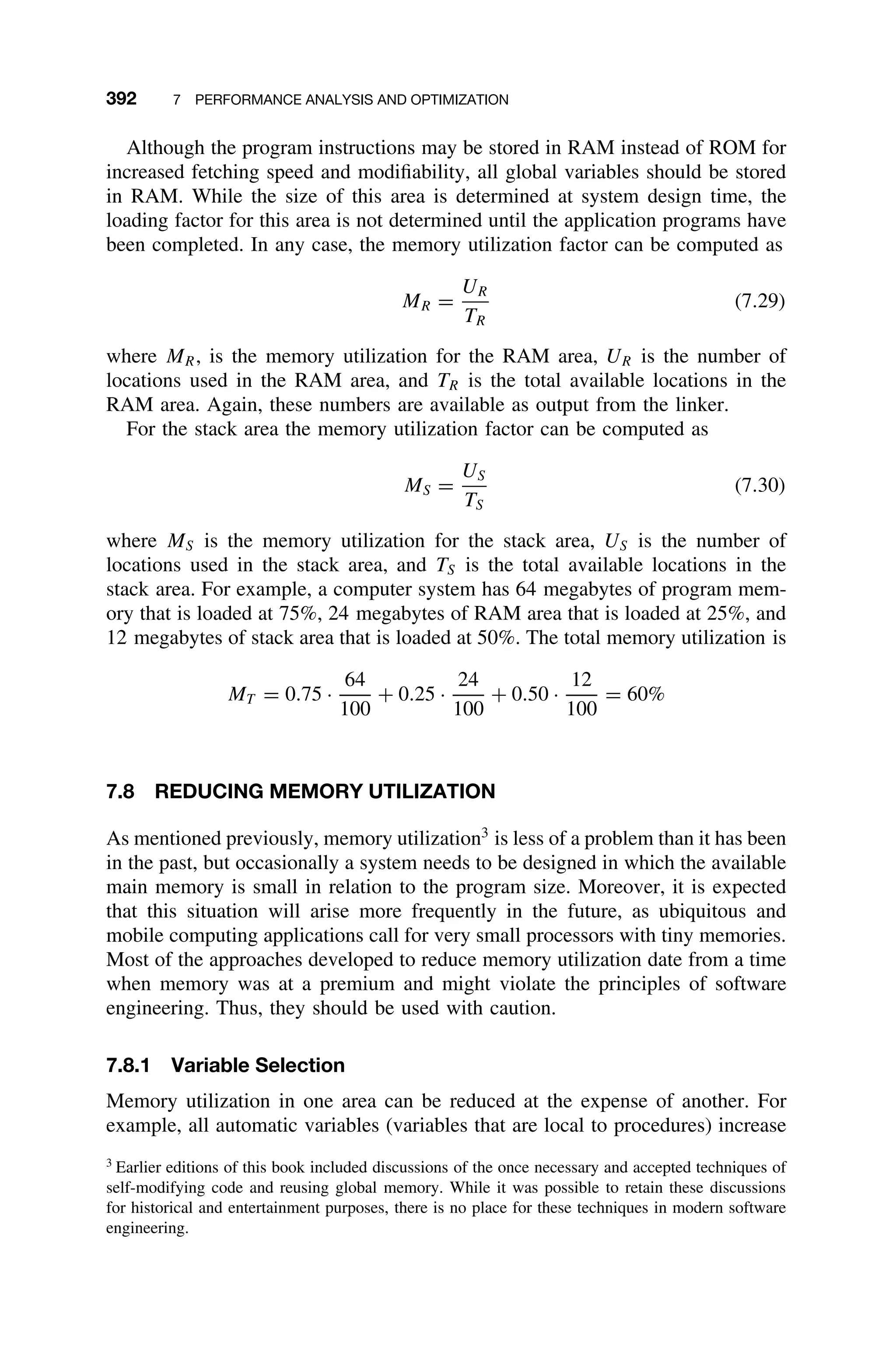
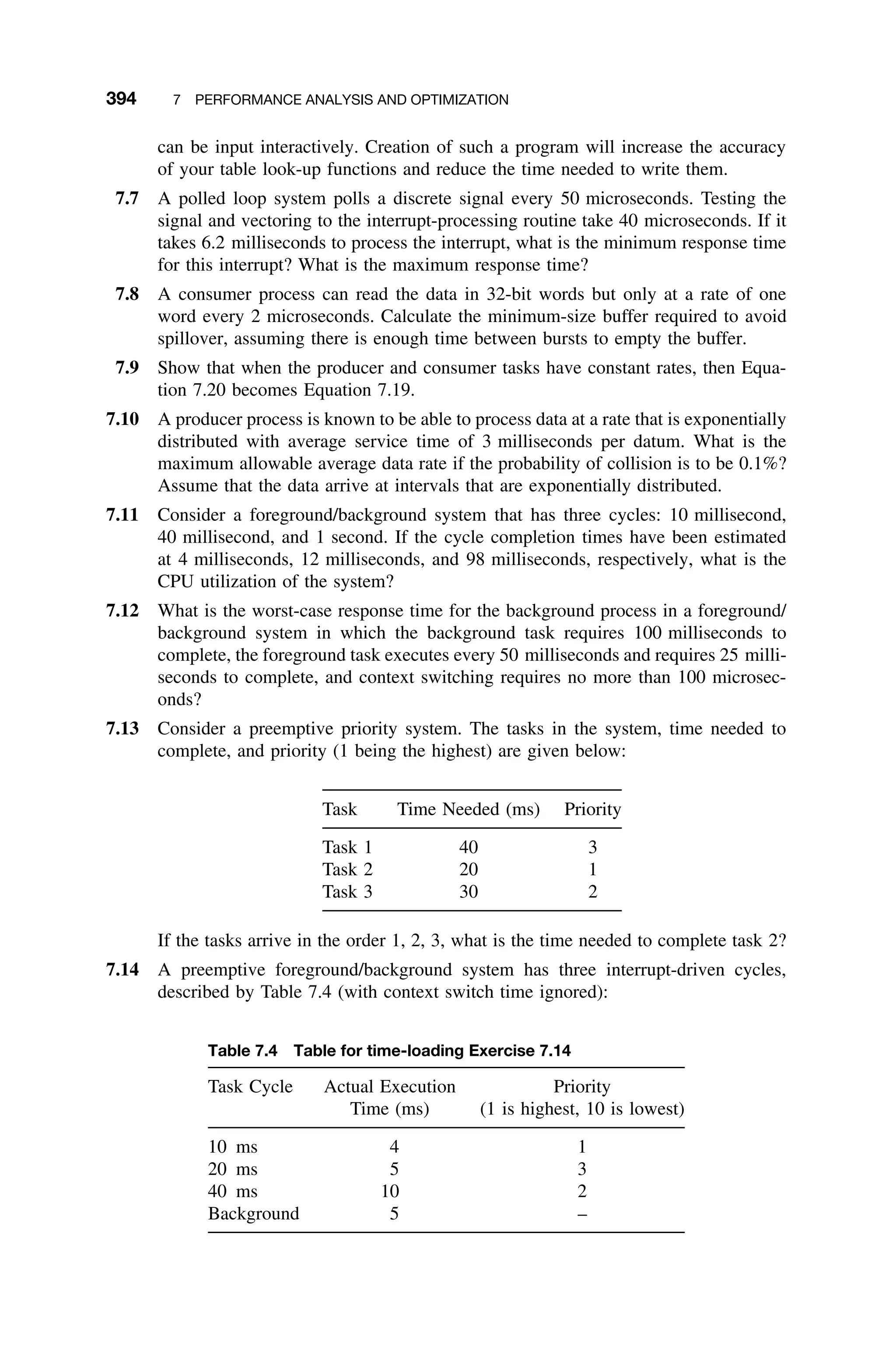
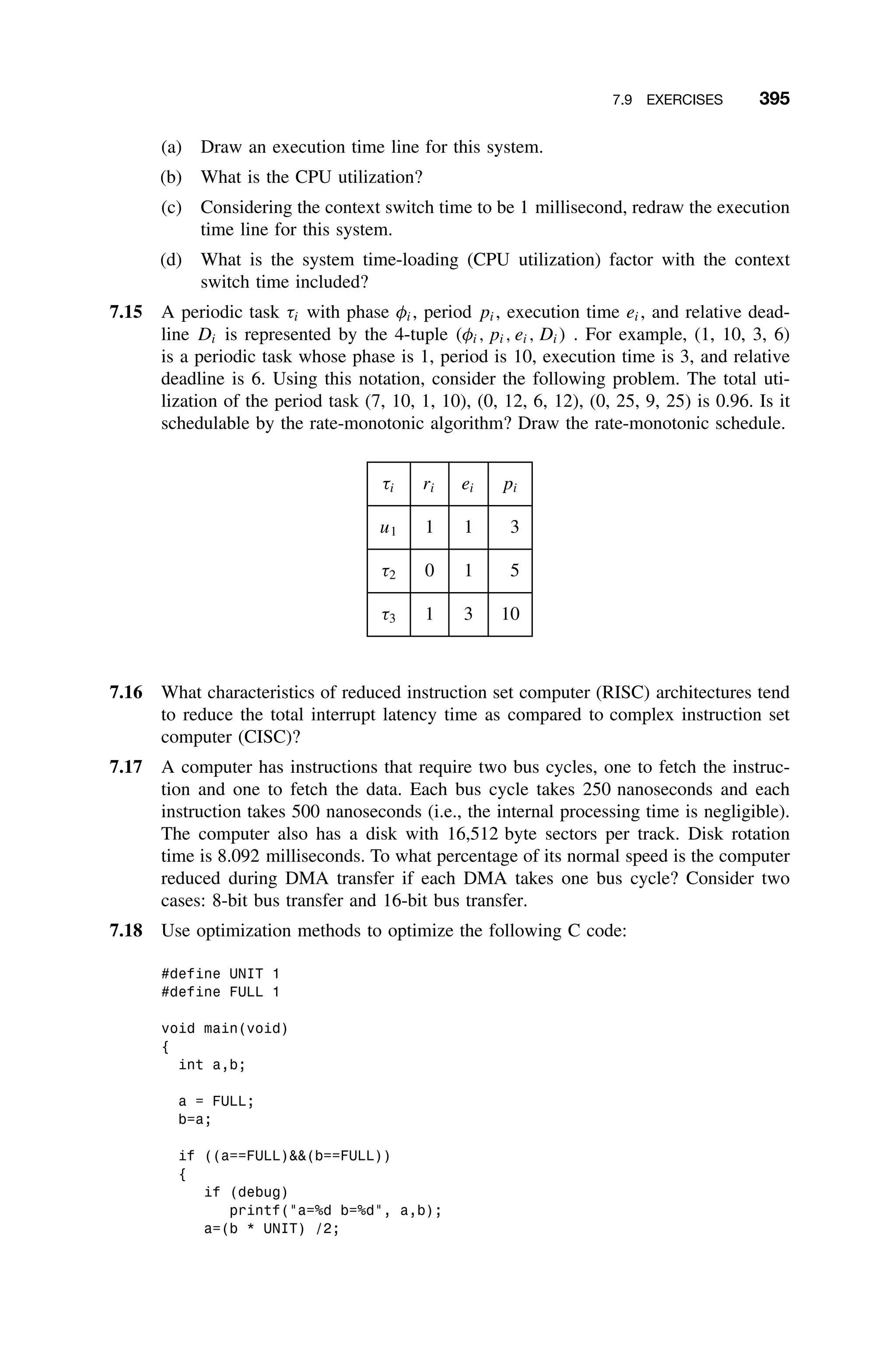
![398 8 ENGINEERING CONSIDERATIONS
noncommented source-code statements (NCSS). That is, the number of executable
program instructions, excluding comment statements, header files, formatting
statements, macros, and anything that does not show up as executable code after
compilation or cause allocation of memory, are counted. Another related metric
is source lines of code (SLOC), the major difference being that a single source
line of code may span several lines. For example, an if-then-else statement
would be a single SLOC, but multiple delivered source instructions.
While the clock metric essentially measures the weight of a printout of the
source code, thinking in these terms makes it likely that the usefulness of KLOC
will be unjustifiably dismissed as supercilious. But is it not likely that 1000 lines
of code is going to have more errors than 100 lines of code? Would it not take
longer to develop the latter than the former? Of course, the answer is dependent
on how complex the code is.
One of the main disadvantages of using lines of source code as a metric is that
it can only be measured after the code has been written. While it can be esti-
mated beforehand and during software production based on similar projects, this
is far less accurate than measuring the code after the fact. Nevertheless, KLOC
is a useful metric, and in many cases is better than measuring nothing. Moreover
many other metrics are fundamentally based on lines of code. For example, a
closely related metric is delta KLOC. Delta KLOC measures how many lines
of code change over some period of time. Such a measure is useful, perhaps,
in the sense that as a project nears the end of code development, Delta KLOC
would be expected to be small. Other, more substantial metrics are also derived
from KLOC.
8.1.2 McCabe’s Metric
A valid criticism of the KLOC metric is that it does not take into account
the complexity of the software involved. For example, one thousand lines of
print statements probably has fewer defects than one hundred lines of a real-
time kernel.
To attempt to measure software complexity, cyclomatic complexity was intro-
duced to measure program flow-of-control [McCabe76]. This concept fits well
with procedural programming, but not necessarily with object-oriented program-
ming, though there are adaptations for use with the latter. In any case, this metric
has two primary uses:
1. To indicate escalating complexity in a module as it is coded and therefore
assisting the coders in determining the “size” of their modules;
2. To determine the upper bound on the number of tests that must be designed
and executed.
8.1.2.1 Measuring Software Complexity The cyclomatic complexity is
based on determining the number of linearly independent paths in a program
module, suggesting that the complexity increases with this number, and reliability
decreases.](https://image.slidesharecdn.com/epdf-230618090952-bdcb6616/75/epdf-pub_real-time-systems-design-and-analysis-pdf-421-2048.jpg)
![8.1 METRICS 399
sequence if while until case
Figure 8.1 Correspondence of language statements and flow graph. (Adapted from
[Pressman00].)
To compute the metric, the following procedure is followed. Consider the flow
graph of a program where the nodes represent program segments and edges
represent independent paths. Let e be the number of edges and n be the number
of nodes. Form the cyclomatic complexity, C, as follows:
C = e − n + 2 (8.1)
This is the most generally accepted form.1
To get a sense of the relationship between program flow for some simple code
fragments and cyclomatic complexity, refer to Figure 8.1. Here, for example, a
sequence of instructions has two nodes, one edge, and hence a complexity of C =
1 − 2 + 2 = 1. This is intuitively pleasing, as nothing could be less complex than
a simple sequence. On the other hand, the case statement shown in Figure 8.1
has six edges and five nodes with C = 6 − 5 + 2 = 3. The higher value for C is
consistent with the notion that a case statement is somehow more complex than
a simple sequence of instructions.
As a more substantial example, consider a segment of code extracted from the
gyro compensation code for the inertial measurement unit. The procedure calls
between modules a, b, c, d, e, and f are depicted in Figure 8.2. Here e = 9, n = 6,
and the cyclomatic complexity of C = 9 − 6 + 2 = 5.
Computation of McCabe’s metric can be done easily during compilation by
analyzing the internal tree structure generated during the parsing phase. However,
commercial tools are available to perform this analysis.
8.1.3 Halstead’s Metrics
One of the drawbacks of McCabe’s metric is that it measures complexity as a
function of control flow. But complexity can exist internally in the way that the
programming language is used. Halstead’s metrics measure information content,
1
There is some confusion in the literature, however, about the correct formula for C. For example,
the following alternative formulations can be found: C = e − n + 2p, or C = e − n + p (where
p is the sum of degrees of freedom of the predicate nodes, that is, those with degree of 2 or
greater). The confusion apparently arises from the transformation of an arbitrary directed graph to
a strongly connected, directed graph obtained by adding one edge from the sink to the source node
[Jorgensen02].](https://image.slidesharecdn.com/epdf-230618090952-bdcb6616/75/epdf-pub_real-time-systems-design-and-analysis-pdf-422-2048.jpg)
![400 8 ENGINEERING CONSIDERATIONS
a
b
R1 R2
R5
R3 R4
c d
e
f
Figure 8.2 Flow graph for gyro compensation code for the inertial measurement unit
[Laplante03c].
or how intensively the programming language is used. Halstead’s metrics are
computed using the following slightly modified algorithm:
ž First, find n1. This is essentially the number of distinct, syntactic begin–end
pairs (or their equivalent), called “operators.”
ž Next find n2, the number of distinct statements. A statement is determined
by the syntax of the language; for example, a line terminated by a semicolon
is a statement in C.
ž Next count N1, the total number of occurrences of n1 in the program.
ž Then count N2, the total number of occurrences of operands or n2 in
the program.
From these statistics the following metrics can be computed.
The program vocabulary, n, is defined as
n = n1 + n2 (8.2)
The program length, N, is defined as
N = N1 + N2 (8.3)
The program volume, V , is defined as
V = N log2 n (8.4)
The potential volume, V ∗
, is defined as
V ∗
= (2 + n2) · log2 (2 + n2) (8.5)](https://image.slidesharecdn.com/epdf-230618090952-bdcb6616/75/epdf-pub_real-time-systems-design-and-analysis-pdf-423-2048.jpg)
![404 8 ENGINEERING CONSIDERATIONS
Table 8.1 Programming language and lines of code per
function point adapted from [Jones98]
Language Lines of Code
per Function Point
Assembly 320
C 128
Fortran 106
Pascal 90
C++ 64
and putting these into Equation 8.9, yields
FP = [5 · 4 + 7 · 4 + 8 · 5 + 5 · 10 + 5 · 7] [0.65 + 0.64]
≈ 223
For the purposes of comparison, and as a management tool, function points
have been mapped to the relative lines of source code in particular programming
languages. These are shown in Table 8.1. For example, it seems intuitively pleas-
ing that it would take many more lines of assembly language code to express
functionality than it would in a high-level language like C. In the case of the
inertial measurement system, with FP = 223, it might be expected that about 28.5
thousand lines of code would be needed to implement the functionality. In turn,
it should take many less to express that same functionality in a more abstract
language such as C++. The same observations that apply to software production
might also apply to maintenance as well as to the potential reliability of software.
Real-time applications like the inertial measurement system are highly complex
and they have many complexity factors rated at five, whereas in other kinds of
systems, such as database applications, these factors would be much lower. This
is an explicit statement about the difficulty in building and maintaining code for
embedded systems versus nonembedded ones.
The function point metric has mostly been used in business processing, and
not nearly as much in embedded systems. However, there is increasing interest
in the use of function points in real-time embedded systems, especially in large-
scale real-time databases, multimedia, and Internet support. These systems are
data driven and often behave like the large-scale transaction-based systems for
which function points were developed.
The International Function Point Users Group maintains a Web database of
weighting factors and function point values for a variety of application domains.
These can be used for comparison.
8.1.5 Feature Points
Feature points are an extension of function points developed by Software Pro-
ductivity Research, Inc., in 1986. Feature points address the fact that the classic](https://image.slidesharecdn.com/epdf-230618090952-bdcb6616/75/epdf-pub_real-time-systems-design-and-analysis-pdf-427-2048.jpg)
![8.1 METRICS 405
function point metric was developed for management information systems and
therefore are not particularly applicable to many other systems, such as real-time,
embedded, communications, and process control software. The motivation is that
these systems exhibit high levels of algorithmic complexity, but relatively sparse
inputs and outputs.
The feature point metric is computed in a similar manner to the function point,
except that a new factor for the number of algorithms, A, is added. The empirical
weightings are:
W1 = 3
W2 = 4
W3 = 5
W4 = 4
W5 = 7
W6 = 7
And the feature point metric, FP, is then
FP = 3I + 4O + 5Q + 4F + 7X + 7A (8.10)
For example, in the inertial measurement, using the same item counts as computed
before, and supposing that the item count for algorithms, A = 10, and using the
same complexity adjustment factor, FP would be computed as follows:
FP = [5 · 3 + 7 · 4 + 8 · 5 + 10 · 4 + 5 · 7 + 10 · 7] [0.65 + 0.64]
≈ 294
If the system were to be written in C, it could be estimated that approximately
37.6 thousand lines of code would be needed, a slightly more pessimistic estimate
than that computed using the function point metric.
8.1.6 Metrics for Object-Oriented Software
While any of the previously discussed metrics can be used in object-oriented
code, other metrics are better suited for this setting. For example, some of the
metrics that have been used include:
ž A weighted count of methods per class.
ž The depth of inheritance tree.
ž The number of children in the inheritance tree.
ž The coupling between object classes.
ž The lack of cohesion in methods.
As with other metrics, the key to use is consistency.](https://image.slidesharecdn.com/epdf-230618090952-bdcb6616/75/epdf-pub_real-time-systems-design-and-analysis-pdf-428-2048.jpg)
![8.2 FAULTS, FAILURES, AND BUGS 407
error in requirement, design, or code is “error” or “defect.” The manifestation of
a defect during the operation of the software system is called a fault. A fault that
causes the software system to fail to meet one of its requirements is a failure.2
8.2.1 The Role of Testing
From 1985 to 1987, faulty software in a Therac-25 radiation treatment system
made by Atomic Energy of Canada Limited (AECL) resulted in several cancer
patients receiving lethal doses of radiation. A subsequent investigation found that
the basic mistakes involved poor testing and debugging. Clearly, such a real-time
system in which human life is at risk, verification and validation of the software
is crucial [Cnet00].
Verification determines whether the products of a given phase of the software
development cycle fulfill the requirements established during the previous phase.
Verification answers the question, “Am I building the product right?”
Validation determines the correctness of the final program or software with
respect to the user’s needs and requirements. Validation answers the question,
“Am I building the right product?”
Testing is the execution of a program or partial program with known inputs
and outputs that are both predicted and observed for the purpose of finding faults
or deviations from the requirements.
Although testing will flush out errors, this is just one of its purposes. The other
is to increase trust in the system. Perhaps once, software testing was thought of as
intended to remove all errors. But testing can only detect the presence of errors,
not the absence of them, therefore, it can never be known when all errors have
been detected. Instead, testing must increase faith in the system, even though
it still may contain undetected faults, by ensuring that the software meets its
requirements. This objective places emphasis on solid design techniques and
a well-developed requirements document. Moreover, a formal test plan must be
developed that provides criteria used in deciding whether the system has satisfied
the requirements.
8.2.2 Testing Techniques
There is a wide range of testing techniques for unit- and system-level test-
ing, desk checking, and integration testing. Some techniques are often inter-
changeable, while others are not. Any one of these test techniques can be either
insufficient or not computationally feasible for real-time systems. Therefore,
some combination of testing techniques is almost always employed. Recently,
commercially and open-source user-guided test-case generators have emerged.
These tools (e.g., X Unit) can greatly facilitate many of the testing strategies to
be discussed.
2
Some define a fault as an error found prior to system delivery and a defect as an error found
post delivery.](https://image.slidesharecdn.com/epdf-230618090952-bdcb6616/75/epdf-pub_real-time-systems-design-and-analysis-pdf-430-2048.jpg)
![8.2 FAULTS, FAILURES, AND BUGS 411
required. On the other hand, if the inheritance structure is bad, for example, if
there is inheritance of implementation (where code is used from the base class),
then additional testing will be necessary. Hence, the price of using inheritance
poorly is having to retest all of the inherited code. Finally, dynamic binding
requires that all cases have to be tested for each binding possibility.
Effective testing is guided by information about likely sources of error. The
combination of polymorphism, inheritance, and encapsulation is unique to object-
oriented languages, presenting opportunities for error that do not exist in conven-
tional languages. The main rule here is that if a class is used in a new context,
then it should be tested as if it were new.
Test First Coding Test first coding (or test-driven design) is a code production
approach normally associated with eXtreme Programming. In test first coding the
test cases are designed by the software engineer who will eventually write the
code. The advantage of this approach is that it forces the software engineer to
think about the code in a very different way that involves focusing on “break-
ing down” the software. Those who use this technique report that, while it is
sometimes difficult to change their way of thinking, once the test cases have
been designed, it is actually easier to write the code, and debugging becomes
much easier because the unit-level test cases have already been written. Test first
coding is not really a testing technique, it is a design and analysis technique, and
it does not obviate the need for testing.
8.2.2.3 Determining the Limit on Number of Test Cases As it turns
out, cyclomatic complexity measures the number of linearly independent paths
through the code, and hence, provides an indication of the minimum number of
test cases needed to exercise every code path and provide total code coverage.
To determine the linear independent paths, McCabe developed an algorithmic
procedure (called the baseline method) to determine a set of basis paths.
First, a clever construction is followed to force the complexity graph to look
like a vector space by defining the notions of scalar multiplication and addition
along paths. The basis vectors for this space are then determined. The method
proceeds with the selection of a baseline path, which should correspond to some
“ordinary” case of program execution along one of the basis vector paths. McCabe
advises choosing a path with as many decision nodes as possible. Next the base-
line path is retraced, and in turn, each decision is reversed, that is, when a node
of outdegree of greater than two is reached, a different path must be taken. Con-
tinuing in this way until all possibilities are exhausted, it generates a set of paths
representing the test set [Jorgensen02]. For example, consider Figure 8.2. Here
the cyclomatic complexity was computed to be 5, indicating that there are five
linearly independent test cases. Tracing through the graph, the first path is adcf.
Following McCabe’s procedure yields the paths acf, abef, abeb, . . . , and abea
. . . . The ellipses indicate that the path includes one or more iterations through
paths or subpaths that were already traced.
Function points can also be used to determine the minimum number of test
cases needed for coverage. The International Function Point User’s Group indi-
cates that there is a strong relationship between the number of test cases, defects,](https://image.slidesharecdn.com/epdf-230618090952-bdcb6616/75/epdf-pub_real-time-systems-design-and-analysis-pdf-434-2048.jpg)
![416 8 ENGINEERING CONSIDERATIONS
in interrupt-driven systems, which can provide for detecting and reacting to a
missed deadline.
Fault-tolerance designed to increase reliability in embedded systems can be
classified as either spatial or temporal. Spatial fault-tolerance includes meth-
ods involving redundant hardware or software, whereas temporal fault-tolerance
involves techniques that allow for tolerating missed deadlines. Of the two, tem-
poral fault-tolerance is the more difficult to achieve because it requires careful
algorithm design.
8.3.1 Spatial Fault-Tolerance
The reliability of most hardware can be increased using some form of spatial
fault-tolerance using redundant hardware. In one common scheme, two or more
pairs of redundant hardware devices provide inputs to the system. Each device
compares its output to its companion. If the results are unequal, the pair declares
itself in error and the outputs are ignored. An alternative is to use a third device
to determine which of the other two is correct. In either case, the penalty is
increased cost, space, and power requirements.
Voting schemes can also be used in software to increase algorithm robustness.
Often like inputs are processed from more than one source and reduced to some
sort of best estimate of the actual value. For example, an aircraft’s position can be
determined via information from satellite positioning systems, inertial navigation
data, and ground information. A composite of these readings is made using either
simple averaging or a Kalman filter.
8.3.1.1 Checkpoints One way to increase fault-tolerance is to use check-
points. In this scheme, intermediate results are written to memory at fixed locations
in code for diagnostic purposes (Figure 8.3). These locations, called checkpoints,
can be used during system operation and during system verification. If the check-
points are used only during testing, then this code is known as a test probe. Test
probes can introduce subtle timing errors, which are discussed later.
Data needed
by code
unit n + 1
Debug
information
for code
unit n
Code
Unit n
Code
Unit n + 1
Data needed
by code
unit n
Data needed
by code
unit n + 2
Debug
information
for code unit
n + 1
Figure 8.3 Checkpoint implementation [Laplante03c].](https://image.slidesharecdn.com/epdf-230618090952-bdcb6616/75/epdf-pub_real-time-systems-design-and-analysis-pdf-439-2048.jpg)
![8.3 FAULT-TOLERANCE 417
Data needed
by code
unit n + 1
Data needed
by code
unit n
Data needed
by code
unit n + 2
Test data
from code
unit n
Code
Unit n + 1
Code
Unit n Proceed
Restart
Figure 8.4 Recovery-block implementation [Laplante03c].
8.3.1.2 Recovery-Block Approach Fault-tolerance can be further increased
by using checkpoints in conjunction with predetermined reset points in software.
These reset points mark recovery blocks in the software. At the end of each
recovery block, the checkpoints are tested for “reasonableness.” If the results are
not reasonable, then processing resumes with a prior recovery block (Figure 8.4).
The point, of course, is that some hardware device (or another process that is
independent of the one in question) has provided faulty inputs to the block. By
repeating the processing in the block, with presumably valid data, the error will
not be repeated.
In the process-block model, each recovery block represents a redundant par-
allel process to the block being tested. Although this strategy increases system
reliability, it can have a severe impact on performance because of the overhead
added by the checkpoint and repetition of the processing in a block.
8.3.2 Software Black Boxes
The software black box is related to checkpoints and is used in certain mission-
critical systems to recover data to prevent future disasters. The objective of a
software black box is to recreate the sequence of events that led to the software
failure for the purpose of identifying the faulty code. The software black-box
recorder is essentially a checkpoint that records and stores behavioral data during
program execution, while attempting to minimize any impact on that execution.
The execution of program functionalities results in a sequence of module transi-
tions such that the system can be described as modules and their interaction. When
software is running, it passes control from one module to the next. Exchanging
control from one module to the next is considered a transition. Call graphs can
be developed from these transitions graphically using an N × N matrix, where
N represents the number of modules in a system.
When each module is called, each transition is recorded in a matrix, incre-
menting that element in a transition frequency matrix. From this, a posteriori
probability of transition matrix can be derived that records the likeliness that a
transition will occur. The transition frequency and transition matrices indicate the
number of observed transitions and the probability that some sequence is missing
in these data.](https://image.slidesharecdn.com/epdf-230618090952-bdcb6616/75/epdf-pub_real-time-systems-design-and-analysis-pdf-440-2048.jpg)
![8.3 FAULT-TOLERANCE 421
inertial measurement unit computer [Laplante93]. The EDC chip significantly
reduces the number of soft errors, which will be removed upon rewriting to
the cell, and hard errors, which are caused by stuck bits or permanent physical
damage to the memory.
The disadvantages of EDC are that additional memory is needed for the scheme
(6 bits for every 16 bits), and an access time penalty of about 50 nanoseconds
per access is incurred if an error correction is made. Finally, multiple-bit errors
cannot be corrected.
In the absence of error detecting and correcting hardware, basic techniques can
be used to test the integrity of RAM memory. These tests are usually run upon
initialization, but they can also be implemented in slow cycles if interrupts are
appropriately disabled. For example, suppose a computer system has 8-bit data
and address buses to write to 8-bit memory locations. It is desired to exercise
the address and data buses as well as the memory cells. This is accomplished
by writing and then reading back certain bit patterns to every memory location.
Traditionally, the following hexadecimal bit patterns are used:
AA 00
55 FF
The bit patterns are selected so that any cross talk between wires can be detected.
Bus wires are not always laid out consecutively, however, so that other cross-
talk situations can arise. For instance, the preceding bit patterns do not check
for coupling between odd-numbered wires. The following set of hexadecimal
patterns also checks for odd bit coupling:
AA 00
55 FF
0F 33
This test set, however, does not isolate the problem to the offending wire (bit).
For complete coverage of 8 bits 7 + 6 + 5 + 4 + 3 + 2 + 1 = 28 unique 2-bit
combinations are needed. Since 8-bit words are available, 28/4 = 7 of these
combinations are available per test. Thus, seven 8-bit patterns are needed. These
are given in hexadecimal in the following table:
AA 00
55 FF
0F 33
CC
In general, for n-bit data and address buses writing to n-bit memory, where n
is a power of 2, a total of m(n − 1)/2 patterns of 2 are needed, which can be
implemented in n − 1 patterns of n bits each.](https://image.slidesharecdn.com/epdf-230618090952-bdcb6616/75/epdf-pub_real-time-systems-design-and-analysis-pdf-444-2048.jpg)
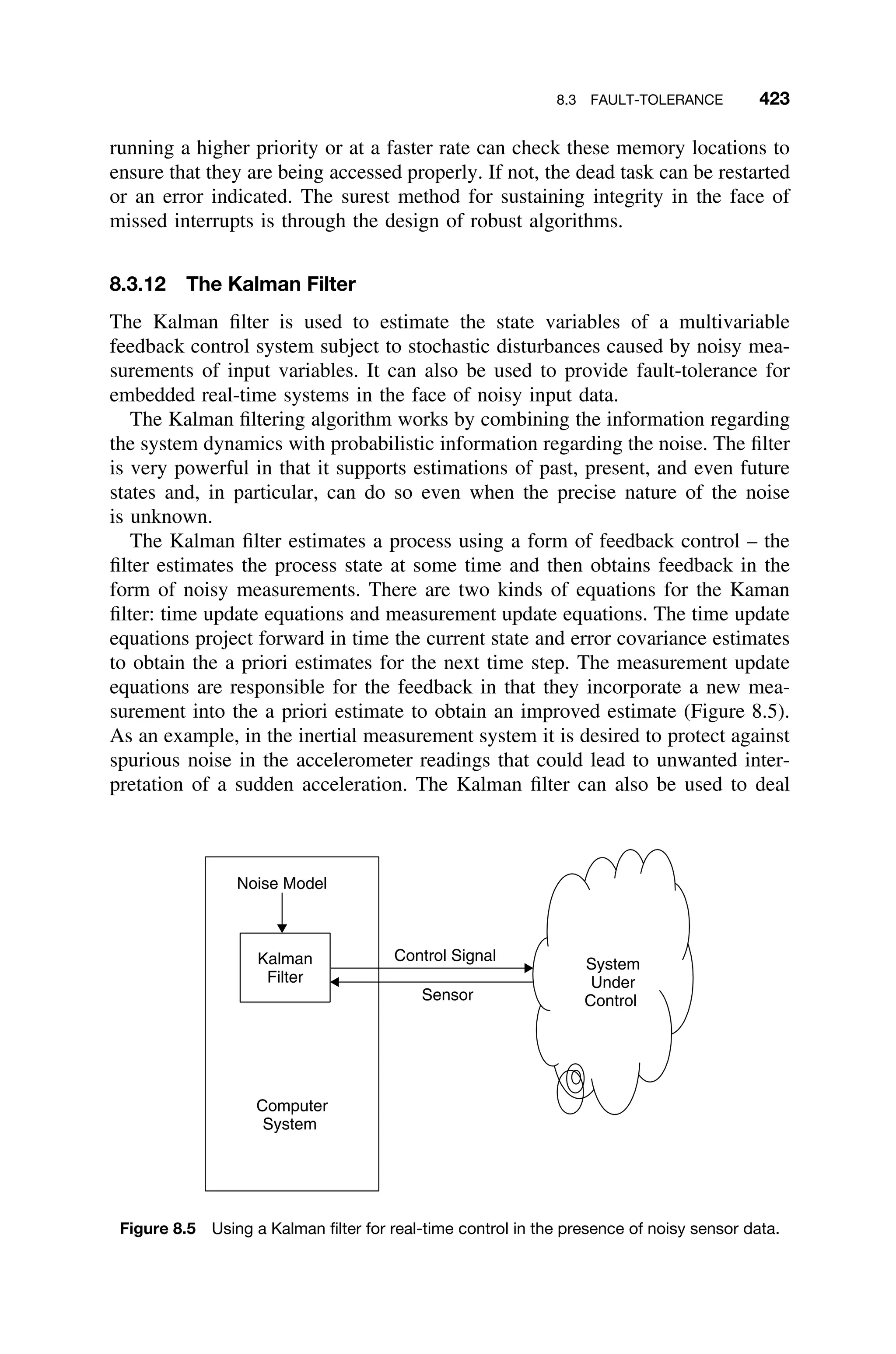
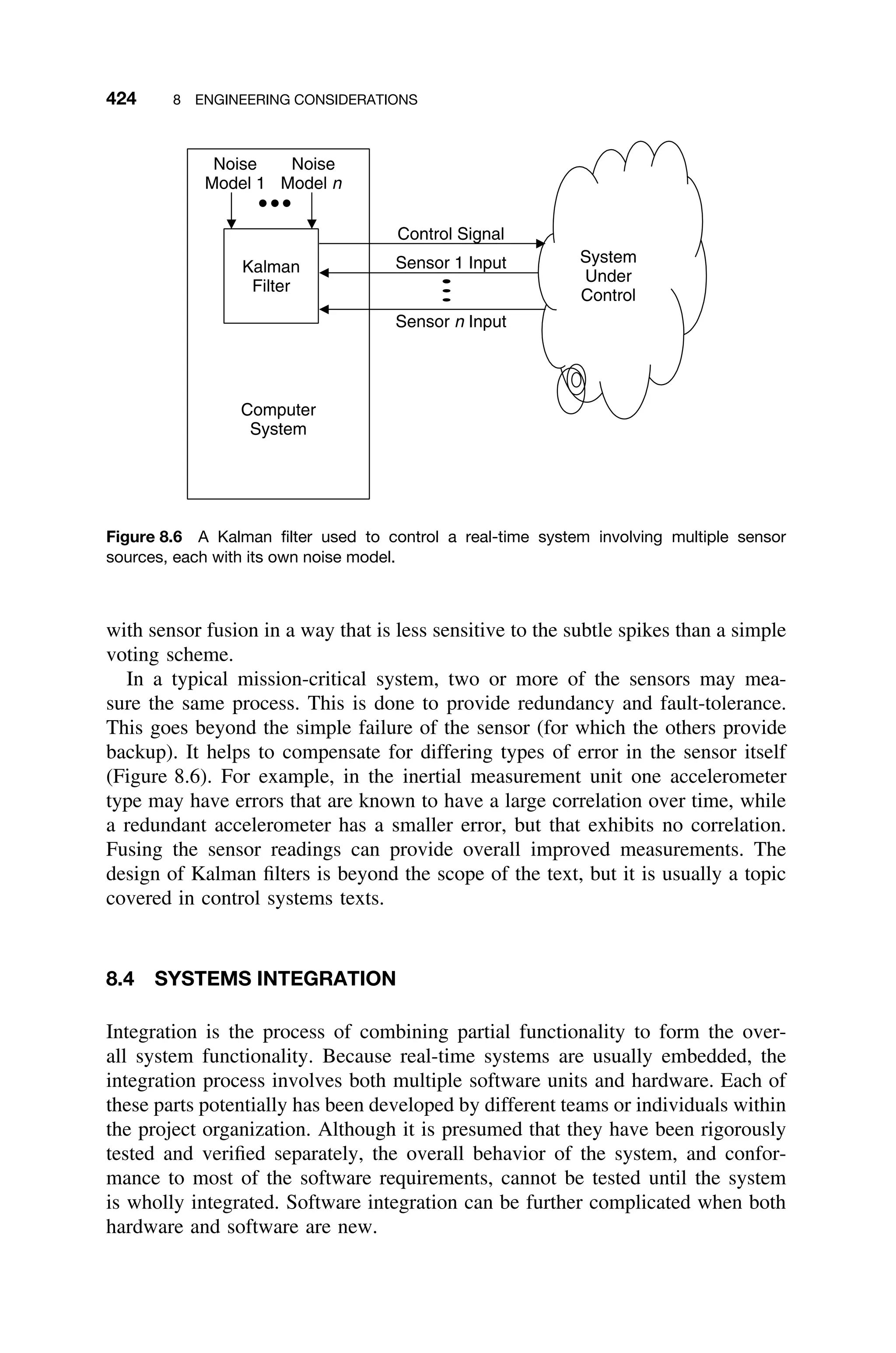
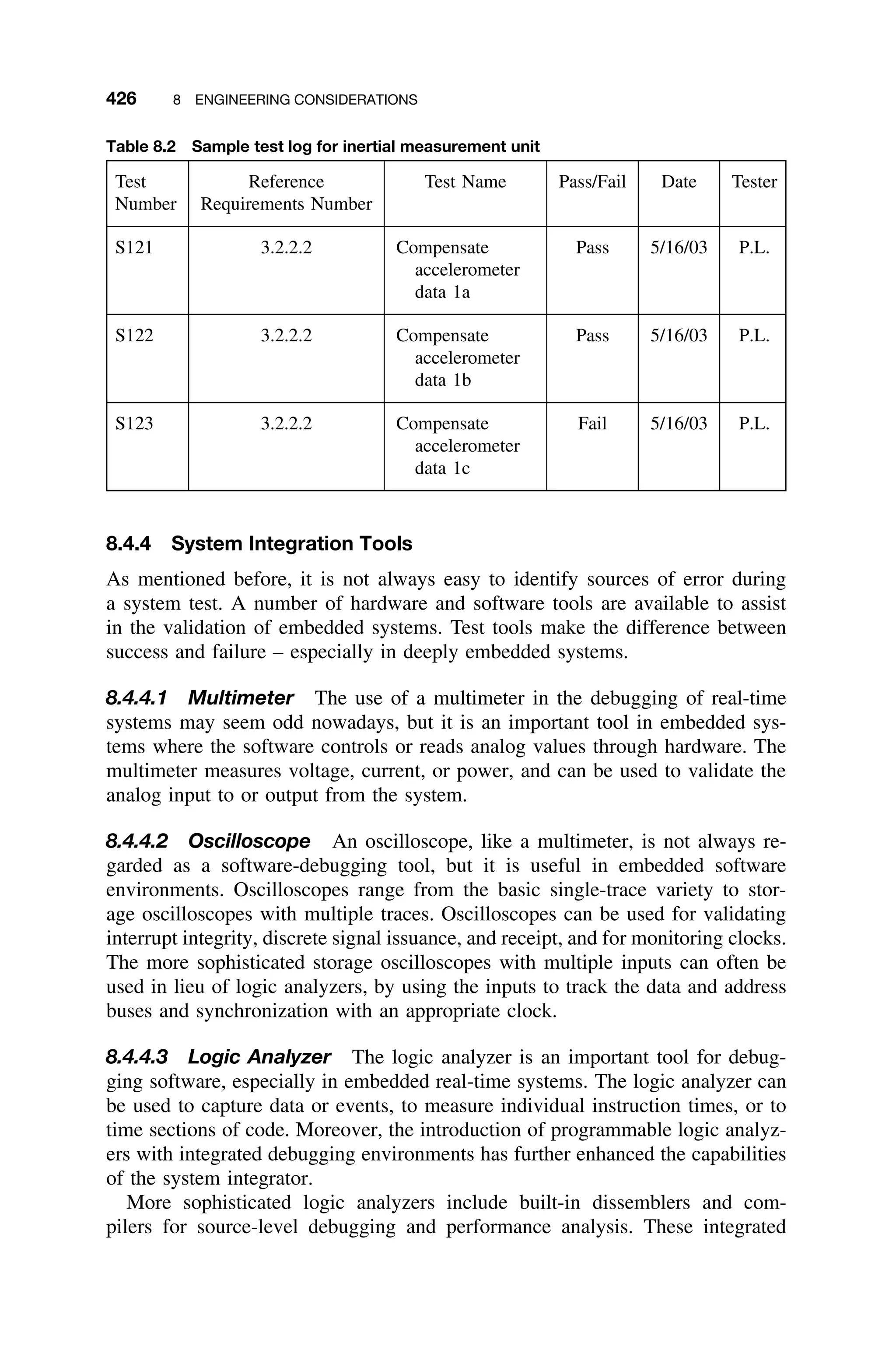
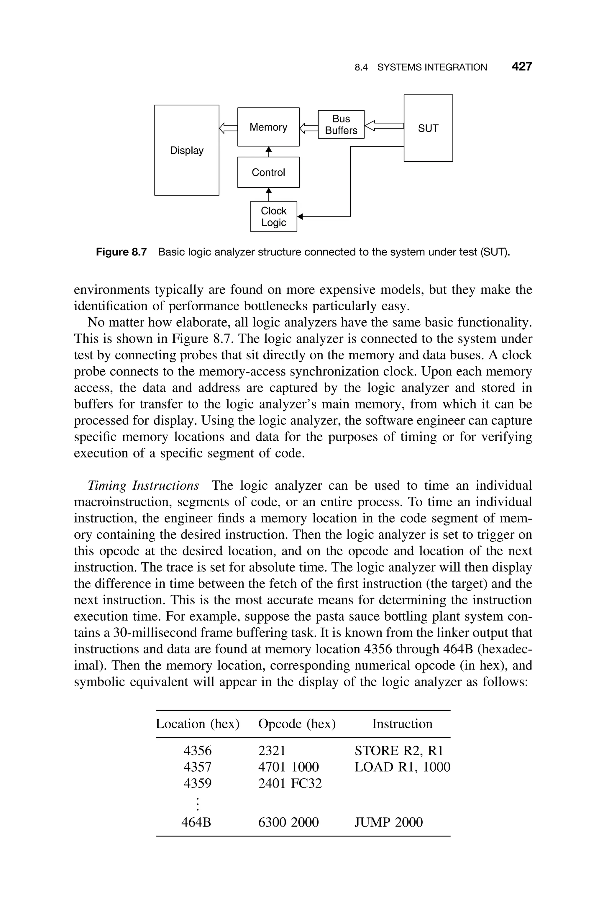
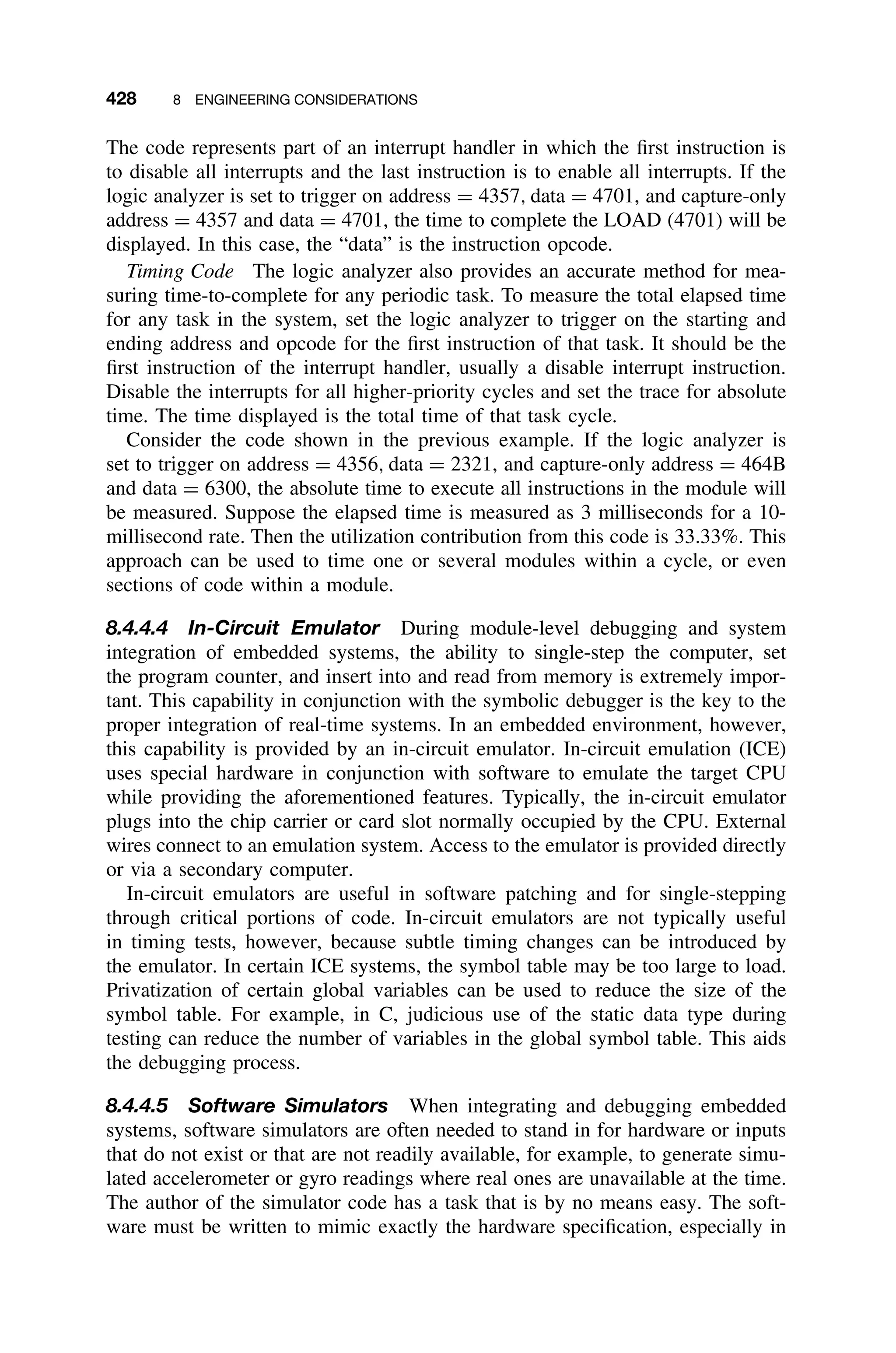
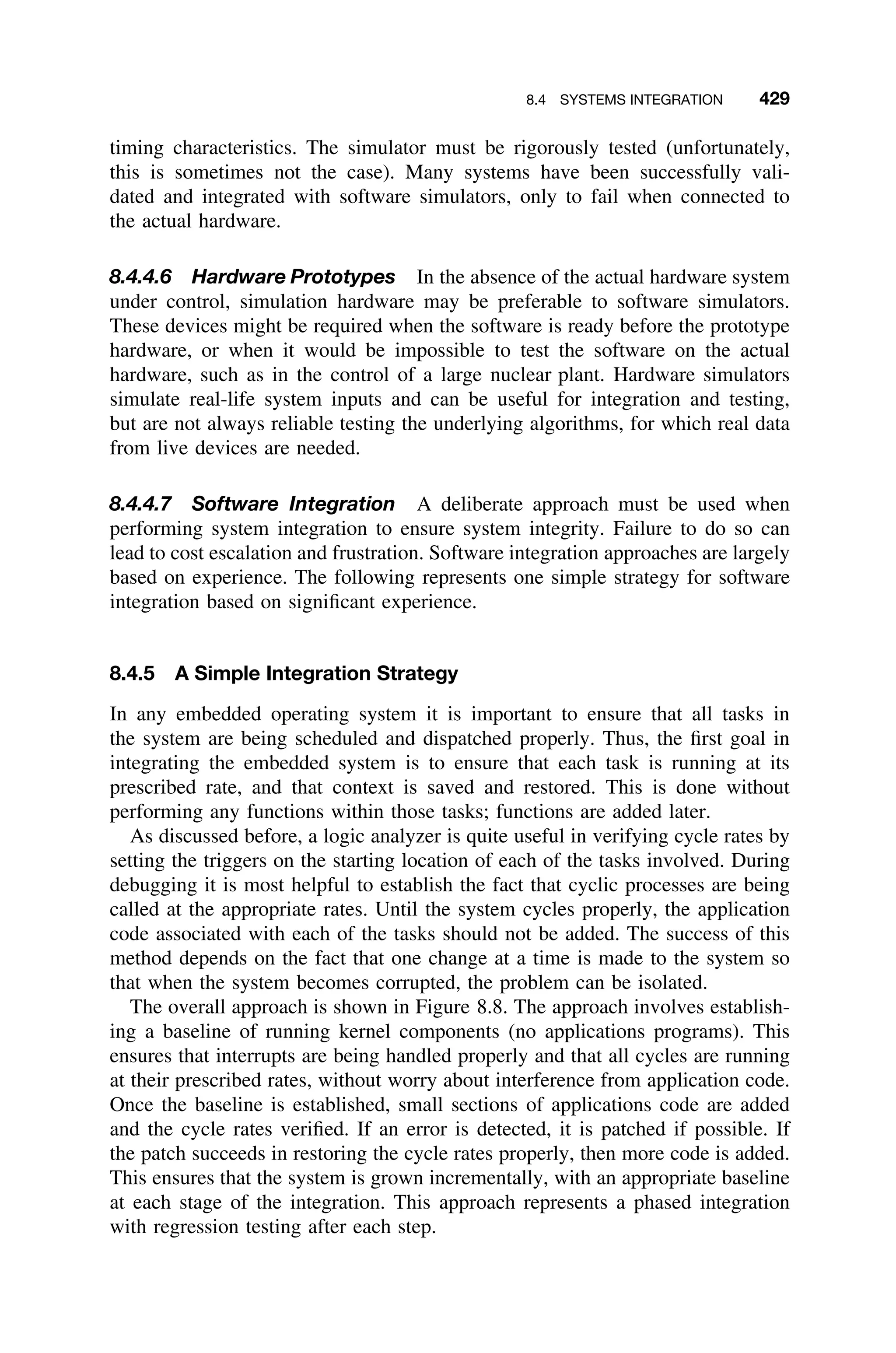
![430 8 ENGINEERING CONSIDERATIONS
Establish
Baseline
Add Code
Test
Error Patch
Figure 8.8 A simple integration strategy [Laplante03c].
8.4.6 Patching
The process of correcting errors in the code directly on the target machine is called
patching. Patching allows minor errors detected during the integration process
to be corrected directly on the target machine, without undergoing the tedious
process of correcting the source code and creating a new load module. It is also
useful in repairing software remotely, for example, in space-borne applications.
Patching requires an expert command of the opcodes for the target machine
unless a macroassembly-level patching facility is available. It also requires an
accurate memory map, which includes the contents of each address in memory,
and a method for inserting directly into memory. This capability is provided by
many commercial development environments and by in-circuit emulators.
Patching, which is analogous to placing jumper wires on prototype hardware,
typically requires only a minor change of memory contents. If the patch needed
fits into the memory space accorded to the code to be changed, then it is consid-
ered an in-line patch. In Figure 8.9, for example, a 1 was supposed to be added
to register 1 (R1) instead of a 0. This error can be changed easily by altering the
memory location containing the LOAD R1,0 instruction to LOAD R1,1.
If the patch requires more memory than is currently occupied by the code to be
replaced, it is considered an oversized patch. In this case a JUMP to some unused
portion of memory is required, followed by the patched code, followed by a return
JUMP to the next significant location. This technique is shown in Figure 8.10. The
loading of patches during system integration can often be automated. However,
a large number of patches and patches on top of others can become confusing. It
is imperative that a careful record be kept of all patches made, that the patches
eventually find their way back to the source code, and that a new system be
generated before validation testing begins. This is essential from a maintenance
standpoint. Final testing should never be performed on a patched system.](https://image.slidesharecdn.com/epdf-230618090952-bdcb6616/75/epdf-pub_real-time-systems-design-and-analysis-pdf-453-2048.jpg)
![8.4 SYSTEMS INTEGRATION 431
LOAD R1,0
ADD R1,R2
STORE R1,@×1
LOAD R1, 1
Figure 8.9 In-line patch.
JUMP
(added
code)
JUMP
Figure 8.10 An oversized patch [Laplante03c].
Patching of software written in object-oriented languages is very difficult
because of the lack of a straightforward mapping from the source code to the
object code. Symbolic debuggers are quite helpful in this case, but even so, in
this situation patching is risky at best.
8.4.7 The Probe Effect
The uncertainty principle, originally postulated by Werner Heisenberg in 1927,
states essentially that the precise position and momentum of a particle cannot
be known simultaneously. An analogy to the Heisenberg uncertainty principle
applies in software integration. While software systems do not explicitly deal
with electrons (except as ensemble behavior), uncertainty arises because the more
closely a system is examined, the more likely the examination process will affect
the system. This fact is especially true for embedded systems where test probes](https://image.slidesharecdn.com/epdf-230618090952-bdcb6616/75/epdf-pub_real-time-systems-design-and-analysis-pdf-454-2048.jpg)
![432 8 ENGINEERING CONSIDERATIONS
can affect timing. For example, an engineer is debugging the pasta sauce bottling
system and discovers that a certain deadline is not being met. Some debugging
code is added to print out a preliminary result to a file. But after adding the
debugging code, the problem goes away. Declaring success, the engineer removes
the debugging code and the problem reappears. In this case, it is clear that the
debugging code somehow changed the timing of the system.
The software version of the Heisenberg uncertainty principle should be taken
as a warning that testing methods often affect the systems that they test. When
this is the case, nonintrusive testing should be considered, for example, using
a logic analyzer. Furthermore, wherever there is an inverse correlation between
two variables affecting system, Heisenberg uncertainty is suggested.
8.4.8 Fault-Tolerant Design: A Case Study
It has already been noted that single-bit errors present significant problems to
control systems operating in space or in the presence of a nuclear event, such as
in the control system for the nuclear energy plant. As a detailed example of a
fault-tolerant design for such an environment, consider the inertial measurement
system for the space shuttle [Laplante93].
8.4.8.1 Problem Description In understanding the potential effects of sin-
gle-event upsets (SEU), recall that different devices have varying susceptibilities
to upset partly based on geometry, logic levels, and manufacturing process. These
susceptibilities are summarized in Table 8.3. Depending on its mission, envi-
ronment, technology used, and other factors, the expectation of error can be
quite low. But the point here really is to illustrate a holistic approach to fault-
tolerant design.
8.4.8.2 Hardware Support Certain parts manufacturers design and test crit-
ical components for radiation hardness. In many cases, parts are preirradiated with
low-level radiation to liberate any radioactive impurities in the packaging mate-
rial that could have become offending particles or created latch-ups. This process
may lower the part’s SEU potential. However, this treatment diminishes the part’s
low-level radiation longevity. In addition to minimizing SEU rates through opti-
mum part selection, error detection and correction should be used. For the space
shuttle internal measurement unit (IMU) application the AMD2960 was selected
to protect the 8K RAM and 4K of EEPROM used for crucial data.
8.4.8.3 Software Fault-Tolerant Various measures can be taken during
system start up, foreground processing, and background processing to enhance
fault-tolerance. The software for the space shuttle IMU was particularly aggres-
sive in this regard.
Initialization During initialization it is necessary to perform as many system-
level and device-level checks as possible. There is usually plenty of time to](https://image.slidesharecdn.com/epdf-230618090952-bdcb6616/75/epdf-pub_real-time-systems-design-and-analysis-pdf-455-2048.jpg)
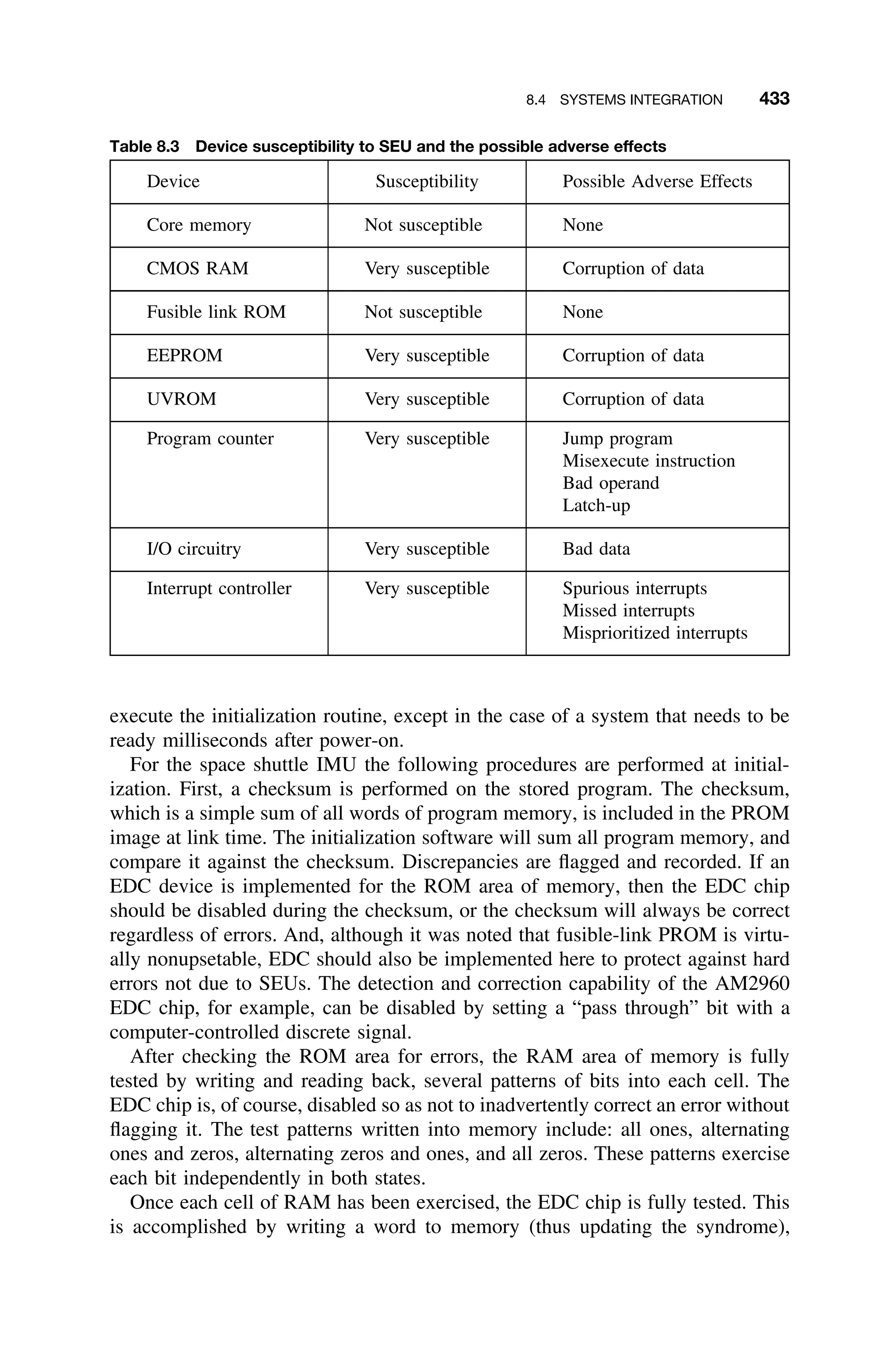
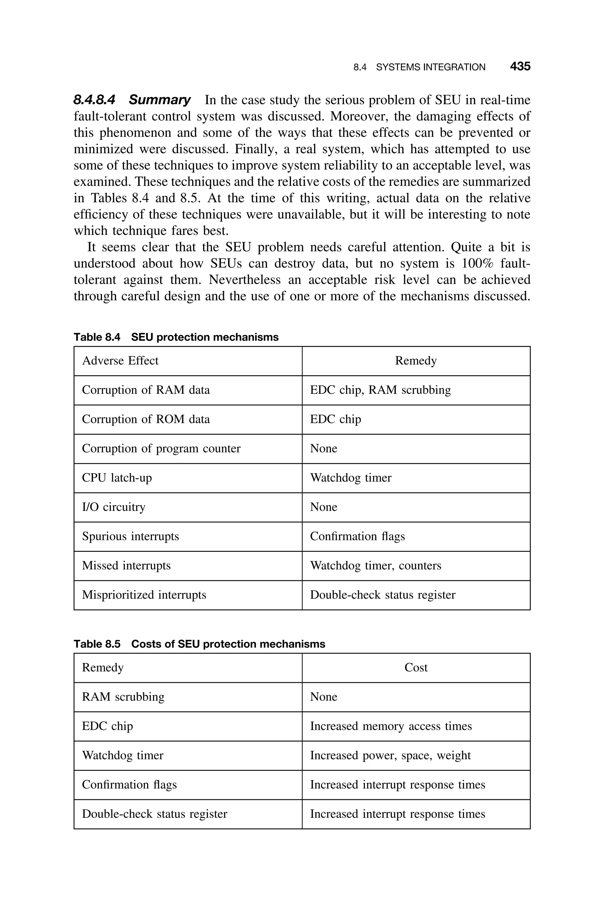
![436 8 ENGINEERING CONSIDERATIONS
8.5 REFACTORING REAL-TIME CODE
A code smell is a popular term that refers to an indicator of poor design or coding
[Fowler00]. More specifically, the term relates to visible signs that suggest the
need for refactoring. Refactoring refers to a behavior preserving code transfor-
mation enacted to improve some feature of the software, which is evidenced by
the code smell.
The notion of refactoring, however, is ordinarily associated with object-oriented
code [Fowler00]. On the other hand, code smells are found in both object-oriented
and procedurally oriented code in real-time systems, especially legacy systems.
In this section a brief discussion of some of the more common code smells and
their refactorings are given. Applying these refactorings appropriately can help to
enhance desirable properties of the software while removing the undesirable ones.
8.5.1 Conditional Logic
There are several reasons why excessive switch, if-then, and case state-
ments are an indicator of a bad design in real-time systems. First, they breed
code duplication. Moreover, the code generated for a case statement can be quite
convoluted, for example, a jump through a register, offset by a table value. This
mechanism can be time-consuming. Furthermore, nested conditional logic can be
difficult to test, especially if it is nested due to the large number of logic paths
through the code. Finally, the differences between best- and worst-case execution
times can be significant, leading to highly pessimistic utilization figures.
Conditional logic needs to be refactored, but there is no silver bullet here. In
dealing with performance issues, often trade-offs can be made by exchanging one
type of conditional logic for another. For example, in some compilers, the case
statement is efficient only if more than three cases are to be compared, otherwise,
nested if statements should be used. Reducing the switch logic (and hence, the
number of conditionals) can also be accomplished through application of logical
identities, and in the most complex cases, through traditional logic minimization
techniques such as Karnaugh mapping and the Quine-McCluskey procedure.
8.5.2 Data Clumps
Several data items found together in lots of places are known as data clumps. In
the procedural sense data clumps can arise, for example, in C from too much con-
figuration information in #include files. Stewart calls this problem “#include
globals.h” and notes that this situation is unhealthy because it leads to increased
development and maintenance time and introduces circular dependencies that
make reuse difficult. He suggests that to refactor, each module be defined by
two files “.h” and “.c,” with the former containing only that information that
is to be exported by the module and “.c” file containing everything that is not
exported [Stewart99].
A second manifestation of the data clump smell has to do with excessive use of
#define statements that propagate through the code. Suppose these #defines](https://image.slidesharecdn.com/epdf-230618090952-bdcb6616/75/epdf-pub_real-time-systems-design-and-analysis-pdf-459-2048.jpg)
![8.5 REFACTORING REAL-TIME CODE 437
are expanded in 20 places in the code. If, during debugging, it is desired to place
a patch over one of the #defines, it must be done in 20 places. To refactor,
place the quantity in a global variable that can be changed in one place only
during debugging [Stewart99].
8.5.3 Delays as Loops
Another code smell involves timing delays implemented as while loops with
zero or more instructions [Stewart99]. These delays rely on the overhead cost
of the loop construct plus the execution time of the body to achieve a delay.
The problem is that if the underlying architecture changes or characteristics of
instruction execution (e.g., memory access time) changes, then the delay time
is inadvertently altered. To refactor use a mechanism based on a timer facility
provided by the operating system that is not itself based on individual instruction
execution times.
8.5.4 Dubious Constraints
This code smell is particularly insidious in real-time systems where response-time
constraints have questionable or no attributable source. In some cases, systems
have deadlines that are imposed on them that are based on nothing less than
guessing or on some forgotten and since eliminated requirement. The problem in
these cases is that undue constraints may be placed on the systems. For example,
suppose the response time for an interrupt is 30 ms, but no one knows why.
Similarly, more than one reason given for the constraints in comments or docu-
mentation indicates a traceability conflict, which hints at other problems. This is
a primary lesson in using real-time systems design to understand the basis and
nature of the timing constraints, so that they can be relaxed if necessary.
In any case, to remove the code smell, some detective work is needed to
discover the true reason for the constraint. If it cannot be determined, then the
constraint could be relaxed and the system redesigned accordingly.
8.5.5 Duplicated Code
Obviously, duplicated code refers to the same or similar code found in more
than one place. This code has an unhealthy impact on maintainability (the same
change has to be propagated to each copy), and it also adversely affects memory
utilization.
It is obvious that the purpose of refactoring is to assign the code to a single
common code unit via better application of information hiding. While it is too
easy to mock the designers of systems that contain duplicated code, it is possible
that the situation arose out of a real need at the time. For example, duplicated
code may have been due to legacy concerns for performance where the cost of the
procedure call added too much overhead in a critical instance. Alternatively, in
languages that were not reentrant, such as early versions of Fortran, duplicated](https://image.slidesharecdn.com/epdf-230618090952-bdcb6616/75/epdf-pub_real-time-systems-design-and-analysis-pdf-460-2048.jpg)
![438 8 ENGINEERING CONSIDERATIONS
code was a common means for providing utilities to each cycle in the real-
time system.
8.5.6 Generalizations Based on a Single Architecture
Stewart suggests that writing software for a specific architecture, but with the
intent to support easy porting to other architectures later, can lead to overgen-
eralizing items that are similar across architectures, while not generalizing some
items that are different. He suggests developing the code simultaneously on mul-
tiple architectures and then generalizing only those parts that are different. He
suggests choosing three or four architectures that are very different in order to
obtain the best generalization [Stewart99]. Presumably, such an approach suggests
the appropriate refactoring.
8.5.7 Large Procedures
Fowler describes two code smells, long method and large class, which are
self-evident. In the procedural sense, the analogy is a large procedure. Large pro-
cedures are anathema to the divide-and-conquer principle of software engineering
and need to be refactored by repartitioning the code appropriately.
8.5.8 Lazy Procedure
A lazy method is one that does not do enough to justify its existence. The
procedural analogy to the lazy class/method code smells is the lazy procedure.
In a real-time sense, a procedure that does too little to pay for the overhead of
calling the procedure needs to be eliminated by removing its code to the calling
procedure(s), or redefining the procedure to do more.
8.5.9 Long Parameter List
Long parameter lists are an unwanted remnant of the practice of using parameter
lists to avoid the use of global variables. While well-defined interfaces are clearly
desirable, long parameter lists can cause problems in real-time systems if inter-
rupts are disabled during parameter passing. In this case, overly long interrupt
latencies and possible missed deadlines are possible. The “long parameter list”
code smell can be refactored by passing a pointer to one or more data structures
that contain aggregated parameters, or by using global variables.
8.5.10 Message-Passing Overload
Stewart describes the excessive use of message passing for synchronization as
another unwanted practice. He notes that this practice can lead to unpredictabil-
ity (because of the synchronization necessary), the potential for deadlock, and
the overhead involved. He suggests that the refactoring is to use state-based
communication via shared memory with structured communication [Stewart99].](https://image.slidesharecdn.com/epdf-230618090952-bdcb6616/75/epdf-pub_real-time-systems-design-and-analysis-pdf-461-2048.jpg)
![8.5 REFACTORING REAL-TIME CODE 439
8.5.11 Self-Modifying Code
One method that can be used to save space in the code area of memory is self-
modifying code. This method takes advantage of the fact that the opcodes of
certain instructions may differ by only one bit. For example, by flipping a bit
in a JUMP instruction, an ADD instruction is created. Although this type of
programming usually arises from coincidence, stories exist about programmers
who could write such code effortlessly. In fact, in some settings, it was considered
a sign of cleverness to include some self-modifying code. The most important
disadvantage of such coding is that it destroys determinism.
Unfortunately, many processors include on-chip caches that can obviate self-
modifying code. In these cases the cache does not update the code and executes
the unmodified code. Additionally, the effect of modifying code within the cache
causes performance degradation. In any case, this type of programming should
never be done, but was not uncommon in older systems.
8.5.12 Speculative Generality
Speculative generality relates to hooks and special cases that are built into the
code to handle things that are not required (but might be needed someday). Real-
time systems are no place to build in hooks for “what-if” code. Hooks lead to
testing anomalies and possible unreachable code. Therefore, the refactoring is to
remove hooks and special cases that are not immediately needed.
8.5.13 Telltale Comments
The telltale comment problem appears in real-time and non-real-time systems.
Comments that are excessive, or that tend to explicate the code beyond a rea-
sonable level are often indicators of some serious problem. Comments such as:
ž “Do not remove this code.”
ž “If you remove this statement the code doesn’t work, I don’t know why.”
ž “Please see me for an explanation of this code . . . .”
are not uncommon. Humor in comment statements can sometimes be a glib way
to mask the fact that writer does not know what he or she is doing. For example,
“if you understand this code, could you please explain it to me?” Clearly these
kinds of statements indicate that there are underlying timing errors. In the case of
tell-tale comments, the refactoring involves rewriting the code so that an overly
long explicating comment is not necessary.
8.5.14 Unnecessary Use of Interrupts
Stewart also suggests that indiscriminate use of interrupts is a bad code smell
[Stewart99]. Interrupts can lead to deadlock, priority inversion, and the inability to](https://image.slidesharecdn.com/epdf-230618090952-bdcb6616/75/epdf-pub_real-time-systems-design-and-analysis-pdf-462-2048.jpg)
![440 8 ENGINEERING CONSIDERATIONS
make performance guarantees. Interrupt-based systems should be avoided, though
as has been noted, this is possible only in the simplest of systems where real-time
multitasking can be achieved with coroutines and cyclic executives implemented
without interrupts. When interrupts are required to meet performance constraints,
rate-monotonic or earliest deadline first scheduling should be used.
8.6 COST ESTIMATION USING COCOMO
Cost estimation is an important component of engineering real-time software
systems. One of the most widely used software modeling tools is Boehm’s
COCOMO model, first introduced in 1981 [Boehm81]. COCOMO is an acronym
for constructive cost model. That is, it is a predictive model. There are three ver-
sions of the original COCOMO: basic, intermediate and detailed, and the recently
released COCOMO II model.
8.6.1 Basic COCOMO
The basic COCOMO model is based on thousands of lines of deliverable source
instructions. In short, for a given piece of software, the time, T , to complete is a
function of L, the number of lines of delivered source instructions (KDSI), and
two additional parameters, a and b, which will be explained shortly. This is the
effort equation for the basic COCOMO model:
T = aLb
(8.13)
Dividing T by a known productivity factor, in KLOC per person month, yields
the number of person months estimated to complete the project.
The parameters a and b are a function of the type of software system to
be constructed. For example, if the system is organic, that is, one that is not
heavily embedded in the hardware, then the following parameters are used: a =
3.2, b = 1.05. If the system is semidetached, that is, partially embedded, then
these parameters are used: a = 3.0, b = 1.12. Finally, if the system is embedded,
that is closely tied to the underlying hardware like the inertial measurement
system, then the following parameters are used a = 2.8, b = 1.20. Note that the
exponent for the embedded system is the highest, leading to the longest time to
complete for an equivalent number of delivered source instructions.
Recall that for the inertial measurement system, using feature points, 37.6 thou-
sand lines of C code were estimated. Hence, an effort-level estimate is obtained
using COCOMO of:
T = 2.8 · (37.6K)1.2
= 169K
Suppose, then, it is known that an efficient software engineer using computer-
aided software engineering (CASE) and other tools can generate 2000 lines of
code per month. Then superficially, at least, it might be estimated that the project](https://image.slidesharecdn.com/epdf-230618090952-bdcb6616/75/epdf-pub_real-time-systems-design-and-analysis-pdf-463-2048.jpg)
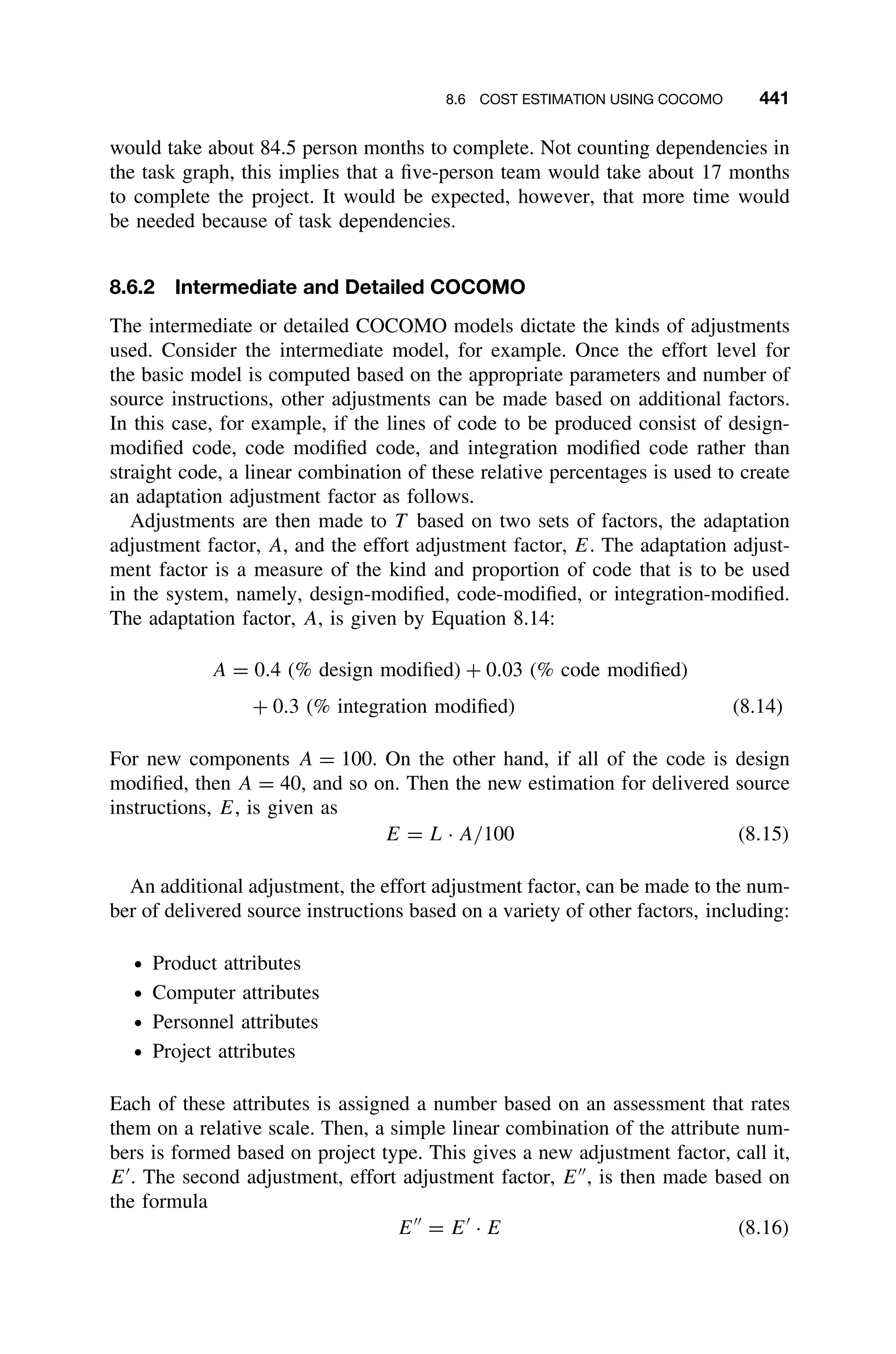

![BIBLIOGRAPHY
[Allard91] Allard, J. R., and Hawkinson, L. B. “Real-Time Programming in Common LISP.”
Communications of the ACM, Volume 35, Number 9, September 1991, pp. 64–69.
[Allworth87] Allworth, S. T., and Zobel, R. N. Introduction to Real-Time Software Design, 2nd
Edition. Springer-Verlag, New York, 1987.
[Amdahl67] Amdahl, G. M. “Velocity of the Single-Processor Approach to Large Scale Com-
puting Capabilities.” Proceedings of AFIPS, Volume 30. Atlantic City, NJ, April 18–20,
AFIPS Press, Reston: VA, 1967, pp. 483–485.
[Avrunin98] Avrunin, G., Corbett, J., and Dillon, L. “Analyzing Partially-Implemented Real-
Time Systems.” IEEE Transactions on Software Engineering, Volume 24, Number 8, August
1998, pp. 602–614.
[Baker90] Baker, T. P. “A Stacked-Based Resource Allocation Policy for Real-Time Pro-
cesses.” Proceedings of the 11th Real-Time Systems Symposium. Lake Buena Vista, FL,
December 1990, pp. 191–200.
[Ball00] Ball, S. Embedded Microprocessor Systems. Newnes, Boston: MA, 2000.
[Barr99] Barr, M. Programming Embedded Systems in C and C++. O’Reilly and Associates,
Sebastopol, CA, 1999.
[Bartee91] Bartee, T. C. Computer Architecture and Logic Design. McGraw-Hill, New York,
1991.
[Baruah90] Baruah, S. K., Mok, A. K., and Rosier, L. E. “Preemptively Scheduling Hard Real-
Time Sporadic Tasks on One Processor.” Proceedings of the 11th Real-Time Systems Sym-
posium. Lake Buena Vista, FL, December 1990, pp. 182–190.
[Beck99] Beck, K. Extreme Programming Explained: Embrace Change. Addison-Wesley, New
York, 1999.
[Berger02] Berger, A. Embedded Systems Design: An Introduction to Processes, Tools, Tech-
niques. CMP Books, Lawrence: KS, 2002.
[Bergman93] Bergman, G. D. Electronic Architectures for Digital Processing: Software/Hard-
ware Balance in Real-Time Systems. Prentice Hall, Englewood Cliffs, NJ, 1993.
[Blackman75] Blackman, M., The Design of Real-Time Applications. John Wiley Sons, New
York, 1975.
[Blum92] Blum, B. I. Software Engineering: A Holistic View. Oxford University Press, New
York, 1992.
[Bodilsen94] Bodilsen, S. “Scheduling Theory and Ada 9X.” Embedded Systems Programming.
December 1994, December pp. 32–52.
[Boehm81] Boehm, B. Software Engineering Economics. Prentice Hall, Englewood Cliffs, NJ,
1981.
Real-Time Systems Design and Analysis, By Phillip A. Laplante
ISBN 0-471-22855-9 2004 Institute of Electrical and Electronics Engineers
475](https://image.slidesharecdn.com/epdf-230618090952-bdcb6616/75/epdf-pub_real-time-systems-design-and-analysis-pdf-498-2048.jpg)
![476 BIBLIOGRAPHY
[Bollella00a] Bollella, G., and Gosling, J. “The Real-Time Specification for Java.” IEEE Com-
puter, June 2000, Volume 33, Number 6, pp. 47–54.
[Bollella00b] Bollella, G., Brosgol, B., Furr, S., Hardin, D., Dibble, P., Gosling, J., and Turn-
bull, M. The Real-Time Specification for Java. Addison-Wesley, Boston, MA, 2000.
[Booch99] Booch, G., Jacobson, I., and Rumbaugh, J. The Unified Modeling Language User’s
Guide. Addison-Wesley, Boston, MA, 1999.
[Booch91] Booch, G. Object-Oriented Design with Applications, Benjamin Cummings, New
York, 1991.
[Boussinot91] Boussinot, F., and DeSimmi, R. “The ESTEREL Language.” Proceedings of the
IEEE, Volume 79, Number 9, September 1991, pp. 1293–1304.
[Bowen95] Bowen, J. P. and Hinchey, M. G. “Ten Commandments of Formal Methods.” IEEE
Computer, Volume 28, Number 4, April 1995, pp. 56–63.
[Brooks95] Brooks, F. The Mythical Man-Month, 2nd
Edition. Addison-Wesley, New York,
1995.
[Bucci95] Bucci, G., Campanai, M., and Nesi, P. “Tools for Specifying Real-Time Systems.”
Real-Time Systems: The International Journal of Time Critical Systems, Volume 8, Number
2/3, March/April 1995, pp. 117–172.
[Burns90] Burns, A. and Wellings, A. Real-time Systems and Their Programming Languages.
Addison-Wesley, New York, 1990.
[Buttazzo00] Buttazzo, G. Hard Real-Time Computing Systems: Predictable Scheduling Algo-
rithms and Applications. Kluwer Academic Publishers, Norwell, MA, 2000.
[Calvez93] Calvez, J. P., Wyche, A., and Edmundson, C. (Translators). Embedded Real-Time
Systems/a Specification and Design Methodology. John Wiley Sons, New York, 1993.
[Campbell88] Campbell, J. C Programmer’s Guide to Serial Communications. Howard Sams
Co., Indianapolis, IN, 1988.
[Cardelli96] Cardelli, L. “Bad Engineering Properties of Object-Oriented Languages.” ACM
Computing Surveys, Volume 28A, Number 4, December 1996, pp. 150–158.
[Chiodo94] Chiodo, M., Giusto, P., Jurecska, A., Marelli, M., Hsieh, H., Sangiovanni-
Vincentelli, A., and Lavagno, L. “Hardware-Software Codesign of Embedded Systems.”
IEEE Micro, Volume 14, Number 4, August 1994, pp. 26–36.
[Clark91] Clark, E. M. Jr., Long, D. E., and McMillen, K. “A Language for Computational
Specification and Verification of Finite State Hardware Controllers.” Proceedings of the
IEEE, Volume 79, Number 9, September 1991, pp. 1283–1292.
[Cnet00] CNet, “10 Great Bugs of History.” http://coverage.cnet.com/content/features/DLife/
Bugs/SS05i.html, accessed 9/13/2000.
[Cottet02] Cottet, F., Delacroix, J., Kaiser, C., and Mammeri, Z. Scheduling in Real Time Sys-
tems. John Wiley Sons, Chichester England, 2002.
[Craigen95] Craigen, D., Gerhart, S., and Ralston, T. “Formal Methods Reality Check: Indus-
trial Usage.” IEEE Transactions on Software Engineering, Volume 21, Number 2, February
1995, pp. 90–98.
[Crenshaw00] Crenshaw, J. Math Toolkit for Real-Time Programming. CMP Books, Lawrence,
KS, 2000.
[Daigle92] Daigle, J. N. Queuing Theory for Telecommunications. Addison-Wesley, New York,
1992.
[Davari93] Davari, S., Leibfried, T. F. Jr., Natarajan, S., Pruett, D., Sha, L., and Zhao, W.
“Real-Time Issues in the Design of the Data Management System for the Space Station
Freedom.” Proceedings of the First Real-Time Applications Workshop, July 1993, IEEE CS
Press, New York, pp. 161–165.
[Davis73] Davis, M. Computability and Unsolvability. Dover Publishing Co., New York, 1973.
[de la Puente00] de la Puente, J. “Real-Time Object-Oriented Design and Formal Methods.”
The International Journal of Time-Critical Computing Systems, Volume 18, Number 1 2000,
pp. 79–83.](https://image.slidesharecdn.com/epdf-230618090952-bdcb6616/75/epdf-pub_real-time-systems-design-and-analysis-pdf-499-2048.jpg)
![BIBLIOGRAPHY 477
[DeMarco78] DeMarco, T. Structured Analysis and System Specification. Prentice Hall, Engle-
wood Cliffs, NJ, 1978.
[DeMillo79] DeMillo, R. A., Lipton, R. J., and Perlis, A. “Social Processes and Proofs of The-
orems and Programs.” Communications of the ACM, Volume 22, Number 5, May 1979,
pp. 271–280.
[Desmonde64] Desmonde, W. H. Real-Time Data Processing Systems: Introductory Concepts.
Prentice Hall, Englewood Cliffs, NJ, 1964.
[Dibble02] Dibble, P. Real-Time JAVA Platform Programming. Sun Microsystems, Inc., Palo
Alto, CA, 2002.
[Dijkstra68a] Dijkstra, E. W. “Goto Statement Considered Harmful.” Communications of the
ACM, Volume 11, Number 3, March 1968, pp. 147–148.
[Dijkstra68b] Dijkstra, E. W. “Solution of a Problem in Concurrent Programming Control.”
Communications of the ACM, Volume 11, Number 3, March 1968, page 569.
[Dijkstra65] Dijkstra, E. W. “Cooperating Sequential Processes.” Technical Report EWD-123,
Technological University, Eindhoven, Netherlands, 1965.
[DOD-STD88] DOD-STD-2167A. Military Standard Defense System Software Development.
U.S. Department of Defense, Washington: DC, 1988.
[Dougherty95a] Dougherty, E. R., and Laplante, P. A. Introduction to Real-Time Image Pro-
cessing, SPIE Press/IEEE Press, Bellingham, WA, January 1995.
[Douglass03] Douglass, B. P. Real-Time Design Patterns: Robust Scalable Architecture for
Real-Time Systems. Addison-Wesley, Boston, MA, 2003.
[Douglass99] Douglass, B. P., Doing Hard Time – Developing Real-Time Systems with UML,
Objects, Frameworks, and Patterns. Addison-Wesley Longman, Reading, MA, 1999.
[Douglass99] Douglass, B. P., Real-Time UML, Second Edition, Developing Efficient Objects
for Embedded Systems. Addison-Wesley Longman, Reading, MA, 1999.
[Edwards93] Edwards, K. Real-Time Structured Methods: Systems Analysis, John Wiley
Sons, New York, 1993.
[Electronic Industry98a] Electronic Industry Association, EIA 709.1-1998, Control Network
Protocol Specification. 1998, Arlington, VA.
[Electronic Industry98b] Electronic Industry Association, EIA 709.3-1998, Free Topology
Twisted Pair Channel Specification. 1998, Arlington, VA.
[Ellis94] Ellis, J. R. Objectifying Real-Time Systems. Prentice Hall, Englewood Cliffs, NJ, 1994.
[Fenton96] Fenton, N. Software Metrics: A Rigorous Approach. Chapman Hall, London,
1996.
[Ferrintino77] Ferrintino, A. B., and Mills, H. D. “State Machines and Their Semantics in
Software Engineering.” Proceedings of the IEEE COMPSAC Conference, 1977, pp. 242–251.
[Fetzer88] Fetzer, J. H. “Program Verification: The Very Idea.” Communications of the ACM,
Volume 31, Number 9, September 1988, pp. 1048–1062.
[Flynn66] Flynn, M. J. “Very High-Speed Computing Systems.” IEEE Transactions on Com-
puting. Volume 54, Number 12, December 1966, pp. 1901–1909.
[Forestier89] Forestier, J. P., Forarino, C., and Franci-Zannettacci, P. “Ada++: A Class and
Inheritance Extension for Ada.” Proceedings of Ada-Europe International Conference,
Madrid. Ada Companion Series. Cambridge University Press, Cambridge, June 1989.
[Foster81] Foster, C. Real Time Programming- Neglected Topics. Addison-Wesley, Reading,
MA, 1981.
[Fowler00] Fowler, M. Refactoring. Addison-Wesley, New York, 2000.
[Frakes96] Frakes, W. B., and Fox, C. J. “Quality Improvement Using a Software Reuse Fail-
ure Modes Model.” IEEE Transactions on Software Engineering, Volume 22, Number 4,
April 1996, pp. 274–279.
[Freedman77] Freedman, A. L., and Lees, R. A. Real-Time Computer Systems. Crane, Russak
Co., New York, 1977.](https://image.slidesharecdn.com/epdf-230618090952-bdcb6616/75/epdf-pub_real-time-systems-design-and-analysis-pdf-500-2048.jpg)
![478 BIBLIOGRAPHY
[Furht91] Furht, B., Grostick, D., Gluch, D., Rabbat, G., Parker, J., and McRoberts, M. Real-
Time Unix Systems Design and Application Guide. Kluwer Academic Publishers, Boston,
MA, 1991.
[Gamma94] Gamma, E., Helm, R., Johnson, R., and Vlissides, J. Design Patterns: Elements
of Reusable Object-Oriented Software. Addison-Wesley, New York, 1994.
[Gane79] Gane, C., and Saron, T., Structured Systems Analysis, Prentice Hall, Englewood
Cliffs, NJ, 1979.
[Garrett94] Garrett, P. H. Advanced Instrumentation and Computer I/O Design: Real-Time Sys-
tem Computer Interface Engineering. IEEE Press, Piscataway, NJ, 1994.
[Garver94] Garver, R. “How to Implement ISO 9000.” T D. September 1994, pp 36–42.
[Ghezzi91] Ghezzi, C., Jazayeri, M., and Mandriolo, D. Fundamentals of Software Engineer-
ing. Prentice Hall, Englewood Cliffs, NJ, 1991.
[Gilreath03] Gilreath, W., and Laplante, P. Computer Architecture: A Minimalist Perspective.
Kluwer Academic Publishers, Norwell, MA, 2003.
[Gomaa00] Gomaa, H. Designing Concurrent, Distributed and Real-Time Applications with
UML. Addison-Wesley, Boston, MA, 2000.
[Gomaa93] Gomaa, H. Software Designing Methods for Concurrent and Real-Time Systems.
Addison-Wesley, Reading, MA, 1993.
[Goodenough88] Goodenough, J. B., and Sha, L. “The Priority Ceiling Protocol: A Method for
Minimizing the Blocking of High-Priority Ada Tasks.” Technical Report CMU/SEI-88-SR-4.
Carnegie-Mellon University: Software Engineering Institute, Pittsburgh, PA, 1988.
[Gopinath93] Gopinath, P., Bihri, T., and Gupta, R. “Compiler Support for Object-Oriented
Real-Time Software.” IEEE Software, September 1993, pp. 42–49.
[Grehan98] Grehan, R., Moote, R., and Cyliax, I. Real-Time Programming: A Guide to 32-bit
Embedded Development, Chapter 9. Addison-Wesley, New York, 1998.
[Gustafson88] Gustafson, J. “Reevaluating Amdahl’s Law.” Communications of the ACM, Vol-
ume 31, Number 5, May 1988, pp. 532–533.
[Habermann69] Habermann, A. N. “Prevention of System Deadlocks.” Communications of the
ACM, Volume 12, Number 7, July 1969, pp. 171–176.
[Halang94] Halang, W. A., and Stoyenko, A. Real Time Computing. NATO ASI Series. Springer-
Verlag, Berlin, 1994.
[Halang91] Halang, W. A., and Stoyenko, A. Constructing Predictable Real-Time Systems.
Kleuwer Academic Publishers, Boston, MA, 1991.
[Halstead77] Halstead, M. H. Elements of Software Science. North-Holland, Amsterdam, 1977.
[Harbison91] Harbison, S. P., and Steele, G. L. Jr. C: A Reference Manual. Prentice Hall,
Englewood Cliffs, NJ, 1991.
[Harel90] Harel, D., Lanchover, H., Naamad, A., Pnueli, A., Politi, M., Sherman, R., and Trau-
ring, A. “STATEMATE: A Working Environment for the Development of Complex Reactive
Systems.” IEEE Transactions on Software Engineering, Volume 16, Number 4, April 1990,
pp. 403–414.
[Harel88] Harel, D. “On Visual Formalisms.” Communications of the ACM, Volume 31, Num-
ber 5, May 1988, pp. 514–530.
[Hatley87] Hatley, D., and Pribhai, I. Strategies for Real-time System Specification. Dorset
House, New York, 1987.
[Henize] Henize, J. Understanding Real-Time UNIX. Concurrent Computer Corporation, One
Technology Way, Westford, MA 01886 1987.
[Hetzel88] Hetzel, B. The Complete Guide to Software Testing, Second Edition. QED Informa-
tion Sciences, Wellesley, MA, 1988.
[Hill87] Hill, F. J., and Peterson, G. R. Digital Systems: Hardware Organization and Design,
Third Edition. John Wiley Sons, New York, 1987.
[Hillis98] Hillis, D. The Pattern on the Stone. Basic Books, New York, 1998.](https://image.slidesharecdn.com/epdf-230618090952-bdcb6616/75/epdf-pub_real-time-systems-design-and-analysis-pdf-501-2048.jpg)
![BIBLIOGRAPHY 479
[Holt01] Holt, J. UML for Systems Engineering. The Institution of Electrical Engineers, London,
2001.
[Howe03] Howe, D. (Editor). The Free Online Dictionary of Computing. (http://foldoc.doc.ic.ac.
uk/), Last accessed 4/23/03.
[IEEE01] Proceedings of the IEEE, Object-Oriented Real-Time Dependable Systems (WORDS).
Rome, Italy January 2001.
[IEEE98] Institute of Electrical and Electronics Engineers, IEEE Std 830-1998, Recommended
Practice for Software Requirements Specifications, IEEE, New York, 1998.
[IEEE87] IEEE Std. 1016. Recommended Practice for Software Design Description. IEEE, New
York, 1987.
[Jain91] Jain, R. The Art of Computer Systems Performance Analysis. John Wiley Sons, New
York, 1991.
[Jensen94] Jensen, D. “Adventures in Embedded Development: Taking the Guesswork out of
Tool Selection.” IEEE Software, Volume 11, Number 6, November 1994, pp. 116–118.
[Joel57] Joel, A. E. “Communication Switching Systems as Real-Time Computers.” Proceed-
ings of the Eastern Joint Computer Conference – 1957 IRE/ACM, 1957.
[Joerg90] Joerg, W. B. “A Subclass of Petri Nets as a Design Abstraction for Parallel Architec-
tures.” ACM Computer Architecture News, Volume 18, Issue 4, December 1990, pp. 67–75.
[Jones98] Jones, C. Estimating Software Costs. McGraw-Hill, New York, 1998.
[Jorgensen02] Jorgensen, P. Software Testing, A Craftsman’s Approach, Second Edition. CRC
Press, Boca Raton, FL, 2002.
[Jovanovic93] Jovanovic, V., and Mrdalj, S. “A Structured Specification Technique for Hyper
Media Systems.” Communications of the ACM, Volume 36, Issue 1, November 1993,
pp. 18–20.
[Kernighan90] Kernighan, B. W., and Ritchie, D. M. The C Programming Language, Second
Edition. Prentice Hall, Englewood Cliffs, NJ, 1990.
[Kernighan81] Kernighan, B. W. “Why Pascal Is Not My Favorite Language.” Computing
Science Technical Report No. 100. Bell Laboratories, Murray Hill, NJ, July 18, 1981.
[Kfoury82] Kfoury, A. J., Moll, R. N., and Arbib, M. A. A Programming Approach to Com-
putability. Springer-Verlang, New York, 1982.
[Kim97] Kim, K. “Object Structures for Real-Time Systems and Simulators.” IEEE Computer,
Volume 30, Number 8, August 1997, pp. 62–70.
[Kleinrock75] Kleinrock, L. Queuing Systems, Volume 1, Theory. John Wiley Sons, New
York, 1975.
[Kopetz98] Kopetz, H. “The Time-Triggered (TT) Model Computation.” Real-Time System
Symposium, IEEE Computer Society Press, Los Alamitos, CA, 1998.
[Kopetz97] Kopetz, H. Real-Time Systems Design Principles for Distributed Applications.
Kluwer Academic Press, Norwell, MA, 1997.
[Krishna93] Krishna, C., and Singh, A. “Reliability of Checkpointed Real-Time Systems Using
Time Redundancy.” IEEE Transaction on Reliability, Volume 42, Number 3, September 1993,
pp. 427–435.
[Krishna91] Krishna, C. M., and Lee, Y. H. “Guest Editor’s Introduction: Real-Time Systems.”
IEEE Computer, Volume 24, Number 5, May 1991, pp. 10–11.
[Kung82a] Kung, S.-Y., Arun, K. S., Gal-ezer, R. J., Bhaskar Rao, D. V. “Wavefront Array
Processor: Language, Architecture, and Applications.” IEEE Transactions on Computers,
Volume C-31, Number 11, November 1982, pp. 1054–1066.
[Kung82b] Kung, H. T. “Why Systolic Architectures?” IEEE Computer, Volume 15, Number
1, January 1982, pp. 37–46.
[Labrosse00] Labrosse, J. Embedded Systems Building Blocks. CMP Books, Lawrence, KS,
2000.
[Lala91] Lala, J., Harper, R., and Alger, L. “A Design Approach for Ultrareliable Real-Time
Systems.” IEEE Computer, Volume 24, Number 5, May 1991, pp. 12–22.](https://image.slidesharecdn.com/epdf-230618090952-bdcb6616/75/epdf-pub_real-time-systems-design-and-analysis-pdf-502-2048.jpg)
![480 BIBLIOGRAPHY
[Laplante04] Laplante, Phillip A., “Criteria and an Objective Approach to Selecting Real-Time
Operating Systems Based on Published Information,” to appear, Journal of Computers and
Applications, 2004.
[Laplante03a] Laplante, P. A., and Neill, C. J. “Software Specification and Design for Imaging
Systems.” Journal of Electronic Imaging, Volume 12, Number 2, April 2003, pp. 252–262.
[Laplante03b] Laplante, P. and Neill, C. “A Class of Kalman Filters for Real-Time Image
Processing.” Proceedings of the Real-Time Imaging Conference, SPIE, Santa Clara, CA,
January 2003, pp. 22–29.
[Laplante03c] Laplante, P. A. Software Engineering for Imaging Systems. CRC Press, Boca
Raton, FL, 2003.
[Laplante02a] Laplante, P. A., and Neill, C. J. “An Overview of Software Specification Tech-
niques for Real-Time Imaging.” Proceedings of the Real-Time Imaging Conference, SPIE,
San Jose, CA, January 2002, pp. 55–64.
[Laplante02b] Laplante, P. A., Neill, C. J., and Russell, D. W. “Object-Oriented Requirements
Specification for Imaging Systems.” Proceedings of the Real-Time Imaging Conference, SPIE,
Seattle, WA, July 2002, pp. 189–199.
[Laplante02c] Laplante, P. A. “A Retrospective on Real-Time Imaging: A New Taxonomy
and a Roadmap for the Future.” Real-Time Imaging, Volume 8, Number 5, October 2002,
pp. 413–425.
[Laplante02d] Laplante, P. A., Neill, C. J., and Jacobs, C. “Requirements Specification Prac-
tices: Some Real Data.” Proceedings of the 27th NASA/IEEE Software Engineering Workshop,
December 2002, Greenbelt, MD, pp. 121–128.
[Laplante01] Laplante, Phillip A. (editor-in-chief), Comprehensive Dictionary of Computer Sci-
ence, Engineering and Technology, CRC Press, Boca Raton, FL, 2001.
[Laplante00] Laplante, P. A. (Editor) A Practical Approach to Real-Time Systems. IEEE Press,
Piscataway, NJ, 2000.
[Laplante97] Laplante, P. Real-Time Systems Design and Analysis: An Engineer’s Handbook,
Second Edition. IEEE Press, New York, 1997.
[Laplante96a] Laplante, P., Stoyenko, A., and Sinha, D. Image Processing Methods: Real-Time
Imaging, Conference Proceedings, SPIE Press, Bellingham, WA, 1996.
[Laplante96b] Laplante, P. A., and Stoyenko, A. (Editors), Real-Time Image Processing: The-
ory, Techniques, and Applications. IEEE Press, New York, 1996.
[Laplante95] Laplante, P. A. Funck-Rose, E., and Garcia-Watson, M. “An Historical Overview
of Early Real-Time System Developments in the U.S.” Real-Time Systems Journal, Volume
8, Number 3/4, January 1995, pp. 199–214.
[Laplante93] Laplante, P. A. “Fault-Tolerant Control of Real-Time Systems in the Presence of
Single Event Upsets.” Control Engineering Practice, Volume 1, Number 5, October 1993,
pp. 9–16.
[Laplante91] Laplante, P. A. “The Heisenberg Uncertainty Principle and the Halting Problem.”
ACM SIGACT Newsletter, Volume 22, Number 3, Summer 1991, pp. 63–65.
[Laplante88] Laplante, P. A. “Some Thoughts on Cleanroom Software Development and Its
Impact on System Test.” Proceedings of the Third ATT Software Quality Symposium,
Holmdel, NJ, December 1988, pp. 86–90.
[Larman02] Larman, C. Applying UML and Patterns: An Introduction to Object-Oriented Anal-
ysis and Design and the Unified Process, Second Edition. Prentice Hall, Englewood Cliffs,
NJ, 2002.
[Lawson92] Lawson, H. W. Parallel Processing in Industrial Real-Time Applications. Prentice
Hall, Englewood Cliffs, NJ, 1992.
[Lehoczky89] Lehoczky, J., Sha, L., and Ding, Y. “The Rate Monotonic Scheduling Algorithm:
Exact Characterization and Average Case Behavior.” Proceedings of the 10th Real-Time
Systems Symposium, Santa Monica, CA, December 1989, pp. 166–171.
[Levenson87] Levenson, N. G., and Stolzy, J. L. “Safety Analysis Using Petri Nets.” IEEE
Transactions on Software Engineering, Volume 13, Number 3, March 1987, pp. 386–397.](https://image.slidesharecdn.com/epdf-230618090952-bdcb6616/75/epdf-pub_real-time-systems-design-and-analysis-pdf-503-2048.jpg)
![BIBLIOGRAPHY 481
[Levi90] Levi, S.-T. and Ashok, K. A. Real-Time System Design. McGraw-Hill, New York,
1990.
[Lim95] Lim, S.-S., Bae, Y., Jang, G., Rhee, B.-D., Min, S., Park, C., Shin, H., Park, K.,
Moon, S.-M., and Kim, C. “An Accurate Worst Case Timing Analysis for RISC Processors.”
IEEE Transaction on Software Engineering, Volume 21, Number 7, July 1995, pp. 593–604.
[Liskov88] Liskov, B. “Data Abstraction and Hierarchy,” SIGPLAN Notices, Volume 23, Num-
ber 5, May 1988, pp. 17–34.
[Liu73] Liu, C. L., and Layland, J. W. “Scheduling Algorithms for Multiprogramming in a
Hard Real-Time Environment.” Journal of the ACM, Volume 20, Number 1, January 1973,
pp. 46–61.
[Liu00] Liu, J. Real-Time Systems. Prentice Hall. Upper Saddle River, NJ, 2000.
[Lo03] Lo, C.-T. D., Srisa-an, W., and Chang, J. M. “Who is Collecting Your Java Garbage?”
IT Professional, Volume 5, Number 2, March/April 2003, pp. 45–50.
[Locke88] Locke, C. D., and Goodenough, J. B. “A Practical Application of the Ceiling Pro-
tocol in a Real-Time System.” Technical Report CMU/SEI-88-SR-03, Carnegie-Mellon Uni-
versity: Software Engineering Institute, Pittsburgh, PA, 1988.
[Louden93] Louden, K. C. Programming Languages Principles and Practice. PWS-KENT
Publishing Company, Boston, MA, 1993.
[Low90] Low, G. C., and Jeffery, D. R. “Function Points in the Estimation and Evaluation of
the Software Process.” IEEE Transactions on Software Engineering, Volume 16, Number 1,
January 1990, pp. 64–71.
[Lutz03] Lutz, M. and Laplante, P. A. “An Analysis of the Real-time Performance of C#.”
IEEE Software, Volume 20, Number 1, January 2003, pp. 74–80.
[Lutz01] Lutz, R. R., and Mikulski, I. C. “Evolution of Safety-Critical Requirements Post-
Launch.” Proceedings of the Fifth IEEE International Symposium on Requirements
Engineering, Toronto, Canada, August 2001, pp. 222–227.
[Lyu96] Lyu, M. R., (Editor). Software Reliability Engineering, IEEE Press, Piscataway, NJ,
1996.
[MacWilliams77] MacWilliams, F. J., and Sloane, N. J. A. The Theory of Error-Correcting
Codes. North-Holland, Amsterdam, 1977.
[Maher96] Maher, A., Kuusela, J., Ziegler, J. Object-Oriented Technology for Real-Time Sys-
tems: A Practical Approach Using Omt and Fusion. Prentice Hall, Englewood Cliffs, NJ,
1996.
[Markov84] Markov, J. “RISC Chips.” BYTE. November 1984, pp. 191–206.
[Marshall96] Marshall, A. D. Programming in C UNIX System Calls and Subroutines using
C. Available on-line at http://www.cs.cf.ac.uk/Dave/C/CE.html.
[Martin67] Martin, J. Design of Real-Time Computer Systems. Prentice Hall, Englewood Cliffs,
NJ, 1967.
[Martin65] Martin, J. Programming Real-Time Computer Systems. Prentice Hall, Englewood
Cliffs, NJ, 1965.
[Martin96] Martin, R. C. “The Dependency Inversion Principle,” C++ Report, SIGS publica-
tions, Austin, TX May 1996.
[Massa03] Massa, A. J. Embedded Software Development with eCos. Prentice Hall Professional
Technical Reference, Upper Saddle River, NJ, 2003.
[Mathai96] Mathai, J. (Editor), Real-Time Systems: Specification, Verification and Analysis.
Prentice Hall, Englewood Cliffs: NJ, 1996.
[McCabe76] McCabe, T. J. “A Complexity Measure.” IEEE Transactions on Software Engi-
neering, Volume 2, Number 4, December 1976, pp. 308–320.
[Mellor86] Mellor, S. J., and Ward, P. T. Structured Development for Real-Time Systems. Vol-
umes I, II, III. Prentice-Hall/Yourdon, Englewood Cliffs, NJ, 1986.
[Meyer00] Meyer, B. Object-Oriented Software Construction, 2nd
Edition. Prentice Hall, Engle-
wood Cliffs, NJ, 2000.](https://image.slidesharecdn.com/epdf-230618090952-bdcb6616/75/epdf-pub_real-time-systems-design-and-analysis-pdf-504-2048.jpg)
![482 BIBLIOGRAPHY
[Möeller99] Möller, T., and Haines, E. Real-Time Rendering. A. K. Peters, Natick, MA, 1999.
[Möeller93] Möeller, K. H., and Paulish, D. J. Software Metrics: A Practitioner’s Guide to
Improved Product Development. Chapman Hall, London, 1993.
[Moore95] Moore, D. L. “Object-Oriented Facilities in Ada 95.” Dr. Dobb’s Journal, October
1995, pp. 28–35.
[Moore94] Moore, S. W. “Scalable Temporally Predictable Memory Structures.” Proceed-
ings of the 2nd IEEE Workshop on Real-Time Applications, Beltsville, MD, July 1994,
pp. 99–103.
[Motus94] Motus, L., and Rodd, M. G., Timing Analysis of Real-Time Software. Pergamon,
New York, 1994.
[Mrva97] Mrva, M. “Reuse Factors in Embedded Systems Design.” IEEE Computer, Volume
30, Number 8, August 1997, pp. 93–95.
[MTOS89] MTOS-UX/Ada Product Profile. Industrial Programming Inc., Jericho: NY, 1989.
[Muppala91] Muppala, J. K., Woolet, S., and Trivedi, K. S. “Real-Time Systems Performance
in the Presence of Failures.” IEEE Computer, Volume 24, Number 5, May 1991, pp. 37–47.
[Musa80] Musa, J. D. “The Measurement and Management of Software Reliability.” Proceed-
ings of the IEEE, Volume 68, Issue 9. September 1980, pp. 1131–1143.
[Musliner95] Musliner, D., Hendler, J., Agrawala, A., Durfee, E., Strosnider, J., and Paul, C.
“The Challenges of Real-Time AI.” IEEE Computer, Volume 28, Number 1, January 1995,
pp. 58–66.
[Myers75] Myers, G. J. Reliable Software Through Composite Design. Van Nostrand Reinhold,
New York, 1975.
[Naks01] Naks, T., and Motus, L. “Handling Timing in a Time-Critical Reasoning System – A
Case Study.” Annual Reviews in Control, Volume 25, Number 0, January 2001, pp 157–168.
[Nawrocki99] Nawrocki, J., Schwarz, J.-J., and Zalewski, J. (Editors). Real-Time Systems Edu-
cation. IEEE Computer Society, Los Alamitos, CA, 1999.
[Neill03] Neill, C. J., and Laplante, P. A. “Specification of Real-Time Imaging Systems Using
UML.” Real-Time Imaging, Volume 9, Number 2, April 2003, pp. 125–137.
[Neill02] Neill, C. J., and Laplante, P. A. “Modeling Time in Object-Oriented Specifications
of Real-Time Imaging Systems.” Proceedings of the Real-Time Imaging Conference, SPIE,
Seattle, WA, July 2002, pp. 200–206.
[Nissanke97] Nissanke, N. Realtime Systems, Prentice Hall, New York, 1997.
[Orr77] Orr, K. Structured System Development. Yourdon Press, Englewood Cliffs, NJ, 1977.
[özsoyoglu95] özsoyoglu, G., and Snodgrass, R. “Temporal and Real-Time Databases: A Sur-
vey.” IEEE Transactions on Knowledge and Data Engineering, Volume 7, Number 4, August
1995, pp. 513–532.
[Parnas86] Parnas, D. L., and Clements, P. C. “A Rational Design Process – How and Why
to Fake It.” IEEE Transactions on Software Engineering, Volume 12, Number 2, February
1986, pp. 251–257.
[Parnas79] Parnas, D. L., “Designing Software for Ease of Extension and Contraction.” IEEE
Transactions on Software Engineering, Volume SE-5, Number 2, March 1979, pp. 128–138.
[Parnas72] Parnas, D. L. “On the Criteria to be Used in Decomposing Systems into Modules,”
Communications of the ACM, Volume 15, Number 12, December 1972, pp. 1053–1058.
[Patterson96] Patterson, D. A., Hennessy, J. L., and Goldberg, D. Computer Architecture: A
Quantitative Approach, Second Edition. Morgan Kaufman Publishers, San Francisco, CA,
1996.
[Patterson95] Patterson, J. G. ISO 9000 Worldwide Quality Standard. Crisp Publications, Menlo
Park, CA, 1995.
[Paulin97] Paulin, P., Liem, C., Cornero, M., Naçabal, F., and Goossens, G. “Embedded Soft-
ware in Real-Time Signal Processing Systems: Application and Architecture Trends.” Pro-
ceedings of the IEEE, Volume 85, Number 3, March 1997, pp. 419–435.](https://image.slidesharecdn.com/epdf-230618090952-bdcb6616/75/epdf-pub_real-time-systems-design-and-analysis-pdf-505-2048.jpg)
![BIBLIOGRAPHY 483
[Paulish92a] Paulish, D. J. and Moller, K. H. Best Practices of Software Metrics. IEEE Press,
Piscataway, NJ, 1992.
[Paullish92b] Paulish, D. J., and Moller, K. H. Software Metrics: A Practitioner’s Guide to
Improved Product Development. First published by Chapman Hall, London, 1992. Exclu-
sive North American distribution rights assigned to IEEE Press, Piscataway, NJ.
[Pham95] Pham, H. Software Reliability and Testing, IEEE Press, Piscataway, NJ, 1995.
[POSIX02] IEEE, POSIX Standard, http://standards.ieee.org/reading/ieee/stdpublic/description/
posix/, last accessed 8/5/02.
[Pressman00] Pressman, R. S. Software Engineering: A Practitioner’s Approach, Fifth Edition.
McGraw-Hill, New York, 2000.
[Putnam97] Putnam, L. H., and Myers, W. Industrial Strength Software: Effective Management
Using Measurement. IEEE Computer Society Press, Los Alamitos, CA, 1997.
[Redmond80] Redmond, K. C., and Smith, T. S. Project Whirlwind – The History of a Pioneer
Computer. Digital Press, Bedford, MA, 1980.
[Rich88] Rich, C., and Waters, R. “Automatic Programming: Myths and Prospets.” IEEE Com-
puter, Volume 21, Number 8, August 1988, pp. 40–51.
[Ripps90] Ripps, D. L. An Implementation Guide to Real-Time Programming. Yourdon Press,
Englewood Cliffs, NJ, 1990.
[Ross77] Ross, D. “Structured Analysis (SA): A Language for Communicating Ideas.” IEEE
Transactions on Software Engineering, Volume SE-3, Number 1, January 1977, pp. 16–34.
[Rothstein70] Rothstein, M. F. Guide to the Design of Real-Time Systems. Wiley Interscience,
New York, 1970.
[Rzucidlo02] Rzucidlo, M., “Fault Tolerance and Reliability in Software.” Proceedings of the
Research Institute, Penn State Great Valley, February 2002, pp. 270–281, Malvern, PA.
[Schildt00] Schildt, H. C/C++ Programmer’s Reference, Second Edition. Osborne/McGraw
Hill, Berkely, CA, 2000.
[Schmidt00] Schmidt, D. C., Stal, M., Robert, H., and Bushmann, F. Pattern-Oriented Soft-
ware Architecture: Patterns for Concurrent and Networked Objects. John Wiley Sons,
New York, 2000.
[Schneider98] Schneider, F., Easterbrook, S. M., Callahan, J. R., and Holzmann, G. J. “Vali-
dating Requirements for Fault Tolerant Systems using Model Checking.” Third IEEE Con-
ference on Requirements Engineering, Colorado Springs, CO, April 6–10, 1998.
[Schoch95] Schoch, D. J., and Laplante, P. A. “A Real-Time Systems Context for the Frame-
work for Information Systems Architecture.” IBM Systems Journal, Volume 34, Number 1,
January 1995. pp. 20–38.
[Selby87] Selby, R. W., Basili, V. R., and Baker, F. T. “Cleanroom Software Development:
An Empirical Evaluation.” IEEE Transactions on Software Engineering, Volume SE-13,
Number 9, September 1987, pp. 1027–1037.
[Selic98] Selic, B., and Rumbaugh, J. “Using UML for Modeling Complex Real-Time Sys-
tems.” ObjecTime Limited/Rational Software Corp. white paper, March 1998. Available at
www.rational.com.
[Selic94] Selic, B., Gullekson, G., and Ward, P. T. Real-Time Object-Oriented Modeling. John
Wiley Sons, New York, 1994.
[Sha90] Sha, L., Rajkumar, R., and Lehoczky, J. P. “Priority Inheritance Protocols: An
Approach to Real-Time Synchronization.” IEEE Transactions on Computers, Volume 39,
Number 9, September 1990, pp. 1175–1185.
[Sha89] Sha, L., and J. B. Goodenough. “Real-Time Scheduling Theory and Ada.” Techni-
cal Report CMU/SEI-89-TR-14, Carnegie-Mellon University: Software Engineering Institute,
Pittsburgh, PA, 1989.
[Sha88] Sha, L., and Goodenough, J. B. “Real-Time Scheduling Theory and Ada.” Techni-
cal Report CMU/SEI-88-TR-33, Carnegie-Mellon University: Software Engineering Institute,
Pittsburgh, PA, 1988.
[Shaw01] Shaw, A. C. Real-Time Systems and Software. John Wiley Sons, New York, 2001.](https://image.slidesharecdn.com/epdf-230618090952-bdcb6616/75/epdf-pub_real-time-systems-design-and-analysis-pdf-506-2048.jpg)
![484 BIBLIOGRAPHY
[Shaw92] Shaw, A. C. “Communicating Real-Time State Machines.” IEEE Transactions on
Software Engineering, Volume 18, Number 9, September 1992, pp. 805–816.
[Shen90] Shen, C., Ramamritham, K., and Stankovic, J. A. “Resource Reclaiming in Real-
Time.” Proceedings of the 11th Real-Time System Symposium, Lake Buena Vista, FL, Decem-
ber 1990, pp. 41–50.
[Shin89] Shin, K., and Dolter, J. “Alternative Majority-Voting Methods for Real-Time Com-
puting Systems.” IEEE Transactions on Reliability, Volume 38, Number 1, April 1989,
pp. 58–64.
[Simon99] Simon, D. An Embedded Software Primer. Addison-Wesley, Boston, MA, 1999.
[Sinha96] Sinha, P., Gorinsky, S., Laplante, P. A., and Stoyenko, A. D. “A Survey of Real-
Time Imaging.” The Journal of Electronic Imaging, Volume 5, Number 4, October 1996,
pp. 466–478.
[Som90] Som, S., Mielke, R. R., and Stoughton, J. W. “Strategies for Predictability in Real-
Time Data-Flow Architectures.” Proceedings of the 11th Real-Time Systems Symposium, Lake
Buena Vista, FL, December 1990, pp. 226–235.
[Somerville00] Somerville, I. Software Engineering, Fourth Edition. Addison-Wesley, New
York, 2000.
[Sparks03] Sparks, G., and Mathers, P. Enterprise Architect 3.51 User Guide. Sparx Systems,
Creswick, Victoria, Australia, 2003.
[Sperry95] Sperry, T. “Real-Time Operating Systems: Let the Buyer be Aware.” Embedded
Systems Programming Product News, Summer 1995, pp. 12–21.
[Spivey89] Spivey, J., The Z Notation: A Reference Manual. Series in Computer Science. Pren-
tice Hall, Englewood Cliffs, NJ, 1989.
[Stallings01] Stallings, W. Operating Systems – Internals and Design Principles, Fourth Edi-
tion. Prentice Hall, Upper Saddle River, NJ, 2001.
[Stankovic95] Stankovic, J. A., Spuri, M., DiNatale, M., and Buttazzo, G. “Implications of
Classical Scheduling Results for Real-Time Systems.” IEEE Computer, Volume28, Number
6, June 1995, pp. 16–25.
[Stankovic93] Stankovic, J. A., and Ramamritham, K. Advances in Real-Time Systems, IEEE
Computer Society Press, Los Alamitos, CA, 1993.
[Stankovic88] Stankovic, J., and Ramamritham, K. Hard Real-Time systems – A Tutorial. Com-
puter Science Press (IEEE), Washington, DC, 1988.
[Steele94] Steele, R., and Backes, P. “Ada and Real-Time Robotics: Lessons Learned.” IEEE
Computer, Volume 27, Number 4, April 1994, pp. 49–54.
[Steininger91] Steininger, A., and H. Schweinzer. “Can the Advantages of RISC be Utlized
in Real-Time Systems?” Proceedings of the Euromicro ’91 Workshop on Real-Time Systems,
Paris, September 1991, pp. 30–35.
[Stewart99] Stewart, D. B. “Twenty-Five Most Common Mistakes with Real-Time Software
Development.” Class #304, Proceedings of the 1999 Embedded Systems Conference, San
Jose, CA, September 1999.
[Stimler69] Stimler, S. Real-Time Data-Processing Systems. McGraw-Hill, New York, 1969.
[Stoyenko96] Stoyenko, A., Marlowe, T., and Laplante, P. A. “A Description Language for
Engineering of Complex Real-Time Systems.” Real-Time Systems Journal, Volume 11, Num-
ber 3, November 1996, pp. 223–244.
[Stoyenko92] Stoyenko, A. D. “Evolution and State-of-the-Art of Real-Time Languages.” Jour-
nal of Systems and Software, Volume 18, Number 4, April 1992, pp. 61–84.
[Stoyenko86] Stoyenko, A. D., and Kligeman, E. “Real-Time Euclid: A Language for Reliable
Real-Time Systems.” IEEE Transactions on Software Engineering, Volume SE-12, Number
9, September 1986, pp. 940–949.
[Stroustrup01] Stroustrup, B., and Ellis, M. A. The Annotated C++ Reference Manual.
Addison-Wesley, Boston, MA, 2001.](https://image.slidesharecdn.com/epdf-230618090952-bdcb6616/75/epdf-pub_real-time-systems-design-and-analysis-pdf-507-2048.jpg)
![BIBLIOGRAPHY 485
[Tsai97] Tsai, J., Bi, Y., Yang, S., Smith, J. H., and Ross, A. W. Distributed Real-Time Sys-
tems : Monitoring, Visualization, Debugging, and Analysis, John Wiley Sons, New York,
1997.
[Tsourkarellas95] Tsourkarellas, M., Gerogiannis, V., and Economides, K. “Systematically
Testing a Real-Time Operating System.” IEEE Micro, Volume 15, Number 5, October 1995,
pp. 50–60.
[Vahid02] Vahid, F., and Givargis, T. Embedded System Design: A Unified Hardware/Software
Introduction. John Wiley Sons, Hoboken, NJ, 2002.
[Ward85] Ward, P. T., and Mellor, S. J., Structured Development for Real-Time Systems, Vol-
ume 1: Introduction Tools; Volume 2: Essential Modeling Techniques; Volume 3: Imple-
mentation Modeling Techniques, Yourdon Press, New York, 1985.
[Washabaugh90] Washabaugh, D., and Kafura, D. “Incremental garbage collection of concur-
rent objects for real-time applications.” Proceedings of the 11th Real-Time Systems Sympo-
sium, Lake Buena Vista, FL, December 1990, pp. 21–30.
[Westwater96] Westwater, R., and Furht, B. Real-Time Video Compression: Techniques and
Algorithms, Kluwer Academic Publishers, Dordrecht, The Netherlands, 1996.
[Wilson97] William Wilson, “Writing Effective Requirements Specifications,” Software Tech-
nology Conference, Utah, April 1997.
[Wirth83] Wirth, N. Programming in Modula-2, Second Edition. Springer-Verlag, New York,
1983.
[Wolf94] Wolf, W. “Hardware-Software Codesign of Embedded Systems.” Proceedings of the
IEEE, Volume 82, Number 7, July 1994, pp. 967–989.
[Wulf73] Wulf, W., and Shaw, M. “Global Variables Considered Harmful.” SIGPLAN Notices,
Volume 8, Number 2, February 1973, pp. 28–34.
[WWW Consortium01a] World Wide Web Consortium, XML Schema Part 0: Primer. http:
//www.w3.org/TR/xmlschema-0/. 2001.
[Wyliue03] Wyliue, M., Stoecklin, S., and Allen, C. L. “Extending UML for a Real-Time Sys-
tem Specification,” www.cis.famu.edu/, last accessed 5/1/03.
[Xilinx98] Xlinx, Inc. Core Solutions Databook, San Jose, CA, 1998.
[Yourdon91] Yourdon, E. Modern Structured Analysis. Prentice Hall, Englewood Cliffs, NJ,
1991.](https://image.slidesharecdn.com/epdf-230618090952-bdcb6616/75/epdf-pub_real-time-systems-design-and-analysis-pdf-508-2048.jpg)