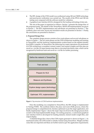
This document proposes a design procedure for a re-configurable convolutional neural network (CNN) engine for field-programmable gate array (FPGA) applications. The procedure includes developing an accurate CNN model using TensorFlow and Python, and implementing a re-configurable CNN engine from scratch using register-transfer level design. The proposed engine was synthesized for 180nm CMOS technology and achieved 96% accuracy on MNIST and CIFAR-10 datasets. A graphical user interface was also designed for loading and testing datasets on the hardware engine.

1. Citation: Kumar, P.; Ali, I.; Kim, D.-G.;
Byun, S.-J.; Kim, D.-G.; Pu, Y.-G.;
Lee, K.-Y. A Study on the Design
Procedure of Re-Configurable
Convolutional Neural Network
Engine for FPGA-Based Applications.
Electronics 2022, 11, 3883. https://
doi.org/10.3390/electronics11233883
Academic Editor: Gwanggil Jeon
Received: 21 September 2022
Accepted: 22 November 2022
Published: 24 November 2022
Publisher’s Note: MDPI stays neutral
with regard to jurisdictional claims in
published maps and institutional affil-
iations.
Copyright: © 2022 by the authors.
Licensee MDPI, Basel, Switzerland.
This article is an open access article
distributed under the terms and
conditions of the Creative Commons
Attribution (CC BY) license (https://
creativecommons.org/licenses/by/
4.0/).
electronics
Article
A Study on the Design Procedure of Re-Configurable
Convolutional Neural Network Engine for
FPGA-Based Applications
Pervesh Kumar 1, Imran Ali 1, Dong-Gyun Kim 1,2, Sung-June Byun 1,2 , Dong-Gyu Kim 3, Young-Gun Pu 1,2
and Kang-Yoon Lee 1,2,*
1 Department of Electrical and Computer Engineering, Sungkyunkwan University, Suwon 16416, Republic of Korea
2 SKAIChips, Suwon 16419, Republic of Korea
3 Department of Artificial Intelligence, Sungkyunkwan University, Suwon 16419, Republic of Korea
* Correspondence: klee@skku.edu; Tel.: +82-31-299-4954
Abstract: Convolutional neural networks (CNNs) have become a primary approach in the field of
artificial intelligence (AI), with wide range of applications. The two computational phases for every
neural network are; the training phase and the testing phase. Usually, testing is performed on high-
processing hardware engines, however, the training part is still a challenge for low-power devices.
There are several neural accelerators; such as graphics processing units and field-programmable-gate-
arrays (FPGAs). From the design perspective, an efficient hardware engine at the register-transfer
level and efficient CNN modeling at the TensorFlow level are mandatory for any type of application.
Hence, we propose a comprehensive, and step-by-step design procedure for a re-configurable CNN
engine. We used TensorFlow and Keras libraries for modeling in Python, whereas the register-transfer-
level part was performed using Verilog. The proposed idea was synthesized, placed, and routed
for 180 nm complementary metal-oxide semiconductor technology using synopsis design compiler
tools. The proposed design layout occupies an area of 3.16 × 3.16 mm2. A competitive accuracy of
approximately 96% was achieved for the Modified National Institute of Standards and Technology
(MNIST) and Canadian Institute for Advanced Research (CIFAR-10) datasets.
Keywords: deep neural network; field-programmable-gate-array (FPGA); re-synthesizable; RTL;
hardware accelerator
1. Introduction
The past decade has witnessed exponential growth in the field of artificial intelligence
(AI) owing to its promising real-time results made possible through convolutional neural
networks (CNNs). CNNs have performed exceptionally well in the field of computer vision,
such as in image classification, object recognition and natural language processing [1–4].
AI though the CNN technique is years old but it cannot gain attention due to its high
computational power requirements and the large number of complex operations involved.
Typically, a CNN is implemented using a graphical processing unit (GPU) because of
advancements in computational capabilities and the development of implementing tools
(e.g., TensorFlow, Matlab). These tools allow users to customize the CNN model according
to application requirements and deployment of multi-devices, central processing units
(CPUs) and GPUs.
Although a GPU outperforms a CPU in terms of throughput, it drains a large amount
of energy, and makes it infeasible for energy-limited resources, such as mobile devices,
embedded systems, and IoT. Contrarily, CNN implementation on field-programmable-gate-
arrays (FPGA) has shown superior results in terms of output and power efficiency, mainly
because of parallel and configurable approaches [5–7].
Electronics 2022, 11, 3883. https://doi.org/10.3390/electronics11233883 https://www.mdpi.com/journal/electronics

2. Electronics 2022, 11, 3883 2 of 13
Different approaches have different advantages and disadvantages, and FPGA is no
exception. Although the FPGA has numerous advantages, it is difficult to implement in
hardware description languages (HDL). A thorough understanding of CNN architectures,
functionality parameters, and detailed knowledge of register-transfer level (RTL) design
techniques on FPGA is required for both fixed and floating point designs. The efficient
design of a CNN engine requires many considerations, including off-board memory access
latency, on-chip memory re-usability, and high-performance arithmetic circuits [8]. Because
the computational complexity of CNN increases with the availability of reliable data, there
is a need for a re-configurable neural engine design.
There have been several attempts to reduce the gap between FPGA and CNN; how-
ever, the majority of these have focused on efficient algorithm design and performance
optimization. Some effective optimization techniques for CNN implementation on FPGA
have been proposed for creating re-configurable CNN engines. As per [9], a typical CNN
architecture is 90% of its computing convolutional layers; hence, handling convolutional
operations is a major concern. In the literature, there are several proposals for the optimiza-
tion of CNN data paths for FPGA-based designs; a detailed survey is provided in [10]. An
in-depth analysis of loop unrolling, and the loop tiling method was performed by Yufei
Ma et al., in [11]. In the proposed method the throughput of the convolutional layer’s is
improved but at the cost of more hardware. Ma et al. [12] presented an adder tree and
configurable multiplier bank based RTL compiler for various CNN architectures. The same
authors proposed an improved technique in [13] based on their earlier work in [11], using
a loop optimization technique. However, it can be deduced that their focus has been on
compiler throughput optimization in some state-of-the-art CNN models and is limited to
RTL generation by overlooking the comprehensive step from CNN modeling to training
and synthesis.
Various libraries and framework-based approaches have been proposed by several
researchers. Wang et al. [14] presented a scalable deep-learning engine with configurable
tiling sizes; however, their accelerator was designed to infer only feed-forward neural
networks. In [15], a library named Caffe was presented that automatically generates a high-
level synthesis (HLS)-based CNN engine with marginal low-level hardware optimization.
A pre-trained script description-based RTL-CNN generator was presented in [16]. In [17],
an HLS-based framework called fpgaConvNet was proposed. Similarly, a framework
called FP-DNN was proposed in [18], which automatically generates a hybrid RTL-HLS
CNN engine.
However, there are software libraries that facilitate research on AI and DL (TensorFlow,
Keras, and PyTorch). Thanks to researchers and developers, they uploaded the datasets
MNIST [19], and CIFAR-10 [20], which can be used with high-level programming languages
such as Python. The performance and energy requirements for deep learning are major
constraints, particularly in embedded systems. Hence, instead of using GPU-based energy
expensive solutions, it is important to design a power and energy-efficient re-synthesizable
hardware engine.
Building high-performance custom hardware is challenging in terms of the design
process [21–23]. The hardware architecture for such complex algorithms using low-level
HDL requires considerable time and effort. By reviewing the related literature, time
and effort can be seen in [24]. While some studies have focused on generating built-in
coefficients [25], others include training phase in hardware [26,27]. In [28], an accelerator
was designed a using Vivado HLS to speed up the analysis phase in memory which was
implemented on zynq-7000 FPGA.
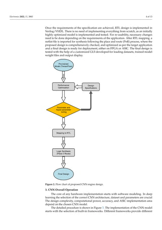
This study presents comprehensive steps for designing an FPGA-based reconfigurable
CNN engine using the latest libraries and tools in an optimized manner. The main contri-
butions are as follows:
• A compact and accurate TensorFlow-based CNN model was developed using Python
which can simulate a variety of datasets.
• Implemented a step-by-step reconfigurable CNN engine on FPGA from scratch.

3. Electronics 2022, 11, 3883 3 of 13
• The RTL design of the CNN model was synthesized using 180 nm CMOS technology
and post-layout verification was carried out. The results of the FPGA and 180 nm
testing were compared with the software model for validation.
• A graphical user interface (GUI) is designed for the loading and testing of data sets.
The rest of the paper is organized as follows: Section 2 presents the design flow of
the proposed study. The details of the TensorFlow/MATLAB implementation are given
in Section 3. The RTL implementation and sub-blocks are presented in Section 4. The
synthesis, place and route, layout and simulation results are presented in Section 5. Finally,
the conclusions are presented in Section 6.
2. Proposed Design Flow
The complete design process consists of two main phases and several sub-phases as
shown in Figure 1. The two main phases are the CNN architecture modeling and training
in TensorFlow and the hardware implementation system based on the register-transfer
level (RTL) compiler. In TensorFlow, the following two major operations are performed:
(1) CNN architecture is modeled, trained, tested, and trained weights and bias data are
saved in a .txt file; (2) input feature map data is converted into binary data, which can be
recognized by hardware tools and saved as a .txt file for further processing.
This study presents comprehensive steps for designing an FPGA-based reconfigura-
ble CNN engine using the latest libraries and tools in an optimized manner. The main
contributions are as follows.:
• A compact and accurate TensorFlow-based CNN model was developed using Py-
thon which can simulate a variety of datasets.
• Implemented a step-by-step reconfigurable CNN engine on FPGA from scratch.
• The RTL design of the CNN model was synthesized using 180 nm CMOS technology
and post-layout verification was carried out. The results of the FPGA and 180 nm
testing were compared with the software model for validation.
• A graphical user interface (GUI) is designed for the loading and testing of data sets.
The rest of the paper is organized as follows: Section 2 presents the design flow of
the proposed study. The details of the TensorFlow/MATLAB implementation are given in
Section 3. The RTL implementation and sub-blocks are presented in Section 4. The syn-
thesis, place and route, layout and simulation results are presented in Section 5. Finally,
the conclusions are presented in Section 6.
2. Proposed Design Flow
The complete design process consists of two main phases and several sub-phases as
shown in Figure 1. The two main phases are the CNN architecture modeling and training
in TensorFlow and the hardware implementation system based on the register-transfer
level (RTL) compiler. In TensorFlow, the following two major operations are performed:
(1) CNN architecture is modeled, trained, tested, and trained weights and bias data are
saved in a .txt file; (2) input feature map data is converted into binary data, which can be
recognized by hardware tools and saved as a .txt file for further processing.
Figure 1. Top structure of CNN hardware implementation.
Once the modeling was completed in TensorFlow, the RTL design is implemented in
Verilog/VHDL. The synthesis follows the place and route (PnR) process, where the pro-
posed design is comprehensively checked, optimized as per the target application, and
Define the network in TensorFlow
Train and test
Prepare for HLS
Measure and Synthesis
Explore design space (technology)
Optimized RTL implementation
Figure 1. Top structure of CNN hardware implementation.
Once the modeling was completed in TensorFlow, the RTL design is implemented
in Verilog/VHDL. The synthesis follows the place and route (PnR) process, where the
proposed design is comprehensively checked, optimized as per the target application, and
finally implemented. Figure 2 shows the major steps involved in the design process from
scratch to the final implementable design. For testing purposes, a customized graphical
user interface (GUI) is developed for loading datasets, trained model weight files, and
output display.
A detailed design flow chart of the CNN engine generator is shown in Figure 2. As
mentioned earlier, the CNN model is initially trained using TensorFlow. Weight and Bias
value files are imported and these are further tuned as per the application requirements.

4. Electronics 2022, 11, 3883 4 of 13
Once the requirements of the specification are achieved, RTL design is implemented in
Verilog/VHDL. There is no need of implementing everything from scratch, as an initially
highly optimized model is implemented and tested. For re-usability, necessary changes
need to be done depending on the requirements of the application. After RTL mapping, a
netlist file is imported for synthesis following the place and route (PnR) process, where the
proposed design is comprehensively checked, and optimized as per the target application
and a final design is ready for deployment, either on FPGA or ASIC. The final design is
tested with the help of a customized GUI developed for loading datasets, trained model
weight files and output display.
Electronics 2022, 11, x FOR PEER REVIEW 4 of 14
finally implemented. Figure 2 shows the major steps involved in the design process from
scratch to the final implementable design. For testing purposes, a customized graphical
user interface (GUI) is developed for loading datasets, trained model weight files, and
output display.
Figure 2. Flow chart of proposed CNN engine design.
A detailed design flow chart of the CNN engine generator is shown in Figure 2. As
mentioned earlier, the CNN model is initially trained using TensorFlow. Weight and Bias
value files are imported and these are further tuned as per the application requirements.
Once the requirements of the specification are achieved, RTL design is implemented in
Verilog/VHDL. There is no need of implementing everything from scratch, as an initially
highly optimized model is implemented and tested. For re-usability, necessary changes
need to be done depending on the requirements of the application. After RTL mapping, a
netlist file is imported for synthesis following the place and route (PnR) process, where
the proposed design is comprehensively checked, and optimized as per the target appli-
cation and a final design is ready for deployment, either on FPGA or ASIC. The final de-
sign is tested with the help of a customized GUI developed for loading datasets, trained
model weight files and output display.
Pre-trained
Model (TensorFlow)
Performance
Optimization
Parameter and
Hyper-parameter
tuning
HDL
Netlist
Bitfile
Weight
Mapping to RTL
Logic Synthesis
(Place n Route)
Final Design
Design
Specifcations
Figure 2. Flow chart of proposed CNN engine design.
3. CNN Overall Operation
The core of any hardware implementation starts with software modeling. In deep
learning the selection of the correct CNN architecture, dataset and parameters are crucial
The design complexity, computational power, accuracy, and ASIC implementation area
depend on the chosen CNN model.
The detailed procedure is shown in Figure 3. The implementation of the CNN model
starts with the selection of built-in frameworks. Different frameworks provide different

5. Electronics 2022, 11, 3883 5 of 13
data handling, mathematical, and graphical libraries, which are publicly available under
different licenses. For example, NumPy is the best for dataset handling, whereas Matplotlib
deals with plotting verities of graphs. For deep learning, there are three main frameworks:
Keras, PyTorch and PyCharm. This study was conducted on Keras and TensorFlow at the
backend. Once the right frame is selected, the dataset is prepared. Dozens of well-prepared
open-source datasets are available, which are good for testing purposes. Classified data,
must be prepared for the CNN. Data are not always well managed, and the accuracy of any
CNN model is highly dependent on the dataset. It is also important to have a sufficient
number of samples. A dataset that is too small, may result in over-fitting or under-fitting of
the model. Generally, a data set is split into two parts in a ratio of 80/20, where 80% of the
data are used for training and 20% are saved for testing and validation.
The core of any hardware implementation starts with software modeling. In deep
learning the selection of the correct CNN architecture, dataset and parameters are crucial
The design complexity, computational power, accuracy, and ASIC implementation area
depend on the chosen CNN model.
The detailed procedure is shown in Figure 3. The implementation of the CNN model
starts with the selection of built-in frameworks. Different frameworks provide different
data handling, mathematical, and graphical libraries, which are publicly available under
different licenses. For example, NumPy is the best for dataset handling, whereas Mat-
plotlib deals with plotting verities of graphs. For deep learning, there are three main
frameworks: Keras, PyTorch and PyCharm. This study was conducted on Keras and Ten-
sorFlow at the backend. Once the right frame is selected, the dataset is prepared. Dozens
of well-prepared open-source datasets are available, which are good for testing purposes.
Classified data, must be prepared for the CNN. Data are not always well managed, and
the accuracy of any CNN model is highly dependent on the dataset. It is also important
to have a sufficient number of samples. A dataset that is too small, may result in over-
fitting or under-fitting of the model. Generally, a data set is split into two parts in a ratio
of 80/20, where 80% of the data are used for training and 20% are saved for testing and
validation.
Figure 3. Implementation flow of the proposed CNN engine.
Once the data are ready, the next step is model training which is the most crucial
step. Training is an iterative process, which involves complex mathematical computa-
tions. Training has two major operations: forward propagation and backpropagation. In
forward propagation, starting from the input data, the weight and bias values are con-
volved and forward propagated to the next operational layer, adding weight and bias
values untill the final SoftMax layer. Forward propagation involves several layer-wise op-
erations; that is, convolutional, pooling (max or average), activation, and dense layers.
Each layer-wise operation is discussed in detail in the following section. Forward propa-
gation is followed by backpropagation.
Back-propagation computes the gradient of the loss function with respect to weight
using the chain rule. In supervised learning, the output vector is generated from input
6. Extract
Weight and
Bias Values
2. Prepare Dataset
Training Data
Test Data
Validation Data
1. Select Library
TensorFlow
Keras
PyTorch
Training
(Back &
Forward
Propagation)
4. Model Training
Parameters Tuning
3. CNN Model
No. of Kernels
Kernel size
No. of Layers
5. Trained Model Validation
Model
Validation
Review Results
(accuracy)
Figure 3. Implementation flow of the proposed CNN engine.
Once the data are ready, the next step is model training which is the most crucial
step. Training is an iterative process, which involves complex mathematical computations.
Training has two major operations: forward propagation and backpropagation. In forward
propagation, starting from the input data, the weight and bias values are convolved and
forward propagated to the next operational layer, adding weight and bias values untill
the final SoftMax layer. Forward propagation involves several layer-wise operations; that
is, convolutional, pooling (max or average), activation, and dense layers. Each layer-wise
operation is discussed in detail in the following section. Forward propagation is followed
by backpropagation.
Back-propagation computes the gradient of the loss function with respect to weight
using the chain rule. In supervised learning, the output vector is generated from input
vectors, and an error/loss is generated if the desired output is not achieved. The parameters
(weights/bias) values are adjusted to achieve the best output results. Computing the
gradient layer-by-layer, and iterating backward from the last layer to avoid redundant
computation of intermediate terms in the chain rule.
Backpropagation error = achieved output − targeted output
Each stage is explained in detail, in the following steps.

6. Electronics 2022, 11, 3883 6 of 13
3.1. Uploading the Dataset
The MNIST/CIFAR10 and other open datasets are available for learning. In this study,
we used the MNIST dataset. Once the dataset is successfully loaded, 4 random samples are
printed for confirmation purposes shown in Figure 4.
vectors, and an error/loss is generated if the desired output is not achieved. The parame-
ters (weights/bias) values are adjusted to achieve the best output results. Computing the
gradient layer-by-layer, and iterating backward from the last layer to avoid redundant
computation of intermediate terms in the chain rule.
Backpropagation error = 𝑎𝑐ℎ𝑖𝑒𝑣𝑒𝑑 𝑜𝑢𝑡𝑝𝑢𝑡 − 𝑡𝑎𝑟𝑔𝑒𝑡𝑒𝑑 𝑜𝑢𝑡𝑝𝑢𝑡
Each stage is explained in detail, in the following steps.
3.1. Uploading the Dataset
The MNIST/CIFAR10 and other open datasets are available for learning. In this
study, we used the MNIST dataset. Once the dataset is successfully loaded, 4 random
samples are printed for confirmation purposes shown in Figure 4.
Figure 4. Dataset download and printing of random samples.
3.2. Divide the Dataset into Test/Training Dataset
Once the dataset is loaded/downloaded, it must be split into two sets: the training
and test datasets. Usually, the 80/20 ratio is used. Figure 5 shows the divided datasets.
Figure 5. Dividing the dataset into Training and Test datasets.
3.3. Define the CNN Architecture
The definition of the CNN architecture contains comprehensive details of the param-
eters and hyper-parameters. Information on the number of convolutional layers, fully con-
nected layers, number of kernels, kernel size, pooling type, pooling size, stride window,
activation function, number of epochs, batch size, learning rate, and use of bias infor-
mation is provided. The selection of parameters is shown in Figure 6.
Figure 4. Dataset download and printing of random samples.
3.2. Divide the Dataset into Test/Training Dataset
Once the dataset is loaded/downloaded, it must be split into two sets: the training
and test datasets. Usually, the 80/20 ratio is used. Figure 5 shows the divided datasets.
ters (weights/bias) values are adjusted to achieve the best output results. Computing the
gradient layer-by-layer, and iterating backward from the last layer to avoid redundant
computation of intermediate terms in the chain rule.
Backpropagation error = 𝑎𝑐ℎ𝑖𝑒𝑣𝑒𝑑 𝑜𝑢𝑡𝑝𝑢𝑡 − 𝑡𝑎𝑟𝑔𝑒𝑡𝑒𝑑 𝑜𝑢𝑡𝑝𝑢𝑡
Each stage is explained in detail, in the following steps.
3.1. Uploading the Dataset
The MNIST/CIFAR10 and other open datasets are available for learning. In this
study, we used the MNIST dataset. Once the dataset is successfully loaded, 4 random
samples are printed for confirmation purposes shown in Figure 4.
Figure 4. Dataset download and printing of random samples.
3.2. Divide the Dataset into Test/Training Dataset
Once the dataset is loaded/downloaded, it must be split into two sets: the training
and test datasets. Usually, the 80/20 ratio is used. Figure 5 shows the divided datasets.
Figure 5. Dividing the dataset into Training and Test datasets.
3.3. Define the CNN Architecture
The definition of the CNN architecture contains comprehensive details of the param-
eters and hyper-parameters. Information on the number of convolutional layers, fully con-
nected layers, number of kernels, kernel size, pooling type, pooling size, stride window,
activation function, number of epochs, batch size, learning rate, and use of bias infor-
mation is provided. The selection of parameters is shown in Figure 6.
Figure 5. Dividing the dataset into Training and Test datasets.
3.3. Define the CNN Architecture
The definition of the CNN architecture contains comprehensive details of the param-
eters and hyper-parameters. Information on the number of convolutional layers, fully
connected layers, number of kernels, kernel size, pooling type, pooling size, stride window,
activation function, number of epochs, batch size, learning rate, and use of bias information
is provided. The selection of parameters is shown in Figure 6.
3.4. Output Accuracy Optimization
Once the CNN architecture is selected, it is compiled before the training starts. In this
step, we define the loss function, optimizer and metrics. After the fit function measures,
the performance of CNN model is determined. Fitting refers to adjusting the parameters in
the model to improve accuracy, as shown in Figure 7.
3.5. Saving the Trained Model and Weight Values
The model can be saved after and during the training. This means that we can resume
if it is left incomplete for any reason. A replica of the model can be created using the saved

7. Electronics 2022, 11, 3883 7 of 13
model and weight file. In this study, we loaded the saved weight values for hardware
processing. The saving commands are shown in Figure 8.
Electronics 2022, 11, x FOR PEER REVIEW 7
Figure 6. Definition of parameters.
3.4. Output Accuracy Optimization
Once the CNN architecture is selected, it is compiled before the training starts. In
step, we define the loss function, optimizer and metrics. After the fit function meas
the performance of CNN model is determined. Fitting refers to adjusting the param
in the model to improve accuracy, as shown in Figure 7.
Figure 7. Selection of optimizer and loss function for output accuracy tuning.
3.5. Saving the Trained Model and Weight Values
The model can be saved after and during the training. This means that we can res
if it is left incomplete for any reason. A replica of the model can be created using the s
model and weight file. In this study, we loaded the saved weight values for hardw
processing. The saving commands are shown in Figure 8.
Figure 8. Commands for saving trained model and weight files.
4. CNN: Layerwise Implementation
4.1. Proposed Top CNN Engine
Our aim is to present a power-efficient design implementation technique that
not compromise the CNN structure and accuracy. The CNN engine is the most freque
used system for all applications, and thus consumes more power. The top CNN engi
shown in Figure 9, where the power consumption is reduced by reusing the mem
Figure 6. Definition of parameters.
Electronics 2022, 11, x FOR PEER REVIEW 7 of 14
Figure 6. Definition of parameters.
3.4. Output Accuracy Optimization
Once the CNN architecture is selected, it is compiled before the training starts. In this
step, we define the loss function, optimizer and metrics. After the fit function measures,
the performance of CNN model is determined. Fitting refers to adjusting the parameters
in the model to improve accuracy, as shown in Figure 7.
Figure 7. Selection of optimizer and loss function for output accuracy tuning.
3.5. Saving the Trained Model and Weight Values
The model can be saved after and during the training. This means that we can resume
if it is left incomplete for any reason. A replica of the model can be created using the saved
model and weight file. In this study, we loaded the saved weight values for hardware
processing. The saving commands are shown in Figure 8.
Figure 8. Commands for saving trained model and weight files.
4. CNN: Layerwise Implementation
4.1. Proposed Top CNN Engine
Our aim is to present a power-efficient design implementation technique that does
not compromise the CNN structure and accuracy. The CNN engine is the most frequently
used system for all applications, and thus consumes more power. The top CNN engine is
shown in Figure 9, where the power consumption is reduced by reusing the memory,
Figure 7. Selection of optimizer and loss function for output accuracy tuning.
Figure 6. Definition of parameters.
3.4. Output Accuracy Optimization
Once the CNN architecture is selected, it is compiled before the training starts. In this
step, we define the loss function, optimizer and metrics. After the fit function measures,
the performance of CNN model is determined. Fitting refers to adjusting the parameters
in the model to improve accuracy, as shown in Figure 7.
Figure 7. Selection of optimizer and loss function for output accuracy tuning.
3.5. Saving the Trained Model and Weight Values
The model can be saved after and during the training. This means that we can resume
if it is left incomplete for any reason. A replica of the model can be created using the saved
model and weight file. In this study, we loaded the saved weight values for hardware
processing. The saving commands are shown in Figure 8.
Figure 8. Commands for saving trained model and weight files.
4. CNN: Layerwise Implementation
4.1. Proposed Top CNN Engine
Our aim is to present a power-efficient design implementation technique that does
not compromise the CNN structure and accuracy. The CNN engine is the most frequently
used system for all applications, and thus consumes more power. The top CNN engine is
shown in Figure 9, where the power consumption is reduced by reusing the memory,
Figure 8. Commands for saving trained model and weight files.
4. CNN: Layerwise Implementation
4.1. Proposed Top CNN Engine
Our aim is to present a power-efficient design implementation technique that does
not compromise the CNN structure and accuracy. The CNN engine is the most frequently
used system for all applications, and thus consumes more power. The top CNN engine is
shown in Figure 9, where the power consumption is reduced by reusing the memory, which
occupies a major portion of the CNN engine. We applied the memory re-use technique, in
which the input feature buffer memory was re-used for storing the updated weights values
after each iteration.
4.2. Convolutional Layer
The convolutional layer is used to identify the primary features in the image by
convolving with a set of learnable filters. Convolution is a linear and simple multiplication
operation of a single or multi-dimensional array vector called filters with an input array.
The filter’s dimensions are significantly small (3 × 3, 5 × 5, or 7 × 7) as compared to the
input data dimension. Each filter is convolved horizontally and vertically in a sliding

8. Electronics 2022, 11, 3883 8 of 13
window fashion with input data resulting in an array of feature maps. The number of
features maps is equal to the number of convolved filters. The detailed CNN architecture is
shown in Figure 10. The element-wise multiplication and summation operations are given
in Equation (1).
Electronics 2022, 11, x FOR PEER REVIEW 8 of 14
which occupies a major portion of the CNN engine. We applied the memory re-use tech-
nique, in which the input feature buffer memory was re-used for storing the updated
weights values after each iteration.
Figure 9. Top architecture of the proposed CNN engine.
4.2. Convolutional Layer
The convolutional layer is used to identify the primary features in the image by con-
volving with a set of learnable filters. Convolution is a linear and simple multiplication
operation of a single or multi-dimensional array vector called filters with an input array.
The filter’s dimensions are significantly small (3 × 3, 5 × 5, or 7 × 7) as compared to the
input data dimension. Each filter is convolved horizontally and vertically in a sliding win-
dow fashion with input data resulting in an array of feature maps. The number of features
maps is equal to the number of convolved filters. The detailed CNN architecture is shown
in Figure 10. The element-wise multiplication and summation operations are given in
Equation (1).
𝑃 = 𝑅 × 𝐶 × 𝑀 + 𝐵 (1)
During the mathematical operation, a bias term was added to the sum of the
weighted input. The following equation shows the calculation of the output feature map.
𝑂𝑢𝑡𝑝𝑢𝑡 =
𝐼𝑛𝑝𝑢𝑡 − 𝐹𝑖𝑙𝑡𝑒𝑟 + 2 × 𝑃𝑎𝑑𝑑𝑖𝑛𝑔
𝑆𝑡𝑟𝑖𝑑𝑒
+ 𝐵𝑖𝑎𝑠 (2)
where padding is the optional number of pixel values added to maintain the optimal di-
mension. When an image is convolved with filters, and the stride slides the filters with a
certain number of pixels across the input array, sliding windows are fixed according to
the output results.
3
3
32
4
29
32x32
29x29x4
3
CONV layer C1 + ReLU Max Pool Layer L2 Max Pool Layer P4 Flatten
32
1
2
3
4
29
4
14
1
2
3
4
14x14x4
14
1
2
3
4
11x11x4
11
2
4
1
2
3
4
4
11
3
3
1
1
2
3
4
1
2
3
4
5x5x4
5
5
CONV layer C3 + ReLU
FC5
1
2
3
0
9
5
4
• Convolutional Layer: E = (H+2xP-R)/S +1
• Pooling Layer: E = (H - R)/S +1
• R: Filter Size
• C: Number of Channels
• M: Number of Filters
• S: Stride
• P: Padding
• B: Bias
• H: Input Image Size
• E: Output Image Size
100 16
• Parameter: Pc = R2
xCL-1xM+B
Figure 10. Detailed CNN architecture.
4.3. Pooling Layer and Activation Function
The pooling layer works similar to the convolutional layer. This diminishes the spa-
tial size of convolved features. Moreover, it aids in dimension reduction during dominant
feature extraction to achieve the highest recognition accuracy. Pooling operation can be
Output
Weight
Buffer
ReLU Pooling
CNN Layer
Input
Data
Weight
and Bias
Top Controller
Data
Weight
Adder
Tree
Input
Weight
Buffer
Figure 9. Top architecture of the proposed CNN engine.
Pc = R2
× CL−1 × M + B (1)
Figure 9. Top architecture of the proposed CNN engine.
4.2. Convolutional Layer
The convolutional layer is used to identify the primary features in the image by con-
volving with a set of learnable filters. Convolution is a linear and simple multiplication
operation of a single or multi-dimensional array vector called filters with an input array.
The filter’s dimensions are significantly small (3 × 3, 5 × 5, or 7 × 7) as compared to the
input data dimension. Each filter is convolved horizontally and vertically in a sliding win-
dow fashion with input data resulting in an array of feature maps. The number of features
maps is equal to the number of convolved filters. The detailed CNN architecture is shown
in Figure 10. The element-wise multiplication and summation operations are given in
Equation (1).
𝑃 = 𝑅 × 𝐶 × 𝑀 + 𝐵 (1)
During the mathematical operation, a bias term was added to the sum of the
weighted input. The following equation shows the calculation of the output feature map.
𝑂𝑢𝑡𝑝𝑢𝑡 =
𝐼𝑛𝑝𝑢𝑡 − 𝐹𝑖𝑙𝑡𝑒𝑟 + 2 × 𝑃𝑎𝑑𝑑𝑖𝑛𝑔
𝑆𝑡𝑟𝑖𝑑𝑒
+ 𝐵𝑖𝑎𝑠 (2)
where padding is the optional number of pixel values added to maintain the optimal di-
mension. When an image is convolved with filters, and the stride slides the filters with a
certain number of pixels across the input array, sliding windows are fixed according to
the output results.
3
3
32
4
29
32x32
29x29x4
3
CONV layer C1 + ReLU Max Pool Layer L2 Max Pool Layer P4 Flatten
32
1
2
3
4
29
4
14
1
2
3
4
14x14x4
14
1
2
3
4
11x11x4
11
2
4
1
2
3
4
4
11
3
3
1
1
2
3
4
1
2
3
4
5x5x4
5
5
CONV layer C3 + ReLU
FC5
1
2
3
0
9
5
4
• Convolutional Layer: E = (H+2xP-R)/S +1
• Pooling Layer: E = (H - R)/S +1
• R: Filter Size
• C: Number of Channels
• M: Number of Filters
• S: Stride
• P: Padding
• B: Bias
• H: Input Image Size
• E: Output Image Size
100 16
• Parameter: Pc = R2
xCL-1xM+B
Figure 10. Detailed CNN architecture.
4.3. Pooling Layer and Activation Function
The pooling layer works similar to the convolutional layer. This diminishes the spa-
tial size of convolved features. Moreover, it aids in dimension reduction during dominant
feature extraction to achieve the highest recognition accuracy. Pooling operation can be
Top Controller
Figure 10. Detailed CNN architecture.
During the mathematical operation, a bias term was added to the sum of the weighted
input. The following equation shows the calculation of the output feature map.
Outputsize =
Inputwidth − Filtersize + 2 × Padding
Stride
+ Bias (2)
where padding is the optional number of pixel values added to maintain the optimal
dimension. When an image is convolved with filters, and the stride slides the filters with a
certain number of pixels across the input array, sliding windows are fixed according to the
output results.
4.3. Pooling Layer and Activation Function
The pooling layer works similar to the convolutional layer. This diminishes the spatial
size of convolved features. Moreover, it aids in dimension reduction during dominant
feature extraction to achieve the highest recognition accuracy. Pooling operation can be
performed in two ways: average pooling and maximum pooling. Maximum pooling.
Maximum pooling takes the dominant pixel value from the chosen pooling windows,
whereas, average pooling takes the average of the selected pooling window. Both methods
ultimately result in a dimension reduction.
After calculation the weighted sum and bias values, the activation function determines
whether to fire a neuron, which is the same as checking the threshold. The primary aim
of the activation function is to add non-linearity to the output. A neural network without
an activation function is similar to linear regression problem, which does not support
complex mathematical operations. In summary, an activation function improves the neural

9. Electronics 2022, 11, 3883 9 of 13
network by learning and performing complex functions. The most widely used activation
functions are sigmoid, ReLU, and Tanh [29]. These functions optimize the detection rate of
CNN, however, they are rarely used in real world applications, to be exact on hardware, as
memory is limited.
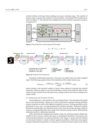
4.4. Fully Connected Layer
The final output from the convolution and pooling operations is followed a by flattened
layer. The fully connected (FC) layer works like a layer of the multi-layer perceptron and
consists of more than one FC layer. The final output of the entire convolutional operation
is saved in a single-column vector. Each value in the column indicates the probability
that the features match the label. The FC layer is used to convert the images into labels
based on the learned features from the convolutional process. Each neuron carries certain
probability value. The neuron with the highest probability value is declared the output,
and the corresponding label classifies that particular class.
5. Synthesis and Results
The design compiler tool is the core of Synopsys synthesis products. It optimizes the
design for the area and power-efficient local representation of given blocks. The design
compiler consists of hardware description language (HDL) design synthesis tools that
optimize gate-level designs. Both combinational and sequential designs can be optimized
for speed, power, and area.
Figure 5 shows the steps to be followed for the synthesis with the design compiler.
These steps include reading the VHDL/Verilog source file in the design, applying the
constraints as per the specification, and design optimization. The reading of HDL design
involved two tasks. First, the command analysis checks the syntactical errors, creates
libraries, and saves the HDL intermediate files at a specified location. The second task is
command elaboration, which translates intermediate files into a technology-independent
design produced during the analysis. In the elaboration report, we can see the number and
types of memory elements. If the elaboration is completed successfully, the next step is the
constraints defining. Constraints are the set of parameters that the designer provides to a
design compiler in order to limit the operations the synthesis tool can or cannot perform
with the design and its behavior.
Figure 11 shows the synthesized layout of the proposed CNN engine, following the
steps presented in this manuscript. It was synthesized for a 180 nm CMOS process using
a design compiler and IC compiler. It occupies a 3.16 mm × 3.16 mm die area. To verify
the proposed design procedure, we tested our design using open-source datasets MNIST,
CIFAR-10, and STL-10, as shown in Table 1. A comparison with other state-of-art proposed
designs is presented in Table 2. Most of the proposed ideas are limited to FPGAs. The
proposed procedure covers both software and hardware implementations, and synthesis
up to the ASIC level.
Table 1. Tested Dataset.
Dataset Type Size Classes
MNIST Gray 28–28 10
CIFAR-10 Color 32 × 32 10
STL-10 Color 96 × 96 10
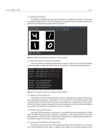
A customized controller-based GUI was developed for testing, as shown in Figure 12.
It was used to load the pre-trained weight and bias values files, and input data for testing.
This GUI has many other control options, such as enable, reset, read, and write. Using
this GUI, we can verify the output after each convolutional layer. To read and write, the
files must be saved within a particular system path, where they can load to read or save to
write. It reads the test simple pixel value in vector form, and weights values in hexadecimal.
The final output class field is marked as the ANIC Class, which shows the final output

10. Electronics 2022, 11, 3883 10 of 13
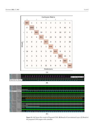
class after the test. The tensor flow modeling results are shown in Figure 13a, in which
we achieved the precision score of approximately 96. The proposed CNN engine design
procedure was verified at the RTL level as shown in Figure 13b,c. It correctly classified the
data as classified in the GUI.
Table 2. Performance comparison with related works.
Parameters Our Work [18] [21]
Technology CMOS 180 FPGA (Virtex-7) Zynq XC7Z045
Precision 16–32 fixed 16 fixed 16 fixed
Gate Count 323,210 164,100 -
Memory Utilization 58% 67% 65%
Clock Frequency 250 Hz 150 Hz 150 Hz
GOPS 210 364.4 137.0
Electronics 2022, 11, x FOR PEER REVIEW 10 of 14
Figure 11. Layout of the proposed CNN engine.
Table 1. Tested Dataset.
Dataset Type Size Classes
MNIST Gray 28–28 10
CIFAR-10 Color 32 × 32 10
STL-10 Color 96 × 96 10
Table 2. Performance comparison with related works.
Parameters Our Work [18] [21]
Technology CMOS 180 FPGA (Virtex-7) Zynq XC7Z045
Precision 16–32 fixed 16 fixed 16 fixed
Gate Count 323,210 164,100 -
Memory Utilization 58% 67% 65%
Clock Frequency 250 Hz 150 Hz 150 Hz
GOPS 210 364.4 137.0
A customized controller-based GUI was developed for testing, as shown in Figure
12. It was used to load the pre-trained weight and bias values files, and input data for
testing. This GUI has many other control options, such as enable, reset, read, and write.
Using this GUI, we can verify the output after each convolutional layer. To read and write,
Figure 11. Layout of the proposed CNN engine.
Electronics 2022, 11, x FOR PEER REVIEW 11 of 14
Figure 12. A customized GUI for testing.
Figure 12. A customized GUI for testing.

11. Electronics 2022, 11, 3883 11 of 13
Figure 12. A customized GUI for testing.
(A)
(B)
Electronics 2022, 11, x FOR PEER REVIEW 12 of 14
(C)
Figure 13. (A) Tensor flow result of Proposed CNN. (B) Result of Convolutional Layer. (C) Result
of the proposed CNN engine with controller.
6. Conclusions
In this study, an SW/HW co-design procedure is presented for designing a CNN en-
gine to fill the gap owing to its fast growth and lower power re-configurable FPGA-based
applications. This was achieved by proposing a detailed design procedure for a customi-
zable and re-configurable CNN engine.
Figure 13. (A) Tensor flow result of Proposed CNN. (B) Result of Convolutional Layer. (C) Result of
the proposed CNN engine with controller.

12. Electronics 2022, 11, 3883 12 of 13
6. Conclusions
In this study, an SW/HW co-design procedure is presented for designing a CNN
engine to fill the gap owing to its fast growth and lower power re-configurable FPGA-
based applications. This was achieved by proposing a detailed design procedure for a
customizable and re-configurable CNN engine.
Additionally, any user can generate as many FPGA-based CNN models as possible
without starting every time from the very scratch, through slight modifications as per the
application requirements and following the detailed steps. With a given framework, a user
can integrate new layers for modern CNN models and add features to the existing layers.
All RTL blocks are hand-coded in Verilog; thus FPGA (Altera, Xilinx) implementation and
verification are handy. All CNN models can be easily processed for the ASIC implementa-
tions. The design process used TensorFlow and MATLAB to train and test the CNN model
before implementation. The proposed design idea was validated on different data sets
(MNIST and, CIFAR-10) and competitive results were achieved. A customized GUI makes
it easier to perform testing with simple clicks. Furthermore, the proposed design procedure
achieved considerable accuracy.
Author Contributions: Conceptualization, P.K.; methodology, P.K. and I.A.; software, P.K. and I.A.;
validation, investigation P.K. and I.A.; resources D.-G.K. (Dong-Gyu Kim); data curation, S.-J.B. and
D.-G.K. (Dong-Gyun Kim); writing—draft presentation, P.K.; writing—review and editing, P.K. and
K.-Y.L.; supervision, K.-Y.L., I.A. and Y.-G.P.; project administration, K.-Y.L.; funding acquisition,
K.-Y.L. All authors have read and agreed to the published version of the manuscript.
Funding: This work was supported by Institute of Information & communications Technology
Planning & Evaluation (IITP) grant funded by the Republic of Korea government(MSIT) (No. 2019-
0-00421, Artificial Intelligence Graduate School Program(Sungkyunkwan University)) and was
supported by the MSIT (Ministry of Science and ICT), Republic of Korea, under the ICT Creative
Consilience Program (IITP-2022-2020-0-01821) supervised by the IITP (Institute for Information &
communications Technology Planning & Evaluation).
Conflicts of Interest: The authors declare no conflict of interest.
References
1. Lecun, Y.; Bottou, L.; Bengio, Y.; Haffner, P. Gradient-based learning applied to document recognition. Proc. IEEE 1998, 86,
2278–2324. [CrossRef]
2. Verma, N.K.; Sharma, T.; Rajurkar, S.D.; Salour, A. Object identification for inventory management using convolutional neural
network. In Proceedings of the 2016 IEEE Applied Imagery Pattern Recognition Workshop (AIPR), Washington, DC, USA, 18–20
October 2020; pp. 1–6.
3. LeCun, Y.; Boser, B.; Denker, J.S.; Henderson, D.; Howard, R.E.; Hubbard, W.; Jackel, L.D. Backpropagation Applied to
Handwritten Zip Code Recognition. Neural Comput. 1989, 1, 541–551. [CrossRef]
4. Yadav, S.S.; Jadhav, S.M. Deep convolutional neural network based medical image classification for disease diagnosis. J. Big Data
2019, 6, 113. [CrossRef]
5. Asano, S.; Maruyama, T.; Yamaguchi, Y. Performance comparison of FPGA, GPU and CPU in image processing. In Proceedings
of the 2009 International Conference on Field Programmable Logic and Applications, Prague, Czech Republic, 31 August–2
September 2009; pp. 126–131.
6. Mousouliotis, P.G.; Petrou, L.P. CNN-Grinder: From Algorithmic to High-Level Synthesis descriptions of CNNs for Low-end-
low-cost FPGA SoCs. Microprocess. Microsyst. 2020, 73, 102990. [CrossRef]
7. Lacey, G.; Taylor, G.W.; Areibi, S. Deep learning on FPGAs: Past, present, and future. arXiv 2006, arXiv:1602.04283.
8. Shawahna, A.; Sait, S.M.; El-Maleh, A. FPGA-based accelerators of deep learning networks for learning and classification: A
review. IEEE Access 2019, 7, 7823–7859. [CrossRef]
9. Cong, J.; Xiao, B. Minimizing computation in convolutional neural networks. In Artificial Neural Networks and Machine Learning–
ICANN 2014, Proceedings of the 24th International Conference on Artificial Neural Networks (ICANN 2014), Hamburg, Germany, 15–19
September 2014; Springer International Publishing: Cham, Switzerland, 2014; pp. 281–290.
10. Abdelouahab, K.; Pelcat, M.; Serot, J.; Berry, F. Accelerating CNN inference on FPGAs: A survey. arXiv 2018, arXiv:1806.01683.
11. Ma, Y.; Cao, Y.; Vrudhula, S.; Seo, J.S. Optimizing loop operation and dataflow in FPGA acceleration of deep convolutional
neural networks. In FPGA ‘17: Proceedings of the 2017 ACM/SIGDA International Symposium on Field-Programmable Gate Arrays,
Proceedings of the 2017 ACM/SIGDA International Symposium on Field-Programmable Gate Arrays, Monterey, CA, USA, 22–24 February
2017; Association for Computing Machinery: New York, NY, USA, 2017; pp. 45–54.

13. Electronics 2022, 11, 3883 13 of 13
12. Ma, Y.; Suda, N.; Cao, Y.; Seo, J.S.; Vrudhula, S. Scalable and modularized RTL compilation of convolutional neural networks onto
FPGA. In Proceedings of the 2016 26th International Conference on Field Programmable Logic and Applications (FPL), Lausanne,
Switzerland, 29 August–2 September 2016; pp. 1–8.
13. Ma, Y.; Cao, Y.; Vrudhula, S.; Seo, J.S. An automatic RTL compiler for high-throughput FPGA implementation of diverse deep
convolutional neural networks. In Proceedings of the 2017 27th International Conference on Field Programmable Logic and
Applications (FPL), Ghent, Belgium, 4–8 September 2017; pp. 1–8.
14. Wang, C.; Gong, L.; Yu, Q.; Li, X.; Xie, Y.; Zhou, X. DLAU: A scalable deep learning accelerator unit on FPGA. IEEE Trans. Comput.
Aided Des. Integr. Circuits Syst. 2017, 36, 513–517. [CrossRef]
15. Aghdam, H.H.; Heravi, E.J. Caffe Library. In Guide to Convolutional Neural Networks; Springer International Publishing: Cham,
Switzerland, 2017; pp. 131–166. [CrossRef]
16. Rivera-Acosta, M.; Ortega-Cisneros, S.; Rivera, J. Automatic Tool for Fast Generation of Custom Convolutional Neural Networks
Accelerators for FPGA. Electronics 2019, 8, 641. [CrossRef]
17. Venieris, S.I.; Bouganis, C.-S. fpgaConvNet: A framework for mapping convolutional neural networks on FPGAs. In Proceed-
ings of the 2016 IEEE 24th Annual International Symposium on Field-Programmable Custom Computing Machines (FCCM),
Washington, DC, USA, 1–3 May 2016; pp. 40–47.
18. Guan, Y.; Liang, H.; Xu, N.; Wang, W.; Shi, S.; Chen, X.; Sun, G.; Zhang, W.; Cong, J. FP-DNN: An automated framework for
mapping deep neural networks onto FPGAs with RTL-HLS hybrid templates. In Proceedings of the 2017 IEEE 25th Annual
International Symposium on Field-Programmable Custom Computing Machines (FCCM), Napa, CA, USA, 30 April–2 May 2017;
pp. 152–159.
19. Deng, L. The MNIST Database of Handwritten Digit Images for Machine Learning Research [Best of the Web]. IEEE Signal Process.
Mag. 2012, 29, 141–142. [CrossRef]
20. Krizhevsky, A.; Hinton, G. Learning Multiple Layers of Features from Tiny Images. 2009. Available online: http://www.cs.
utoronto.ca/~{}kriz/learning-features-2009-TR.pdf (accessed on 15 November 2022).
21. Russakovsky, O.; Deng, J.; Su, H.; Krause, J.; Satheesh, S.; Ma, S.; Huang, Z.; Karpathy, A.; Khosla, A.; Bernstein, M.; et al.
ImageNet Large Scale Visual Recognition Challenge. Int. J. Comput. Vis. 2015, 115, 211–252. [CrossRef]
22. Byun, S.-J.; Kim, D.-G.; Park, K.-D.; Choi, Y.-J.; Kumar, P.; Ali, I.; Kim, D.-G.; Yoo, J.-M.; Huh, H.-K.; Jung, Y.-J.; et al. A Low-Power
Analog Processor-in-Memory-Based Convolutional Neural Network for Biosensor Applications. Sensors 2022, 22, 4555. [CrossRef]
[PubMed]
23. Kumar, P.; Yingge, H.; Ali, I.; Pu, Y.-G.; Hwang, K.-C.; Yang, Y.; Jung, Y.-J.; Huh, H.-K.; Kim, S.-K.; Yoo, J.-M.; et al. A Configurable
and Fully Synthesizable RTL-Based Convolutional Neural Network for Biosensor Applications. Sensors 2022, 22, 2459. [CrossRef]
[PubMed]
24. Moolchandani, D.; Kumar, A.; Sarangi, S.R. Accelerating CNN Inference on ASICs: A Survey. J. Syst. Arch. 2020, 113, 101887.
[CrossRef]
25. Alzubaidi, L.; Zhang, J.; Humaidi, A.J.; Al-Dujaili, A.; Duan, Y.; Al-Shamma, O.; Santamaría, J.; Fadhel, M.A.; Al-Amidie, M.;
Farhan, L. Review of deep learning: Concepts, CNN architectures, challenges, applications, future directions. J. Big Data 2021,
8, 53. [CrossRef]
26. Nazemi, M.; Eshratifar, A.E.; Pedram, M. A hardware-friendly algorithm for scalable training and deployment of dimensionality
reduction models on FPGA. In Proceedings of the 2018 19th International Symposium on Quality Electronic Design (ISQED),
Santa Clara, CA, USA, 13–14 March 2018; pp. 395–400.
27. He, X.; Lu, W.; Yan, G.; Zhang, X. Joint Design of Training and Hardware Towards Efficient and Accuracy-Scalable Neural
Network Inference. IEEE J. Emerg. Sel. Top. Circuits Syst. 2018, 8, 810–821. [CrossRef]
28. Li, C.; Bi, Y.; Benezeth, Y.; Ginhac, D.; Yang, F. High-level synthesis for FPGAs: Code optimization strategies for real-time image
processing. J. Real Time Image Process. 2017, 14, 701–712. [CrossRef]
29. Layer Activation Functions. Keras Website. Available online: https://keras.io/api/layers/activations/ (accessed on 15 November 2022).