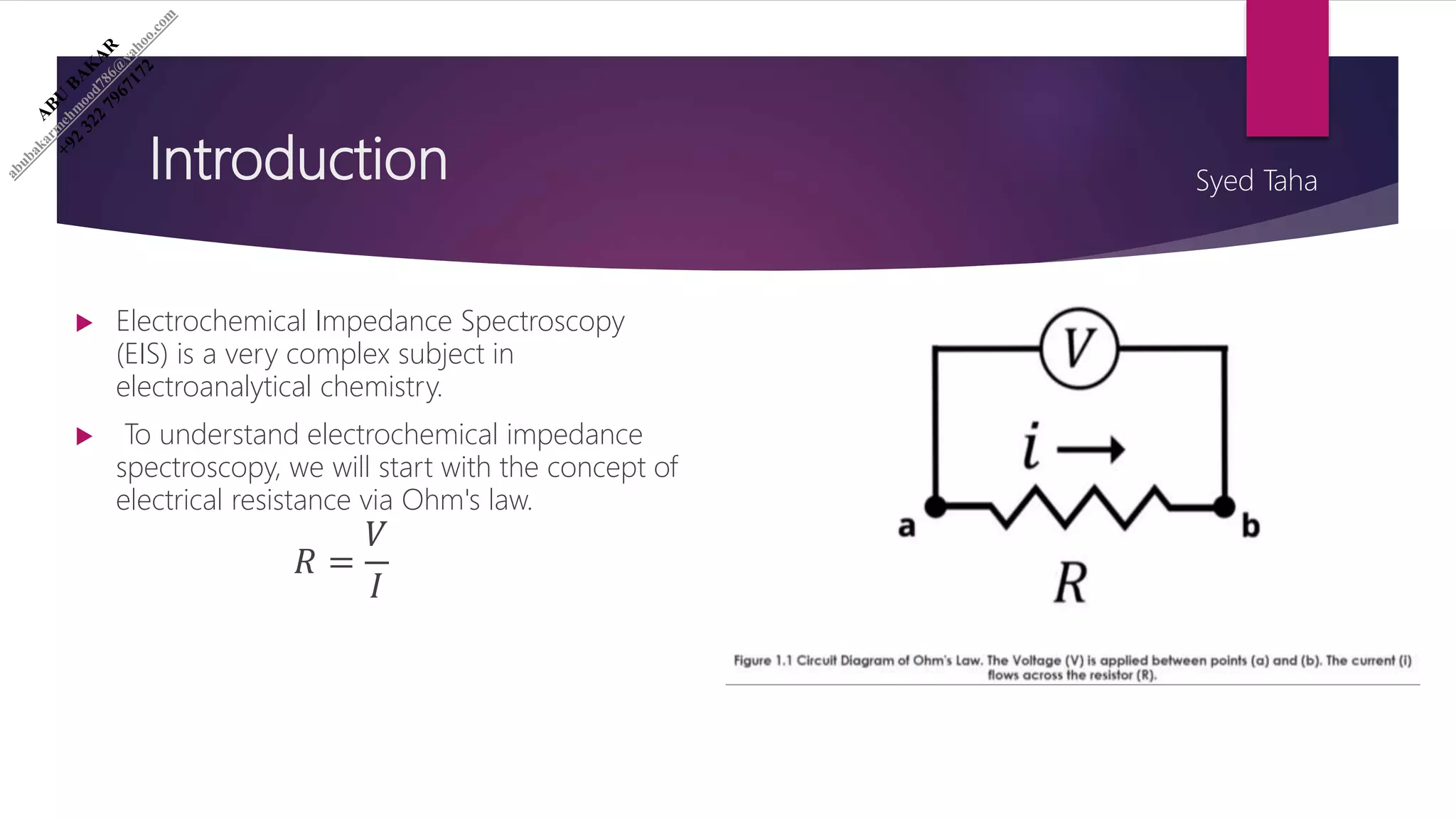
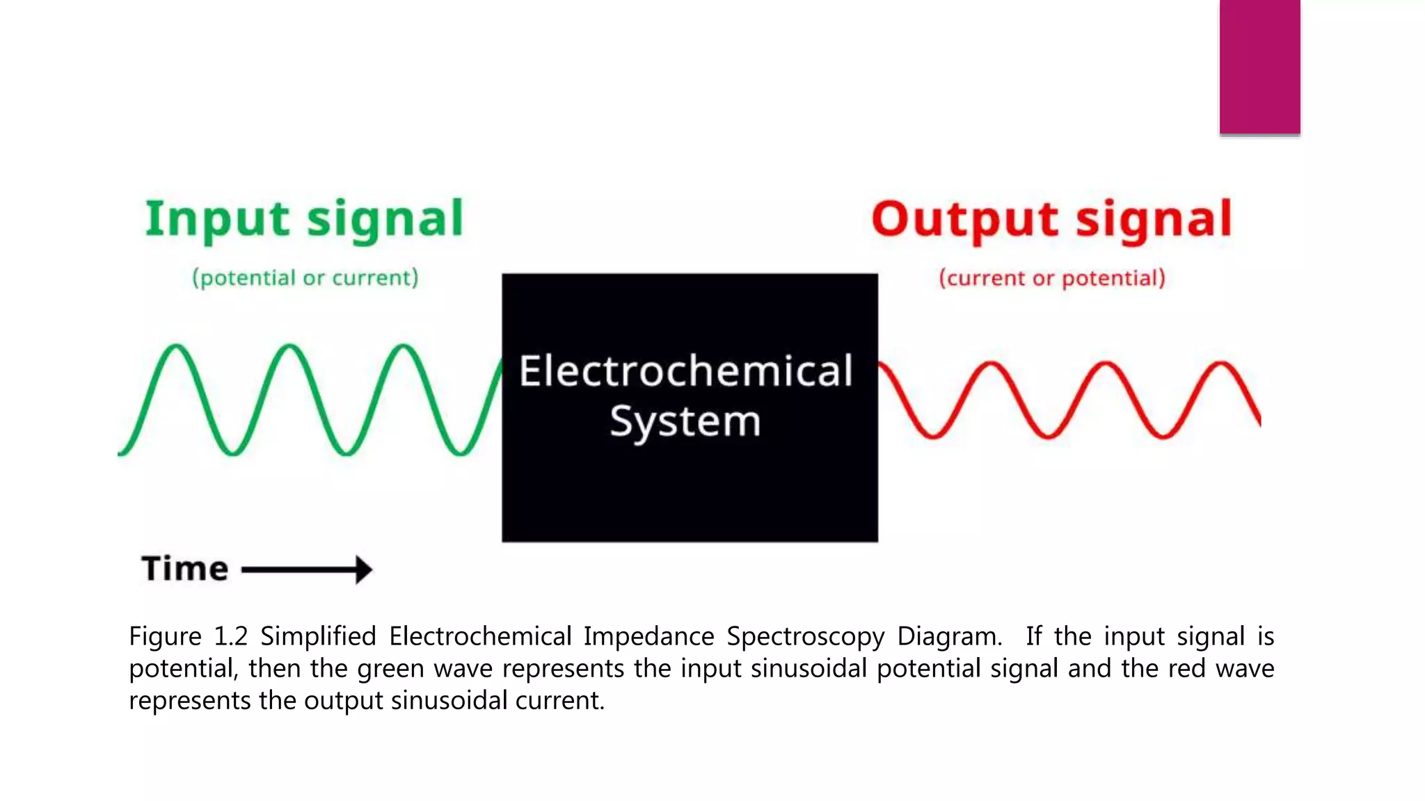
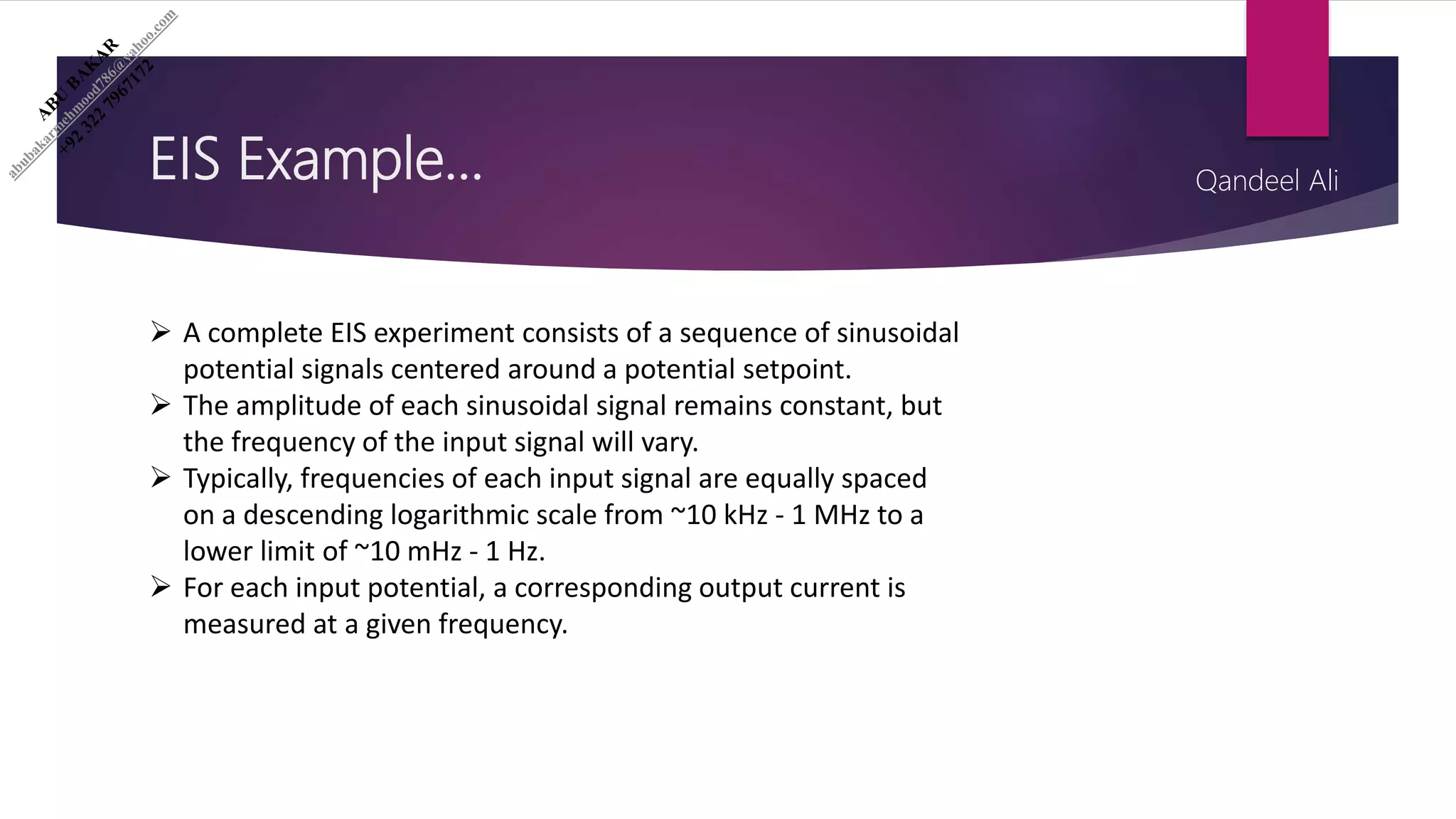
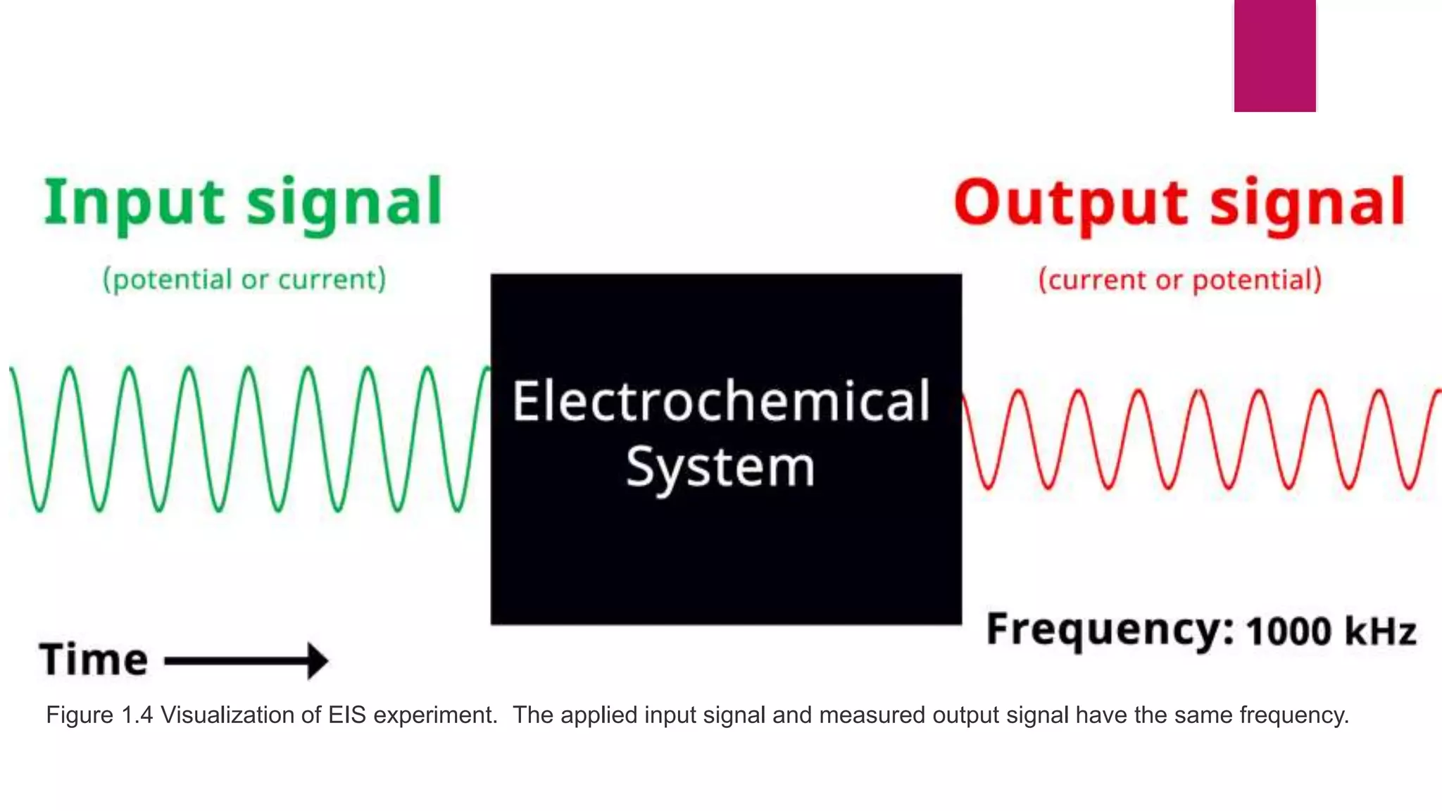
Electrochemical Impedance Spectroscopy (EIS) measures the impedance of a system under an alternating current at varying frequencies. Impedance is analogous to resistance in AC circuits, where the applied signal is sinusoidal rather than static. An EIS experiment applies a range of sinusoidal potential signals to a sample and measures the corresponding output currents. The impedance and phase shift between input and output are plotted versus frequency on Bode or Nyquist plots to characterize the system. EIS is used to study electrode kinetics and mass transport phenomena in electrochemical cells.

3. Electrochemical Impedance
Spectroscopy (EIS) Basics

4. Introduction
 Electrochemical Impedance Spectroscopy
(EIS) is a very complex subject in
electroanalytical chemistry.
 To understand electrochemical impedance
spectroscopy, we will start with the concept of
electrical resistance via Ohm's law.
𝑅 =
𝑉
𝐼
Syed Taha

5. 𝑅 =
𝑉(𝜔)
𝑖( )
 This description of resistance via Ohm's law applies
specifically to direct current (DC), where a static
voltage or current is applied across a resistor.
 Impedance, by contrast, is a measure of the
resistance a circuit experiences related to the
passage of an alternating electrical current (AC).
 In an AC system, the applied signal is no longer
static but oscillates as a sinusoidal wave at a given
frequency.
 The equation for impedance is analogous to Ohm's law;
however, instead of using for resistance we use for impedance
Continue….

6. Figure 1.2 Simplified Electrochemical Impedance Spectroscopy Diagram. If the input signal is
potential, then the green wave represents the input sinusoidal potential signal and the red wave
represents the output sinusoidal current.

7. E(t)= Eocos(𝜔𝑡)
Figure 1.3 Simplified Electrochemical Impedance Spectroscopy Diagram with Phase Angle. The teal
sinusoidal wave represents input potential signal visually overlapped in time with the output current
signal. Phase angle represents the shift in phase when the input and output signals are overlapped in
time.

8. EIS Example…
 A complete EIS experiment consists of a sequence of sinusoidal
potential signals centered around a potential setpoint.
 The amplitude of each sinusoidal signal remains constant, but
the frequency of the input signal will vary.
 Typically, frequencies of each input signal are equally spaced
on a descending logarithmic scale from ~10 kHz - 1 MHz to a
lower limit of ~10 mHz - 1 Hz.
 For each input potential, a corresponding output current is
measured at a given frequency.
Qandeel Ali

9. Figure 1.4 Visualization of EIS experiment. The applied input signal and measured output signal have the same frequency.

10. Figure 1.5 Lissajous plot where the input potential and output current are perfectly in phase. The resulting
curve is a straight line with a slope proportional to the impedance at that frequency.

11. Figure 1.6 Lissajous plot where the input potential and output current are out of phase. The resulting plot
is an oval.

12. EIS Instrumentation Zeeshan Haider

13. Basic Principle:-

14. Application of EIS:-

15. Bode plot Mian Ahmer
 In a bode plot, |Z| vs. frequency is displayed on the
primary vertical axis and ∅ 𝑣𝑠 𝑓 is displayed on the
secondary vertical axis.
 Frequency and impedance magnitude are normally
plotted on a logarithmic scale,while the phase angle
is displayed linearly.
 There is another way to express EIS data. Using polar
coordinates,let us plot |Z| as a ray originating from
the center at an angle equal to the phase angle
(Figure 2.3).
Figure 2.3 Plotting of Impedance Magnitude
and Phase Angle in Polar Coordinates

16. Continue…
If we move from polar to cartesian coordinates, we can break the
impedance magnitude into its x and y components (Figure 2.4).