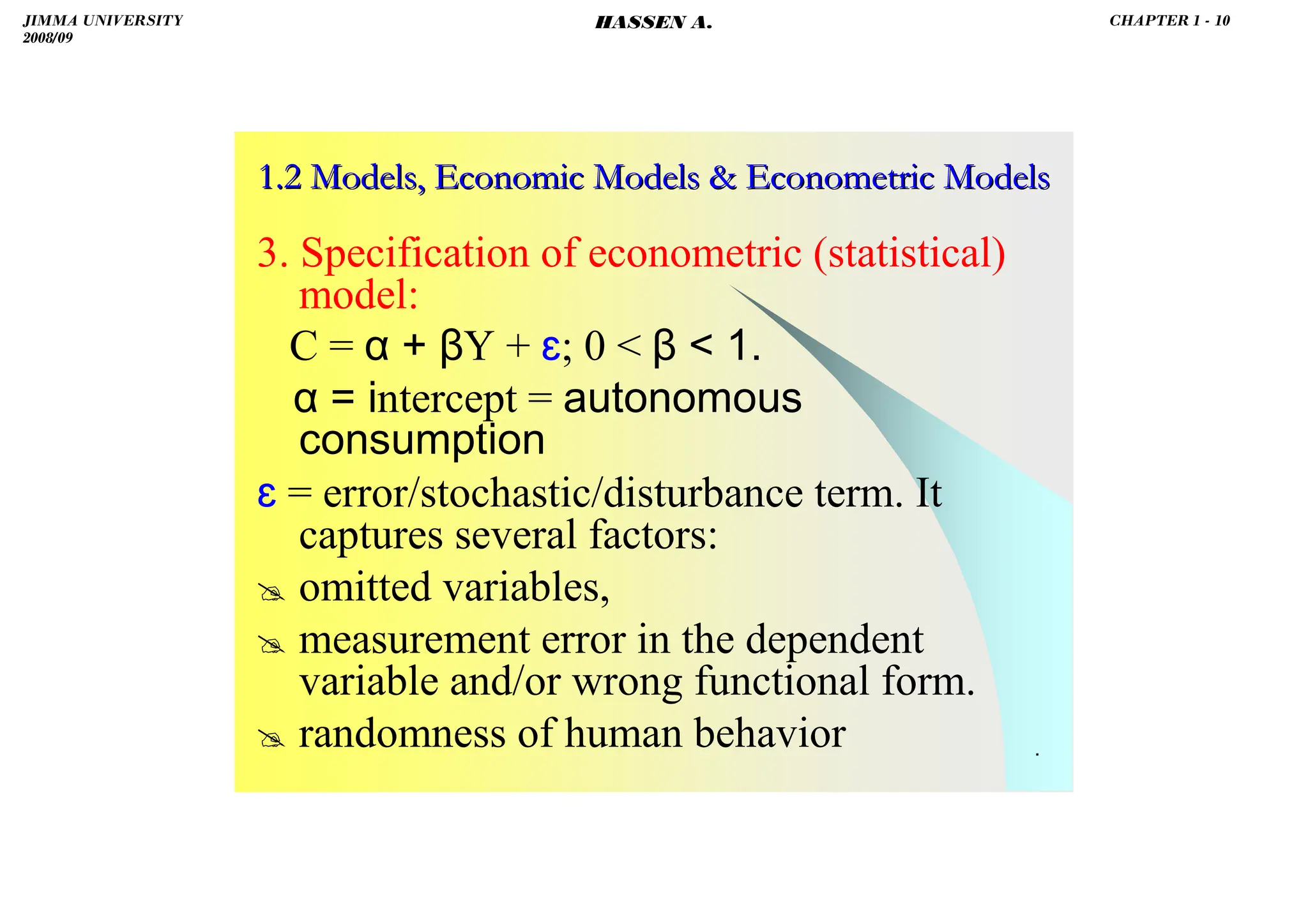
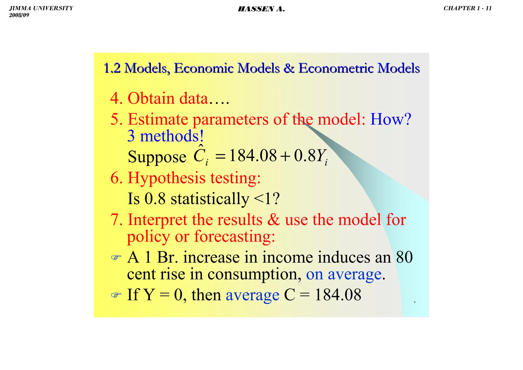
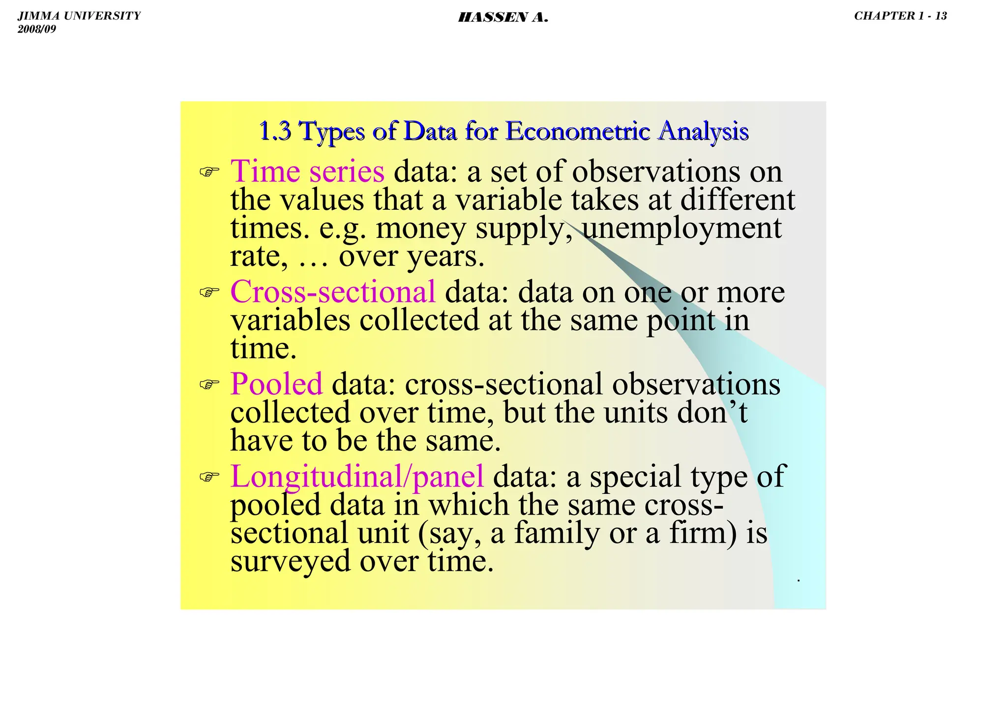
The document serves as an introduction to econometrics and its application in economic measurement through the use of statistical methods and theories. It covers key concepts such as econometric models, types of data, and regression analysis, emphasizing the importance of estimation, hypothesis testing, and policy evaluation. The text also highlights the method of least squares for fitting regression lines and the significance of understanding relationships between economic variables.

1. H
A
S
S
E
N
A
B
D
A .
INTRODUCTION TO
INTRODUCTION TO
ECONOMETRICS
ECONOMETRICS
(ECON. 352)
(ECON. 352)
HASSEN A. (M.Sc.)
HASSEN A. (M.Sc.)
JIMMA UNIVERSITY
2008/09
CHAPTER 1 - 1

2. HASSEN ABDA
.
CHAPTER ONE
INTRODUCTION
1.1 The Econometric Approach
1.2 Models, Economic Models &
Econometric Models
1.3 Types of Data for Econometric
Analysis
JIMMA UNIVERSITY
2008/09
CHAPTER 1 - 2
HASSEN A.

3. HASSEN ABDA
.
1.1 The Econometric Approach
1.1 The Econometric Approach
WHAT IS ECONOMETRICS?
Econometrics means “economic
measurement”
In simple terms, econometrics deals
with the application of statistical
methods to economics.
The application of mathematical
statistical techniques to data in order to
collect evidence on questions of interest
to economics.
JIMMA UNIVERSITY
2008/09
CHAPTER 1 - 3
HASSEN A.

4. HASSEN ABDA
.
1.1 The Econometric Approach
1.1 The Econometric Approach
Unlike economic statistics, which
mainly collects summarizes statistical
data, econometrics combines economic
theory, mathematical economics,
economic statistics mathematical
statistics:
economic theory: providing the
theory, or, imposing a logical
structure on the form of the
question). e.g., when price goes
up, quantity demanded goes down.
JIMMA UNIVERSITY
2008/09
CHAPTER 1 - 4
HASSEN A.

5. HASSEN ABDA
.
mathematical economics:
expressing economic theory
using math (mathematical form).
economic statistics: data
presentation description.
mathematical statistics:
estimation testing techniques.
1.1 The Econometric Approach
1.1 The Econometric Approach
JIMMA UNIVERSITY
2008/09
CHAPTER 1 - 5
HASSEN A.

6. HASSEN ABDA
.
1.1 The Econometric Approach
1.1 The Econometric Approach
Goals/uses of econometrics
Estimation/measurement of
economic parameters or
relationships, which may be needed
for policy- or decision-making;
Testing ( possibly refining)
economic theory;
Forecasting/prediction of future
values of economic magnitudes;
Evaluation of policies/programs.
JIMMA UNIVERSITY
2008/09
CHAPTER 1 - 6
HASSEN A.

7. HASSEN ABDA
.
1.2 Models, Economic Models Econometric Models
1.2 Models, Economic Models Econometric Models
Model: a simplified representation of
the real world phenomena.
Combines the economic model
with assumptions about the
random nature of the data
MODEL
ECONOMIC MODEL
ECONOMETRIC
MODEL
JIMMA UNIVERSITY
2008/09
CHAPTER 1 - 7
HASSEN A.

8. HASSEN ABDA
.
1. Economic theory or model
2. Econometric model: a
statement of the economic theory
in an empirically testable form
6. Tests of any hypothesis
suggested by the economic model
7. Interpreting results using the
model for prediction policy
5. Estimation of the model
3. Data
4. Some
priori
information
1.2 Models, Economic Models Econometric Models
1.2 Models, Economic Models Econometric Models
JIMMA UNIVERSITY
2008/09
CHAPTER 1 - 8
HASSEN A.

9. HASSEN ABDA
.
1.2 Models, Economic Models Econometric Models
1.2 Models, Economic Models Econometric Models
1. Statement of theory or hypothesis:
e.g. Theory: people increase
consumption as income increases, but
not by as much as the increase in their
income.
2. Specification of mathematical model:
C = α + βY; 0 β 1.
where: C = Consumption,
Y = Income,
β = slope = MPC = ∆C/∆Y,
α = intercept
JIMMA UNIVERSITY
2008/09
CHAPTER 1 - 9
HASSEN A.

10. HASSEN ABDA
.
1.2 Models, Economic Models Econometric Models
1.2 Models, Economic Models Econometric Models
3. Specification of econometric (statistical)
model:
C = α + βY + ɛ; 0 β 1.
α = intercept = autonomous
consumption
ɛ = error/stochastic/disturbance term. It
captures several factors:
omitted variables,
measurement error in the dependent
variable and/or wrong functional form.
randomness of human behavior
JIMMA UNIVERSITY
2008/09
CHAPTER 1 - 10
HASSEN A.

11. HASSEN ABDA
.
1.2 Models, Economic Models Econometric Models
1.2 Models, Economic Models Econometric Models
4. Obtain data….
5. Estimate parameters of the model: How?
3 methods!
Suppose
6. Hypothesis testing:
Is 0.8 statistically 1?
7. Interpret the results use the model for
policy or forecasting:
A 1 Br. increase in income induces an 80
cent rise in consumption, on average.
If Y = 0, then average C = 184.08
i
i Y
C 8
.
0
08
.
184
ˆ +
=
JIMMA UNIVERSITY
2008/09
CHAPTER 1 - 11
HASSEN A.

12. HASSEN ABDA
.
Predict the level of C for a given Y,
Pick the value of the control variable
(Y) to get a desired value of the target
variable (C), …
1.2 Models, Economic Models Econometric Models
1.2 Models, Economic Models Econometric Models
JIMMA UNIVERSITY
2008/09
CHAPTER 1 - 12
HASSEN A.

13. HASSEN ABDA
.
Time series data: a set of observations on
the values that a variable takes at different
times. e.g. money supply, unemployment
rate, … over years.
Cross-sectional data: data on one or more
variables collected at the same point in
time.
Pooled data: cross-sectional observations
collected over time, but the units don’t
have to be the same.
Longitudinal/panel data: a special type of
pooled data in which the same cross-
sectional unit (say, a family or a firm) is
surveyed over time.
1.3 Types of Data for Econometric Analysis
1.3 Types of Data for Econometric Analysis
JIMMA UNIVERSITY
2008/09
CHAPTER 1 - 13
HASSEN A.

14. HASSEN ABDA
CHAPTER TWO
SIMPLE LINEAR REGRESSION
2.1 The Concept of Regression Analysis
2.2 The Simple Linear Regression Model
2.3 The Method of Least Squares
2.4 Properties of Least-Squares Estimators and the
Gauss-Markov Theorem
2.5 Residuals and Goodness of Fit
2.6 Confidence Intervals and Hypothesis Testing in
Regression Analysis
2.7 Prediction with the Simple Linear Regression
JIMMA UNIVERSITY
2008/09
CHAPTER 2 - 1
HASSEN A.

15. HASSEN ABDA
2.1 The Concept of Regression Analysis
Origin of the word regression!
Our objective in regression analysis is to find out
how the average value of the dependent variable (or
the regressand) varies with the given values of the
explanatory variable (or the regressor/s).
Compare regression correlation! (dependence vs.
association).
The key concept underlying regression analysis is
the conditional expectation function (CEF), or
population regression function (PRF).
)
(
]
|
[ i
i X
f
X
Y
E =
JIMMA UNIVERSITY
2008/09
CHAPTER 2 - 2
HASSEN A.

16. HASSEN ABDA
2.1 The Concept of Regression Analysis
For empirical purposes, it is the stochastic PRF that
matters.
The stochastic disturbance term ɛi plays a critical
role in estimating the PRF.
The PRF is an idealized concept, since in practice
one rarely has access to the entire population.
Usually, one has just a sample of observations.
Hence, we use the stochastic sample regression
function (SRF) to estimate the PRF, i.e., we
use: to estimate .
i
i
i X
Y
E
Y ε
+
= ]
|
[
)
i
e
,
i
Y
f
i
Y ˆ
(
= )
i
e
,
i
X
Y
E
f
i
Y
]
|
[
(
=
)
f(X
Y i
i =
ˆ
JIMMA UNIVERSITY
2008/09
CHAPTER 2 - 3
HASSEN A.

17. HASSEN ABDA
.
2.2 The Simple Linear Regression Model
We assume linear PRFs, i.e., regressions that are
linear in parameters (α and β). They may or may not
be linear in variables (Y or X).
Simple because we have only one regressor (X).
Accordingly, we use:
.
,
ˆ
,
ˆ
ly
respective
,
and
of
estimates
re
sample
a
from
and
i
a
i
e
ε
β
α
β
α
⇒
.
i
i X
X
Y
E
estimate
to
i
X
i
Y β
α
β
α +
=
+
= ]
|
[
ˆ
ˆ
ˆ
i
i X
X
Y
E β
α+
=
]
|
[ i
i
i X
Y ε
β
α +
+
=
⇒
JIMMA UNIVERSITY
2008/09
CHAPTER 2 - 4
HASSEN A.

18. HASSEN ABDA
2.2 The Simple Linear Regression Model
Using the theoretical relationship between X and Y,
Yi can be decomposed into its non-stochastic
component α+βXi and its random component ɛi.
This is a theoretical decomposition because we do
not know the values of α and β, or the values of ɛ.
An operational decomposition of Y (used for
practical purposes) is with reference to the fitted
line. The actual value of Y is equal to the fitted
value plus the residual ei.
The residuals ei serve a similar purpose as the
stochastic term ɛi, but the two are not identical.
i
i X
Y β
α ˆ
ˆ
ˆ +
=
JIMMA UNIVERSITY
2008/09
CHAPTER 2 - 5
HASSEN A.

19. HASSEN ABDA
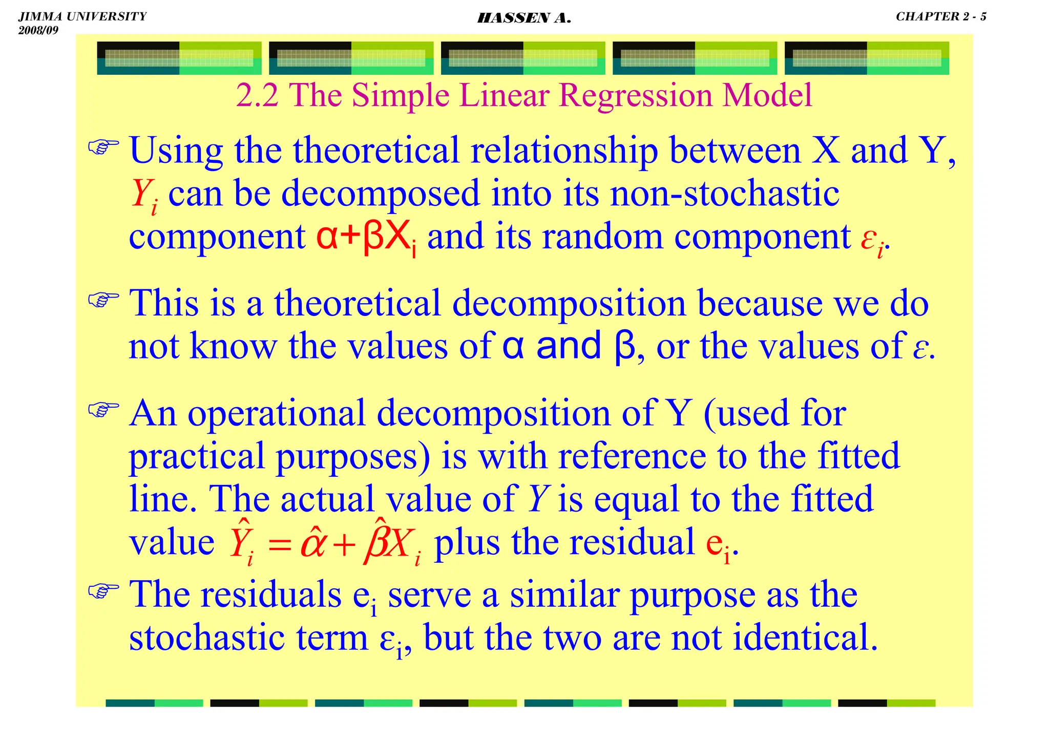
2.2 The Simple Linear Regression Model
From the PRF:
From the SRF:
i
i
i X
Y
E
Y i
ε
+
= ]
|
[
i
e
i
Y
i
Y +
= ˆ
]
|
[ i
i
i X
Y
E
Y i
−
=
ε
i
i
i X
X
Y
E
but β
α +
=
]
|
[
,
iiii
iiii
iiii
β
X
β
X
β
X
β
X
αααα
YYYY
εεεε
−
−
=
i
i
i Y
Y
e ˆ
−
=
i
X
Y
but i β
α ˆ
ˆ
ˆ +
=
iiii
XXXX
ββββ
αααα
YYYY
eeee
iiii
iiii
ˆ
ˆ −
−
=
JIMMA UNIVERSITY
2008/09
CHAPTER 2 - 6
HASSEN A.

20. HASSEN ABDA
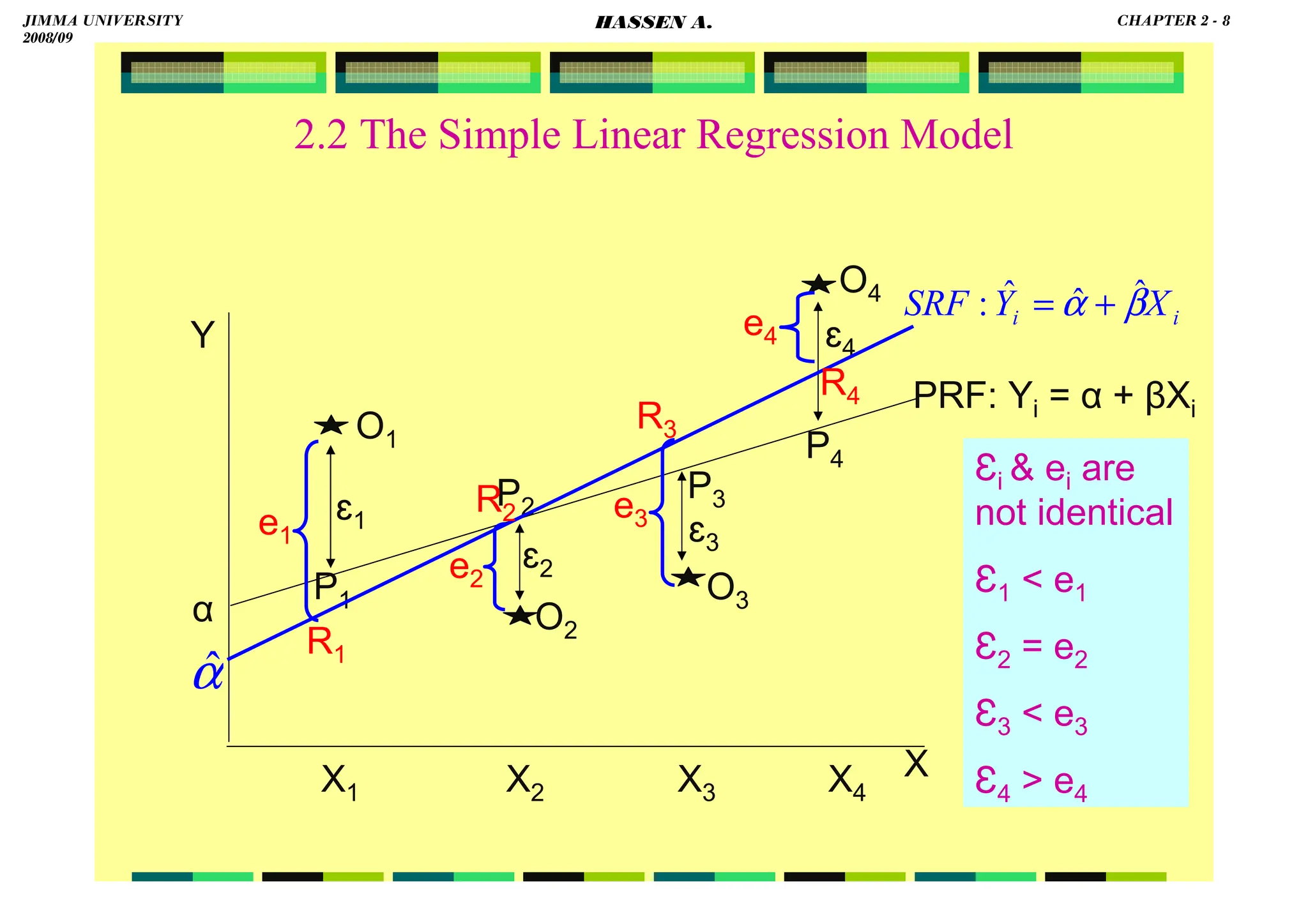
2.2 The Simple Linear Regression Model
O1 P4
α
X
P3
P2
O4
O3
O2
P1
E[Y|Xi] = α + βXi
Y
ɛ1
ɛ2
ɛ3
ɛ4
X1 X2 X3 X4
E[Y|X2] = α + βX2
JIMMA UNIVERSITY
2008/09
CHAPTER 2 - 7
HASSEN A.

21. HASSEN ABDA
2.2 The Simple Linear Regression Model
i
i X
Y
SRF β
α ˆ
ˆ
ˆ
: +
=
O1 P4
α
X
P3
P2
O4
O3
O2
P1
PRF: Yi = α + βXi
Y
ɛ1
ɛ2
ɛ3
ɛ4
e1
e2
e3
e4
α̂
R1
R2
R3
R4
Ɛi ei are
not identical
Ɛ1 e1
Ɛ2 = e2
Ɛ3 e3
Ɛ4 e4
X1 X2 X3 X4
JIMMA UNIVERSITY
2008/09
CHAPTER 2 - 8
HASSEN A.

22. HASSEN ABDA
2.3 The Method of Least Squares
Remember that our sample is only one of the large
number of possibilities.
Implication: the SRF line in the figure above is just
one of the many possible such lines. Each of the
SRF lines has unique values.
Then, which of these lines should we choose?
Generally we will look for the SRF which is very close
to the PRF.
But, how can we devise a rule that makes the SRF
as close as possible to the PRF? Equivalently, how
can we choose the best technique to estimate the
parameters of interest (α and β)?
β
α ˆ
ˆ and
JIMMA UNIVERSITY
2008/09
CHAPTER 2 - 9
HASSEN A.

23. HASSEN ABDA
Generally speaking, there are 3 methods of
estimation:
method of least squares,
method of moments, and
maximum likelihood estimation.
The most common method for fitting a regression
line is the method of least-squares. We will use
the LSE, specifically, the Ordinary Least Squares
(OLS) in Chapters 2 and 3.
What does the OLS do?
2.3 The Method of Least Squares
JIMMA UNIVERSITY
2008/09
CHAPTER 2 - 10
HASSEN A.

24. HASSEN ABDA
2.3 The Method of Least Squares
A line gives a good fit to a set of data if the points
(actual observations) are close to it. That is, the
predicted values obtained by using the line should
be close to the values that were actually observed.
Meaning, the residuals should be small. Therefore,
when assessing the fit of a line, the vertical distances
of the points to the line are the only distances that
matter because errors are measured as vertical
distances.
The OLS method calculates the best-fitting line for
the observed data by minimizing the sum of the
squares of the vertical deviations from each data
point to the line (the RSS).
JIMMA UNIVERSITY
2008/09
CHAPTER 2 - 11
HASSEN A.

25. HASSEN ABDA
2.3 The Method of Least Squares
Minimize RSS =
We could think of minimizing RSS by successively
choosing pairs of values for until RSS is
made as small as possible
But, we will use differential calculus (which turns
out to be a lot easier).
Why the squares of the residuals? Why not just
minimize the sum of the residuals?
To prevent negative residuals from cancelling
positive ones. Because the deviations are first
squared, then summed, there are no cancellations
between positive and negative values.
∑
=
n
i
i
e
1
2
β
α ˆ
ˆ and
JIMMA UNIVERSITY
2008/09
CHAPTER 2 - 12
HASSEN A.

26. HASSEN ABDA
2.3 The Method of Least Squares
If we use , all the error terms ei would receive
equal importance no matter how close or how
widely scattered the individual observations are
from the SRF.
A consequence of this is that it is quite possible that
the algebraic sum of the ei is small (even zero)
although the eis are widely scattered about the SRF.
Besides, the OLS estimates possess desirable
properties of estimators under some assumptions.
OLS Technique:
∑
=
n
i
i
e
1
∑ ∑ −
−
=
−
=
= =
=
∑
n
i
n
i
i
i
i
i
n
i
i )
X
β
α
(Y
)
Y
(Y
e
β
,
α
minimize 1 1
2
2
1
2 ˆ
ˆ
ˆ
ˆ
ˆ
JIMMA UNIVERSITY
2008/09
CHAPTER 2 - 13
HASSEN A.

27. HASSEN ABDA
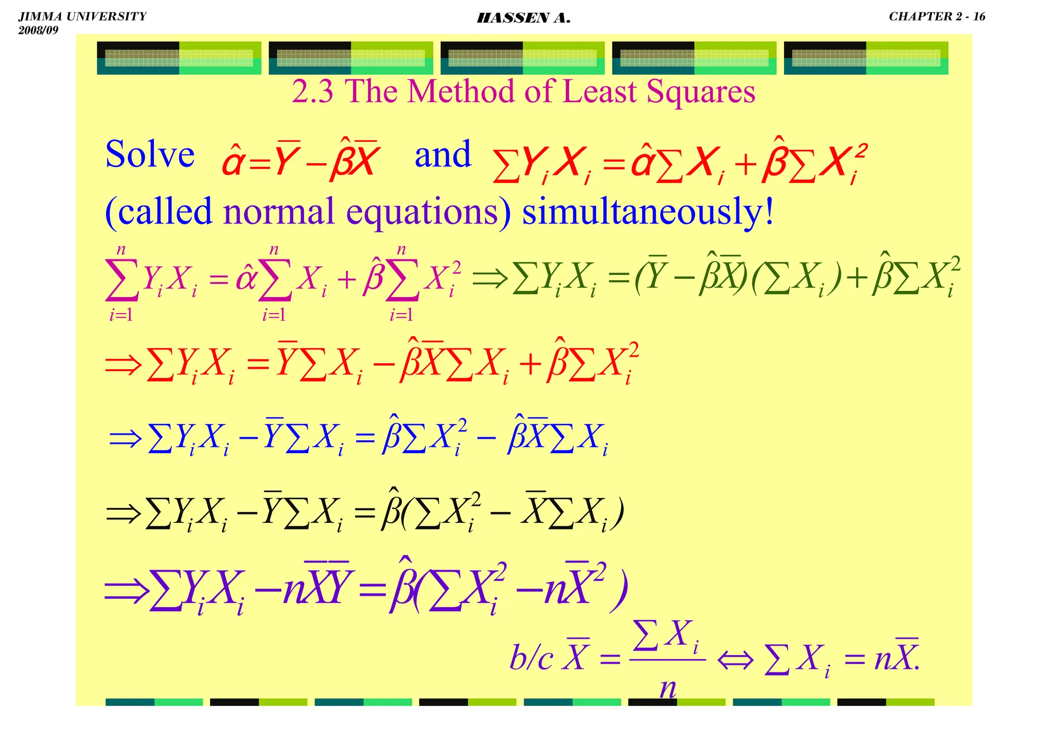
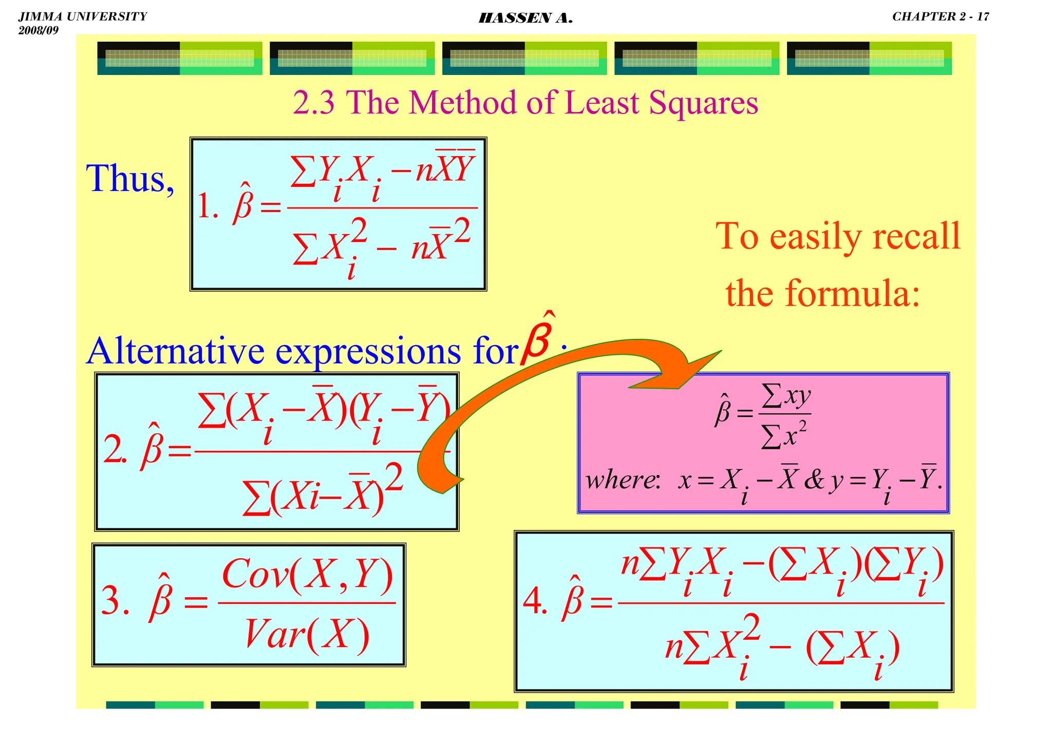
2.3 The Method of Least Squares
F.O.C.: (1)
0
ˆ
]
)
ˆ
ˆ
(
[
0
ˆ
)
(
1
2
1
2
=
∂
−
−
∂
⇒
=
∂
∂ ∑
∑ =
=
α
β
α
α
n
i
i
i
n
i
i X
Y
e
0
]
1
][
)
ˆ
ˆ
(
.[
2
1
=
−
−
−
⇒ ∑
=
n
i
i
i X
Y β
α
0
)
ˆ
ˆ
(
1
=
−
−
⇒ ∑
=
n
i
i
i X
Y β
α
0
ˆ
ˆ
1
1
1
=
−
−
⇒ ∑
∑
∑ =
=
=
n
i
i
n
i
n
i
i X
Y β
α
0
ˆ
ˆ =
−
−
⇒ X
Y β
α
XXXX
ββββ
YYYY
αααα
ˆ
ˆ −
=
⇒
.
0
ˆ
ˆ
1
1
=
−
−
⇒ ∑
∑ =
=
n
i
i
n
i
i X
n
Y β
α
JIMMA UNIVERSITY
2008/09
CHAPTER 2 - 14
HASSEN A.

28. HASSEN ABDA
2.3 The Method of Least Squares
F.O.C.: (2)
0
ˆ
]
)
ˆ
ˆ
(
[
0
ˆ
)
(
1
2
1
2
=
∂
−
−
∂
⇒
=
∂
∂ ∑
∑ =
=
β
β
α
β
n
i
i
i
n
i
i X
Y
e
0
]
][
)
ˆ
ˆ
(
.[
2
1
=
−
−
−
⇒ ∑
=
i
n
i
i
i X
X
Y β
α
0
)]
(
)
ˆ
ˆ
[(
1
=
−
−
⇒ ∑
=
i
n
i
i
i X
X
Y β
α
0
ˆ
ˆ
1
2
1
1
=
−
−
⇒ ∑
∑
∑ =
=
=
n
i
i
n
i
i
i
n
i
i X
X
X
Y β
α
∑
∑
∑ =
=
=
+
=
⇒
n
i
i
n
i
i
i
n
i
i X
X
X
Y
1
2
1
1
ˆ
ˆ β
α
JIMMA UNIVERSITY
2008/09
CHAPTER 2 - 15
HASSEN A.

29. HASSEN ABDA
2.3 The Method of Least Squares
Solve and
(called normal equations) simultaneously!
∑
+
∑
=
∑
2222
iiii
iiii
iiii
iiii
XXXX
ββββ
XXXX
αααα
XXXX
YYYY
ˆ
ˆ
∑
∑
∑ =
=
=
+
=
n
i
i
n
i
i
i
n
i
i X
X
X
Y
1
2
1
1
ˆ
ˆ β
α
XXXX
ββββ
YYYY
αααα
ˆ
ˆ −
=
∑
+
∑
−
=
∑
⇒ 2
ˆ
ˆ
i
i
i
i X
β
)
X
)(
X
β
Y
(
X
Y
∑
+
∑
−
∑
=
∑
⇒ 2
ˆ
ˆ
i
i
i
i
i X
β
X
X
β
X
Y
X
Y
∑
−
∑
=
∑
−
∑
⇒ i
i
i
i
i X
X
β
X
β
X
Y
X
Y ˆ
ˆ 2
)
X
X
X
(
β
X
Y
X
Y i
i
i
i
i ∑
−
∑
=
∑
−
∑
⇒ 2
ˆ
)
X
n
X
(
β
Y
X
n
X
Y 2
2
i
i
i −
∑
=
−
∑
⇒ ˆ
.
X
n
X
n
X
X
b/c i
i
=
∑
⇔
∑
=
JIMMA UNIVERSITY
2008/09
CHAPTER 2 - 16
HASSEN A.

30. HASSEN ABDA
17
2.3 The Method of Least Squares
Thus,
To easily recall
the formula:
Alternative expressions for :
ββββ
ˆ
2
2
ˆ
.
1
X
n
i
X
Y
X
n
i
X
i
Y
β
−
∑
−
∑
=
)
(
2
)
)(
(
ˆ
.
4
∑
−
∑
∑
∑
−
∑
=
i
X
i
X
n
i
Y
i
X
i
X
i
Y
n
β
∑ −
∑ −
−
=
2
)
(
)
)(
(
ˆ
.
2
X
Xi
Y
i
Y
X
i
X
β
)
(
)
,
(
ˆ
.
3
X
Var
Y
X
Cov
β =
.
:
ˆ
2
Y
i
Y
y
X
i
X
x
where
x
xy
β
−
=
−
=
∑
∑
=
JIMMA UNIVERSITY
2008/09
CHAPTER 2 - 17
HASSEN A.

31. HASSEN ABDA
18
2.3 The Method of Least Squares
for just use:
Or, if you wish:
XXXX
ββββ
YYYY
αααα
ˆ
ˆ −
=
]}
2
X
n
2
i
X
Y
X
n
i
X
i
Y
.[
X
{
Y
α
−
∑
−
∑
−
=
ˆ
2
X
n
2
i
X
i
X
i
Y
X
2
i
X
Y
α
−
∑
∑
−
∑
=
⇒ ˆ
2
X
n
2
i
X
]
Y
2
X
n
i
X
i
Y
X
Y
]
2
X
n
2
i
X
α
−
∑
−
∑
−
−
∑
=
⇒
[
[
ˆ
2
X
n
2
i
X
Y
2
X
n
i
X
i
Y
X
Y
2
X
n
2
i
X
Y
α
−
∑
+
∑
−
−
∑
=
⇒ ˆ
)
(
)
)(
(
)
)(
(
ˆ
2
X
n
2
i
X
n
i
X
i
Y
i
X
2
i
X
i
Y
α
−
∑
∑
∑
−
∑
∑
=
⇒
αααα
ˆ
JIMMA UNIVERSITY
2008/09
CHAPTER 2 - 18
HASSEN A.

32. HASSEN ABDA
19
2.3 The Method of Least Squares
Previously, we came across the following two
normal equations:
this is equivalent to:
equivalently,
Note also the following property:
0
)]
(
)
ˆ
ˆ
[(
1
=
−
−
∑
=
i
n
i
i
i X
X
Y
2. β
α
0
)
ˆ
ˆ
(
.
1
1
=
−
−
∑
=
n
i
i
i X
Y β
α 0
1
=
∑
=
n
i
i
e
0
1
=
∑
=
n
i
i
i X
e
i
e
i
Y
i
Y +
= ˆ
Y
Y ˆ
=
n
i
e
n
i
Y
n
i
Y ∑
∑
∑
+
=
⇒
ˆ
∑
∑
∑ +
=
⇒
i
e
i
Y
i
Y ˆ
.
0
0
ˆ =
⇔
=
=
⇒ ∑ e
i
e
since
Y
Y
JIMMA UNIVERSITY
2008/09
CHAPTER 2 - 19
HASSEN A.

33. HASSEN ABDA
2.3 The Method of Least Squares
The facts that and have the same average and
that this average value is achieved at the average
value of X (i.e., ) together imply
that the sample regression line passes through the
sample mean/average values of X and Y.
Ŷ Y
Y
Y ˆ
=
i
i X
Y β
α ˆ
ˆ
ˆ +
=
X
Y
Y
X
X
Y β
α ˆ
ˆ +
=
JIMMA UNIVERSITY
2008/09
CHAPTER 2 - 20
HASSEN A.

34. HASSEN ABDA
2.3 The Method of Least Squares
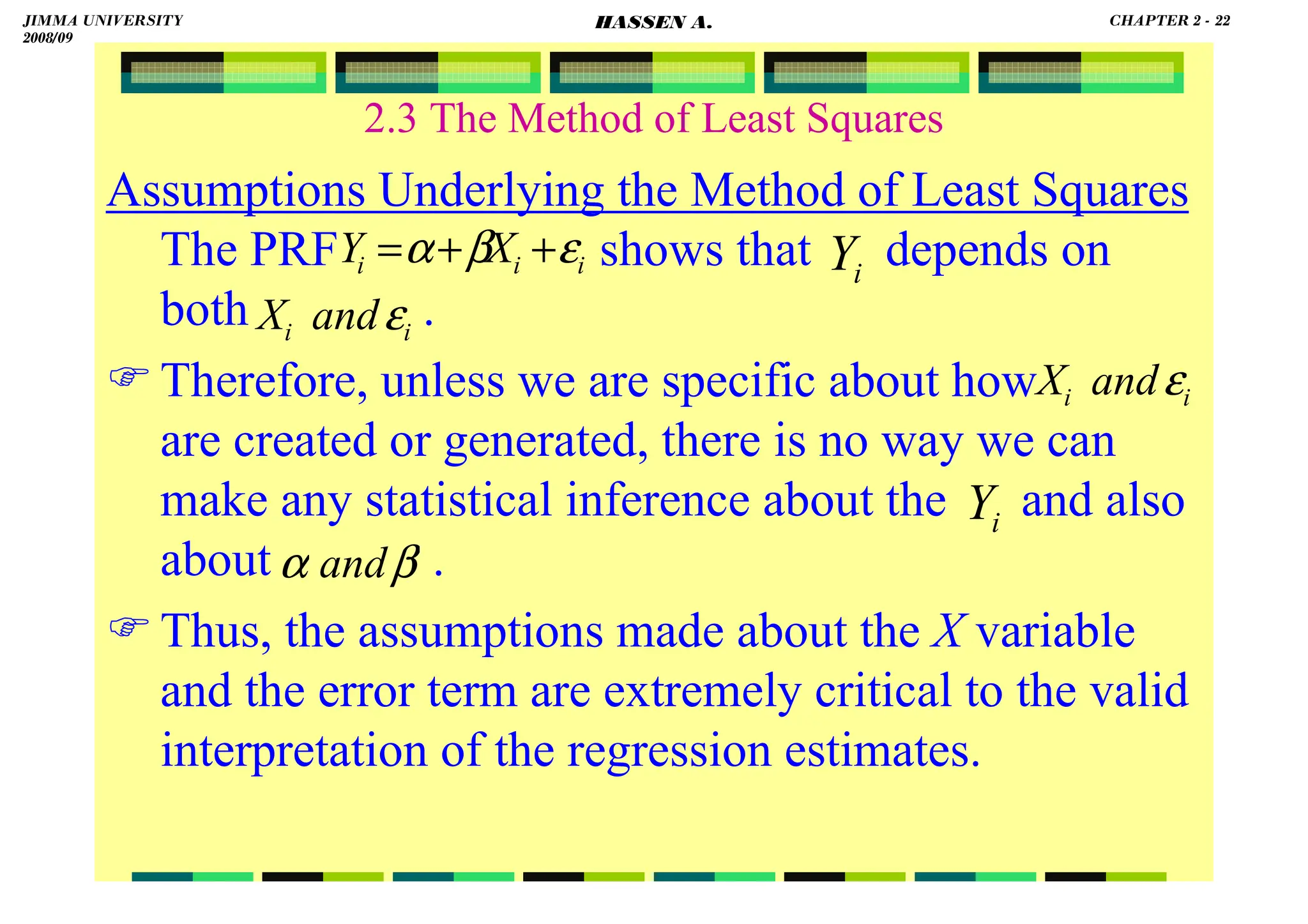
Assumptions Underlying the Method of Least Squares
To obtain the estimates of α and β, assuming that
our model is correctly specified and that the
systematic and the stochastic components in the
equation are independent suffice.
But the objective in regression analysis is not only
to obtain but also to draw inferences about
the true . For example, we’d like to know
how close are to or to .
To that end, we must not only specify the functional
form of the model, but also make certain assumps
about the manner in which are generated.
i
Y
]
|
[ i
X
Y
E
i
Ŷ
β
α ˆ
ˆ and
β
α ˆ
ˆ and
β
α and
β
α and
JIMMA UNIVERSITY
2008/09
CHAPTER 2 - 21
HASSEN A.

35. HASSEN ABDA
2.3 The Method of Least Squares
Assumptions Underlying the Method of Least Squares
The PRF shows that depends on
both .
Therefore, unless we are specific about how
are created or generated, there is no way we can
make any statistical inference about the and also
about .
Thus, the assumptions made about the X variable
and the error term are extremely critical to the valid
interpretation of the regression estimates.
i
Y
i
Y
β
α and
i
i
i X
Y ε
β
α +
+
=
i
i and
X ε
i
i and
X ε
JIMMA UNIVERSITY
2008/09
CHAPTER 2 - 22
HASSEN A.

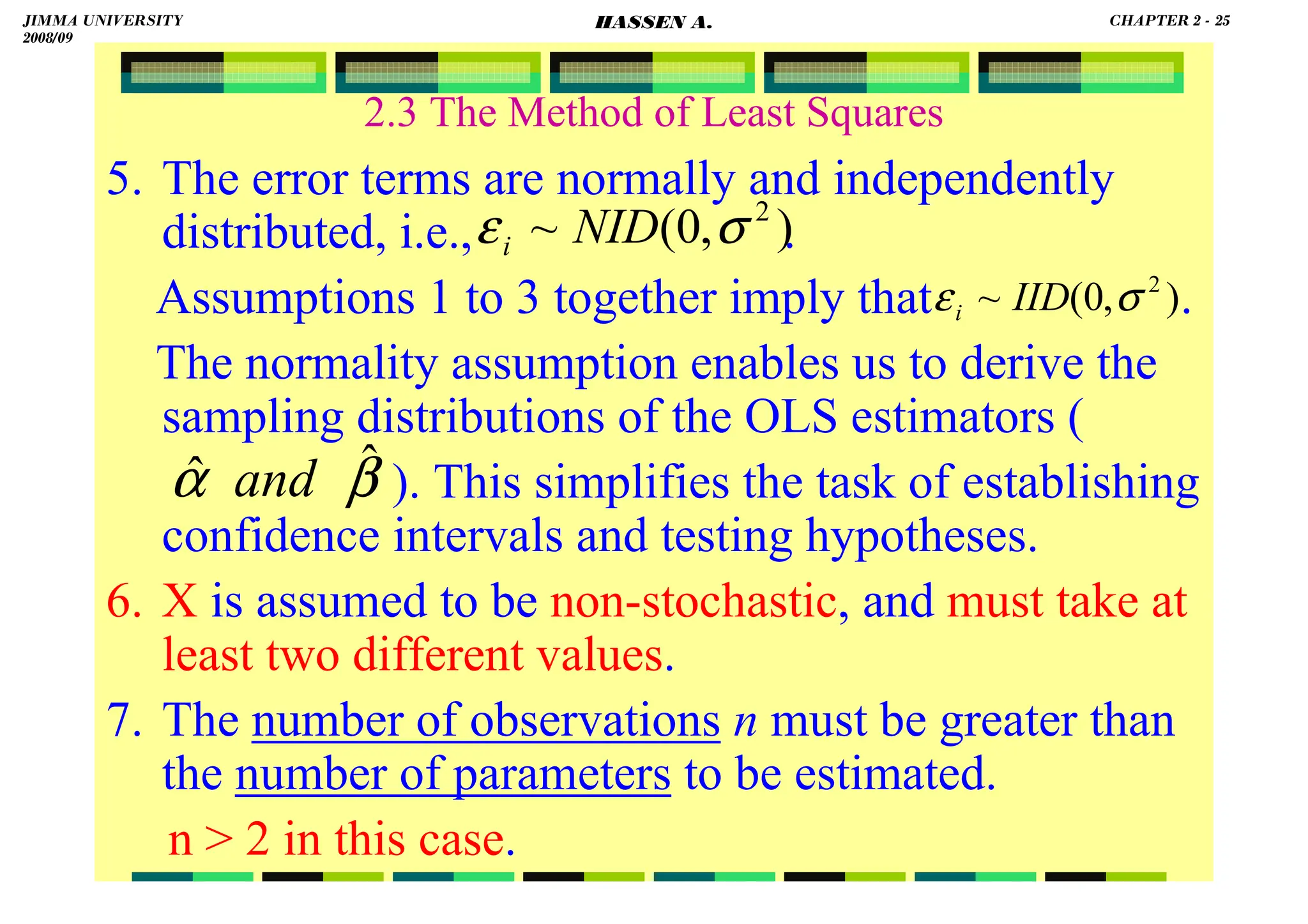
36. HASSEN ABDA
2.3 The Method of Least Squares
THE ASSUMPTIONS:
1. Zero mean value of disturbance, ɛi: E(ɛi|Xi) = 0.
Or equivalently, E[Yi|Xi] = α + βXi.
2. Homoscedasticity or equal variance of ɛi. Given the
value of X, the variance of ɛi is the same (finite
positive constant σ2) for all observations. That is,
var(ɛi|Xi) = E[ɛi–E(ɛi|Xi)]2 = E(ɛi)2 = σ2.
By implication: var(Yi|Xi) = σ2.
var(Yi|Xi) = E{α+βXi+ɛi – (α+βXi)}2
= E(ɛi)2
= σ2 for all i.
JIMMA UNIVERSITY
2008/09
CHAPTER 2 - 23
HASSEN A.

37. HASSEN ABDA
2.3 The Method of Least Squares
3. No autocorrelation between the disturbance terms.
Each random error term ɛi has zero covariance
with, or is uncorrelated with, each and every other
random error term ɛs (for s ≠ i).
cov(ɛi,ɛs|Xi,Xs) = E{[ɛi−E(ɛi)]|Xi}{[ɛs−E(ɛs)]|Xs} =
E(ɛi|Xi)(ɛs|Xs) = 0.
Equivalently, cov(Yi,Ys|Xi,Xs) = 0. (for all s ≠ i).
4. The disturbance ɛ and explanatory variable X are
uncorrelated. cov(ɛi,Xi) = 0.
cov(ɛi,Xi) = E[ɛi−E(ɛi)][Xi−E(Xi)]
= E[ɛi(Xi−E(Xi))]
= E(ɛiXi)−E(Xi)E(ɛi) = E(ɛiXi) = 0
JIMMA UNIVERSITY
2008/09
CHAPTER 2 - 24
HASSEN A.

38. HASSEN ABDA
2.3 The Method of Least Squares
5. The error terms are normally and independently
distributed, i.e., .
Assumptions 1 to 3 together imply that .
The normality assumption enables us to derive the
sampling distributions of the OLS estimators (
). This simplifies the task of establishing
confidence intervals and testing hypotheses.
6. X is assumed to be non-stochastic, and must take at
least two different values.
7. The number of observations n must be greater than
the number of parameters to be estimated.
n 2 in this case.
)
,
0
(
~ 2
σ
ε NID
i
β
α ˆ
ˆ and
)
,
0
(
~ 2
σ
ε IID
i
JIMMA UNIVERSITY
2008/09
CHAPTER 2 - 25
HASSEN A.

39. HASSEN ABDA
2.3 The Method of Least Squares
Numerical
Example:
Explaining sales
= f(advertising)
Sales are in
thousands
of Birr
advertising
expenses are in
hundreds of Birr.
10
11
10
9
7
10
6
12
10
11
Sales (Yi)
10
10
9
9
7
8
6
7
8
6
8
5
5
4
10
3
7
2
10
1
Advertising Expense (Xi)
Firm (i)
JIMMA UNIVERSITY
2008/09
CHAPTER 2 - 26
HASSEN A.

40. HASSEN ABDA
2.3 The Method of Least Squares
.
10
10
10
80
9
7
6
8
8
5
10
7
10
Xi
96
11
10
9
7
10
6
12
10
11
Yi
Ʃ
9
8
7
6
5
4
3
2
1
i
6
.
9
10
96
10
1
=
=
=
∑
=
n
Y
Y i
i
8
10
80
10
1
=
=
=
∑
=
n
X
X i
i
X
X
x i
i −
= i
i y
x
0.4
0
-1.4
-0.4
-0.6
-2.6
0.4
-3.6
2.4
0.4
1.4
Y
Y
y i
i −
=
0
2
1
-1
-2
0
0
-3
2
-1
2
0.8
21
1.4
-0.4
1.2
0
0
10.8
4.8
-0.4
2.8
JIMMA UNIVERSITY
2008/09
CHAPTER 2 - 27
HASSEN A.

41. HASSEN ABDA
2.3 The Method of Least Squares
.
28
4
1
1
4
0
0
9
4
1
4
2
0.16
0.4
10
30.4
1.96
0.16
0.36
6.76
1.96
12.96
5.76
0.16
1.96
0
1
-1
-2
0
0
-3
2
-1
2
0
-1.4
-0.4
-0.6
-2.6
0.4
-3.6
2.4
0.4
1.4
Ʃ
9
8
7
6
5
4
3
2
1
i
75
.
0
28
21
ˆ
2
=
=
=
∑
∑
i
i
i
x
y
x
β
i
y
6
.
3
)
8
(
75
.
0
6
.
9
ˆ
ˆ
=
−
=
−
= X
Y β
α
i
x
2
i
y 2
i
x
JIMMA UNIVERSITY
2008/09
CHAPTER 2 - 28
HASSEN A.

42. HASSEN ABDA
2.3 The Method of Least Squares
.
11.10
10
96
10.35
8.85
8.10
9.60
9.60
7.35
11.10
8.85
11.1
Ʃ
9
8
7
6
5
4
3
2
1
i
i
i X
Y 75
.
0
6
.
3
ˆ +
=
2
i
e
1.21
-1.10
0
0.65
1.15
0.90
-2.60
0.40
-1.35
0.90
1.15
-0.10
14.65
0.4225
1.3225
0.81
6.76
0.16
1.8225
0.81
1.3225
0.01
i
i
i Y
Y
e ˆ
−
=
65
.
14
2
=
∑ i
e
75
.
15
ˆ2
=
∑ i
y
4
.
30
2
=
∑ i
y
0
ˆ
=
=
=
=
∑
∑
∑
∑
i
i
i
i
e
y
x
y
JIMMA UNIVERSITY
2008/09
CHAPTER 2 - 29
HASSEN A.

43. HASSEN ABDA
2.4 Properties of OLS Estimators and the Gauss-Markov Theorem
☞Given the assumptions of the classical linear
regression model, the least-squares estimators
possess some ideal or optimum properties.
These statistical properties are extremely important
because they provide criteria for choosing among
alternative estimators.
These properties are contained in the well-known
Gauss–Markov Theorem.
JIMMA UNIVERSITY
2008/09
CHAPTER 2 - 30
HASSEN A.

44. HASSEN ABDA
2.4 Properties of OLS Estimators and the Gauss-Markov Theorem
Gauss-Markov Theorem: Under the above
assumptions of the linear regression model, the
estimators have the smallest variance of
all linear and unbiased estimators of . That
is, OLS estimators are the Best Linear Unbiased
Estimators (BLUE) of .
The Gauss-Markov Theorem does not depend on the
assumption of normality (of the error terms).
Let us prove that is the BLUE of !
β
α ˆ
ˆ and
β
α and
β
α and
β̂ β
JIMMA UNIVERSITY
2008/09
CHAPTER 2 - 31
HASSEN A.

45. HASSEN ABDA
2.4 Properties of OLS Estimators and the Gauss-Markov Theorem
Linearity of : (in a stochastic variable, ).
)
0
(sin
ˆ
2
2
2
=
=
−
=
∑
∑
∑
∑
∑
∑
∑
i
i
i
i
i
i
i
i
i
x
ce
x
Y
x
x
x
Y
x
Y
x
β
i
i
i
Y
x
x
∑
∑
=
⇒ )
(
ˆ
2
β
∑
∑ =
=
⇒ 2
ˆ
i
i
i
i
i
x
x
k
where
Y
k
β
n
nY
k
Y
k
Y
k +
+
+
=
⇒ ...
ˆ
2
2
1
1
β
∑
∑
∑
∑
∑
∑
∑
∑
−
=
−
=
=
2
2
2
2
)
(
ˆ
i
i
i
i
i
i
i
i
i
i
i
x
Y
x
x
Y
x
x
Y
Y
x
x
y
x
β
β̂ i
i or
Y ε
JIMMA UNIVERSITY
2008/09
CHAPTER 2 - 32
HASSEN A.

46. HASSEN ABDA
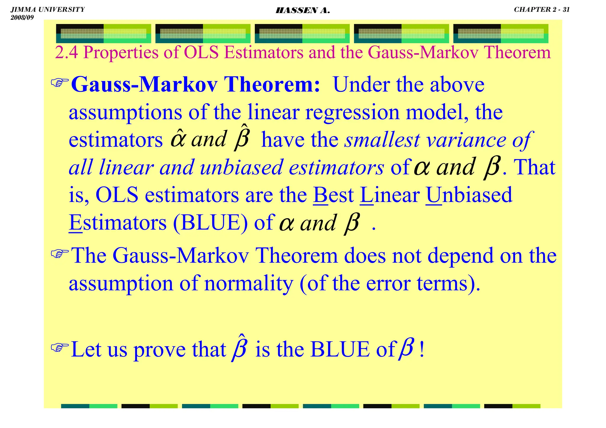
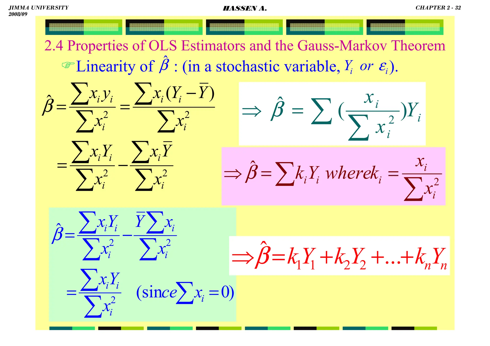
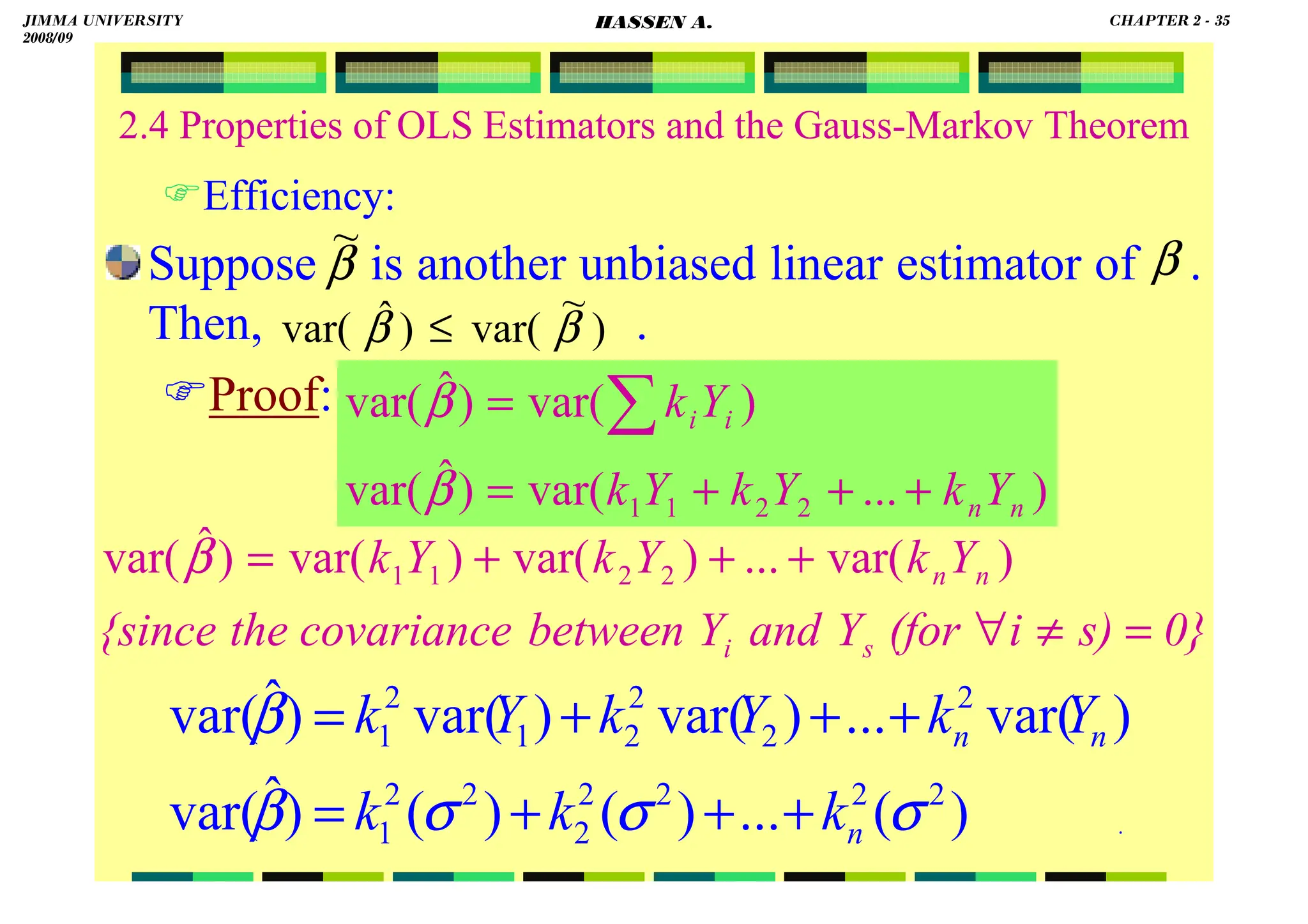
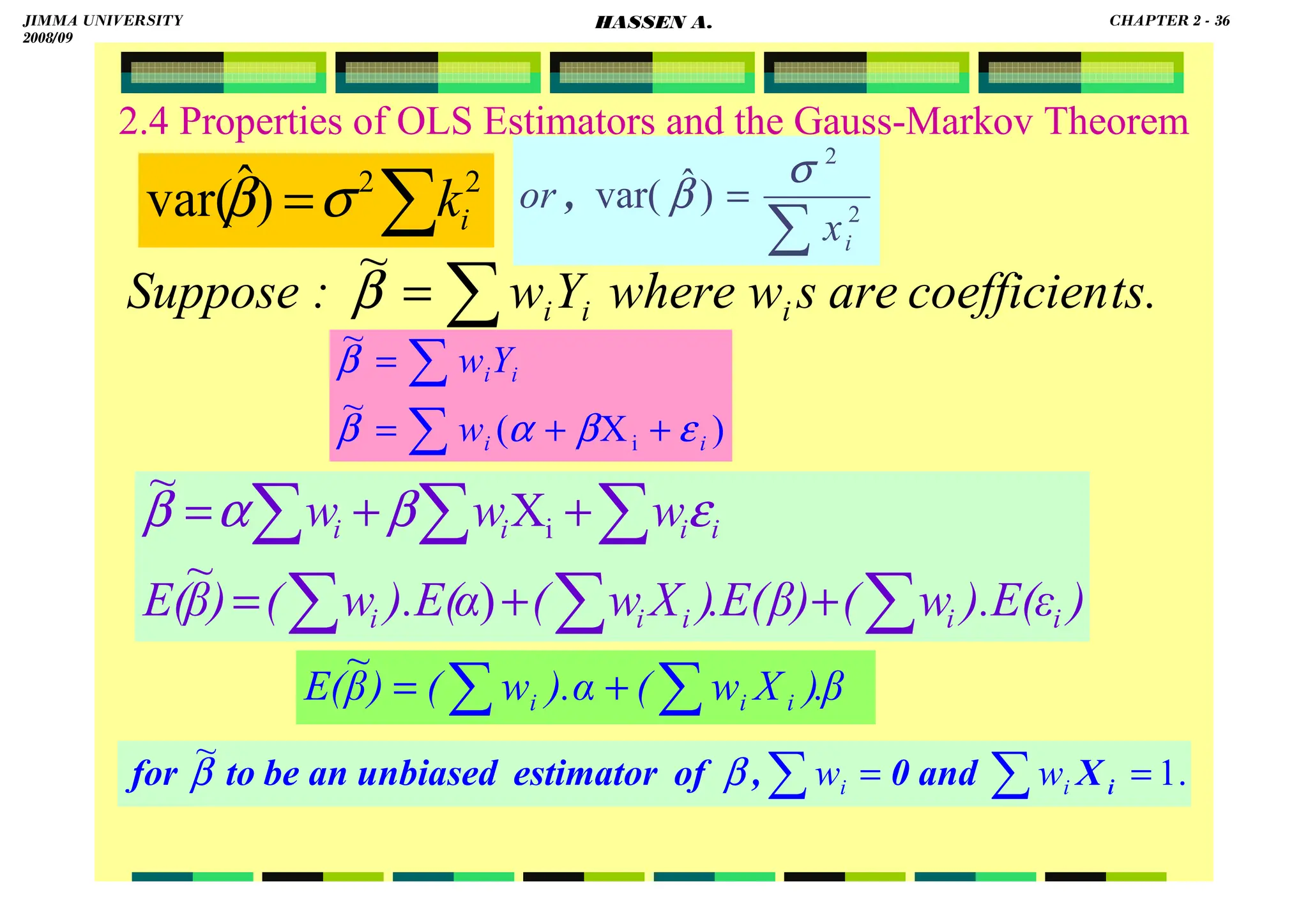
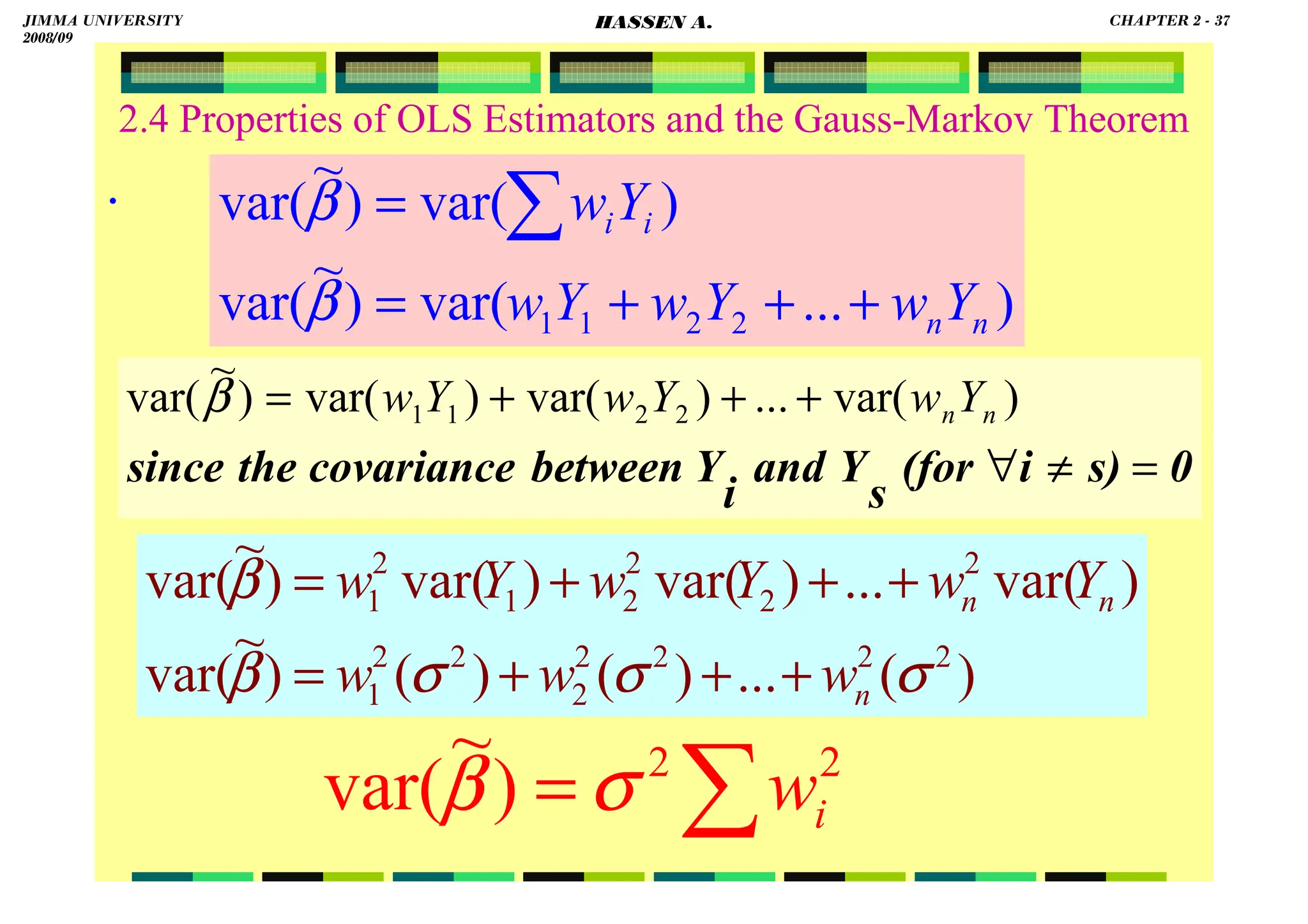
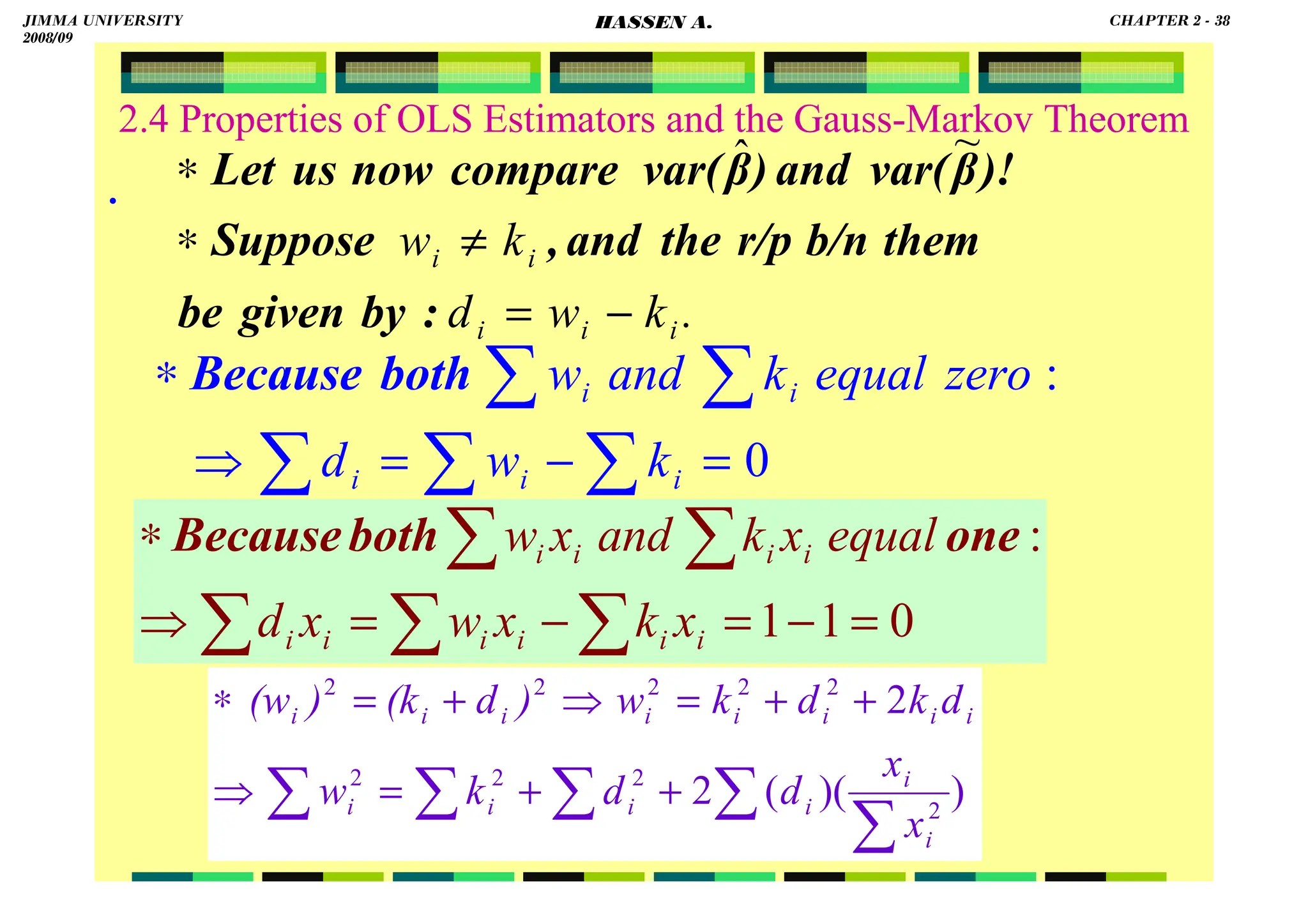
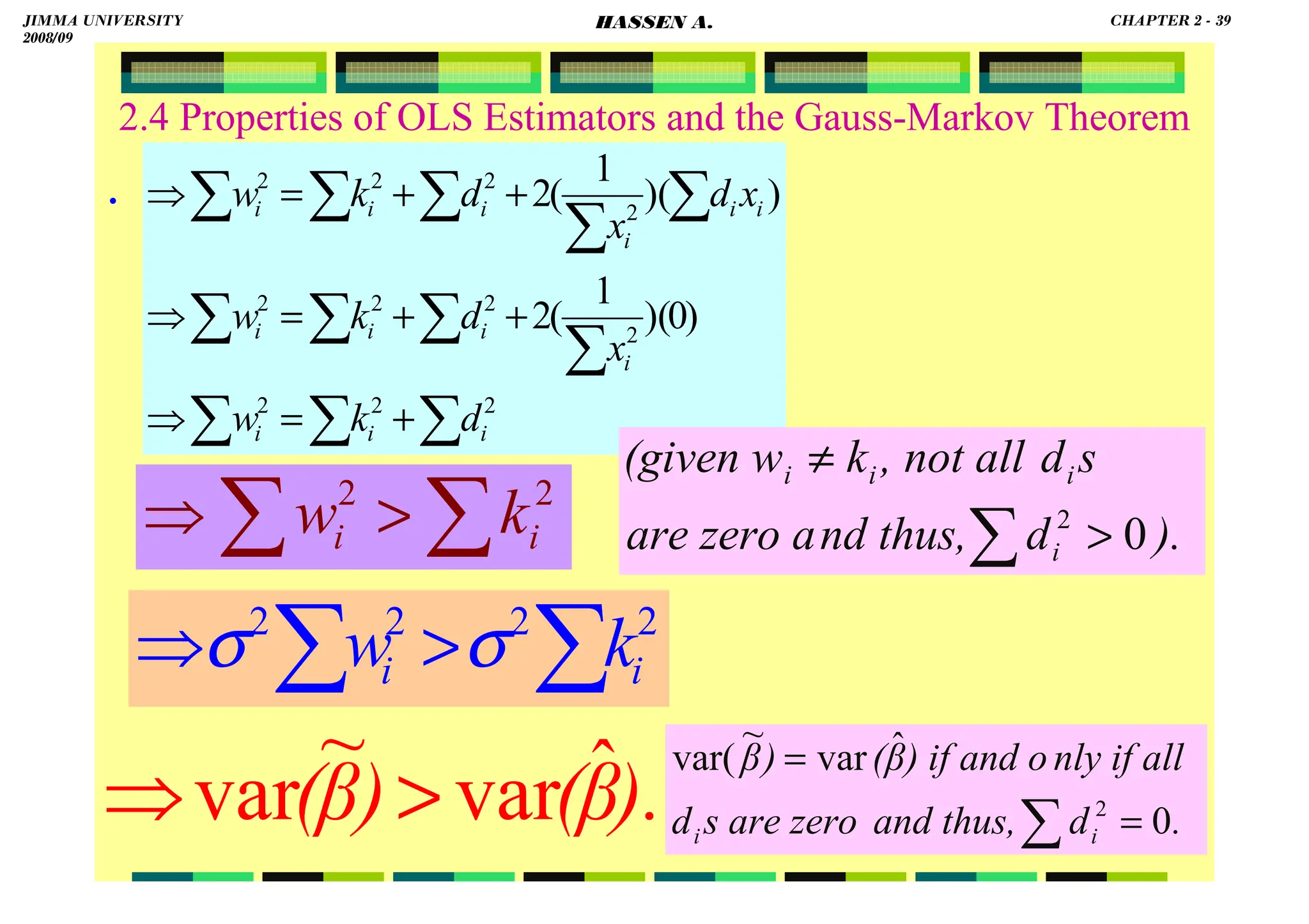
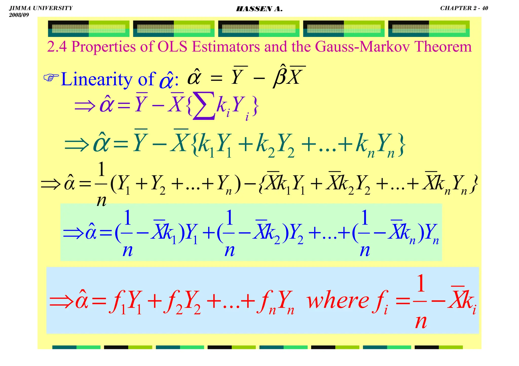
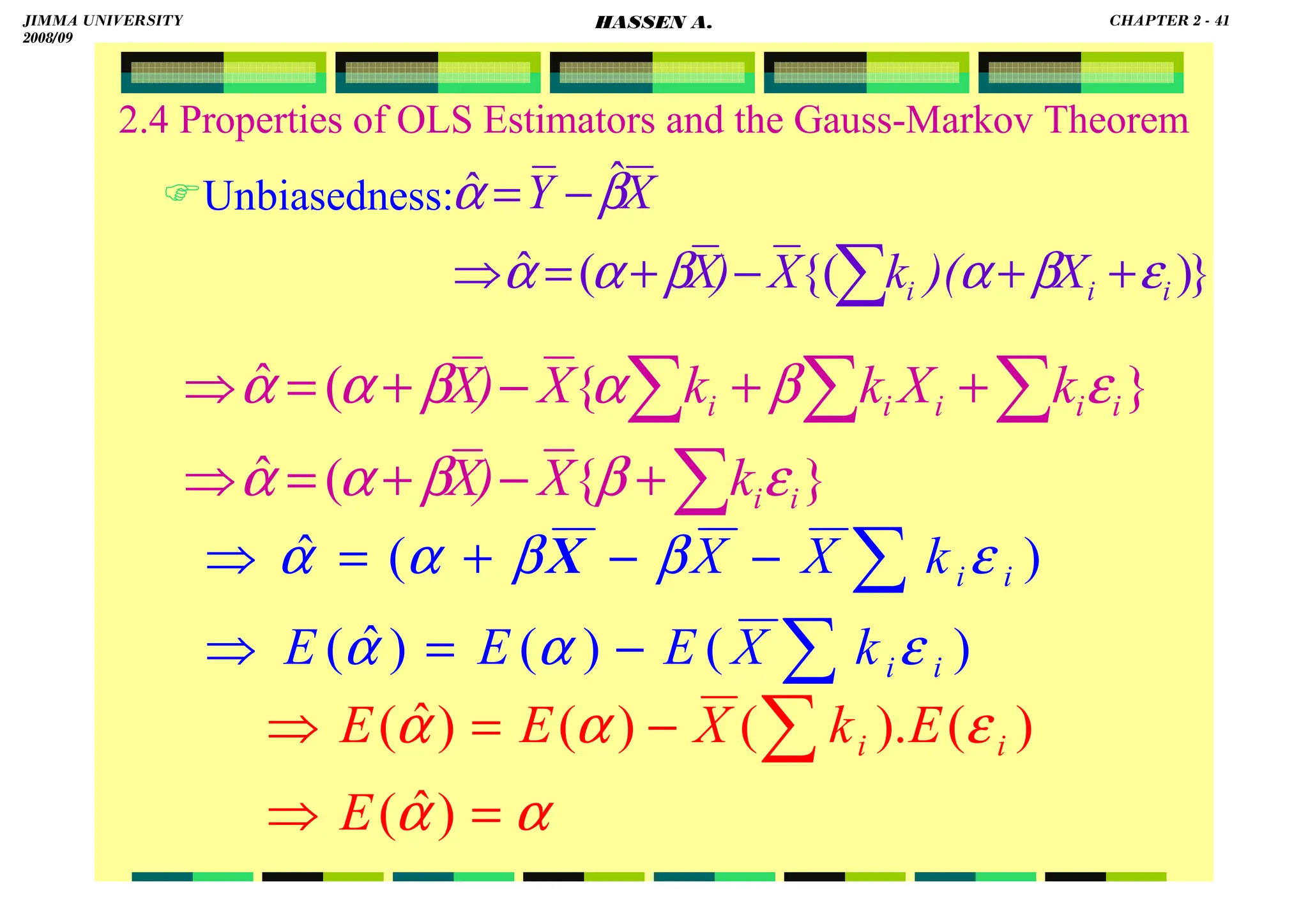
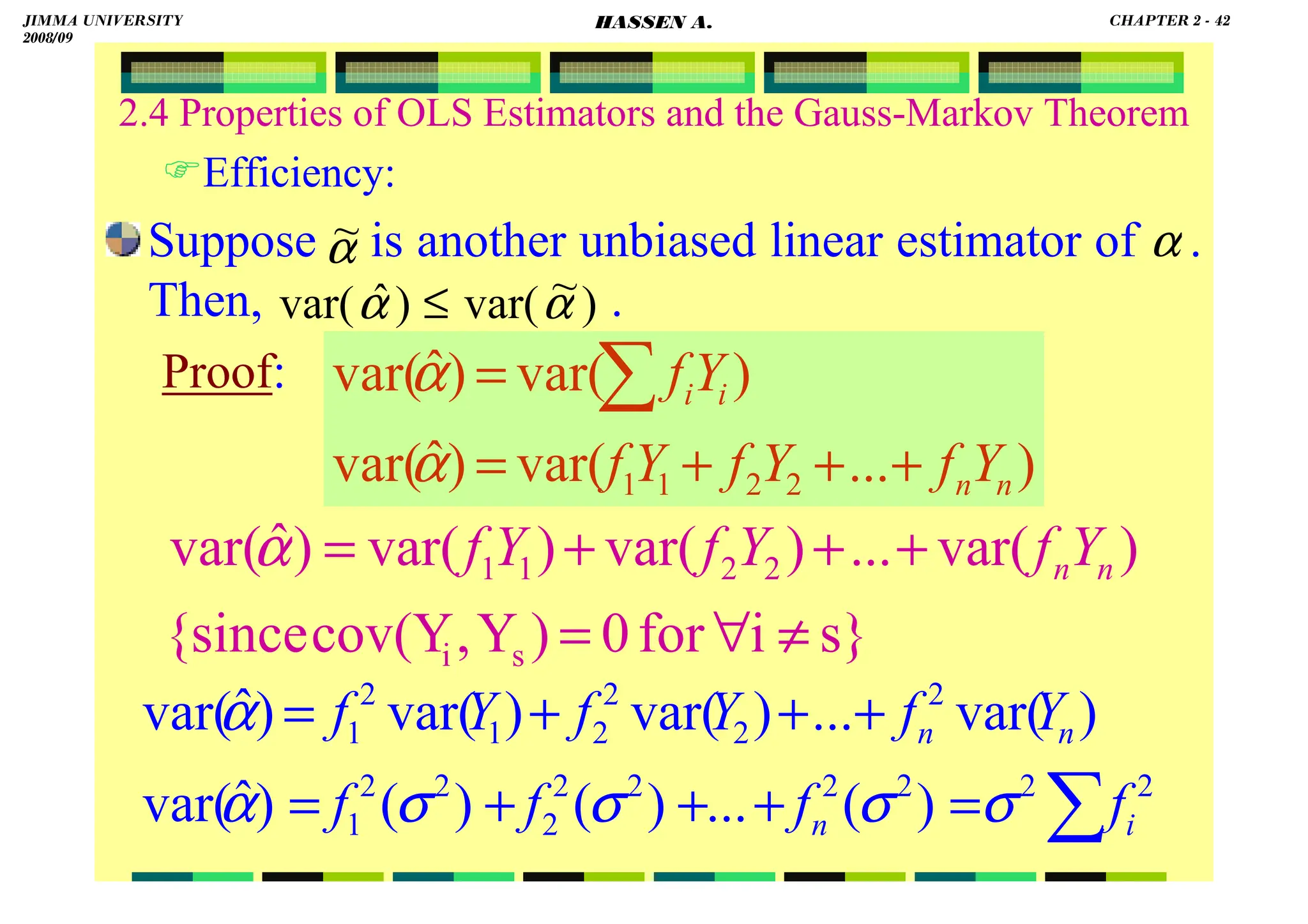
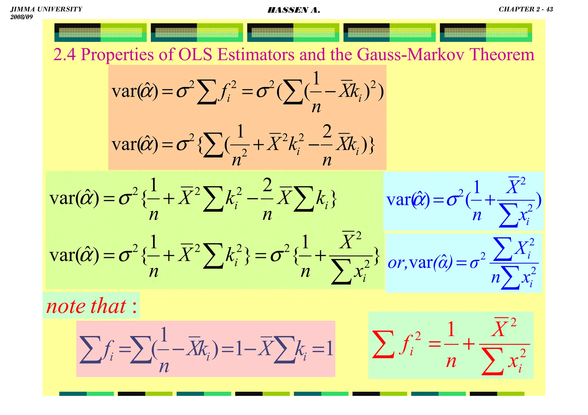
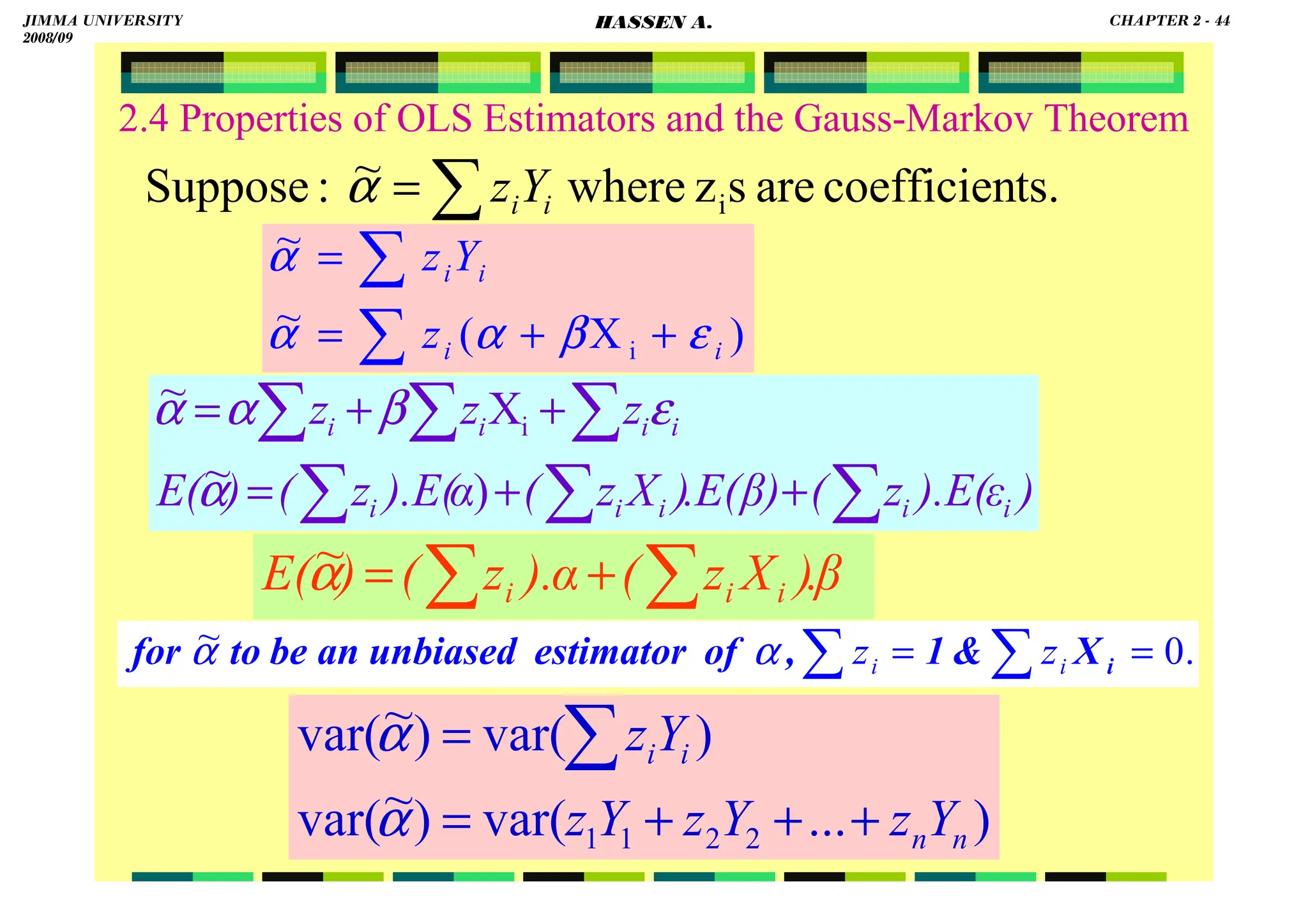
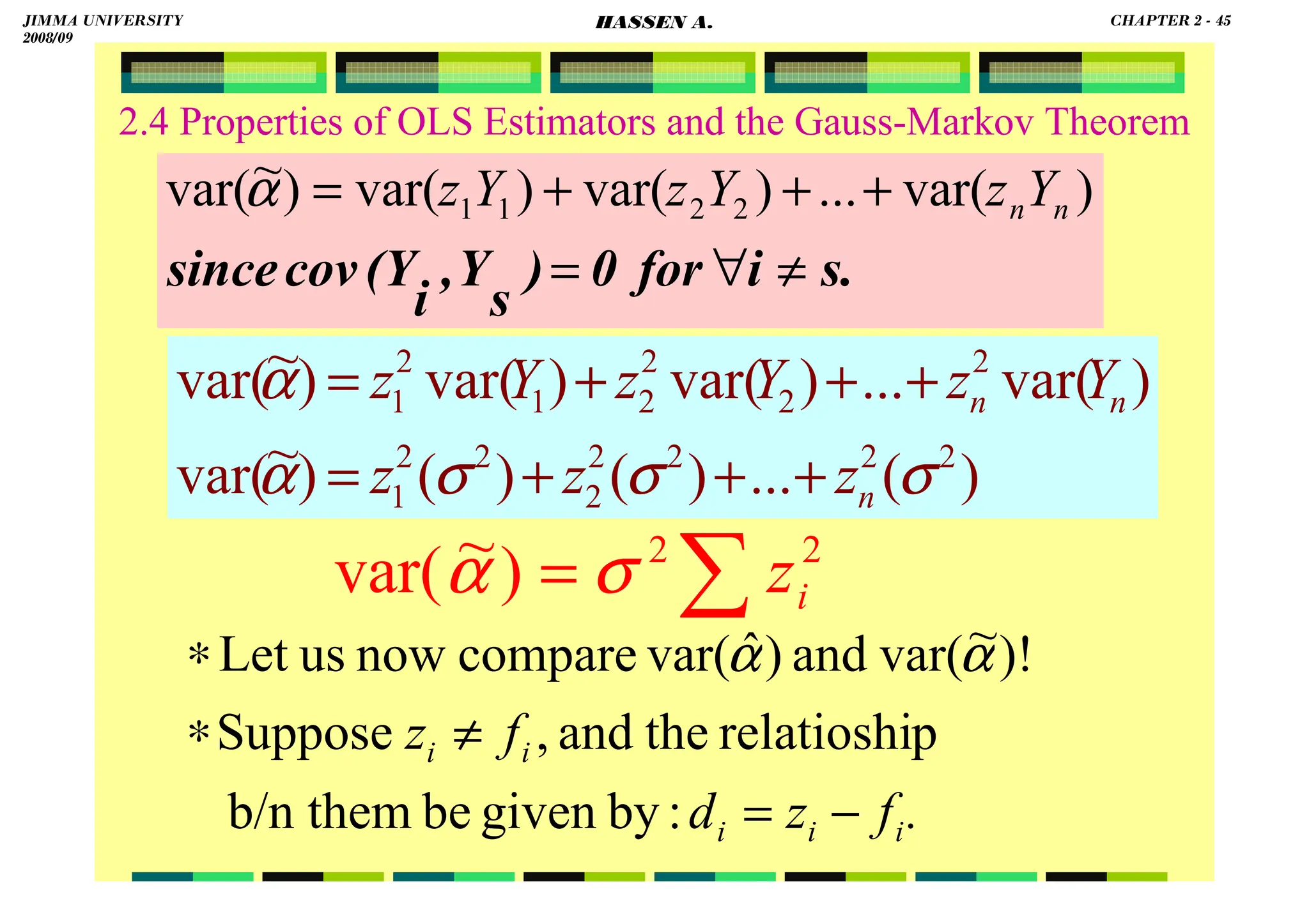
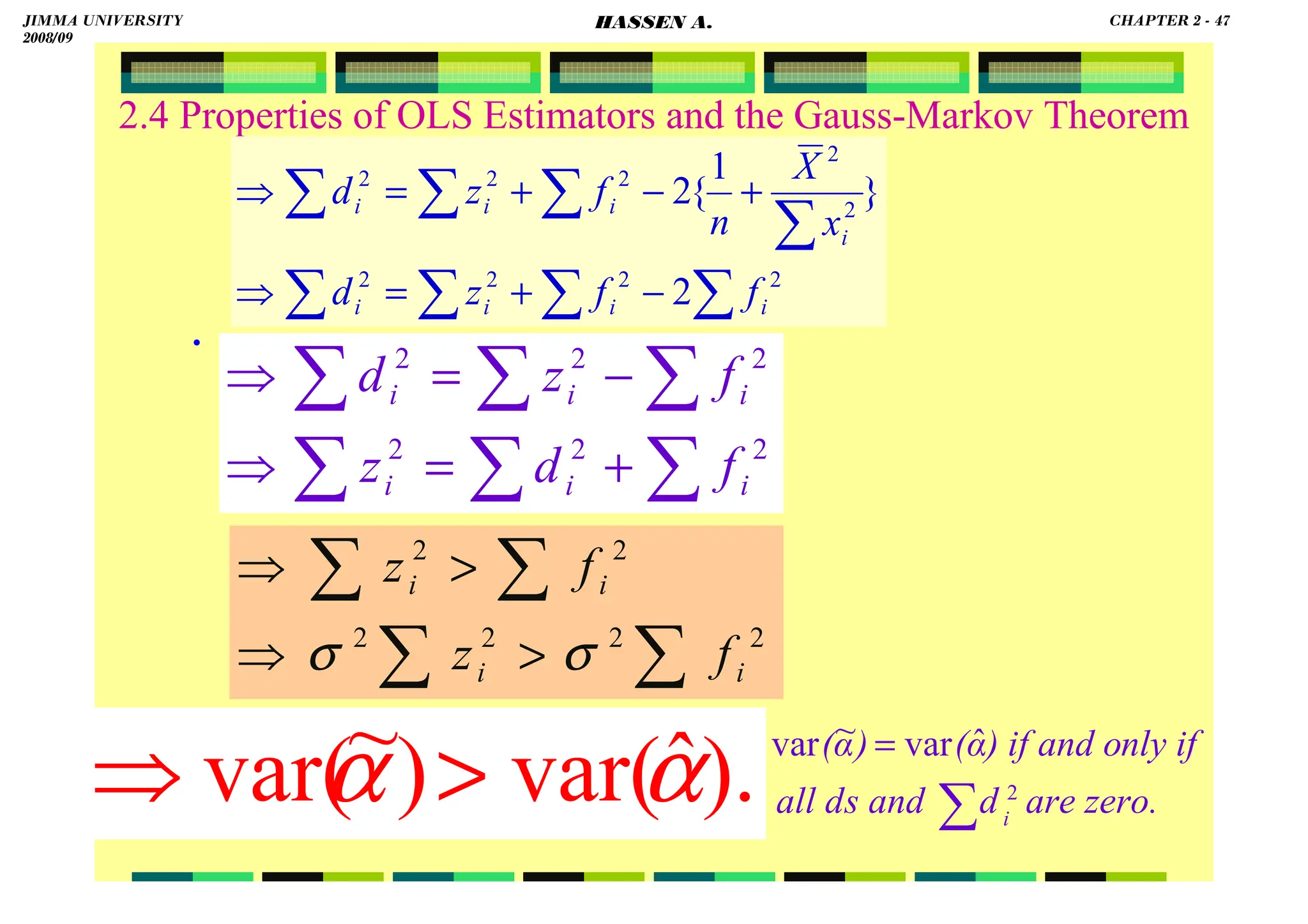
2.4 Properties of OLS Estimators and the Gauss-Markov Theorem
Note that:
(1) is a constant
(2)because xi is non-stochastic, ki is also nonstochastic
(3).
(4).
(5).
(6).
0
)
( 2
2
=
=
=
∑
∑
∑
∑
∑
i
i
i
i
i
x
x
x
x
k
1
)
(
)
( 2
2
2
=
=
=
∑
∑
∑
∑
∑
i
i
i
i
i
i
i
x
x
x
x
x
x
k
.
1
)
(
)]
[( 2
2
2
2
2
2
2
∑
∑
∑
∑
∑
∑ =
=
=
i
i
i
i
i
i
x
x
x
x
x
k
1
)
(
)
(
)
(
)
( 2
2
2
2
2
=
+
=
+
=
=
∑
∑
∑
∑
∑
∑
∑
∑
∑
i
i
i
i
i
i
i
i
i
i
i
i
x
x
X
x
x
X
x
x
x
X
x
x
X
k
∑ 2
i
x
JIMMA UNIVERSITY
2008/09
CHAPTER 2 - 33
HASSEN A.

47. HASSEN ABDA
2.4 Properties of OLS Estimators and the Gauss-Markov Theorem
Unbiasedness:
)
ˆ
ˆ
i
i
i
i
i
X
(
k
Y
k
ε
β
α
β
β
+
+
=
=
∑
∑
]
1
X
0
[
ˆ
X
ˆ
i
i
=
=
+
=
+
+
=
∑
∑
∑
∑
∑
∑
i
i
i
i
i
i
i
i
k
and
k
because
k
k
k
k
ε
β
β
ε
β
α
β
)
(
).
(
)
(
)
ˆ
(
)
...
(
)
(
)
ˆ
( 2
2
1
1
i
i
n
n
E
k
E
E
k
k
k
E
E
E
ε
β
β
ε
ε
ε
β
β
∑
+
=
+
+
+
+
=
β
β
β
β
=
+
= ∑
)
ˆ
(
)
0
).(
(
)
ˆ
(
E
k
E i
JIMMA UNIVERSITY
2008/09
CHAPTER 2 - 34
HASSEN A.

48. HASSEN ABDA
.
2.4 Properties of OLS Estimators and the Gauss-Markov Theorem
Efficiency:
Suppose is another unbiased linear estimator of .
Then, .
Proof:
)
...
var(
)
ˆ
var(
)
var(
)
ˆ
var(
2
2
1
1 n
n
i
i
Y
k
Y
k
Y
k
Y
k
+
+
+
=
= ∑
β
β
0}
s)
i
(for
Y
and
Y
between
covariance
the
{since
Y
k
Y
k
Y
k
s
i
n
n
=
≠
∀
+
+
+
= )
var(
...
)
var(
)
var(
)
ˆ
var( 2
2
1
1
β
)
(
...
)
(
)
(
)
ˆ
var(
)
var(
...
)
var(
)
var(
)
ˆ
var(
2
2
2
2
2
2
2
1
2
2
2
2
1
2
1
σ
σ
σ
β
β
n
n
n
k
k
k
Y
k
Y
k
Y
k
+
+
+
=
+
+
+
=
β
~
β
)
~
var(
)
ˆ
var( β
β ≤
JIMMA UNIVERSITY
2008/09
CHAPTER 2 - 35
HASSEN A.

49. HASSEN ABDA
2.4 Properties of OLS Estimators and the Gauss-Markov Theorem
∑
= 2
2
)
ˆ
var( i
k
σ
β
∑
= ts.
coefficien
are
s
w
where
Y
w
:
Suppose i
i
i
β
~
)
X
(
~
~
i i
i
i
i
w
Y
w
ε
β
α
β
β
+
+
=
=
∑
∑
β
.
)
X
w
(
).α
w
(
)
β
E( i
i
i
∑ ∑
+
=
~
)
ε
).E(
w
(
β)
.E(
)
X
w
(
).E(α
w
(
)
β
E(
w
w
w
i
i
i
i
i
i
i
i
i
∑
∑ ∑
∑
∑
∑
+
+
=
+
+
=
)
~
X
~
i ε
β
α
β
∑
= 2
2
)
ˆ
var(
i
x
or
σ
β
,
.
1
~
=
= ∑
∑ i
X
and
0
,
of
estimator
unbiased
an
be
to
for i
i w
w
β
β
JIMMA UNIVERSITY
2008/09
CHAPTER 2 - 36
HASSEN A.

50. HASSEN ABDA
2.4 Properties of OLS Estimators and the Gauss-Markov Theorem
.
)
...
var(
)
~
var(
)
var(
)
~
var(
2
2
1
1 n
n
i
i
Y
w
Y
w
Y
w
Y
w
+
+
+
=
= ∑
β
β
∑
= 2
2
)
~
var( i
w
σ
β
0
s)
i
(for
s
Y
and
i
Y
between
covariance
the
since =
≠
∀
+
+
+
= )
var(
...
)
var(
)
var(
)
~
var( 2
2
1
1 n
nY
w
Y
w
Y
w
β
)
(
...
)
(
)
(
)
~
var(
)
var(
...
)
var(
)
var(
)
~
var(
2
2
2
2
2
2
2
1
2
2
2
2
1
2
1
σ
σ
σ
β
β
n
n
n
w
w
w
Y
w
Y
w
Y
w
+
+
+
=
+
+
+
=
JIMMA UNIVERSITY
2008/09
CHAPTER 2 - 37
HASSEN A.

51. HASSEN ABDA
2.4 Properties of OLS Estimators and the Gauss-Markov Theorem
.
.
k
w
d
k
w
i
i
i
i
i
−
=
≠
∗
∗
:
by
given
be
them
b/n
r/p
the
and
,
Suppose
)!
β
var(
and
)
β
var(
compare
now
us
Let
~
ˆ
∑
∑
∑
∑
∑
=
−
=
⇒
∗
0
:
i
i
i
i
i
k
w
d
zero
equal
k
and
w
both
Because
∑
∑
∑
∑
∑ +
+
=
⇒
+
+
=
⇒
+
=
∗
)
)(
(
2
2
2
2
2
2
2
2
2
2
2
i
i
i
i
i
i
i
i
i
i
i
i
i
i
x
x
d
d
k
w
d
k
d
k
w
)
d
(k
)
(w
∑
∑
∑
∑
∑
=
−
=
−
=
⇒
∗
0
1
1
:
i
i
i
i
i
i
i
i
i
i
x
k
x
w
x
d
equal
x
k
and
x
w one
both
Because
JIMMA UNIVERSITY
2008/09
CHAPTER 2 - 38
HASSEN A.

52. HASSEN ABDA
39
2.4 Properties of OLS Estimators and the Gauss-Markov Theorem
.
).
β
(
)
β
( ˆ
var
~
var
⇒
∑
∑
∑
∑
∑
∑
∑
∑
∑
∑
∑
∑
+
=
⇒
+
+
=
⇒
+
+
=
⇒
2
2
2
2
2
2
2
2
2
2
2
)
0
)(
1
(
2
)
)(
1
(
2
i
i
i
i
i
i
i
i
i
i
i
i
i
d
k
w
x
d
k
w
x
d
x
d
k
w
∑
∑
⇒ 2
2
2
2
i
i k
w σ
σ
∑
∑
⇒ 2
2
i
i k
w ).
d
nd thus,
are zero a
s
d
, not all
k
(given w
i
i
i
i
0
2
≠
∑
.
d
and thus,
s are zero
d
nly if all
) if and o
β
(
)
β
i
i 0
ˆ
var
~
var(
2
=
=
∑
JIMMA UNIVERSITY
2008/09
CHAPTER 2 - 39
HASSEN A.

53. HASSEN ABDA
40
2.4 Properties of OLS Estimators and the Gauss-Markov Theorem
Linearity of : X
Y β
α ˆ
ˆ −
=
}
{
ˆ i
iY
k
X
Y ∑
−
=
⇒α
α
ˆ
}
...
{
ˆ 2
2
1
1 n
nY
k
Y
k
Y
k
X
Y +
+
+
−
=
⇒α
n
n Y
k
X
n
...
Y
k
X
n
Y
k
X
n
α )
1
(
)
1
(
)
1
(
ˆ 2
2
1
1 −
+
+
−
+
−
=
⇒
}
Y
k
X
...
Y
k
X
Y
k
X
{
Y
Y
Y
n
α n
n
n +
+
+
−
+
+
+
=
⇒ 2
2
1
1
2
1 )
...
(
1
ˆ
i
i
n
n k
X
n
f
where
Y
f
...
Y
f
Y
f
α −
=
+
+
+
=
⇒
1
ˆ 2
2
1
1
JIMMA UNIVERSITY
2008/09
CHAPTER 2 - 40
HASSEN A.

54. HASSEN ABDA
2.4 Properties of OLS Estimators and the Gauss-Markov Theorem
Unbiasedness:
}
)
{(
(
ˆ
ˆ
ˆ
∑ +
+
−
+
=
⇒
−
=
i
i
i X
)(
k
X
)
X
X
Y
ε
β
α
β
α
α
β
α
}
{
(
ˆ
}
{
(
ˆ
i
i
i
i
i
i
i
k
X
)
X
k
X
k
k
X
)
X
ε
β
β
α
α
ε
β
α
β
α
α
∑
∑
∑
∑
+
−
+
=
⇒
+
+
−
+
=
⇒
)
(
)
(
)
ˆ
(
)
(
ˆ
i
i
i
i
k
X
E
E
E
k
X
X
ε
α
α
ε
β
β
α
α
∑
∑
−
=
⇒
−
−
+
=
⇒ X
α
α
ε
α
α
=
⇒
−
=
⇒ ∑
)
ˆ
(
)
(
).
(
)
(
)
ˆ
(
E
E
k
X
E
E i
i
JIMMA UNIVERSITY
2008/09
CHAPTER 2 - 41
HASSEN A.

55. HASSEN ABDA
2.4 Properties of OLS Estimators and the Gauss-Markov Theorem
Efficiency:
Suppose is another unbiased linear estimator of .
Then, .
Proof:
)
...
var(
)
ˆ
var(
)
var(
)
ˆ
var(
2
2
1
1 n
n
i
i
Y
f
Y
f
Y
f
Y
f
+
+
+
=
= ∑
α
α
s}
i
for
0
)
Y
,
cov(Y
{since
)
var(
...
)
var(
)
var(
)
ˆ
var(
s
i
2
2
1
1
≠
∀
=
+
+
+
= n
nY
f
Y
f
Y
f
α
∑
=
+
+
+
=
+
+
+
=
2
2
2
2
2
2
2
2
2
1
2
2
2
2
1
2
1
)
(
...
)
(
)
(
)
ˆ
var(
)
var(
...
)
var(
)
var(
)
ˆ
var(
i
n
n
n
f
f
f
f
Y
f
Y
f
Y
f
σ
σ
σ
σ
α
α
α
~ α
)
~
var(
)
ˆ
var( α
α ≤
JIMMA UNIVERSITY
2008/09
CHAPTER 2 - 42
HASSEN A.

56. HASSEN ABDA
43
2.4 Properties of OLS Estimators and the Gauss-Markov Theorem
)}
2
1
(
{
)
ˆ
var(
)
)
1
(
(
)
ˆ
var(
2
2
2
2
2
2
2
2
i
i
i
i
k
X
n
k
X
n
k
X
n
f
∑
∑
∑
−
+
=
−
=
=
σ
α
σ
σ
α
∑
∑
= 2
2
2
ˆ
var
i
i
x
n
X
σ
)
α
(
or,
}
1
{
}
1
{
)
ˆ
var(
}
2
1
{
)
ˆ
var(
2
2
2
2
2
2
2
2
2
∑
∑
∑
∑
+
=
+
=
−
+
=
i
i
i
i
x
X
n
k
X
n
k
X
n
k
X
n
σ
σ
α
σ
α
1
1
)
1
( =
−
=
−
= ∑
∑
∑ i
i
i k
X
k
X
n
f
∑
∑ +
= 2
2
2 1
i
i
x
X
n
f
:
that
note
)
1
(
)
ˆ
var( 2
2
2
∑
+
=
i
x
X
n
σ
α
JIMMA UNIVERSITY
2008/09
CHAPTER 2 - 43
HASSEN A.

57. HASSEN ABDA
2.4 Properties of OLS Estimators and the Gauss-Markov Theorem
)
ε
).E(
z
(
β)
.E(
)
X
z
(
).E(α
z
(
)
E(
z
z
z
i
i
i
i
i
i
i
i
i
∑
∑ ∑
∑
∑
∑
+
+
=
+
+
=
)
~
X
~
i
α
ε
β
α
α
)
...
var(
)
~
var(
)
var(
)
~
var(
2
2
1
1 n
n
i
i
Y
z
Y
z
Y
z
Y
z
+
+
+
=
= ∑
α
α
β
.
)
X
z
(
).α
z
(
)
E( i
i
i
∑ ∑
+
=
α
~
)
X
(
~
~
i i
i
i
i
z
Y
z
ε
β
α
α
α
+
+
=
=
∑
∑
∑
= ts.
coefficien
are
s
z
where
~
:
Suppose i
i
iY
z
α
.
0
~ =
= ∑
∑ i
X
1
,
of
estimator
unbiased
an
be
to
for i
i z
z
α
α
JIMMA UNIVERSITY
2008/09
CHAPTER 2 - 44
HASSEN A.

58. HASSEN ABDA
2.4 Properties of OLS Estimators and the Gauss-Markov Theorem
.
∑
= 2
2
)
~
var( i
z
σ
α
s.
i
for
0
)
s
Y
,
i
(Y
cov
since ≠
∀
=
+
+
+
= )
var(
...
)
var(
)
var(
)
~
var( 2
2
1
1 n
nY
z
Y
z
Y
z
α
)
(
...
)
(
)
(
)
~
var(
)
var(
...
)
var(
)
var(
)
~
var(
2
2
2
2
2
2
2
1
2
2
2
2
1
2
1
σ
σ
σ
α
α
n
n
n
z
z
z
Y
z
Y
z
Y
z
+
+
+
=
+
+
+
=
.
f
z
d
f
z
i
i
i
i
i
−
=
≠
∗
∗
:
by
given
be
b/n them
p
relatioshi
the
and
,
Suppose
)!
~
var(
and
)
ˆ
var(
compare
now
us
Let α
α
JIMMA UNIVERSITY
2008/09
CHAPTER 2 - 45
HASSEN A.

59. HASSEN ABDA
2.4 Properties of OLS Estimators and the Gauss-Markov Theorem
.
X
X
z
X
X
z
X
z
X
z
X
X
z
x
z
z
X
z
i
i
i
i
i
i
i
i
i
i
i
i
i
−
=
−
=
−
=
−
=
−
=
⇒
=
=
∗
∑
∑
∑
∑
∑
∑
∑
∑
)
1
(
0
)
(
,
1
and
0,
Because
)}
)(
(
1
{
2
)}
)(
(
1
{
2
2
2
2
2
2
2
2
2
X
x
X
n
f
z
d
x
z
x
X
z
n
f
z
d
i
i
i
i
i
i
i
i
i
i
i
−
−
−
+
=
⇒
−
−
+
=
⇒
∑
∑
∑
∑
∑
∑
∑
∑
∑
∑
}
{
2
2
2
2
∑
∑
∑
∑ −
+
= i
i
i
i
i f
z
f
z
d )
(
1
2
∑
−
=
i
i
i
x
x
X
n
f
where
]}
)
1
(
[
{
2 2
2
2
2
∑
∑
∑
∑
∑ −
−
+
=
i
i
i
i
i
i
x
x
X
n
z
f
z
d
JIMMA UNIVERSITY
2008/09
CHAPTER 2 - 46
HASSEN A.

60. HASSEN ABDA
2.4 Properties of OLS Estimators and the Gauss-Markov Theorem
.
).
ˆ
var(
)
~
var( α
α
⇒
∑
∑
∑
∑
∑
∑
+
=
⇒
−
=
⇒
2
2
2
2
2
2
i
i
i
i
i
i
f
d
z
f
z
d
∑
∑
∑
∑
⇒
⇒
2
2
2
2
2
2
i
i
i
i
f
z
f
z
σ
σ
∑
∑
∑
∑
∑
∑
∑
∑
−
+
=
⇒
+
−
+
=
⇒
2
2
2
2
2
2
2
2
2
2
}
1
{
2
i
i
i
i
i
i
i
i
f
f
z
d
x
X
n
f
z
d
are zero.
d
s and
all d
nly if
) if and o
α
(
)
α
(
i
∑
=
2
ˆ
var
~
var
JIMMA UNIVERSITY
2008/09
CHAPTER 2 - 47
HASSEN A.

61. HASSEN ABDA
2.5 Residuals and Goodness of Fit
Decomposing the variation in Y:
JIMMA UNIVERSITY
2008/09
CHAPTER 2 - 48
HASSEN A.

62. HASSEN ABDA
2.5 Residuals and Goodness of Fit
Decomposing the variation in Y:
One measure of the variation in Y is the sum of its
squared deviations around its sample mean, often
described as the Total Sum of Squares, TSS.
TSS, the total sum of squares of Y can be
decomposed into ESS, the ‘explained’ sum of
squares, and RSS, the residual (‘unexplained’) sum
of squares.
TSS = ESS + RSS
∑
∑
∑ +
−
=
− 2
2
2 ˆ
i
i
i e
)
Y
Y
(
)
Y
(Y
JIMMA UNIVERSITY
2008/09
CHAPTER 2 - 49
HASSEN A.

63. HASSEN ABDA
2.5 Residuals and Goodness of Fit
The last term equals zero:
i
i
i e
Y
Y
Y
Y +
−
=
−
⇒ ˆ
i
i
i e
Y
Y +
= ˆ
2
2
)
ˆ
(
)
( i
i
i e
Y
Y
Y
Y +
−
=
−
∑
∑ +
−
=
− 2
2
)
ˆ
(
)
( i
i
i e
Y
Y
Y
Y
∑
∑ +
= 2
2
)
ˆ
( i
i
i e
y
y
∑
∑
∑
∑ +
+
= i
i
i
i
i e
y
e
y
y ˆ
2
ˆ 2
2
2
∑
∑
∑
∑ −
=
−
= i
i
i
i
i
i
i e
Y
e
Y
e
Y
Y
e
y ˆ
)
ˆ
(
ˆ
∑
∑
∑ −
+
=
⇒ i
i
i
i
i e
Y
e
X
e
y )
ˆ
ˆ
(
ˆ β
α
JIMMA UNIVERSITY
2008/09
CHAPTER 2 - 50
HASSEN A.

64. HASSEN ABDA
2.5 Residuals and Goodness of Fit
.
Hence:
Coefficient of Determination (R2):
the proportion of the variation in the dependent
variable that is explained by the model.
∑
∑
∑ +
=
⇒ 2
2
2
ˆ i
i
i
e
y
y
RSS
ESS
TSS +
=
∑
∑
∑ +
=
⇒ i
i
i
i
i e
X
e
e
y β
α ˆ
ˆ
ˆ
0
ˆ =
⇒∑ i
ie
y
65
.
14
75
.
15
4
.
30 +
=
JIMMA UNIVERSITY
2008/09
CHAPTER 2 - 51
HASSEN A.

65. HASSEN ABDA
52
2.5 Residuals and Goodness of Fit
The OLS regression coefficients are chosen in such
a way as to minimize the sum of the squares of the
residuals. Thus it automatically follows that they
maximize R2.
∑
∑
=
= 2
2
2
ˆ
.
1
y
y
TSS
ESS
R
TSS
RSS
TSS
ESS
TSS
TSS
RSS
ESS
TSS
+
=
⇒
+
=
∑
∑
−
=
⇒ 2
2
2
1
.
3
y
e
R
i
∑
∑
=
= 2
2
2
)
ˆ
(
y
x
TSS
ESS
R
β
∑
∑
=
= 2
2
2
2 ˆ
.
2
y
x
TSS
ESS
R β
TSS
RSS
TSS
ESS
TSS
RSS
TSS
ESS
−
=
⇒
+
=
⇒
1
1
JIMMA UNIVERSITY
2008/09
CHAPTER 2 - 52
HASSEN A.

66. HASSEN ABDA
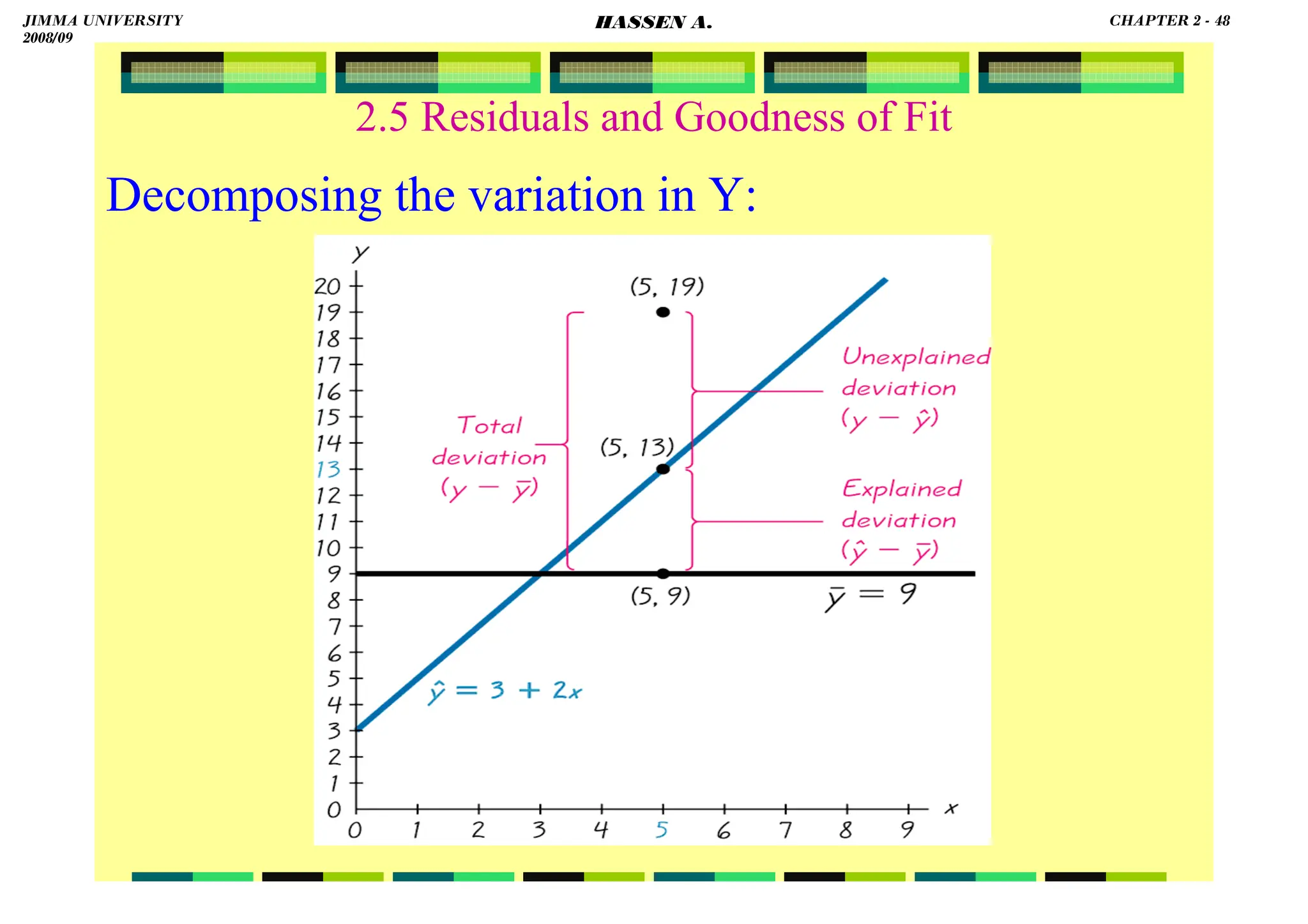
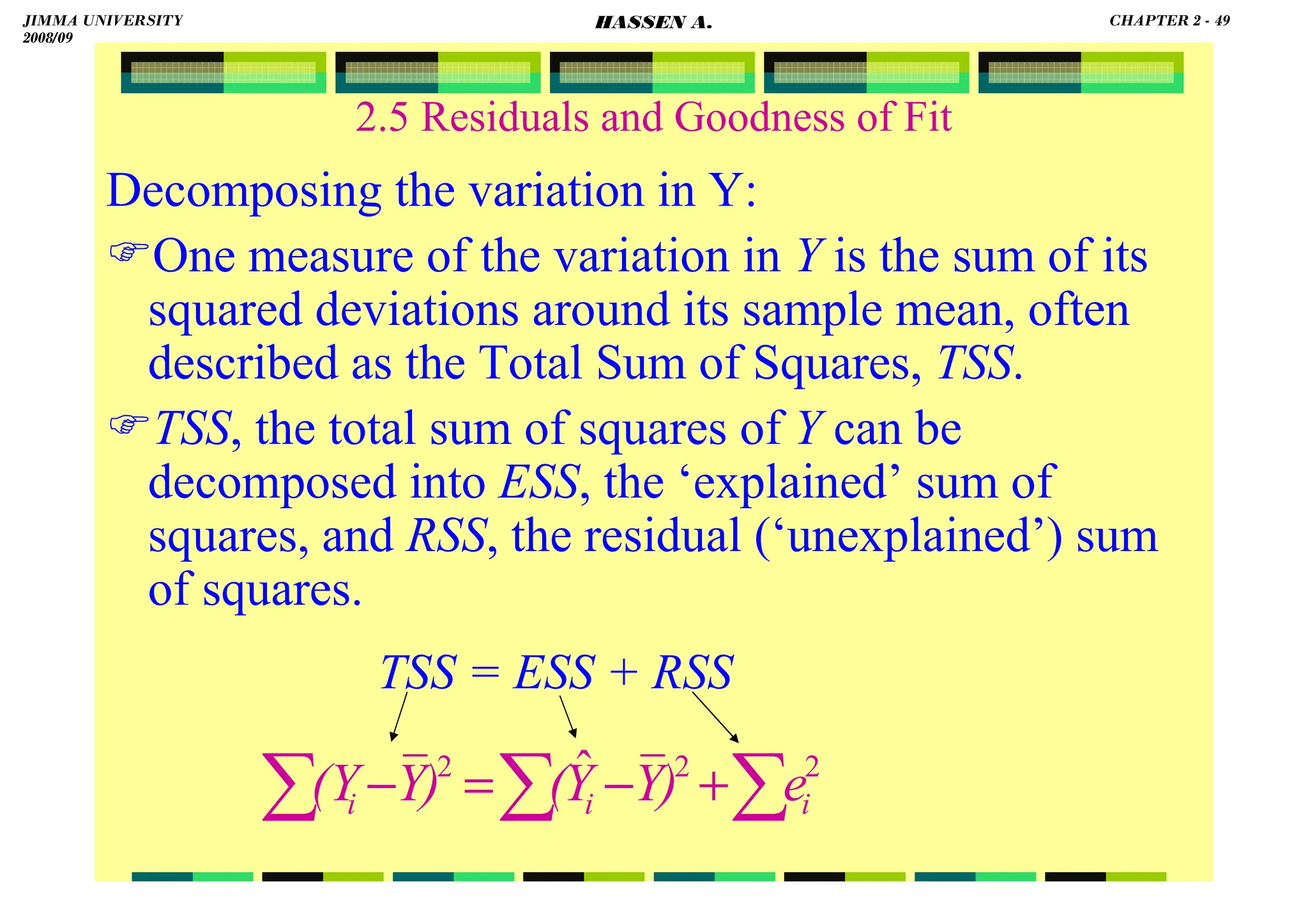
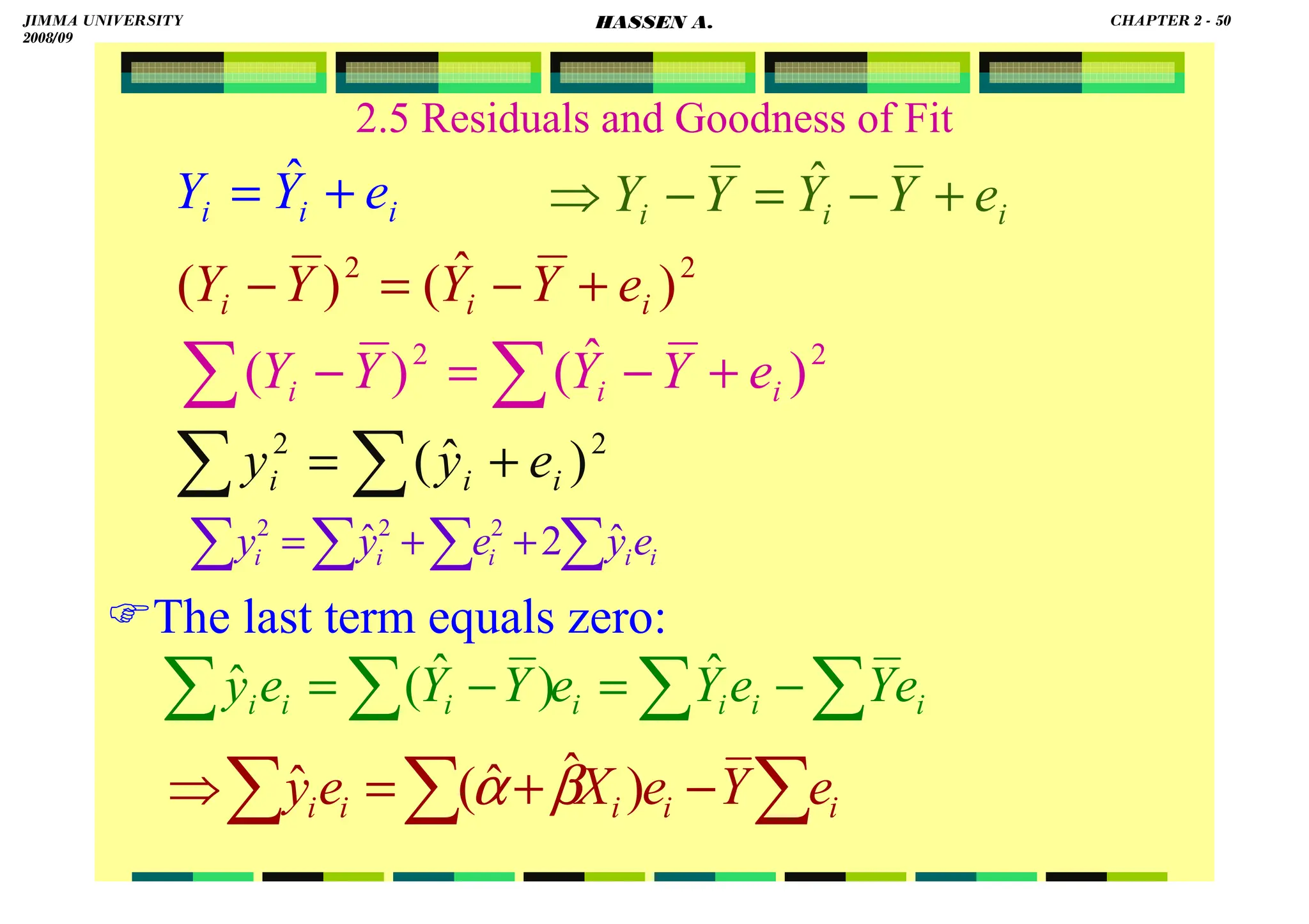
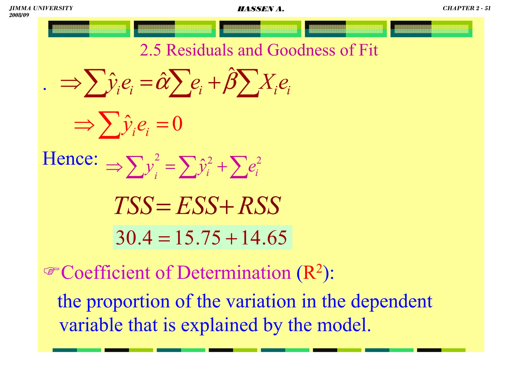
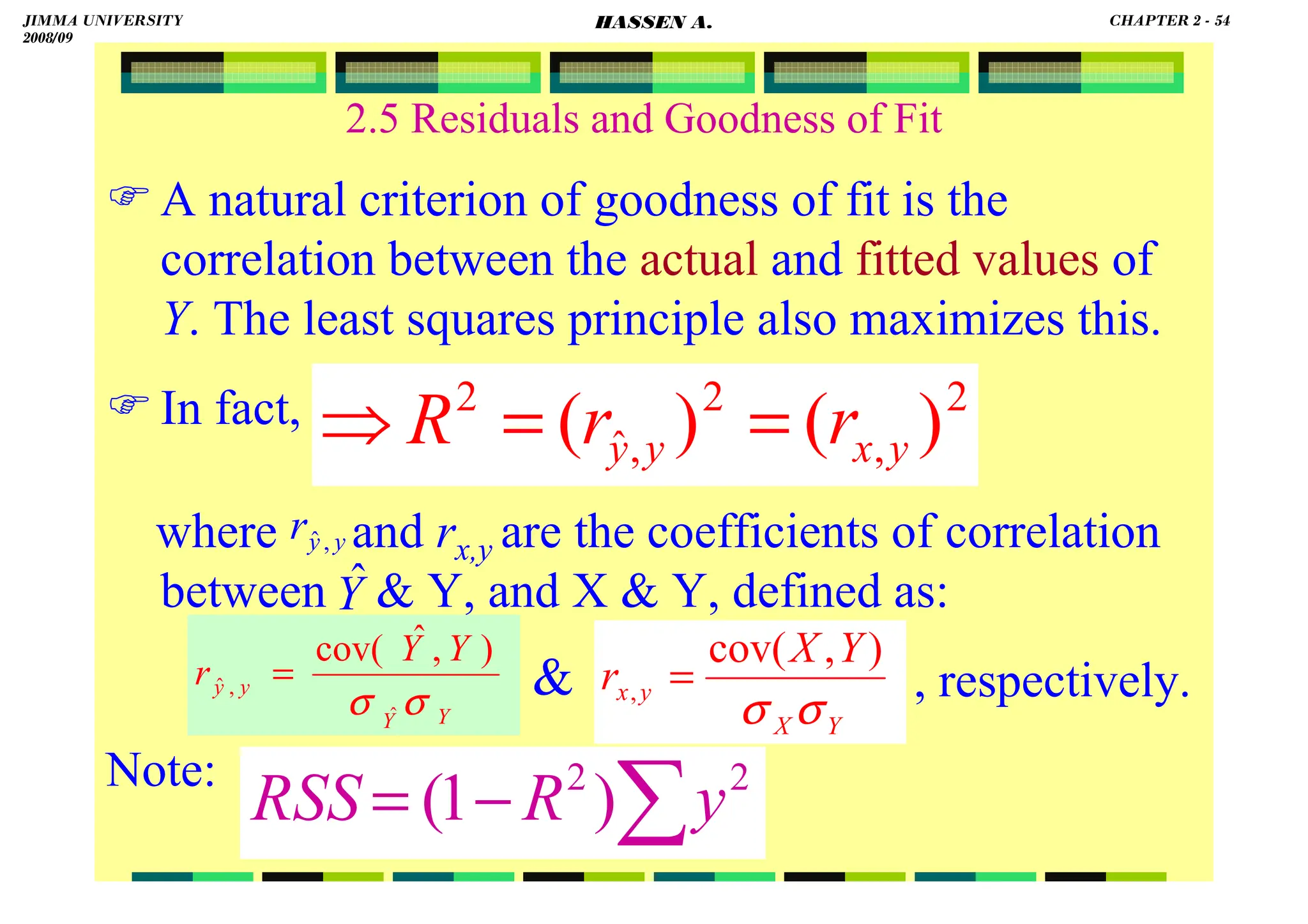
2.5 Residuals and Goodness of Fit
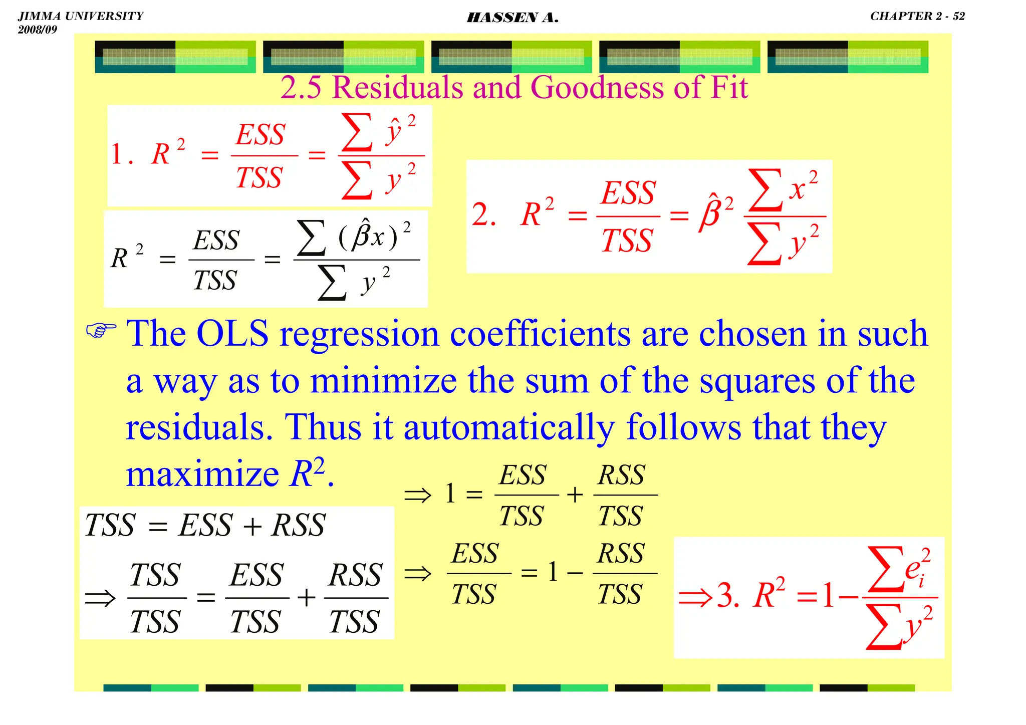
Coefficient of Determination (R2):
∑
∑
∑
∑
= 2
2
2
y
xy
x
xy
R
∑ ∑
∑
=
⇒ 2
2
2
2
)
(
.
5
y
x
xy
R
)
)(
(
ˆ
2
2
2
2
∑
∑
∑
∑
=
=
y
x
x
xy
TSS
ESS
R β
∑
∑
=
= 2
2 ˆ
.
4
y
xy
TSS
ESS
R β
)
var(
)
var(
)]
,
[cov(
.
6
2
2
Y
X
Y
X
R
×
=
⇒
5181
.
0
4
.
30
75
.
15
ˆ
2
2
2
=
=
=
=
∑
∑
y
y
TSS
ESS
R
i
JIMMA UNIVERSITY
2008/09
CHAPTER 2 - 53
HASSEN A.

67. HASSEN ABDA
2.5 Residuals and Goodness of Fit
A natural criterion of goodness of fit is the
correlation between the actual and fitted values of
Y. The least squares principle also maximizes this.
In fact,
where and rx,y are the coefficients of correlation
between Y, and X Y, defined as:
, respectively.
Note:
∑
−
= 2
2
)
1
( y
R
RSS
2
,
2
,
ˆ
2
)
(
)
( y
x
y
y r
r
R =
=
⇒
Y
X
r
Y
X
y
x
σ
σ
)
,
cov(
, =
Y
Y
y
y
Y
Y
r
σ
σ ˆ
,
ˆ
)
,
ˆ
cov(
=
y
y
r ,
ˆ
Y
ˆ
JIMMA UNIVERSITY
2008/09
CHAPTER 2 - 54
HASSEN A.

68. HASSEN ABDA
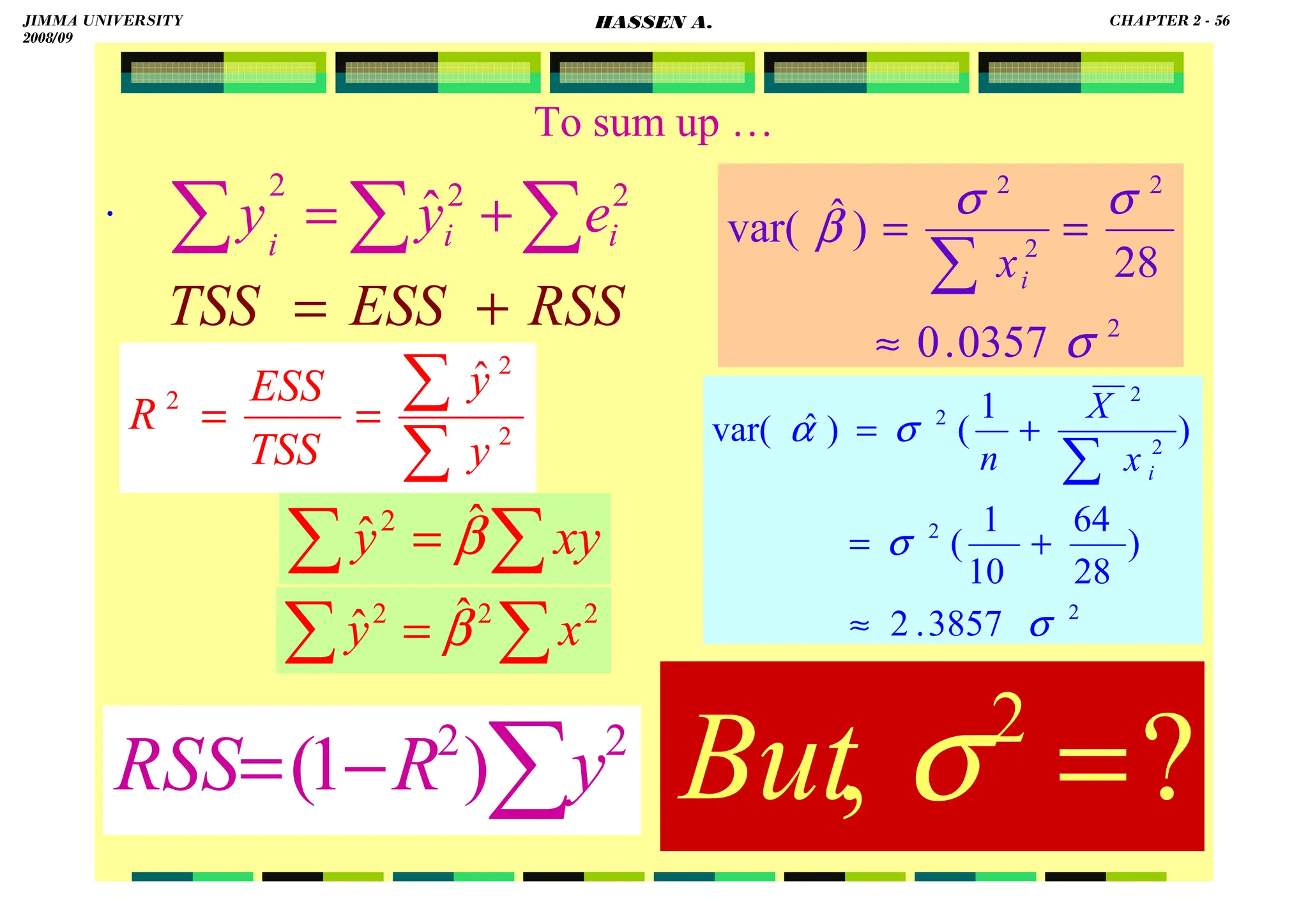
55
To sum up:
Use
OLS:
Given the assumptions of the linear regression
model, the estimators have the smallest
variance of all linear and unbiased estimators of
.
i
i X
X
Y
E
estimate
to
i
X
i
Y β
α
β
α +
=
+
= ]
|
[
ˆ
ˆ
ˆ
∑ ∑ −
−
=
−
=
= =
=
∑
n
i
n
i
i
i
i
i
n
i
i )
X
β
α
(Y
)
Y
(Y
e
1 1
2
2
1
2 ˆ
ˆ
ˆ
β̂
,
α̂
min
∑
∑
= 2
ˆ
x
xy
β X
β
Y
α ˆ
ˆ −
=
β
α ˆ
ˆ and
β
α and
∑
= 2
2
)
ˆ
var(
i
x
σ
β )
1
(
)
ˆ
var( 2
2
2
∑
+
=
i
x
X
n
σ
α
∑
∑
= 2
2
2
i
i
x
n
X
σ
JIMMA UNIVERSITY
2008/09
CHAPTER 2 - 55
HASSEN A.

69. HASSEN ABDA
56
To sum up …
.
2
2
2
2
0357
.
0
28
)
ˆ
var(
σ
σ
σ
β
≈
=
=
∑ i
x
∑
∑
∑ +
= 2
2
2
ˆ i
i
i
e
y
y
RSS
ESS
TSS +
=
∑
∑
=
= 2
2
2
ˆ
y
y
TSS
ESS
R
∑
−
= 2
2
)
1
( y
R
RSS
2
2
2
2
2
3857
.
2
)
28
64
10
1
(
)
1
(
)
ˆ
var(
σ
σ
σ
α
≈
+
=
+
=
∑ i
x
X
n
?
, 2
=
σ
But
∑
∑ = xy
y β̂
ˆ2
∑
∑ = 2
2
2 ˆ
ˆ x
y β
JIMMA UNIVERSITY
2008/09
CHAPTER 2 - 56
HASSEN A.

70. HASSEN ABDA
2
2
)
2
(
)
(
)
( σ
−
=
= ∑ n
e
E
RSS
E i
.
2
ˆ 2
2
2
σ
σ of
estimator
unbiased
an
is
−
=
⇒
∑
n
ei
:
then
,
2
ˆ
define
we
if
Thus,
2
2
−
=
∑
n
ei
σ
An unbiased estimator for σ2
2
2
2
2
)
2
)(
2
1
(
)
(
)
2
1
(
)
ˆ
( σ
σ
σ =
−
−
=
−
= ∑ n
n
e
E
n
E i
JIMMA UNIVERSITY
2008/09
CHAPTER 2 - 57
HASSEN A.

71. HASSEN ABDA
2.6 Confidence Intervals and Hypothesis Testing in Regression Analysis
Why is the Error Normality Assumption Important?
The normality assumption permits us to derive the
functional form of the sampling distributions of
.
Knowing the form of the sampling distributions
enables us to derive feasible test statistics for the
OLS coefficient estimators.
These feasible test statistics enable us to conduct
statistical inference, i.e.,
1)to construct confidence intervals for .
2)to test hypothesis about the values of .
2
ˆ
ˆ
,
ˆ σ
β
α
2
, σ
β
α
2
, σ
β
α
JIMMA UNIVERSITY
2008/09
CHAPTER 2 - 58
HASSEN A.

72. HASSEN ABDA
59
2.6 Confidence Intervals and Hypothesis Testing in Regression Analysis
. )
,
0
(
~ 2
σ
ε N
i
)
,
(
~ 2
σ
β
α i
i X
N
Y +
⇒
)
,
(
~
ˆ
2
2
∑ i
x
N
σ
β
β )
,
(
~
ˆ 2
2
2
∑
∑
i
i
x
X
N σ
α
α
2
ˆ
ˆ
ˆ
−
−
n
~t
)
β
(
e
s
β
β
∑
=
2
ˆ
)
ˆ
(
ˆ
i
x
e
s
σ
β
2
~
)
ˆ
(
ˆ
ˆ
−
−
n
t
e
s α
α
α
∑
∑
= 2
2
.
ˆ
ˆ
ˆ
i
i
x
n
X
σ
)
α
(
e
s
2
ˆ
2
−
∑
=
n
e
σ i
)
1
,
0
(
~
)
ˆ
( 2
N
xi
∑
−
σ
β
β
JIMMA UNIVERSITY
2008/09
CHAPTER 2 - 59
HASSEN A.

73. HASSEN ABDA
2.6 Confidence Intervals and Hypothesis Testing in Regression Analysis
Confidence Interval for :
Similarly,
α
α
α −
=
≤
≤
− −
− −
1
}
)
(
ˆ
{ 2
2
/
2
2
/
ˆ
ˆ n
n
t
e
s
t
P
αααα
αααα
αααα
)
(
e
)s
(tn
α/
αααα
αααα
ˆ
ˆ ˆ
2
2
−
±
::::
αααα
CI for
ided
α)% Two-S
( −
1
100
:
CI for
ided
α)% Two-S
(
β
−
1
100
)
(
ˆ
)
( ˆ
ˆ 2
2
/ β
β α e
s
tn−
±
α and β
JIMMA UNIVERSITY
2008/09
CHAPTER 2 - 60
HASSEN A.

74. HASSEN ABDA
2.6 Confidence Intervals and Hypothesis Testing in Regression Analysis
CI for :
2
2
2
2
~
ˆ
)
2
( −
− n
n χ
σ
σ
α
χ
χ
χ α
α −
=
≤
≤
− 1
}
{ 2
);
2
/
(
2
2
);
2
/
(
1 df
df
df
P
2
σ
α
χ
σ
σ
χ α
α −
=
≤
−
≤
⇒ −
−
− 1
}
ˆ
)
2
(
{ 2
)
2
(
);
2
/
(
2
2
2
)
2
(
);
2
/
(
1 n
n
n
P
α
χ
σ
σ
χ α
α
−
=
≥
−
≥
⇒
−
−
−
1
}
1
ˆ
)
2
(
1
{ 2
)
2
(
);
2
/
(
2
2
2
)
2
(
);
2
/
(
1 n
n n
P
α
}
χ
σ
)
(n
σ
χ
P{
)
);(n
(α
)
);(n
(α
−
=
≤
−
≤
⇒
−
−
−
1
1
ˆ
2
1
2
2
2
/
1
2
2
2
2
2
/
JIMMA UNIVERSITY
2008/09
CHAPTER 2 - 61
HASSEN A.

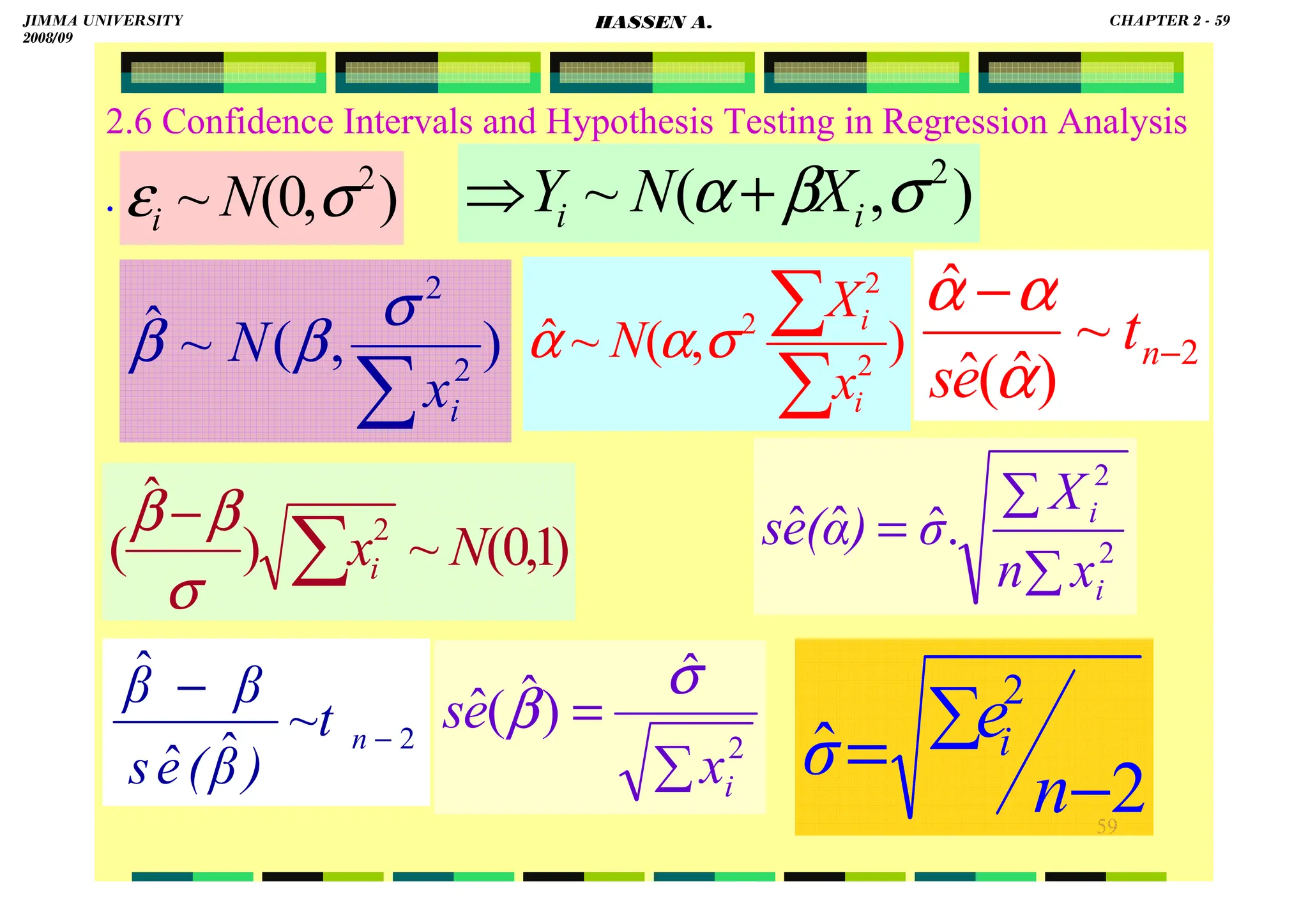
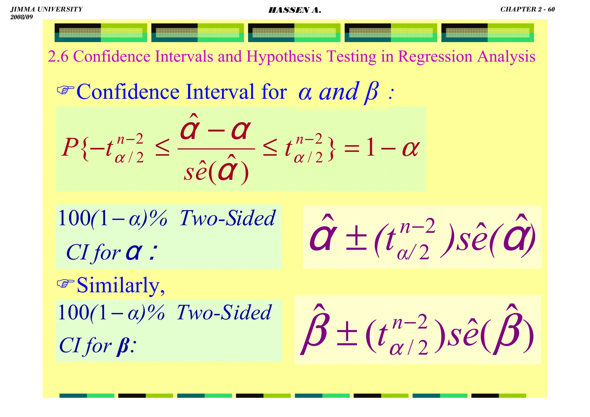
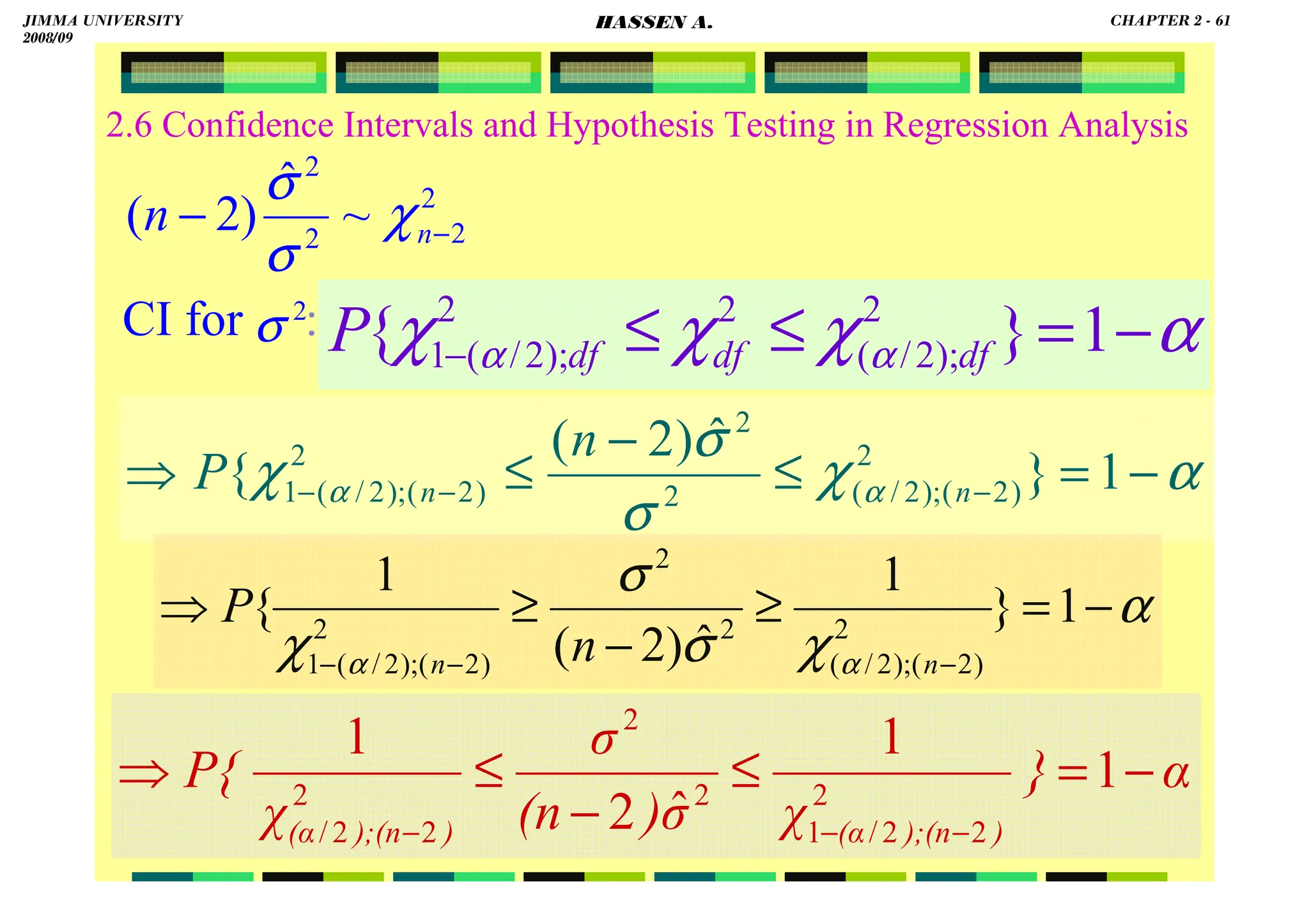
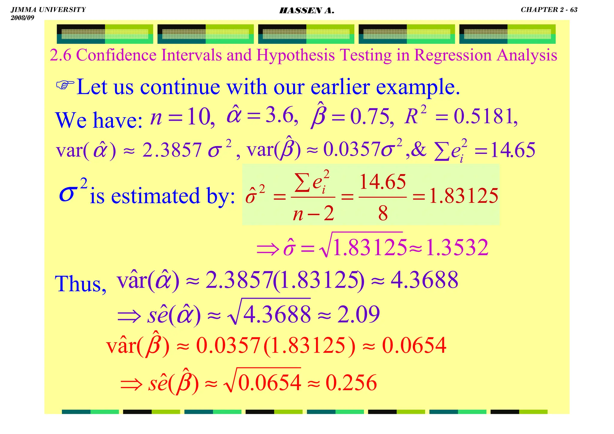
75. HASSEN ABDA
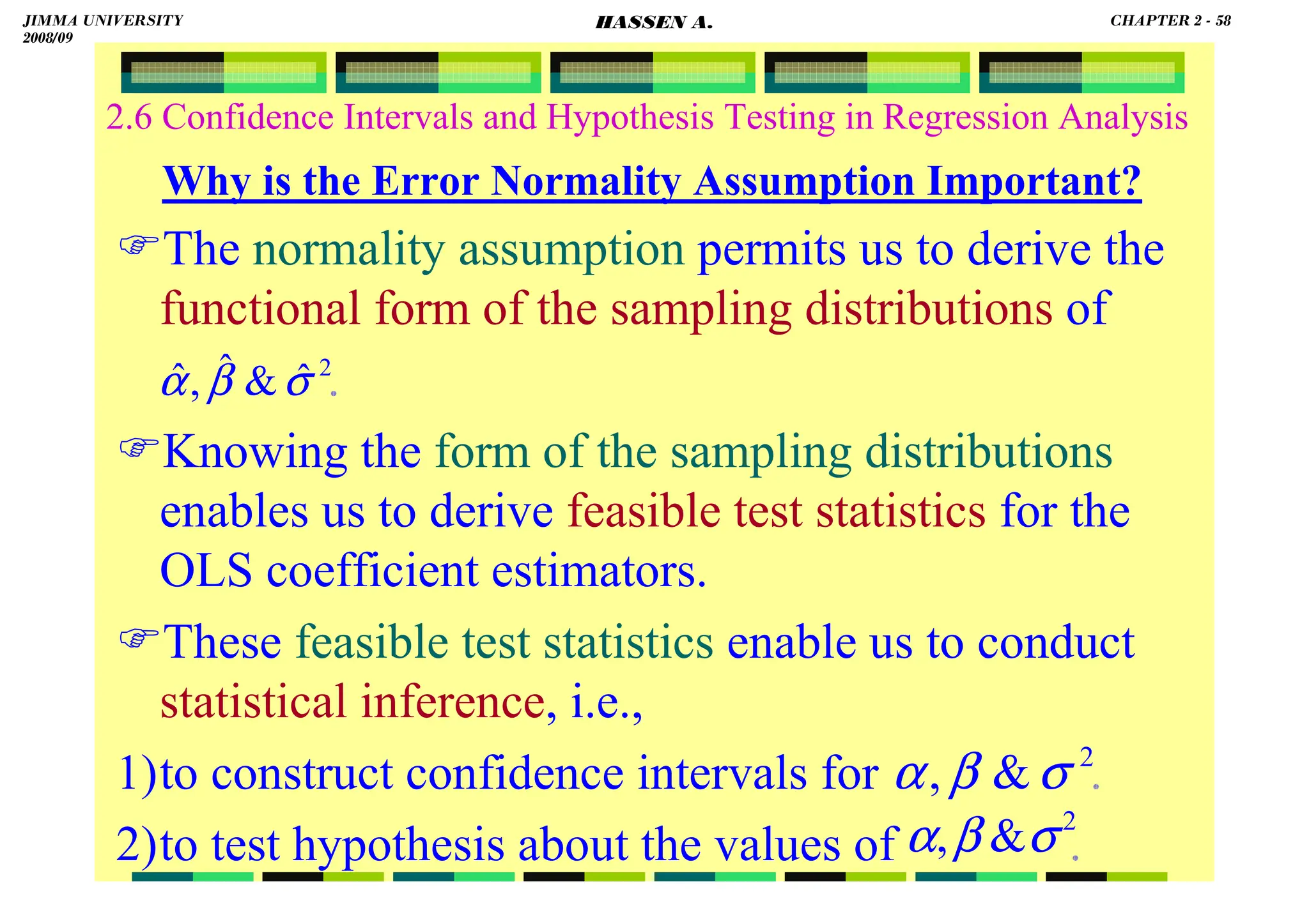
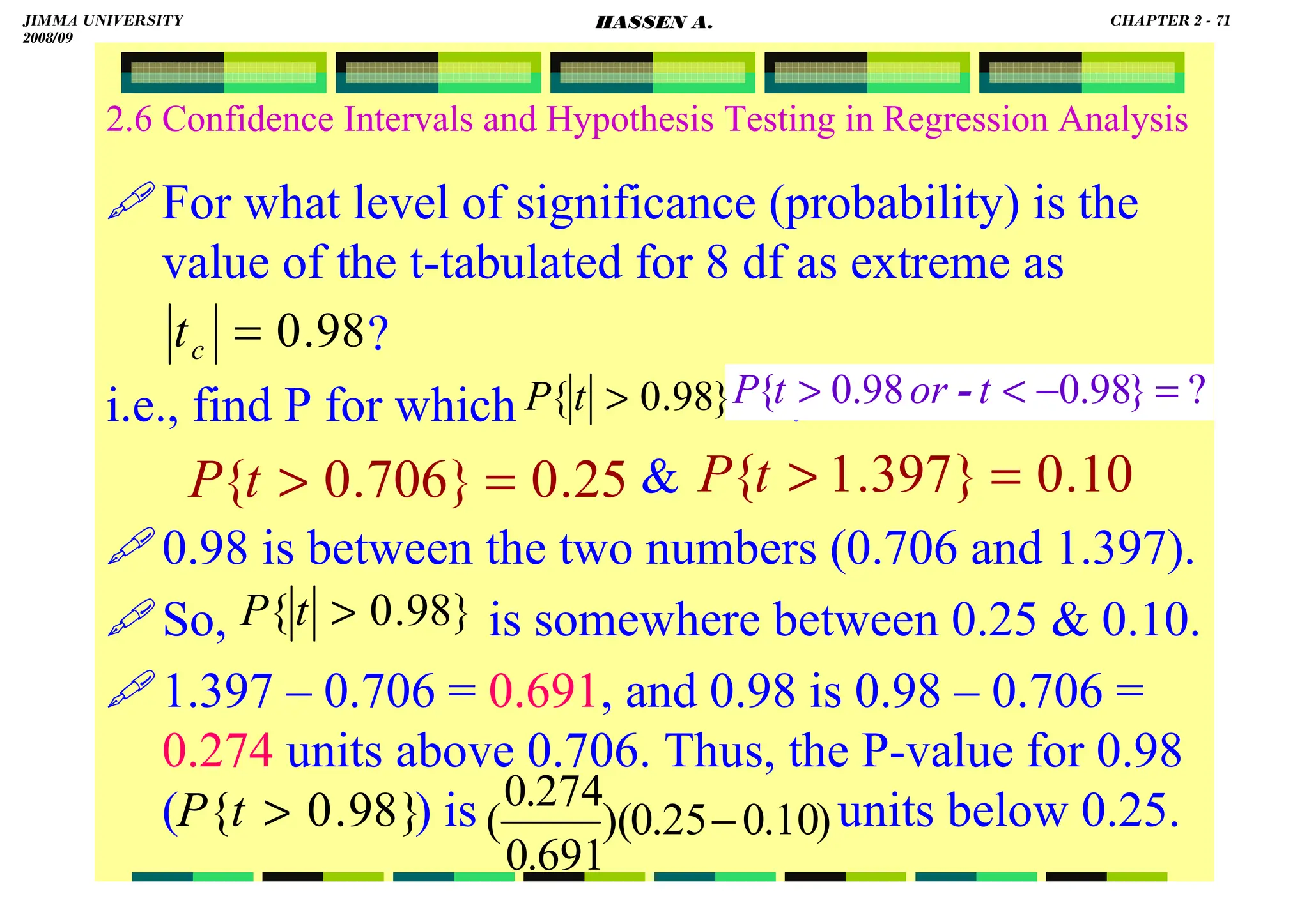
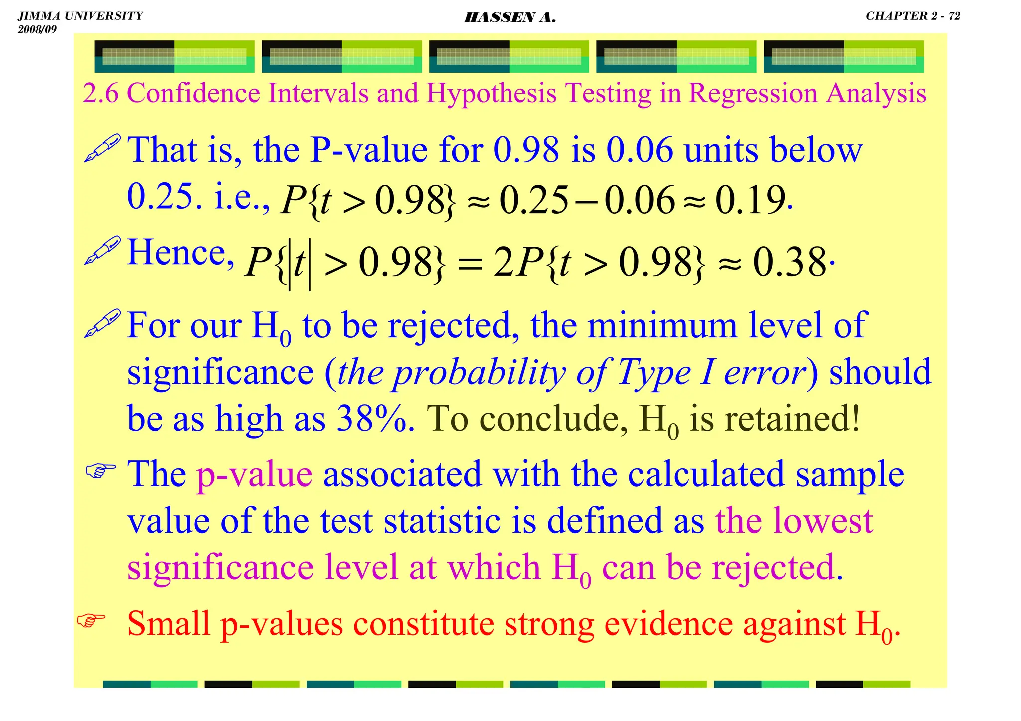
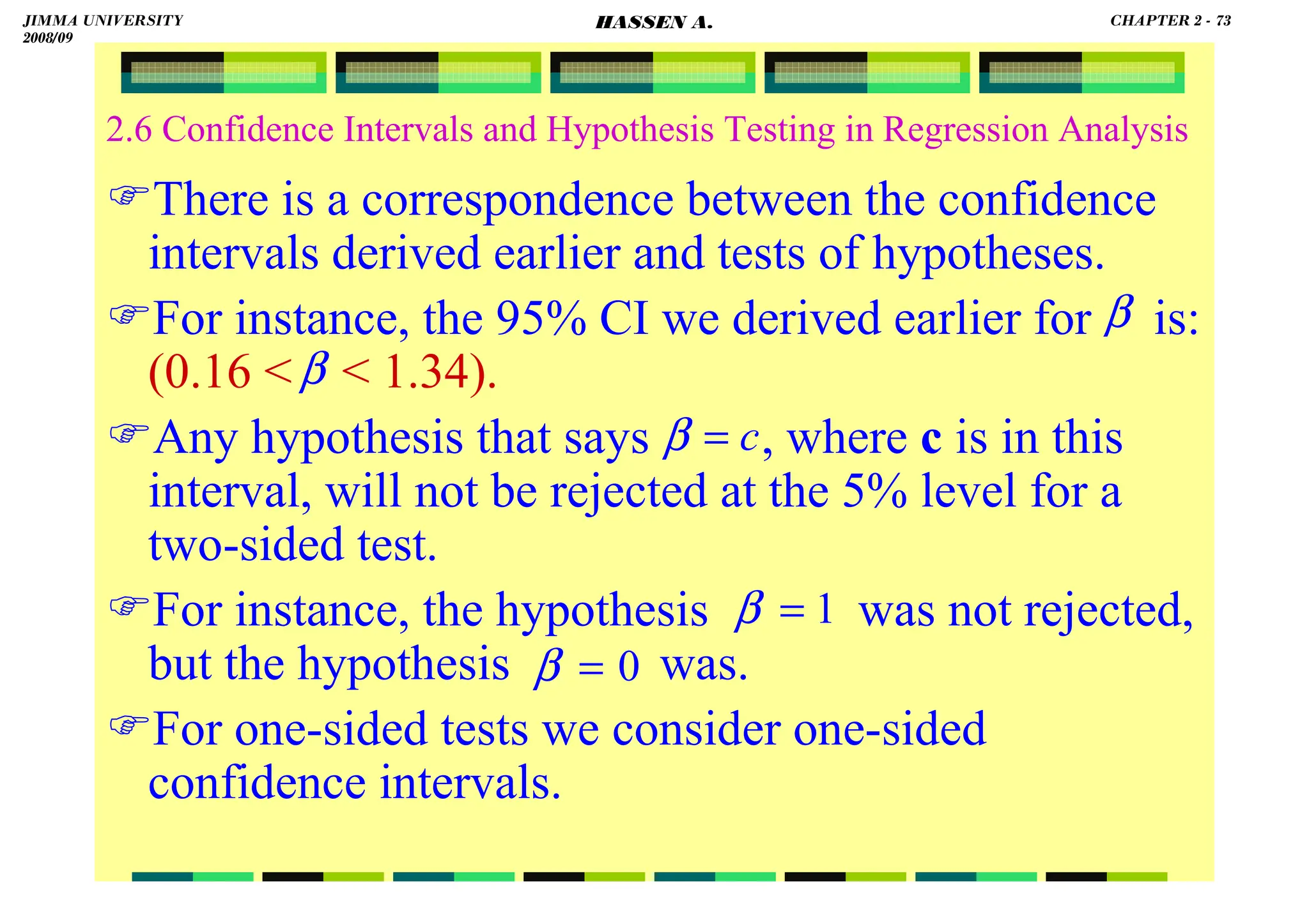
2.6 Confidence Intervals and Hypothesis Testing in Regression Analysis
CI for (continued):
OR
:
r σ
ided CI fo
α)% Two-S
( 2
1
100 −
⇒
2
σ
α
χ
σ
σ
χ
σ
α
α
−
=
−
≤
≤
−
⇒
−
−
−
1
}
ˆ
)
2
(
ˆ
)
2
(
{ 2
2
);
2
/
(
1
2
2
2
2
);
2
/
(
2
n
n
n
n
P
]
ˆ
)
2
(
,
ˆ
)
2
(
[ 2
2
);
2
/
(
1
2
2
2
);
2
/
(
2
−
−
−
−
−
n
n
n
n
α
α χ
σ
χ
σ
]
,
[ 2
2
);
2
/
(
1
2
2
);
2
/
( −
−
− n
n
RSS
RSS
α
α χ
χ
JIMMA UNIVERSITY
2008/09
CHAPTER 2 - 62
HASSEN A.

76. HASSEN ABDA
2.6 Confidence Intervals and Hypothesis Testing in Regression Analysis
Let us continue with our earlier example.
We have:
is estimated by:
Thus,
2
σ
,
3857
.
2
)
ˆ
var( 2
σ
α ≈
,
6
.
3
ˆ =
α ,
75
.
0
ˆ =
β
,
10
=
n
,
0357
.
0
)
ˆ
var( 2
σ
β ≈
,
5181
.
0
2
=
R
83125
.
1
8
65
.
14
2
ˆ
2
2
=
=
−
∑
=
n
e
σ i
65
.
14
2
=
∑ i
e
3532
.
1
83125
.
1
ˆ ≈
=
⇒σ
3688
.
4
)
83125
.
1
(
3857
.
2
)
ˆ
r(
â
v ≈
≈
α
09
.
2
3688
.
4
)
ˆ
(
ˆ ≈
≈
⇒ α
e
s
0654
.
0
)
83125
.
1
(
0357
.
0
)
ˆ
r(
â
v ≈
≈
β
256
.
0
0654
.
0
)
ˆ
(
ˆ ≈
≈
⇒ β
e
s
JIMMA UNIVERSITY
2008/09
CHAPTER 2 - 63
HASSEN A.

77. HASSEN ABDA
2.6 Confidence Intervals and Hypothesis Testing in Regression Analysis
95% CI for :
8195
.
4
6
3 ±
= .
::::
αααα
for
CI
%
95
::::
β
for
CI
%
95
α and β
05
.
0
95
.
0
1 =
⇒
=
− α
α
)
09
.
2
(
306
.
2
)
09
.
2
(
6
3
6
3 8
025
.
0
)
(
)
(t
.
.
±
=
±
:
α
for
CI
95%
⇒
)
256
.
0
(
306
.
2
)
256
.
0
(
75
.
0
75
.
0 8
025
.
0
)
(
)
(t
±
=
±
5903
.
0
75
.
0 ±
=
:
for
CI
95% β
⇒
025
.
0
2
/ =
⇒α
8.4195]
1.2195,
[−
1.3403]
[0.1597,
JIMMA UNIVERSITY
2008/09
CHAPTER 2 - 64
HASSEN A.

78. HASSEN ABDA
2.6 Confidence Intervals and Hypothesis Testing in Regression Analysis
95% CI for :
::::
2
σ
for
CI
%
95
⇒
2
σ
83125
.
1
ˆ 2
=
σ
6.72]
[0.84,
=
:
2
2
;
2
/ −
n
α
χ 5
.
17
2
8
;
025
.
0 =
χ
18
.
2
2
8
;
975
.
0 =
χ
:
2
2
);
2
/
(
1 −
− n
α
χ
]
ˆ
)
2
(
,
ˆ
)
2
(
[ 2
2
);
2
/
(
1
2
2
2
);
2
/
(
2
−
−
−
−
−
n
n
n
n
α
α χ
σ
χ
σ
]
18
.
2
65
.
14
,
5
.
17
65
.
14
[
=
JIMMA UNIVERSITY
2008/09
CHAPTER 2 - 65
HASSEN A.

79. HASSEN ABDA
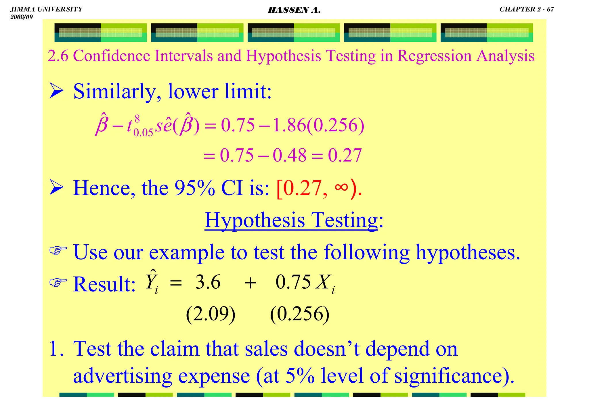
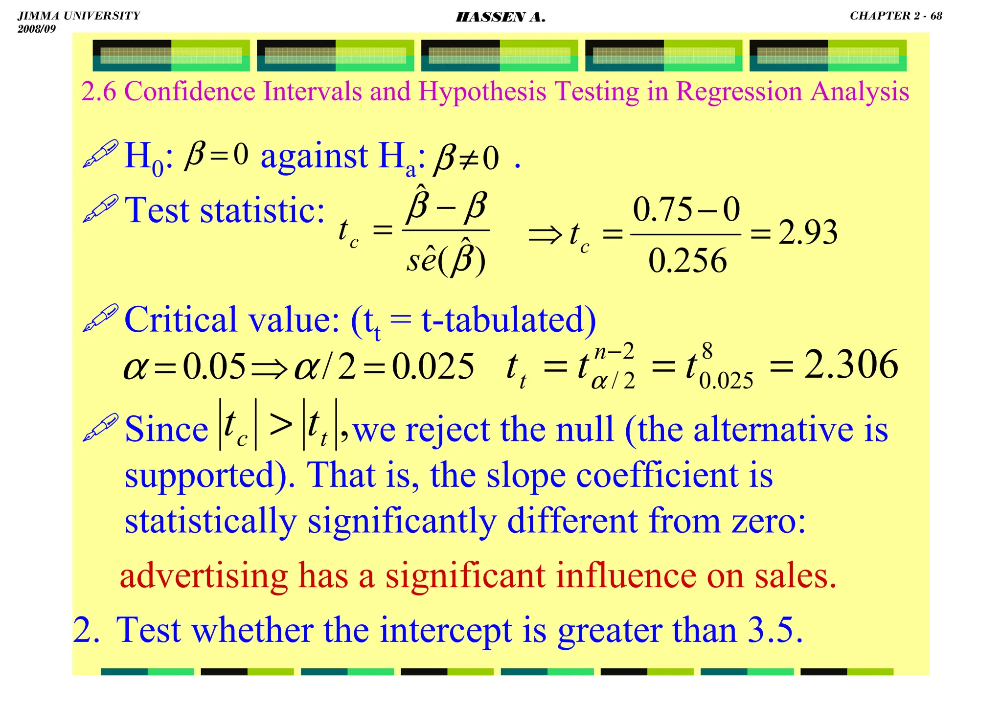
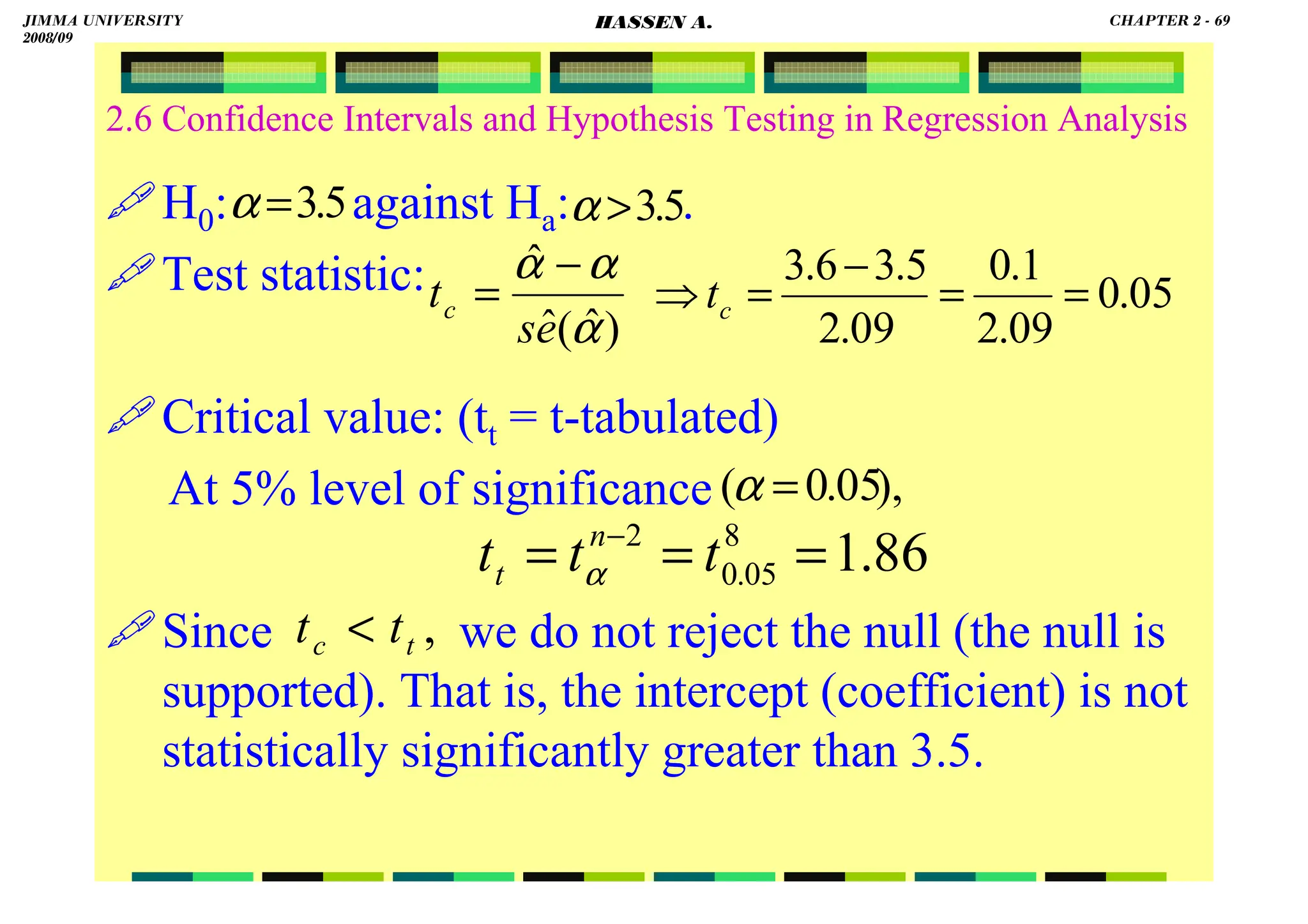
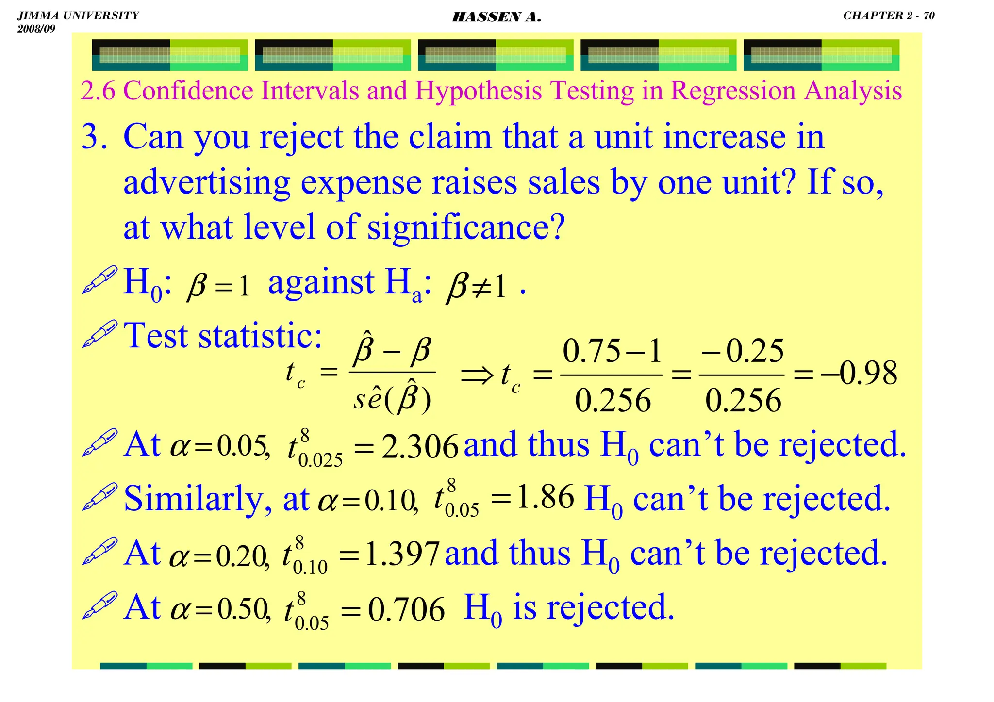
2.6 Confidence Intervals and Hypothesis Testing in Regression Analysis
The confidence intervals we have constructed for
are two-sided intervals.
Sometimes we want either the upper or lower limit
only, in which case we construct one-sided intervals.
For instance, let us construct a one-sided (upper
limit) 95% confidence interval for .
Form the t-table, .
Hence,
The confidence interval is (- ∞, 1.23].
2
, σ
β
α
β
86
.
1
8
05
.
0 =
t
23
.
1
48
.
0
75
.
0
)
256
.
0
(
86
.
1
75
.
0
)
ˆ
(
ˆ
.
ˆ 8
05
.
0
=
+
=
+
=
+ β
β e
s
t
JIMMA UNIVERSITY
2008/09
CHAPTER 2 - 66
HASSEN A.

80. HASSEN ABDA
2.6 Confidence Intervals and Hypothesis Testing in Regression Analysis
Similarly, lower limit:
Hence, the 95% CI is: [0.27, ∞).
Hypothesis Testing:
Use our example to test the following hypotheses.
Result:
1. Test the claim that sales doesn’t depend on
advertising expense (at 5% level of significance).
)
256
.
0
(
)
09
.
2
(
75
.
0
6
.
3
ˆ
i
i X
Y +
=
27
.
0
48
.
0
75
.
0
)
256
.
0
(
86
.
1
75
.
0
)
ˆ
(
ˆ
ˆ 8
05
.
0
=
−
=
−
=
− β
β e
s
t
JIMMA UNIVERSITY
2008/09
CHAPTER 2 - 67
HASSEN A.

81. HASSEN ABDA
2.6 Confidence Intervals and Hypothesis Testing in Regression Analysis
H0: against Ha: .
Test statistic:
Critical value: (tt = t-tabulated)
Since we reject the null (the alternative is
supported). That is, the slope coefficient is
statistically significantly different from zero:
advertising has a significant influence on sales.
2. Test whether the intercept is greater than 3.5.
0
=
β 0
≠
β
025
.
0
2
/
05
.
0 =
⇒
= α
α
)
ˆ
(
ˆ
ˆ
β
β
β
e
s
tc
−
= 93
.
2
256
.
0
0
75
.
0
=
−
=
⇒ c
t
306
.
2
8
025
.
0
2
2
/ =
=
= −
t
t
t n
t α
,
t
c t
t
JIMMA UNIVERSITY
2008/09
CHAPTER 2 - 68
HASSEN A.

82. HASSEN ABDA
2.6 Confidence Intervals and Hypothesis Testing in Regression Analysis
H0: against Ha: .
Test statistic:
Critical value: (tt = t-tabulated)
At 5% level of significance
Since we do not reject the null (the null is
supported). That is, the intercept (coefficient) is not
statistically significantly greater than 3.5.
5
.
3
=
α 5
.
3
α
),
05
.
0
( =
α
)
ˆ
(
ˆ
ˆ
α
α
α
e
s
tc
−
= 05
.
0
09
.
2
1
.
0
09
.
2
5
.
3
6
.
3
=
=
−
=
⇒ c
t
86
.
1
8
05
.
0
2
=
=
= −
t
t
t n
t α
,
t
c t
t
JIMMA UNIVERSITY
2008/09
CHAPTER 2 - 69
HASSEN A.

83. HASSEN ABDA
2.6 Confidence Intervals and Hypothesis Testing in Regression Analysis
3. Can you reject the claim that a unit increase in
advertising expense raises sales by one unit? If so,
at what level of significance?
H0: against Ha: .
Test statistic:
At and thus H0 can’t be rejected.
Similarly, at H0 can’t be rejected.
At and thus H0 can’t be rejected.
At H0 is rejected.
1
=
β 1
≠
β
,
05
.
0
=
α
)
ˆ
(
ˆ
ˆ
β
β
β
e
s
tc
−
= 98
.
0
256
.
0
25
.
0
256
.
0
1
75
.
0
−
=
−
=
−
=
⇒ c
t
306
.
2
8
025
.
0 =
t
,
10
.
0
=
α 86
.
1
8
05
.
0 =
t
,
20
.
0
=
α 397
.
1
8
10
.
0 =
t
,
50
.
0
=
α 706
.
0
8
05
.
0 =
t
JIMMA UNIVERSITY
2008/09
CHAPTER 2 - 70
HASSEN A.

84. HASSEN ABDA
2.6 Confidence Intervals and Hypothesis Testing in Regression Analysis
For what level of significance (probability) is the
value of the t-tabulated for 8 df as extreme as
?
i.e., find P for which .
0.98 is between the two numbers (0.706 and 1.397).
So, is somewhere between 0.25 0.10.
1.397 – 0.706 = 0.691, and 0.98 is 0.98 – 0.706 =
0.274 units above 0.706. Thus, the P-value for 0.98
( ) is units below 0.25.
?
}
98
.
0
98
.
0
{ =
−
t
or
t
P -
}
98
.
0
{
t
P
98
.
0
=
c
t
25
.
0
}
706
.
0
{ =
t
P 10
.
0
}
397
.
1
{ =
t
P
)
10
.
0
25
.
0
)(
691
.
0
274
.
0
( −
}
98
.
0
{
t
P
}
98
.
0
{
t
P
JIMMA UNIVERSITY
2008/09
CHAPTER 2 - 71
HASSEN A.

85. HASSEN ABDA
2.6 Confidence Intervals and Hypothesis Testing in Regression Analysis
That is, the P-value for 0.98 is 0.06 units below
0.25. i.e., .
Hence, .
For our H0 to be rejected, the minimum level of
significance (the probability of Type I error) should
be as high as 38%. To conclude, H0 is retained!
The p-value associated with the calculated sample
value of the test statistic is defined as the lowest
significance level at which H0 can be rejected.
Small p-values constitute strong evidence against H0.
38
.
0
}
98
.
0
{
2
}
98
.
0
{ ≈
=
t
P
t
P
19
.
0
06
.
0
25
.
0
}
98
.
0
{ ≈
−
≈
t
P
JIMMA UNIVERSITY
2008/09
CHAPTER 2 - 72
HASSEN A.

86. HASSEN ABDA
2.6 Confidence Intervals and Hypothesis Testing in Regression Analysis
There is a correspondence between the confidence
intervals derived earlier and tests of hypotheses.
For instance, the 95% CI we derived earlier for is:
(0.16 1.34).
Any hypothesis that says , where c is in this
interval, will not be rejected at the 5% level for a
two-sided test.
For instance, the hypothesis was not rejected,
but the hypothesis was.
For one-sided tests we consider one-sided
confidence intervals.
β
β
c
=
β
1
=
β
0
=
β
JIMMA UNIVERSITY
2008/09
CHAPTER 2 - 73
HASSEN A.

87. HASSEN ABDA
2.7 Prediction with the Simple Linear Regression
The estimated regression equation is used
for predicting the value (or the average value) of Y
for given values of X.
Let X0 be the given value of X. Then we predict the
corresponding value YP of Y by:
The true value YP is given by:
Hence the prediction error is:
is an unbiased predictor of Y. (BLUP!)
i
i X
Y β
α ˆ
ˆ
ˆ +
=
0
ˆ
ˆ
ˆ X
YP β
α +
=
P
P X
Y ε
β
α +
+
= 0
P
P
P X
Y
Y ε
β
β
α
α −
−
+
−
=
− 0
)
ˆ
(
)
ˆ
(
ˆ
)
(
)
ˆ
(
)
ˆ
(
)
ˆ
( 0 P
P
P E
X
E
E
Y
Y
E ε
β
β
α
α −
−
+
−
=
−
0
ˆ
ˆ
ˆ X
YP β
α +
=
0
)
ˆ
( =
−
⇒ P
P Y
Y
E
JIMMA UNIVERSITY
2008/09
CHAPTER 2 - 74
HASSEN A.

88. HASSEN ABDA
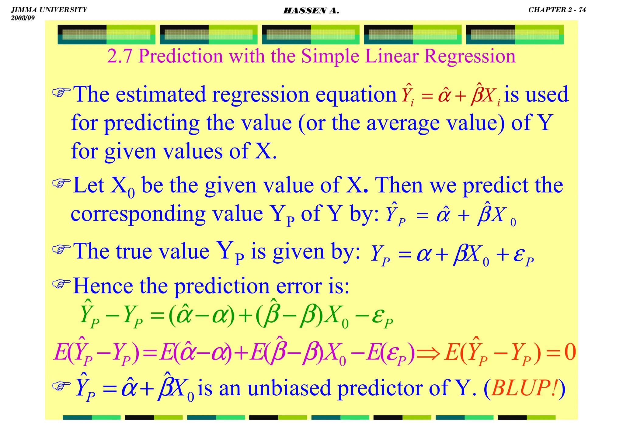
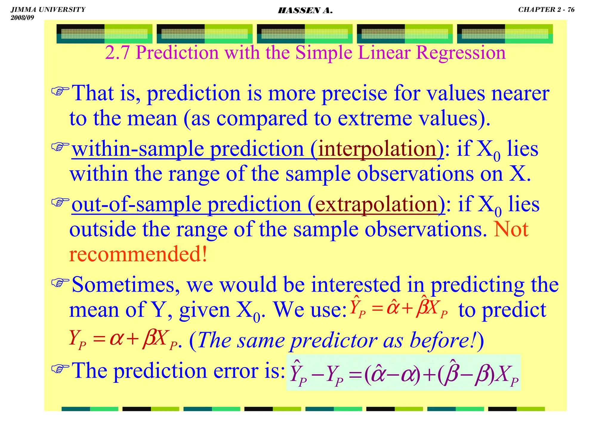
2.7 Prediction with the Simple Linear Regression
The variance of the prediction error is:
Thus, the variance increases the farther away the
value of X0 is from , the mean of the observations
on the basis of which have been computed.
)
var(
)
ˆ
,
ˆ
cov(
2
)
ˆ
var(
)
ˆ
var(
)
ˆ
var(
0
2
0
P
P
P
X
X
Y
Y
ε
β
β
α
α
β
β
α
α
+
−
−
+
−
+
−
=
−
2
2
2
0
2
2
0
2
2
2
2
2
)
ˆ
var( σ
σ
σ
σ +
−
+
=
−
∑
∑
∑
∑
i
i
i
i
P
P
x
X
X
x
X
x
n
X
Y
Y
]
)
(
1
1
[
)
ˆ
var( 2
2
0
2
∑
−
+
+
=
−
i
P
P
x
X
X
n
Y
Y σ
X
β
α ˆ
ˆ
JIMMA UNIVERSITY
2008/09
CHAPTER 2 - 75
HASSEN A.

89. HASSEN ABDA
2.7 Prediction with the Simple Linear Regression
That is, prediction is more precise for values nearer
to the mean (as compared to extreme values).
within-sample prediction (interpolation): if X0 lies
within the range of the sample observations on X.
out-of-sample prediction (extrapolation): if X0 lies
outside the range of the sample observations. Not
recommended!
Sometimes, we would be interested in predicting the
mean of Y, given X0. We use: to predict
. (The same predictor as before!)
The prediction error is:
P
P X
Y β
α ˆ
ˆ
ˆ +
=
P
P X
Y β
α +
=
P
P
P X
Y
Y )
ˆ
(
)
ˆ
(
ˆ β
β
α
α −
+
−
=
−
JIMMA UNIVERSITY
2008/09
CHAPTER 2 - 76
HASSEN A.

90. HASSEN ABDA
2.7 Prediction with the Simple Linear Regression
The variance of the prediction error is:
Again, the variance increases the farther away the
value of X0 is from .
The variance (the standard error) of the prediction
error is smaller in this case (of predicting the
average value of Y, given X) than that of predicting
a value of Y, given X.
)
ˆ
,
ˆ
cov(
2
)
ˆ
var(
)
ˆ
var(
)
ˆ
var( 0
2
0 β
β
α
α
β
β
α
α −
−
+
−
+
−
=
− X
X
Y
Y P
P
]
)
(
1
[
)
ˆ
var( 2
2
0
2
∑
−
+
=
−
⇒
i
P
P
x
X
X
n
Y
Y σ
X
JIMMA UNIVERSITY
2008/09
CHAPTER 2 - 77
HASSEN A.

91. HASSEN ABDA
78
2.7 Prediction with the Simple Linear Regression
Predict (a) the value of sales, and (b) the average
value of sales, for a firm with an advertising expense
of six hundred Birr.
a. From , at Xi = 6,
Point prediction:
[Sales value | advertising of 600 Birr] = 8,100 Birr.
Interval prediction: 95% CI:
]
)
(
1
1
[
ˆ
)
ˆ
(
ˆ 2
2
0
2
*
∑
−
+
+
=
i
P
x
X
X
n
Y
e
s σ
i
i X
Y 75
.
0
6
.
3
ˆ +
=
1
.
8
)
6
(
75
.
0
6
.
3
ˆ =
+
=
i
Y
28
)
8
6
(
10
1
1
35
.
1
)
ˆ
(
ˆ
2
* −
+
+
=
⇒ P
Y
e
s
508
.
1
)
115
.
1
(
35
.
1 =
=
306
.
2
8
025
.
0 =
t
JIMMA UNIVERSITY
2008/09
CHAPTER 2 - 78
HASSEN A.

92. HASSEN ABDA
79
2.7 Prediction with the Simple Linear Regression
Hence,
b. From , at Xi = 6,
Point prediction:
[Average sales | advertising of 600 Birr] = 8,100 Birr.
Interval prediction: 95% CI:
]
)
(
1
[
ˆ
)
ˆ
(
ˆ 2
2
0
2
*
∑
−
+
=
i
P
x
X
X
n
Y
e
s σ
1
.
8
)
6
(
75
.
0
6
.
3
ˆ =
+
=
i
Y
28
)
8
6
(
10
1
35
.
1
)
ˆ
(
2
* −
+
=
⇒ P
Y
se
)
508
.
1
)(
306
.
2
(
1
.
8
%
95 ±
:
CI
]
58
.
11
,
62
.
4
[
i
X
Yi
75
.
0
6
.
3
ˆ +
=
667
.
0
)
493
.
0
(
35
.
1
)
ˆ
(
ˆ *
=
=
⇒ P
Y
e
s
)
667
.
0
)(
306
.
2
(
1
.
8
%
95 ±
:
CI ]
64
.
9
,
56
.
6
[
JIMMA UNIVERSITY
2008/09
CHAPTER 2 - 79
HASSEN A.

93. HASSEN ABDA
Notes on interpreting the coefficient of X in simple linear regression
1.
2.
ε
β
α +
+
= X
Y slope
dX
dY
dX
dY =
=
⇒
=
⇒ β
β.
ε
β
α +
+
= X
e
Y ε
β
α +
+
=
⇒ X
Y
ln
X.
in
change
unit
a
from
resulting
Y
in
change
(AVERAGE)
the
is
β
dX
dY
Y
dX
Y
d .
.
1
.
)
(ln β
β =
⇒
=
⇒
X.
in
change
unit
a
from
ting
-
resul
Y
in
change
percentage
(AVERAGE)
the
is
100)
(
β ×
)
100
(
. ×
=
⇒ dX
Y
in
∆
%age β
X
in
Absolute
Y
in
∆
Relative
∆
=
=
⇒
dX
Y
dY )
(
β
dX
Y
in
∆
%age
=
×
=
×
⇒
dX
Y
dY 100
)
(
)
100
(
β
JIMMA UNIVERSITY
2008/09
CHAPTER 2 - 80
HASSEN A.

94. HASSEN ABDA
81
Notes on interpreting the coefficient of X in simple linear regression
3.
4. ε
β
e
AX
Y = A
X
Y ln
;
)
(ln
ln =
+
+
=
⇒ α
ε
β
α
X
in
age
Y
in
age
X
dX
Y
dY
X
d
Y
d
∆
∆
=
=
=
⇒
%
%
/
/
)
(ln
)
(ln
β
Elasticity
=
X.
in
change
percentage
a
from
resulting
Y
in
change
(AVERAGE)
the
is
0.01)
(
β ×
X.
in
change
percentage
a
from
resulting
Y
in
change
percentage
(AVERAGE)
the
is
β
E
AX
eY β
= ;
ln ε
β
α +
+
=
⇒ X
Y
X
in
Relative
Y
in
Absolute
∆
∆
=
=
=
⇒
dX
X
dY
X
d
dY
)
1
(
)
(ln
β
)
ln(
)
ln( E
A =
= ε
α
)
).(%
01
.
0
( X
in
age
dY ∆
=
⇒ β
)
100
.(
100
×
=
⇒
X
dX
dY
β
JIMMA UNIVERSITY
2008/09
CHAPTER 2 - 81
HASSEN A.

95. HASSEN ABDA
STATA SESSION
JIMMA UNIVERSITY
2008/09
CHAPTER 2 - 82
HASSEN A.

96. .
CHAPTER THREE
THE MULTIPLE LINEAR REGRESSION
CHAPTER THREE
THE MULTIPLE LINEAR REGRESSION
3.1 Introduction: The Multiple Linear Regression
3.2 Assumptions of the Multiple Linear Regression
3.3 Estimation: The Method of OLS
3.4 Properties of OLS Estimators
3.5 Partial Correlations and Coefficients of
Multiple Determination
3.6 Statistical Inferences in Multiple Linear
Regression
3.7 Prediction with Multiple Linear Regression
JIMMA UNIVERSITY
2008/09
CHAPTER 3 - 1
HASSEN A.

97. .
3.1 Introduction: The Multiple Linear Regression
i
Ki
K
i
i
i X
X
X
Y ε
β
β
β
β +
+
•
•
•
+
+
+
= 2
2
1
1
0
Relationship between a dependent two or more
independent variables is a linear function
Population
Y-intercept
Population slopes
Dependent (Response)
variable (for sample)
Independent (Explanatory)
variables (for sample)
Random
Error
i
Ki
K
i
i
i e
X
X
X
Y +
+
•
•
•
+
+
+
= β
β
β
β ˆ
ˆ
ˆ
ˆ
2
2
1
1
0
Residual
JIMMA UNIVERSITY
2008/09
CHAPTER 3 - 2
HASSEN A.

98. .
3.1 Introduction: The Multiple Linear Regression
3.1 Introduction: The Multiple Linear Regression
) What changes as we move from simple to
multiple regression?
1. Potentially more explanatory power with more
variables;
2. The ability to control for other variables; (and
the interaction of the various explanatory
variables: correlations and multicollinearity);
3. Harder to visualize drawing a line through
three or more (n)-dimensional space.
4. The R2 is no longer simply the square of the
correlation coefficient between Y and X.
JIMMA UNIVERSITY
2008/09
CHAPTER 3 - 3
HASSEN A.

99. .
3.1 Introduction: The Multiple Linear Regression
)Slope ( ):
Ceteris paribus, Y changes by for every 1 unit
change in , on average.
)Y-Intercept ( ):
The average value of Y when all s are zero.
(may not be meaningful all the time)
)A multiple linear regression model is defined to
be linear in the regression parameters rather
than in the explanatory variables.
)Thus, the definition of multiple linear regression
includes polynomial regression.
e.g.
j
β
j
β
j
X
0
β
j
X
i
i
i
i
i
i
i X
X
X
X
X
Y ε
β
β
β
β
β +
+
+
+
+
= 2
1
4
2
1
3
2
2
1
1
0
JIMMA UNIVERSITY
2008/09
CHAPTER 3 - 4
HASSEN A.

100. .
3.2 Assumptions of the Multiple Linear Regression
3.2 Assumptions of the Multiple Linear Regression
)Assumptions 1 – 7 in Chapter Two.
1. E(ɛi|Xji) = 0. (for all i = 1, 2, …, n; j = 1, …, K)
2. var(ɛi|Xji) = σ2. (i ≠ s) (Homoscedastic errors)
3. cov(ɛi,ɛs|Xji,Xjs) = 0. (i ≠ s) (No autocorrelation)
4. cov(ɛi,Xji) = 0. Errors are orthogonal to the Xs.
5. Xj is non-stochastic, and must assume different
values.
6. n K+1. (Number of observations number of
parameters to be estimated). Number of
parameters is K+1 in this case ( β0, β1, …, βK )
7. ɛi ~N(0, σ2). Normally distributed errors.
JIMMA UNIVERSITY
2008/09
CHAPTER 3 - 5
HASSEN A.

101. .
3.2 Assumptions of the Multiple Linear Regression
3.2 Assumptions of the Multiple Linear Regression
) Additional Assumption:
8. No perfect multicollinearity: That is, no exact
linear relation exists between any subset of
explanatory variables.
) In the presence of perfect (deterministic) linear
relationship between/among any set of the Xjs,
the impact of a single variable ( ) cannot be
identified.
) More on multicollinearity in a later chapter!
j
β
JIMMA UNIVERSITY
2008/09
CHAPTER 3 - 6
HASSEN A.

102. .
3.3 Estimation: The Method of OLS
3.3 Estimation: The Method of OLS
The Case of Two Regressors (X
The Case of Two Regressors (X1
1 and X
and X2
2)
)
) Minimize the RSS with respect to .
)
ˆ
(
ˆ
ˆ Y
Y
Y
Y
Y
Y
Y
Y
Y
Y
e i
i
i
i
i
i
i −
−
−
=
−
+
−
=
−
=
2
1
ˆ
ˆ β
β
i
i
i X
X
Y 2
2
1
1
0
ˆ
ˆ
ˆ
ˆ β
β
β +
+
=
i
i
i X
X
Y 2
2
1
1
0
ˆ
ˆ
ˆ
ˆ β
β
β +
+
=
∑
∑ −
−
=
= 2
2
2
1
1
2
)
ˆ
ˆ
( i
i
i
i x
x
y
e
RSS β
β
0
2 =
−
⇒ ∑ ji
i x
e
2
,
1
;
0
)
(
)
ˆ
ˆ
(
2
ˆ
)
(
2
2
1
1 =
=
−
−
−
=
∂
∂
∑ j
x
x
x
y
RSS
ji
i
i
i
j
β
β
β
i
i
i x
x
y 2
2
1
1
ˆ
ˆ
ˆ β
β +
=
i
i
i y
y
e ˆ
−
=
⇒
0
)
(
)
ˆ
ˆ
(
.
1 1
2
2
1
1 =
−
−
∑ i
i
i
i x
x
x
y β
β
∑
∑
∑ +
=
⇒ i
i
i
i
i x
x
x
x
y 2
1
2
2
1
1
1
ˆ
ˆ β
β
0
)
(
)
ˆ
ˆ
(
.
2 2
2
2
1
1 =
−
−
∑ i
i
i
i x
x
x
y β
β
∑
∑
∑ +
=
⇒ 2
2
2
2
1
1
2
ˆ
ˆ
i
i
i
i
i x
x
x
x
y β
β
JIMMA UNIVERSITY
2008/09
CHAPTER 3 - 7
HASSEN A.

103. .
3.3 Estimation: The Method of OLS
3.3 Estimation: The Method of OLS
Solve for the coefficients:
Determinant:
To find , substitute the first column of A by
elements of F, then find |A1|, and finally find .
⎟
⎟
⎠
⎞
⎜
⎜
⎝
⎛
⎥
⎥
⎦
⎤
⎢
⎢
⎣
⎡
=
⎟
⎟
⎠
⎞
⎜
⎜
⎝
⎛
⇒
∑
∑
∑
∑
∑
∑
2
1
2
2i
1i
2i
2i
1i
2
1i
2i
i
1i
i
β
β
x
x
x
x
x
x
x
y
x
y
ˆ
ˆ
2
2
1
2
2
2
1
2
2
2
1
2
1
2
1
)
(∑
∑
∑
∑
∑
∑
∑ −
=
= i
i
i
i
i
i
i
i
i
i
x
x
x
x
x
x
x
x
x
x
A
1
β̂
=
F
A
A1
)
)(
(
)
)(
( 2
2
1
2
2
1
2
2
2
2
1
1
1 ∑
∑
∑
∑
∑
∑
∑
∑ −
=
= i
i
i
i
i
i
i
i
i
i
i
i
i
i
x
y
x
x
x
x
y
x
x
y
x
x
x
y
A
2
2
1
2
2
2
1
2
2
1
2
2
1
1
1
)
(
)
)(
(
)
)(
(
)
)(
(
ˆ
∑
∑
∑
∑
∑
∑
∑
−
−
=
=
i
i
i
i
i
i
i
i
i
i
i
x
x
x
x
x
y
x
x
x
x
y
A
A
β
•
A β̂
JIMMA UNIVERSITY
2008/09
CHAPTER 3 - 8
HASSEN A.

104. .
3.3 Estimation: The Method of OLS
3.3 Estimation: The Method of OLS
Similarly, to find , substitute the second column
of A by elements of F, then find |A2|, and finally
find .
2
β̂
A
A2
)
)(
(
)
)(
( 1
2
1
2
1
2
2
2
1
1
2
1
2 ∑
∑
∑
∑
∑
∑
∑
∑ −
=
= i
i
i
i
i
i
i
i
i
i
i
i
i
i
x
y
x
x
x
x
y
x
y
x
x
x
y
x
A
2
2
1
2
2
2
1
1
2
1
2
1
2
2
2
)
(
)
)(
(
)
)(
(
)
)(
(
ˆ
∑
∑
∑
∑
∑
∑
∑
−
−
=
=
i
i
i
i
i
i
i
i
i
i
i
x
x
x
x
x
y
x
x
x
x
y
A
A
β
2
2
1
1
0
ˆ
ˆ
ˆ X
X
Y
β β
β −
−
=
JIMMA UNIVERSITY
2008/09
CHAPTER 3 - 9
HASSEN A.

105. .
The Case of
The Case of K
K Explanatory Variables
Explanatory Variables
) The number of parameters to be estimated:
K+1 ( ).
n
Kn
K
n
n
n
K
K
K
K
K
K
e
X
X
X
Y
e
X
X
X
Y
e
X
X
X
Y
e
X
X
X
Y
+
+
+
+
+
=
+
+
+
+
+
=
+
+
+
+
+
=
+
+
+
+
+
=
β
β
β
β
β
β
β
β
β
β
β
β
β
β
β
β
ˆ
ˆ
ˆ
ˆ
ˆ
ˆ
ˆ
ˆ
ˆ
ˆ
ˆ
ˆ
ˆ
ˆ
ˆ
ˆ
2
2
1
1
0
3
3
23
2
13
1
0
3
2
2
22
2
12
1
0
2
1
1
21
2
11
1
0
1
…
…
…
…
K
3.3 Estimation: The Method of OLS
3.3 Estimation: The Method of OLS
β
β
β
β ,
,
, 2
,
1
0 …
JIMMA UNIVERSITY
2008/09
CHAPTER 3 - 10
HASSEN A.

106. .
3.3 Estimation: The Method of OLS
3.3 Estimation: The Method of OLS
.
⎥
⎥
⎥
⎥
⎥
⎥
⎦
⎤
⎢
⎢
⎢
⎢
⎢
⎢
⎣
⎡
+
⎥
⎥
⎥
⎥
⎥
⎥
⎦
⎤
⎢
⎢
⎢
⎢
⎢
⎢
⎣
⎡
•
⎥
⎥
⎥
⎥
⎥
⎥
⎦
⎤
⎢
⎢
⎢
⎢
⎢
⎢
⎣
⎡
=
⎥
⎥
⎥
⎥
⎥
⎥
⎦
⎤
⎢
⎢
⎢
⎢
⎢
⎢
⎣
⎡
n
3
2
1
K
2
1
0
Kn
K3
K2
K1
3n
33
32
31
2n
23
22
21
1n
13
12
11
n
3
2
1
e
e
e
e
β
β
β
β
X
X
X
X
X
X
X
X
X
X
X
X
X
X
X
X
1
1
1
1
Y
Y
Y
Y
…
…
…
…
ˆ
ˆ
ˆ
ˆ
1
×
n )
1
( +
× K
n 1
×
n
1
)
1
( ×
+
K
e
X
Y +
= β
ˆ
JIMMA UNIVERSITY
2008/09
CHAPTER 3 - 11
HASSEN A.

107. .
3.3 Estimation: The Method of OLS
3.3 Estimation: The Method of OLS
.
⎥
⎥
⎥
⎥
⎥
⎥
⎦
⎤
⎢
⎢
⎢
⎢
⎢
⎢
⎣
⎡
⎥
⎥
⎥
⎥
⎥
⎥
⎦
⎤
⎢
⎢
⎢
⎢
⎢
⎢
⎣
⎡
−
⎥
⎥
⎥
⎥
⎥
⎥
⎦
⎤
⎢
⎢
⎢
⎢
⎢
⎢
⎣
⎡
=
⎥
⎥
⎥
⎥
⎥
⎥
⎦
⎤
⎢
⎢
⎢
⎢
⎢
⎢
⎣
⎡
K
2
1
0
Kn
K3
K2
K1
3n
33
32
31
2n
23
22
21
1n
13
12
11
n
3
2
1
n
3
2
1
β
β
β
β
*
X
X
X
X
X
X
X
X
X
X
X
X
X
X
X
X
1
1
1
1
Y
Y
Y
Y
e
e
e
e
ˆ
ˆ
ˆ
ˆ
…
…
…
…
β̂
X
Y
e −
=
JIMMA UNIVERSITY
2008/09
CHAPTER 3 - 12
HASSEN A.

108. .
3.3 Estimation: The Method of OLS
3.3 Estimation: The Method of OLS
0
)
ˆ
(
)
(
:
.
.
. =
∂
∂
β
RSS
C
O
F
( )
⎟
⎟
⎟
⎟
⎟
⎠
⎞
⎜
⎜
⎜
⎜
⎜
⎝
⎛
=
+
+
+
=
=∑
n
2
1
n
2
1
2
n
2
2
2
1
2
i
e
e
e
.
e
e
e
e
...
e
e
e
RSS …
)
β
X
(Y
)'
β
X
(Y ˆ
ˆ −
−
=
RSS
e
e'
=
⇒RSS
Y
X'
'
β
)'
β
X
(Y'
β
X
Y'
costant,
a
is
β
X
Y'
Since ˆ
ˆ
ˆ
ˆ =
=
β
X
X'
'
β
Y
X'
'
β
Y
Y' ˆ
)
(
ˆ
ˆ
2 +
−
=
⇒ RSS
β
X
X'
'
β
Y
X'
'
β
β
X
Y'
Y
Y' ˆ
ˆ
ˆ
ˆ +
−
−
=
0
β
X
X'
Y
X'
β
=
+
−
=
∂
∂
⇒ ˆ
2
2
)
ˆ
(
)
(RSS
0
β
X
Y
X' =
−
−
⇒ )
ˆ
(
2
JIMMA UNIVERSITY
2008/09
CHAPTER 3 - 13
HASSEN A.

109. .
3.3 Estimation: The Method of OLS
3.3 Estimation: The Method of OLS
.
)
,...,
2
,
1
(
.
0
.
2 K
j
X
e ji
i =
=
∑
0
.
1 =
∑ i
e
⎟
⎟
⎟
⎟
⎟
⎠
⎞
⎜
⎜
⎜
⎜
⎜
⎝
⎛
=
⎟
⎟
⎟
⎟
⎟
⎠
⎞
⎜
⎜
⎜
⎜
⎜
⎝
⎛
⎥
⎥
⎥
⎥
⎥
⎦
⎤
⎢
⎢
⎢
⎢
⎢
⎣
⎡
⇒
0
0
0
.
1
1
1
2
1
2
1
2
1
22
12
21
11
…
…
…
…
n
Kn
K
K
n
n
e
e
e
X
X
X
X
X
X
X
X
X
Y
X'
X
X'
β 1
−
= )
(
ˆ
Y
X'
β
X
X' =
⇒ ˆ
0
e
X' =
⇒
0
)
β
X
(Y
X'
e
X' =
−
= ˆ
JIMMA UNIVERSITY
2008/09
CHAPTER 3 - 14
HASSEN A.

110. .
3.3 Estimation: The Method of OLS
3.3 Estimation: The Method of OLS
⎥
⎥
⎥
⎥
⎦
⎤
⎢
⎢
⎢
⎢
⎣
⎡
⎥
⎥
⎥
⎥
⎦
⎤
⎢
⎢
⎢
⎢
⎣
⎡
=
n
K
K
n
Kn
K
K
n
X
X
X
X
X
X
X
X
X
X
X
X
2
2
1
1
12
11
2
1
1
12
11
1
1
1
.
1
1
1
…
…
…
…
…
…
X
X/
⎥
⎥
⎥
⎥
⎥
⎦
⎤
⎢
⎢
⎢
⎢
⎢
⎣
⎡
=
⇒
∑
∑
∑
∑
∑
∑
∑
∑
2
1
1
2
1
1
1
K
K
K
K
K X
X
X
X
X
X
X
X
X
X
n
…
…
…
X
X/
⎟
⎟
⎟
⎟
⎟
⎠
⎞
⎜
⎜
⎜
⎜
⎜
⎝
⎛
=
K
β
β
β
ˆ
ˆ
ˆ
ˆ 1
0
β
⎥
⎥
⎥
⎥
⎦
⎤
⎢
⎢
⎢
⎢
⎣
⎡
⎥
⎥
⎥
⎥
⎦
⎤
⎢
⎢
⎢
⎢
⎣
⎡
=
n
Kn
K
K
n
Y
Y
Y
X
X
X
X
X
X
…
…
…
2
1
2
1
1
12
11
1
1
1
Y
X /
⎥
⎥
⎥
⎥
⎦
⎤
⎢
⎢
⎢
⎢
⎣
⎡
=
⇒
∑
∑
∑
K
YX
YX
Y
1
Y
X/
JIMMA UNIVERSITY
2008/09
CHAPTER 3 - 15
HASSEN A.

111. .
3.3 Estimation: The Method of OLS
3.3 Estimation: The Method of OLS
.
⎟
⎟
⎟
⎟
⎟
⎟
⎟
⎠
⎞
⎜
⎜
⎜
⎜
⎜
⎜
⎜
⎝
⎛
⎥
⎥
⎥
⎥
⎥
⎥
⎦
⎤
⎢
⎢
⎢
⎢
⎢
⎢
⎣
⎡
=
⎟
⎟
⎟
⎟
⎟
⎟
⎟
⎠
⎞
⎜
⎜
⎜
⎜
⎜
⎜
⎜
⎝
⎛
∑
∑
∑
∑
∑
∑
∑
∑
∑
∑
∑
∑
∑
∑
∑
∑
∑
∑
∑
K
K
K
K
K
K
K
K
K
YX
YX
YX
Y
X
X
X
X
X
X
X
X
X
X
X
X
X
X
X
X
X
X
X
X
X
n
β
β
β
β
…
…
…
…
2
1
2
2
1
2
2
2
1
2
2
1
2
1
2
1
1
2
1
2
1
0
ˆ
ˆ
ˆ
ˆ
1
-
Y)
(X'
X)
(X'
β 1
−
=
ˆ
1
1 ×
+ )
(K )
1
(
1 +
×
+ K
)
(K 1
1×
+ )
(K
JIMMA UNIVERSITY
2008/09
CHAPTER 3 - 16
HASSEN A.

112. .
3.4 Properties of OLS Estimators
)Given the assumptions of the classical linear
regression model (in Section 3.2), the OLS
estimators of the partial regression coefficients
are BLUE: linear, unbiased and have minimum
variance in the class of all linear unbiased
estimators – the Gauss-Markov Theorem.
)In cases where the small-sample desirable
properties (BLUE) may not be found, we look for
asymptotic (or large-sample) properties, like
consistency and asymptotic normality (CLT).
)The OLS estimators are consistent:
0
)
ˆ
(
lim =
−
∞
→
β
β
n
p ˆ
lim var( ) 0
n→∞
=
β
JIMMA UNIVERSITY
2008/09
CHAPTER 3 - 17
HASSEN A.

113. .
)In the multiple regression equation with 2
regressors (X1 and X2), , we
can talk of:
¾the joint effect of X1 and X2 on Y, and
¾the partial effect of X1 or X2 on Y.
)The partial effect of X1 is measured by and the
partial effect of X2 is measured by .
)Partial effect: holding the other variable constant
or after eliminating the effect of the other variable.
)Thus, is interpreted as measuring the effect of
X1 on Y after eliminating the effect of X2 on X1.
1
β̂
2
β̂
1
β̂
i
i
i
i e
X
X
Y +
+
+
= 2
2
1
1
0
ˆ
ˆ
ˆ β
β
β
3.5 Partial Correlations and Coefficients of Determination
JIMMA UNIVERSITY
2008/09
CHAPTER 3 - 18
HASSEN A.

114. .
)Similarly, measures the effect of X2 on Y after
eliminating the effect of X1 on X2.
)Thus, we can derive the estimator of in two
steps (by estimating two separate regressions):
)Step 1: Regress X1 on X2 (an auxiliary regression
to eliminate the effect of X2 from X1). Let the
regression equation be:
Or, in deviation form:
Then,
) is part of X1 which is free from the influence
of X2.
2
β̂
3.5 Partial Correlations and Coefficients of Determination
1
β̂ 1
β
12
2
12
1 e
X
b
a
X +
+
=
12
e
∑
∑
= 2
2
2
1
12
x
x
x
b
12
2
12
1 e
x
b
x +
=
JIMMA UNIVERSITY
2008/09
CHAPTER 3 - 19
HASSEN A.

115. .
)Step 2: Regress Y on e12 (residualized X1). Let the
regression equation be: in
deviation form.
Then,
) is the same as in the multiple regression,
)Proof: (You may skip the proof!)
v
e
b
y ye
3.5 Partial Correlations and Coefficients of Determination
+
= 12
ye
b
∑
∑
= 2
12
12
e
ye
bye
.
ˆ
ˆ
2
2
1
1 e
x
x
y +
+
= β
β
1
β̂
∑
∑
∑
∑
−
−
=
= 2
2
12
1
2
12
1
2
12
12
)
(
)
(
x
b
x
x
b
x
y
e
ye
bye
∑
∑
∑
∑
∑
−
+
−
=
⇒
2
1
12
2
2
2
12
2
1
2
12
1
2 x
x
b
x
b
x
yx
b
yx
bye
∑
∑
= 2
2
2
1
12
But,
x
x
x
b
1
ˆ
β
=
ye
b
i.e.,
JIMMA UNIVERSITY
2008/09
CHAPTER 3 - 20
HASSEN A.

116. .
.
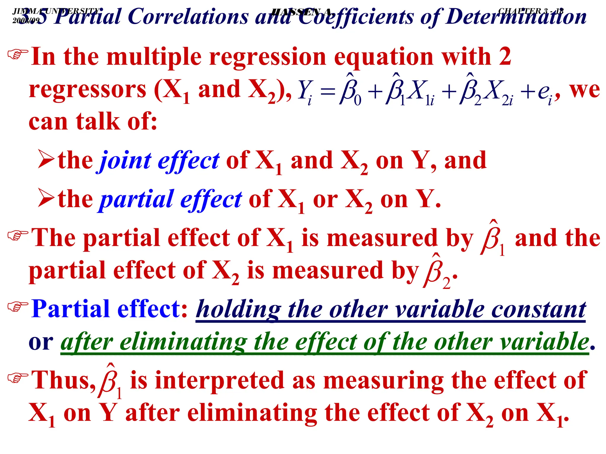
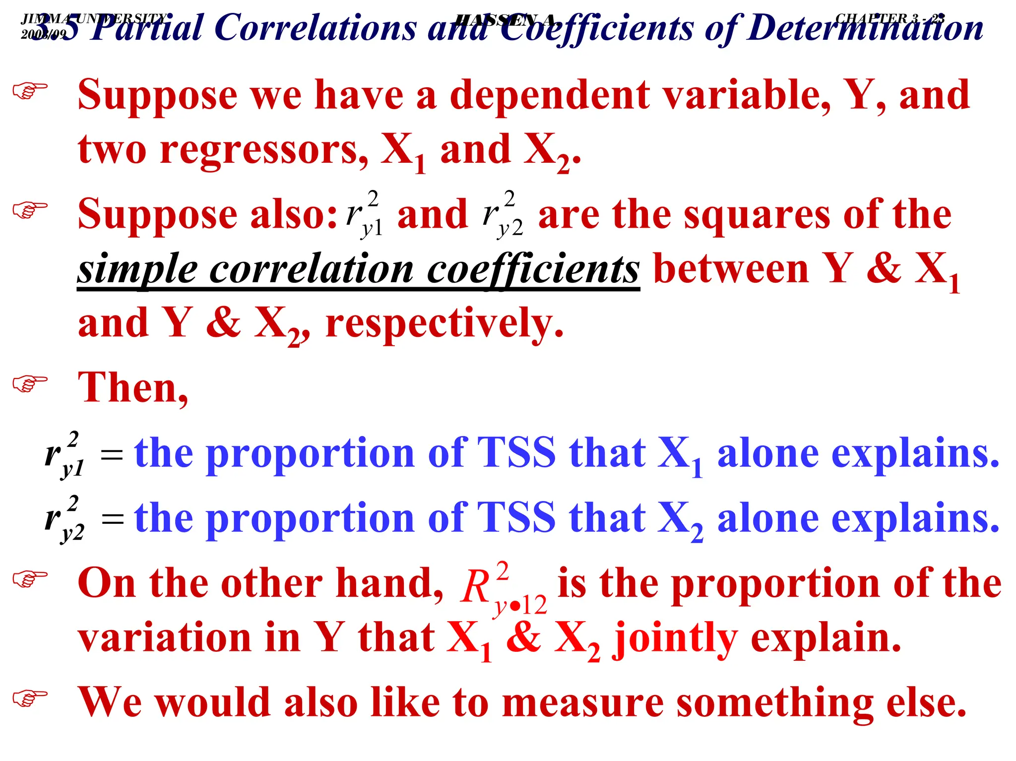
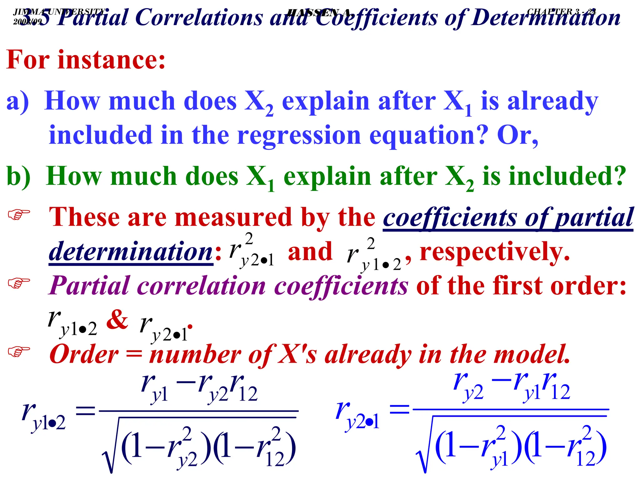
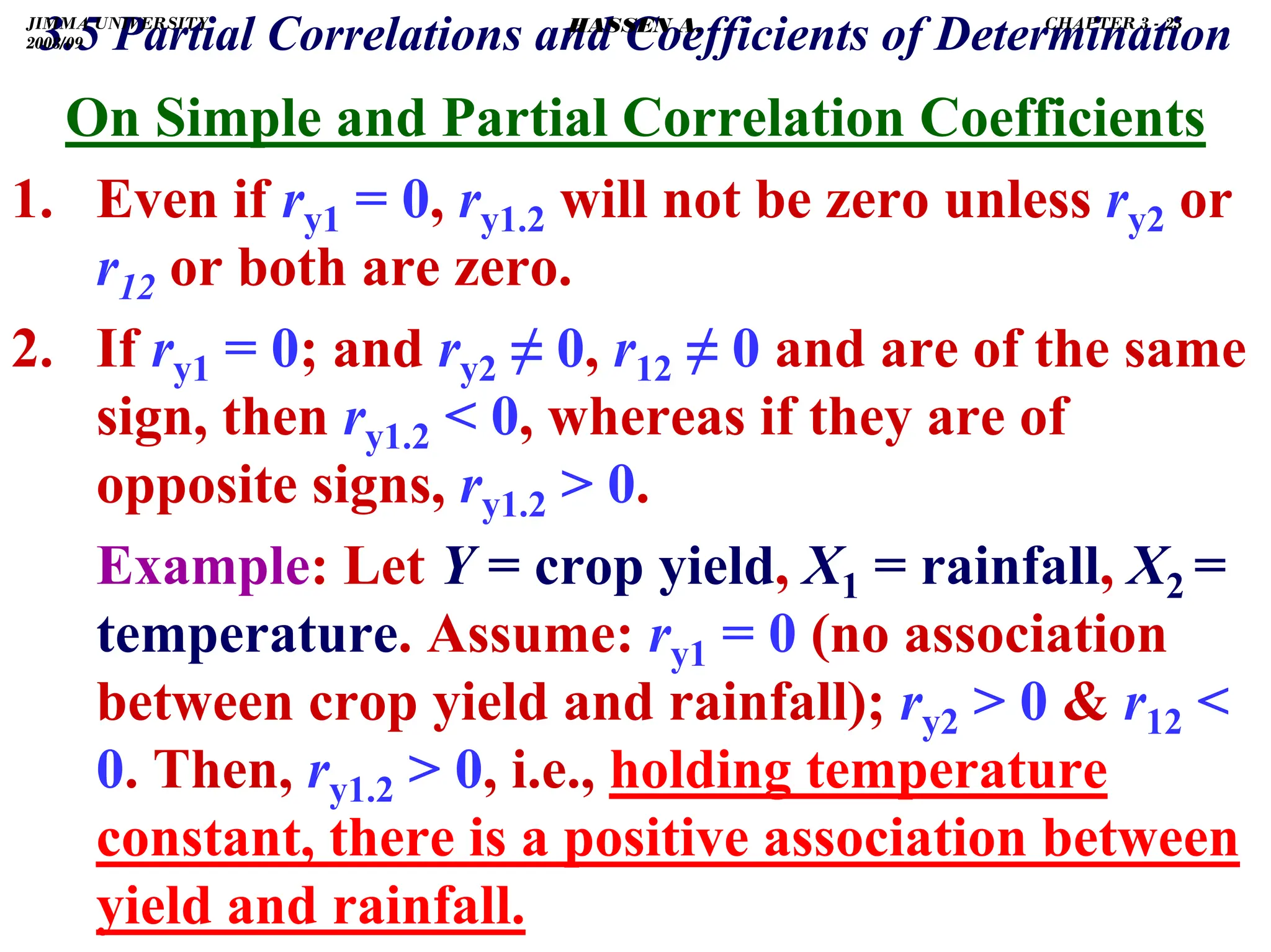
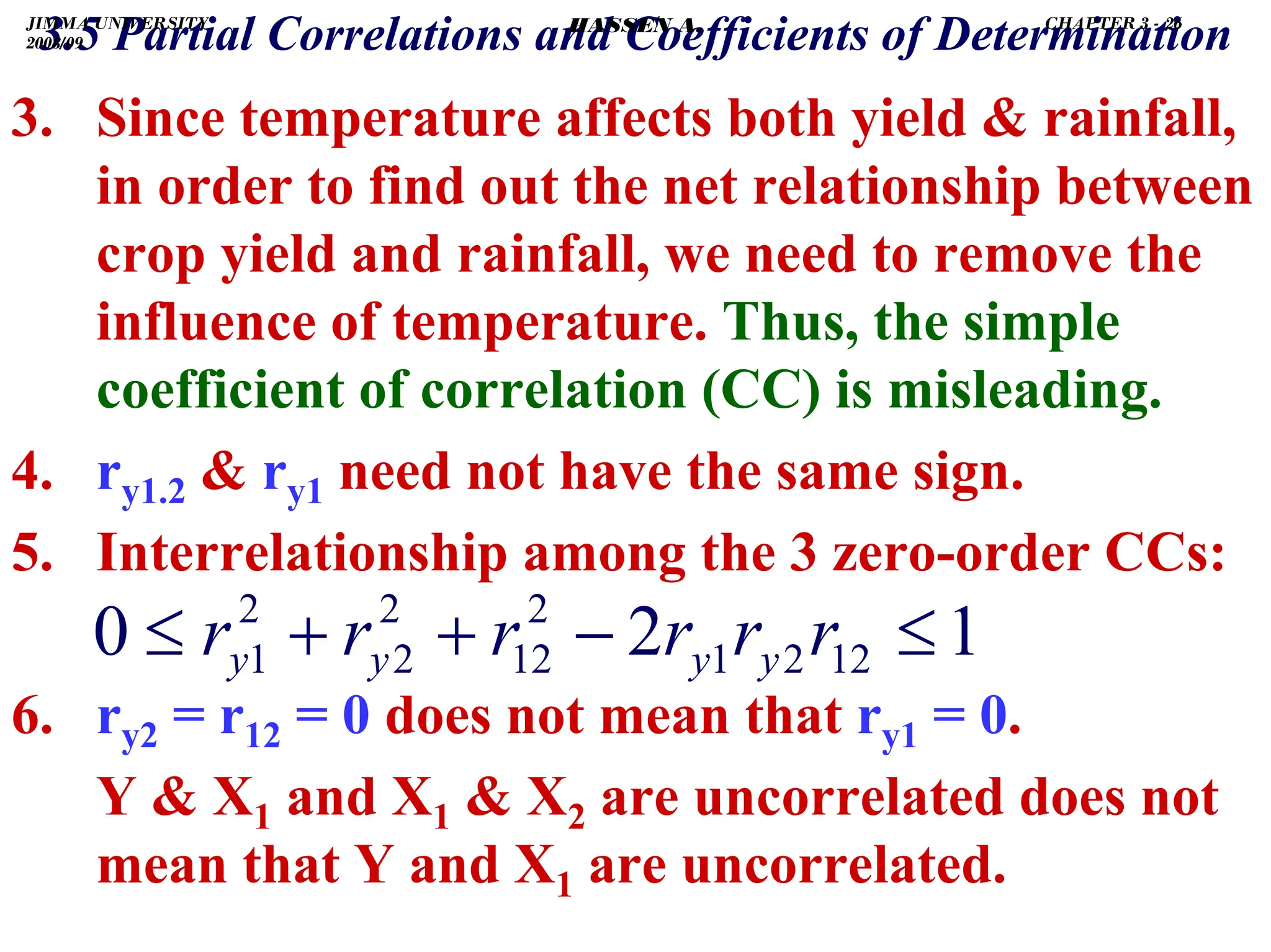
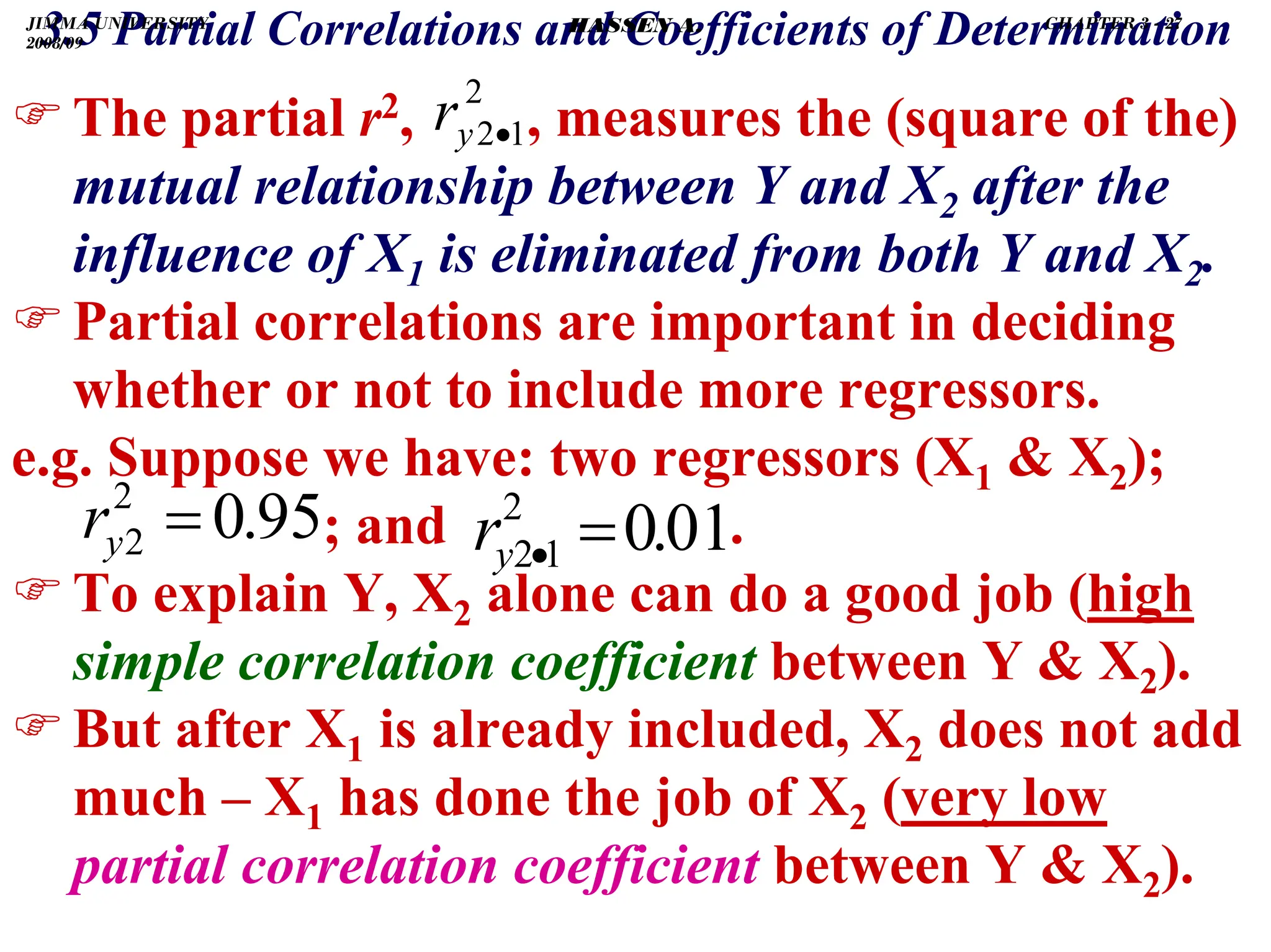
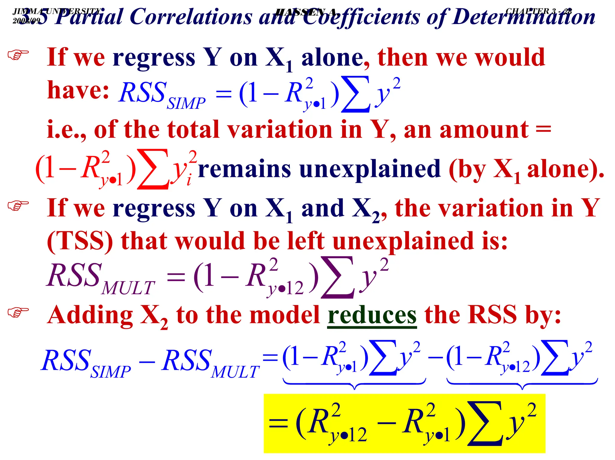
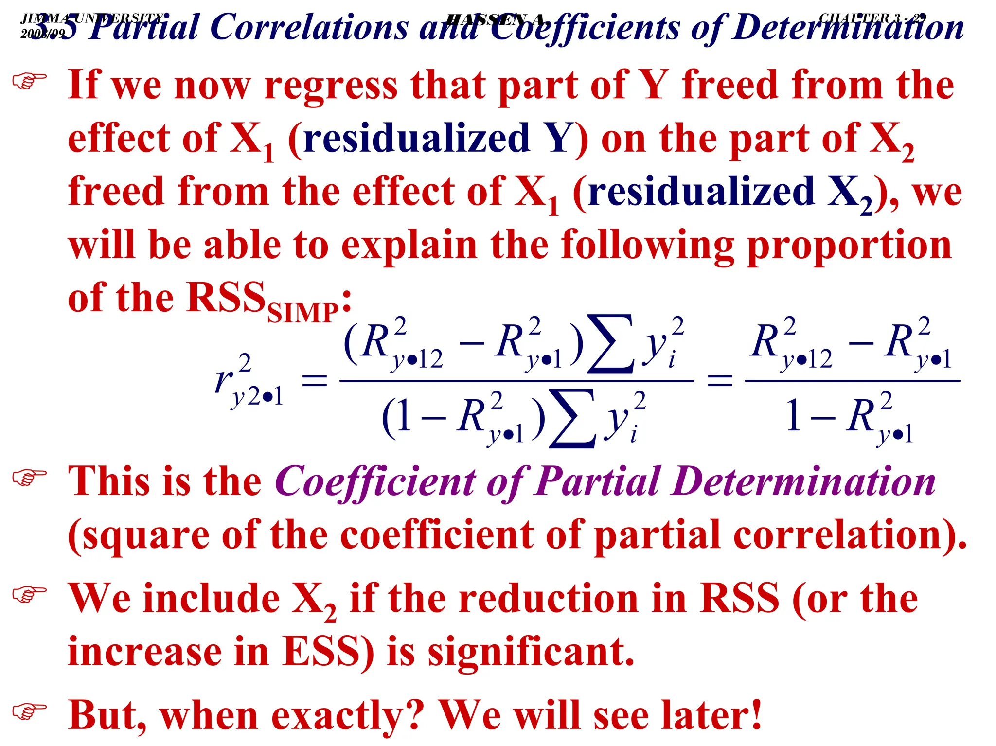
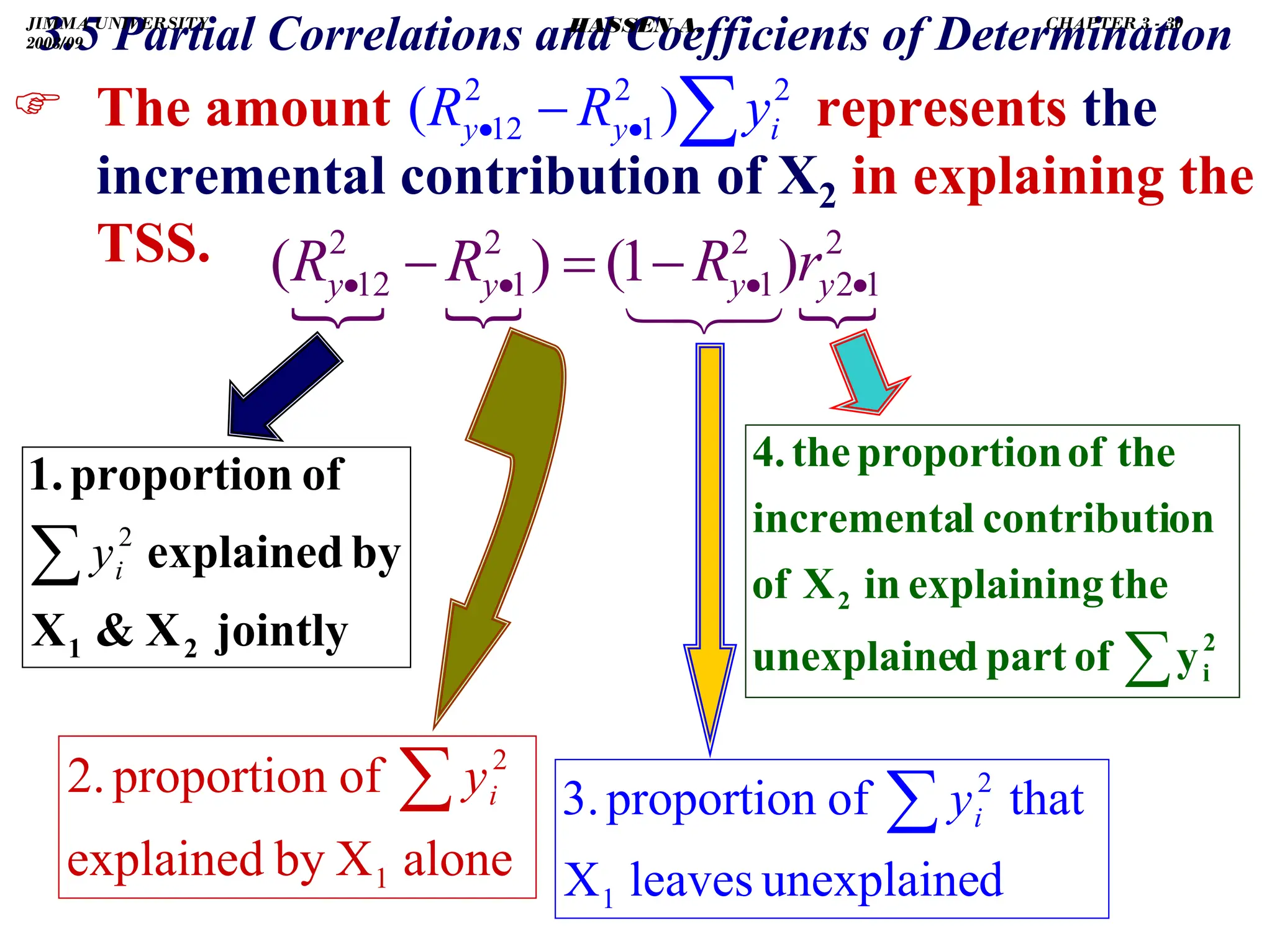
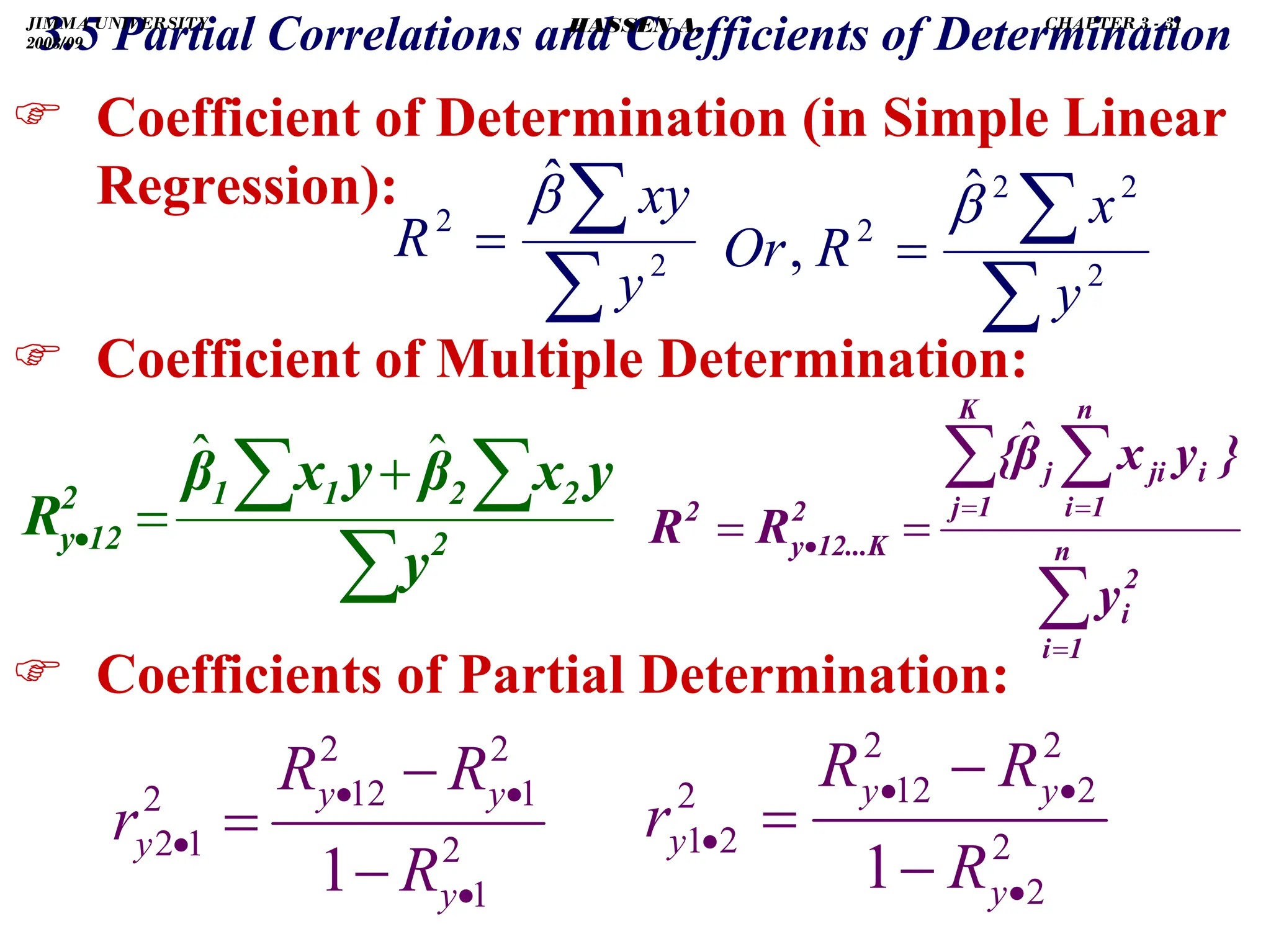
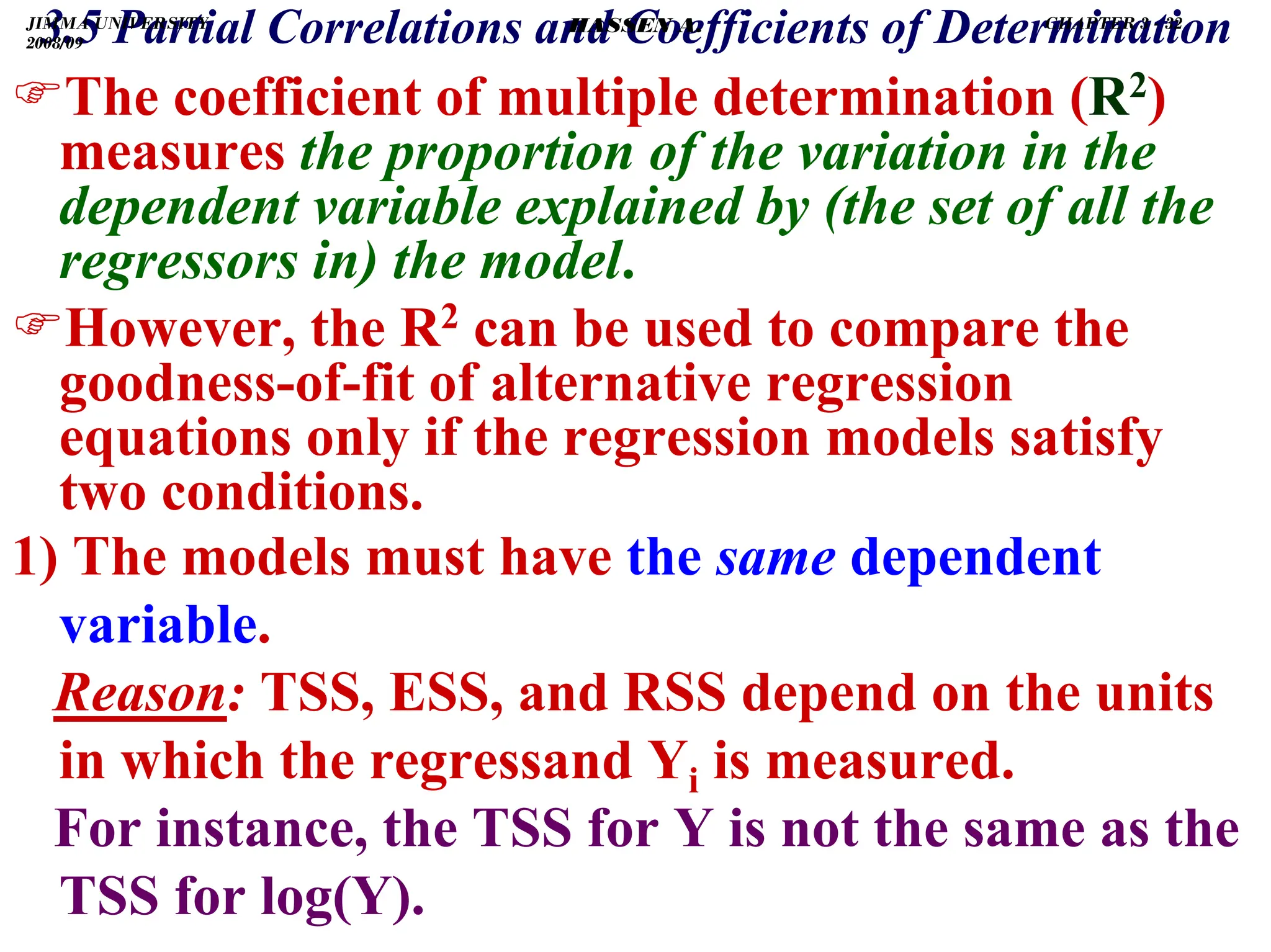
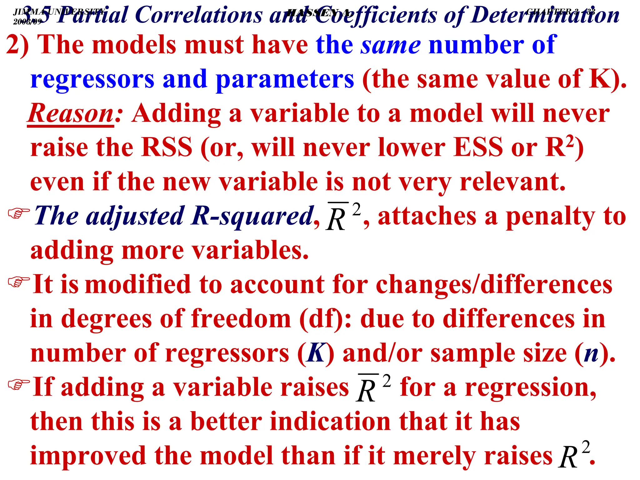
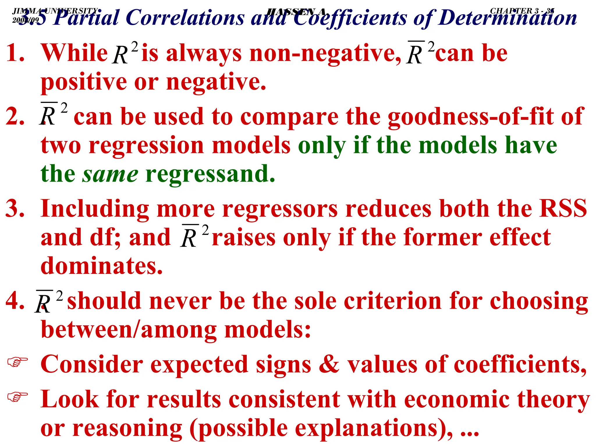
3.5 Partial Correlations and Coefficients of Determination
∑
∑
∑
∑
∑
∑
∑
∑
∑
∑
∑
−
+
−
=
⇒
2
1
2
2
2
1
2
2
2
2
2
2
1
2
1
2
2
2
2
1
1
)
(
2
)
(
)
(
x
x
x
x
x
x
x
x
x
x
yx
x
x
x
yx
bye
∑
∑
∑
∑
∑
∑
∑
∑
∑
∑
−
+
−
=
⇒
2
2
2
2
1
2
2
2
2
1
2
1
2
2
2
2
1
1
2
2
)
(
2
)
(
]
[
x
x
x
x
x
x
x
x
yx
x
x
yx
x
bye
∑
∑
∑
∑
∑
∑
∑
∑
∑
−
−
=
2
2
2
2
1
2
2
2
1
2
2
2
2
1
1
2
2
]
)
(
[
]
[
x
x
x
x
x
x
yx
x
x
yx
x
bye
2
2
1
2
2
2
1
2
2
1
1
2
2
)
(∑
∑
∑
∑
∑
∑
∑
−
−
=
x
x
x
x
yx
x
x
yx
x
bye
1
β̂
=
⇒ ye
b
JIMMA UNIVERSITY
2008/09
CHAPTER 3 - 21
HASSEN A.

117. .
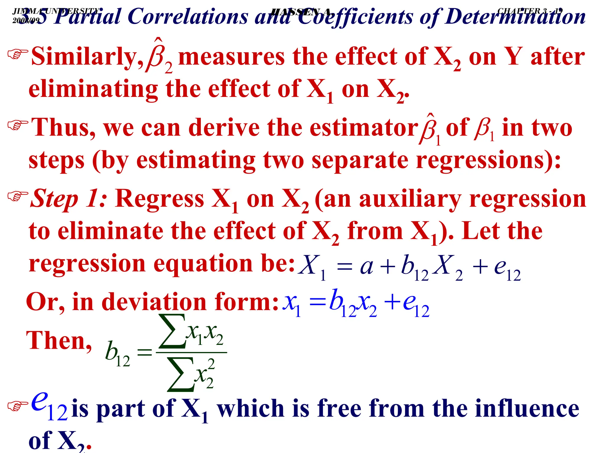
)Alternatively, we can derive the estimator of
as follows:
)Step 1: regress Y on X2, save the residuals, ey2.
…... [ey2 = residualized Y]
)Step 2: regress X1 on X2, save the residuals, e12.
…… [e12 = residualized X1]
)Step 3: regress ey2 (that part of Y cleared of the
influence of X2) on e12 (part of X1 cleared of the
influence of X2).
12
2
12
1
.
2 e
x
b
x
3.5 Partial Correlations and Coefficients of Determination
+
=
2
2
2
.
1 y
y e
x
b
y +
=
u
e
y +
= 12
12
2
e
.
3 α
!
ˆ
ˆ
ˆ
)
3
(
, 2
2
1
1 e
x
β
x
β
in y
sion
in regres
Then +
+
=
= 1
12 β
α
1
ˆ
β 1
β
JIMMA UNIVERSITY
2008/09
CHAPTER 3 - 22
HASSEN A.

118. .
) Suppose we have a dependent variable, Y, and
two regressors, X1 and X2.
) Suppose also: and are the squares of the
simple correlation coefficients between Y X1
and Y X2, respectively.
) Then,
the proportion of TSS that X1 alone explains.
the proportion of TSS that X2 alone explains.
) On the other hand, is the proportion of the
variation in Y that X1 X2 jointly explain.
) We would also like to measure something else.
2
1
y
r
2
12
•
y
R
2
2
y
r
=
2
y1
r
=
2
y2
r
3.5 Partial Correlations and Coefficients of Determination
JIMMA UNIVERSITY
2008/09
CHAPTER 3 - 23
HASSEN A.

119. .
For instance:
a) How much does X2 explain after X1 is already
included in the regression equation? Or,
b) How much does X1 explain after X2 is included?
) These are measured by the coefficients of partial
determination: and , respectively.
) Partial correlation coefficients of the first order:
.
) Order = number of X's already in the model.
2
2
1•
y
r
2
1
2•
y
r
2
1•
y
r 1
2•
y
r
3.5 Partial Correlations and Coefficients of Determination
)
1
)(
1
( 2
12
2
2
12
2
1
2
1
r
r
r
r
r
r
y
y
y
y
−
−
−
=
•
)
1
)(
1
( 2
12
2
1
12
1
2
1
2
r
r
r
r
r
r
y
y
y
y
−
−
−
=
•
JIMMA UNIVERSITY
2008/09
CHAPTER 3 - 24
HASSEN A.

120. .
On Simple and Partial Correlation Coefficients
1. Even if ry1 = 0, ry1.2 will not be zero unless ry2 or
r12 or both are zero.
2. If ry1 = 0; and ry2 ≠ 0, r12 ≠ 0 and are of the same
sign, then ry1.2 0, whereas if they are of
opposite signs, ry1.2 0.
Example: Let Y = crop yield, X1 = rainfall, X2 =
temperature. Assume: ry1 = 0 (no association
between crop yield and rainfall); ry2 0 r12
0. Then, ry1.2 0, i.e., holding temperature
constant, there is a positive association between
yield and rainfall.
3.5 Partial Correlations and Coefficients of Determination
JIMMA UNIVERSITY
2008/09
CHAPTER 3 - 25
HASSEN A.

121. .
3. Since temperature affects both yield rainfall,
in order to find out the net relationship between
crop yield and rainfall, we need to remove the
influence of temperature. Thus, the simple
coefficient of correlation (CC) is misleading.
4. ry1.2 ry1 need not have the same sign.
5. Interrelationship among the 3 zero-order CCs:
6. ry2 = r12 = 0 does not mean that ry1 = 0.
Y X1 and X1 X2 are uncorrelated does not
mean that Y and X1 are uncorrelated.
1
2
0 12
2
1
2
12
2
2
2
1 ≤
−
+
+
≤ r
r
r
r
r
r y
y
y
y
3.5 Partial Correlations and Coefficients of Determination
JIMMA UNIVERSITY
2008/09
CHAPTER 3 - 26
HASSEN A.

122. .
)The partial r2, , measures the (square of the)
mutual relationship between Y and X2 after the
influence of X1 is eliminated from both Y and X2.
)Partial correlations are important in deciding
whether or not to include more regressors.
e.g. Suppose we have: two regressors (X1 X2);
; and .
)To explain Y, X2 alone can do a good job (high
simple correlation coefficient between Y X2).
)But after X1 is already included, X2 does not add
much – X1 has done the job of X2 (very low
partial correlation coefficient between Y X2).
95
.
0
2
2 =
y
r 01
.
0
2
1
2 =
•
y
r
2
1
2•
y
r
3.5 Partial Correlations and Coefficients of Determination
JIMMA UNIVERSITY
2008/09
CHAPTER 3 - 27
HASSEN A.

123. .
) If we regress Y on X1 alone, then we would
have:
i.e., of the total variation in Y, an amount =
remains unexplained (by X1 alone).
) If we regress Y on X1 and X2, the variation in Y
(TSS) that would be left unexplained is:
) Adding X2 to the model reduces the RSS by:
∑
•
−
= 2
2
1 )
1
( y
R
RSS y
SIMP
∑
•
− 2
2
1)
1
( i
y y
R
∑
•
−
= 2
2
12 )
1
( y
R
RSS y
MULT
MULT
SIMP RSS
RSS −
3.5 Partial Correlations and Coefficients of Determination
∑
•
• −
= 2
2
1
2
12 )
( y
R
R y
y
∑
∑ •
• −
−
−
= 2
2
12
2
2
1 )
1
(
)
1
( y
R
y
R y
y
JIMMA UNIVERSITY
2008/09
CHAPTER 3 - 28
HASSEN A.

124. .
) If we now regress that part of Y freed from the
effect of X1 (residualized Y) on the part of X2
freed from the effect of X1 (residualized X2), we
will be able to explain the following proportion
of the RSSSIMP:
) This is the Coefficient of Partial Determination
(square of the coefficient of partial correlation).
) We include X2 if the reduction in RSS (or the
increase in ESS) is significant.
) But, when exactly? We will see later!
2
1
2
1
2
12
2
2
1
2
2
1
2
12
2
1
2
1
)
1
(
)
(
•
•
•
•
•
•
•
−
−
=
−
−
=
∑
∑
y
y
y
i
y
i
y
y
y
R
R
R
y
R
y
R
R
r
3.5 Partial Correlations and Coefficients of Determination
JIMMA UNIVERSITY
2008/09
CHAPTER 3 - 29
HASSEN A.

125. .
) The amount represents the
incremental contribution of X2 in explaining the
TSS.
alone
X
by
explained
of
proportion
2.
1
2
∑ i
y
2
1
2
2
1
2
1
2
12 )
1
(
)
( •
•
•
• −
=
− y
y
y
y r
R
R
R
∑
•
• − 2
2
1
2
12 )
( i
y
y y
R
R
jointly
X
X
by
explained
of
proportion
1.
2
1
∑ 2
i
y
d
unexplaine
leaves
X
that
of
proportion
3.
1
2
∑ i
y
∑ 2
i
2
y
of
part
d
unexplaine
the
explaining
in
X
of
on
contributi
l
incrementa
the
of
proportion
the
4.
3.5 Partial Correlations and Coefficients of Determination
JIMMA UNIVERSITY
2008/09
CHAPTER 3 - 30
HASSEN A.

126. .
) Coefficient of Determination (in Simple Linear
Regression):
) Coefficient of Multiple Determination:
) Coefficients of Partial Determination:
2
1
2
1
2
12
2
1
2
1 •
•
•
•
−
−
=
y
y
y
y
R
R
R
r
∑
∑
= 2
2
ˆ
y
xy
R
β
∑
∑ ∑
+
=
• 2
2
2
1
1
2
12
y
y
y
x
β
y
x
β
R
ˆ
ˆ
3.5 Partial Correlations and Coefficients of Determination
2
2
2
2
2
12
2
2
1
1 •
•
•
•
−
−
=
y
y
y
y
R
R
R
r
∑
∑ ∑
=
= =
• =
= n
1
i
2
i
K
1
j
n
1
i
i
ji
j
2
12...K
y
2
y
}
y
x
β
{
R
R
ˆ
∑
∑
= 2
2
2
2
ˆ
,
y
x
R
Or
β
JIMMA UNIVERSITY
2008/09
CHAPTER 3 - 31
HASSEN A.

127. .
3.5 Partial Correlations and Coefficients of Determination
)The coefficient of multiple determination (R2)
measures the proportion of the variation in the
dependent variable explained by (the set of all the
regressors in) the model.
)However, the R2 can be used to compare the
goodness-of-fit of alternative regression
equations only if the regression models satisfy
two conditions.
1) The models must have the same dependent
variable.
Reason: TSS, ESS, and RSS depend on the units
in which the regressand Yi is measured.
For instance, the TSS for Y is not the same as the
TSS for log(Y).
JIMMA UNIVERSITY
2008/09
CHAPTER 3 - 32
HASSEN A.

128. .
3.5 Partial Correlations and Coefficients of Determination
2) The models must have the same number of
regressors and parameters (the same value of K).
Reason: Adding a variable to a model will never
raise the RSS (or, will never lower ESS or R2)
even if the new variable is not very relevant.
)The adjusted R-squared, , attaches a penalty to
adding more variables.
)It is modified to account for changes/differences
in degrees of freedom (df): due to differences in
number of regressors (K) and/or sample size (n).
)If adding a variable raises for a regression,
then this is a better indication that it has
improved the model than if it merely raises .
2
R
2
R
2
R
JIMMA UNIVERSITY
2008/09
CHAPTER 3 - 33
HASSEN A.

129. .
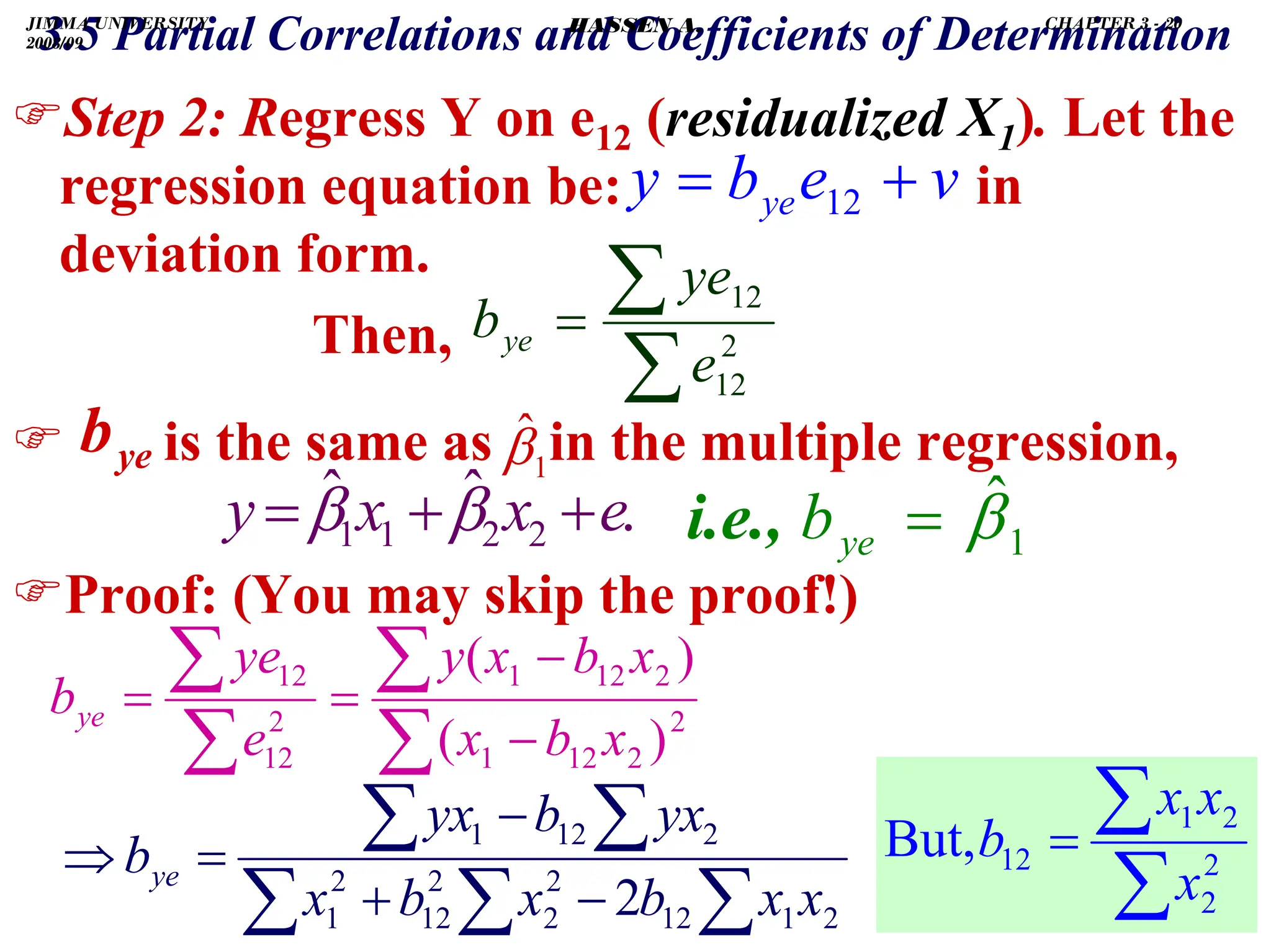
3.5 Partial Correlations and Coefficients of Determination
(Dividing TSS and RSS by their df).
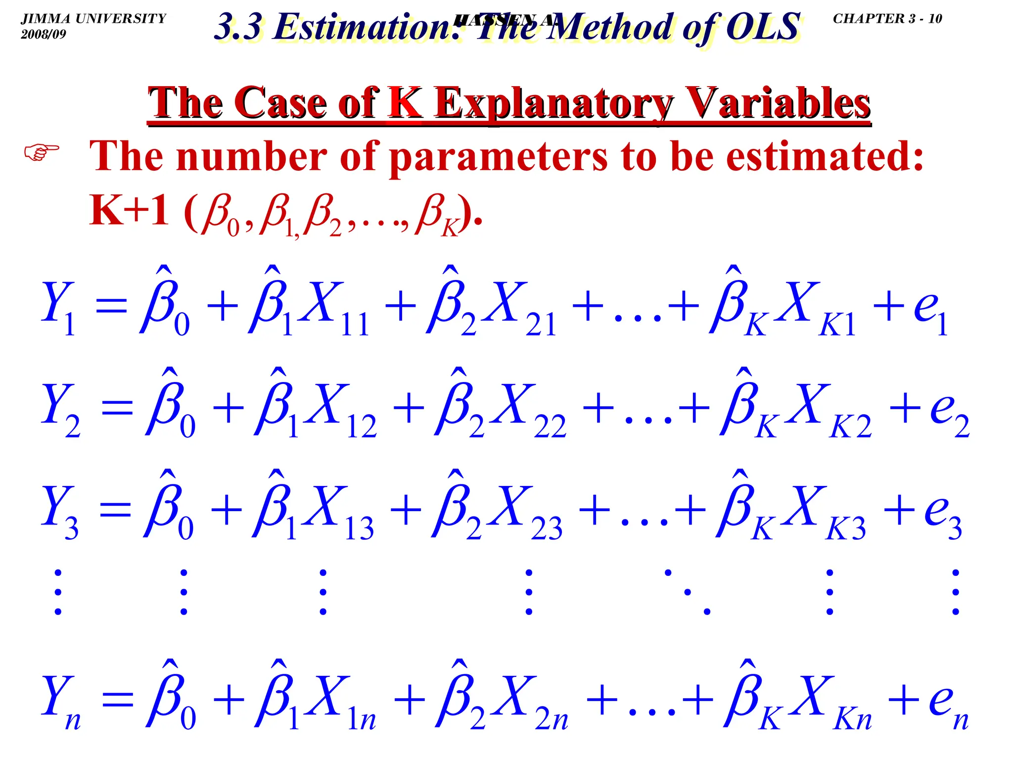
)K + 1 represents the number of parameters to be
estimated.
∑
∑
∑
∑ −
=
= 2
2
2
2
2
1
ˆ
y
e
y
y
R
]
[
]
[
1
n
y
1)
(K
n
e
1
R 2
2
2
−
+
−
−
=
∑
∑
]
1
1
[
1 2
2
2
−
−
−
•
−
=
∑
∑
K
n
n
y
e
R
)
1
1
(
)
1
(
1 2
2
−
−
−
•
−
−
=
K
n
n
R
R
)
1
1
(
)
1
(
1 2
2
−
−
−
•
−
=
−
K
n
n
R
R
2
2
2
2
2
2
1
1
,
1
R
R
R
R
R
R
K
≤
⇒
−
−
≥
general,
In
as
long
As
.
),
to
(relative
larger
grows
n
As
2
2
R
R
K →
JIMMA UNIVERSITY
2008/09
CHAPTER 3 - 34
HASSEN A.

130. .
3.5 Partial Correlations and Coefficients of Determination
1. While is always non-negative, can be
positive or negative.
2. . can be used to compare the goodness-of-fit of
two regression models only if the models have
the same regressand.
3. Including more regressors reduces both the RSS
and df; and raises only if the former effect
dominates.
4. . should never be the sole criterion for choosing
between/among models:
) Consider expected signs values of coefficients,
) Look for results consistent with economic theory
or reasoning (possible explanations), ...
2
R
2
R
2
R
2
R
2
R
JIMMA UNIVERSITY
2008/09
CHAPTER 3 - 35
HASSEN A.

131. .
Numerical Example:
Numerical Example:
Y (Salary in
'000 Dollars)
X1 (Years of post
high school
Education)
X2 (Years of
Experience)
30
30 4
4 10
10
20
20 3
3 8
8
36
36 6
6 11
11
24
24 4
4 9
9
40
40 8
8 12
12
ƩY = 150 ƩX1 = 25 ƩX2 = 50
JIMMA UNIVERSITY
2008/09
CHAPTER 3 - 36
HASSEN A.

132. .
Numerical Example:
Numerical Example:
X1Y X2Y X1
2 X2
2 X1X2
100
100 40
40
24
24
66
66
36
36
96
96
ƩX1X2
= 262
64
64
121
121
81
81
144
144
ƩX2
2
= 510
16
16
9
9
36
36
16
16
64
64
ƩX1
2
= 141
Y2
120
120 300
300 900
900
400
400
1296
1296
576
576
1600
1600
ƩY2 =
4772
60
60 160
160
216
216 396
396
96
96 216
216
320
320 480
480
n = 5
ƩX1 = 25
ƩX2 = 50
ƩY = 150
ƩYX1=812
ƩYX2=1567
ƩX1X2=262
ƩX1
2 = 141
ƩX2
2 = 510
ƩY2 = 4772
ƩX1Y
= 812
ƩX2Y
= 1552
JIMMA UNIVERSITY
2008/09
CHAPTER 3 - 37
HASSEN A.

133. .
Y
X
X
X '
' 1
)
(
ˆ −
=
β
⎟
⎟
⎟
⎠
⎞
⎜
⎜
⎜
⎝
⎛
•
⎥
⎥
⎥
⎦
⎤
⎢
⎢
⎢
⎣
⎡
=
⎟
⎟
⎟
⎟
⎠
⎞
⎜
⎜
⎜
⎜
⎝
⎛
∑
∑
∑
∑
∑
∑
∑
∑
∑
∑
∑
−
2
1
1
2
2
2
1
2
2
1
2
1
1
2
1
2
1
0
YX
YX
Y
X
X
X
X
X
X
X
X
X
X
n
β
β
β
ˆ
ˆ
ˆ
⎟
⎟
⎟
⎠
⎞
⎜
⎜
⎜
⎝
⎛
•
⎥
⎥
⎥
⎦
⎤
⎢
⎢
⎢
⎣
⎡
=
⎟
⎟
⎟
⎟
⎠
⎞
⎜
⎜
⎜
⎜
⎝
⎛ −
1552
812
150
510
262
50
262
141
25
50
25
5
β
β
β
1
2
1
0
ˆ
ˆ
ˆ
⎟
⎟
⎟
⎠
⎞
⎜
⎜
⎜
⎝
⎛
•
⎥
⎥
⎥
⎦
⎤
⎢
⎢
⎢
⎣
⎡
=
⎟
⎟
⎟
⎟
⎠
⎞
⎜
⎜
⎜
⎜
⎝
⎛
1552
812
150
1
0.75
-
6.25
-
0.75
-
0.625
4.375
6.25
-
4.375
40.825
β
β
β
2
1
0
ˆ
ˆ
ˆ
⎟
⎟
⎟
⎠
⎞
⎜
⎜
⎜
⎝
⎛
=
⎟
⎟
⎟
⎟
⎠
⎞
⎜
⎜
⎜
⎜
⎝
⎛
⇒
5.5
0.25
-
23.75
-
β
β
β
2
1
0
ˆ
ˆ
ˆ
2
1 X
5.5
X
0.25
23.75
Ŷ +
−
−
=
JIMMA UNIVERSITY
2008/09
CHAPTER 3 - 38
HASSEN A.

134. .
)One more year of experience, after controlling
for years of education, results in $5500 rise in
salary, on average.
)Or, if we consider two persons with the same
level of education, the one with one more year of
experience is expected to have a higher salary of
$5500.
)Similarly, for two people with the same level of
experience, the one with an education of one
more year is expected to have a lower annual
salary of $250.
)Experience looks far more important than
education (which has a negative sign).
JIMMA UNIVERSITY
2008/09
CHAPTER 3 - 39
HASSEN A.

135. .
) The constant term - 23.75 is the salary one
would get with no experience and no education.
) But, a negative salary is impossible.
) Then, what is wrong?
1. The sample must have been drawn from a
subgroup. We have persons with experience
ranging from 8 to 12 years (and post high
school education ranging from 3 to 8 years). So
we cannot extrapolate the results too far out of
this sample range.
2. Model specification: is our model correctly
specified (variables, functional form); does our
data set meet the underlying assumptions?
JIMMA UNIVERSITY
2008/09
CHAPTER 3 - 40
HASSEN A.

136. .
∑
∑ +
=
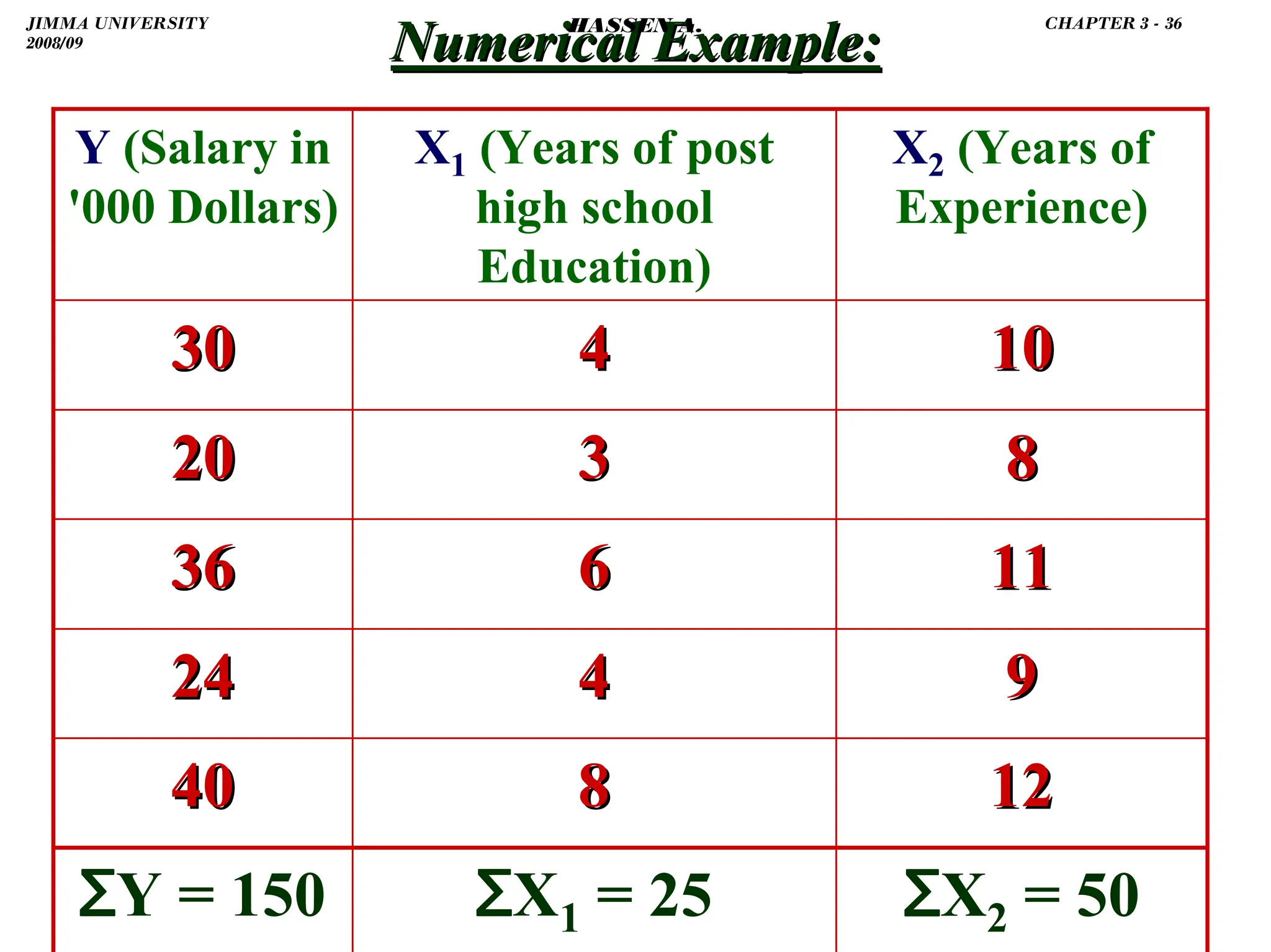
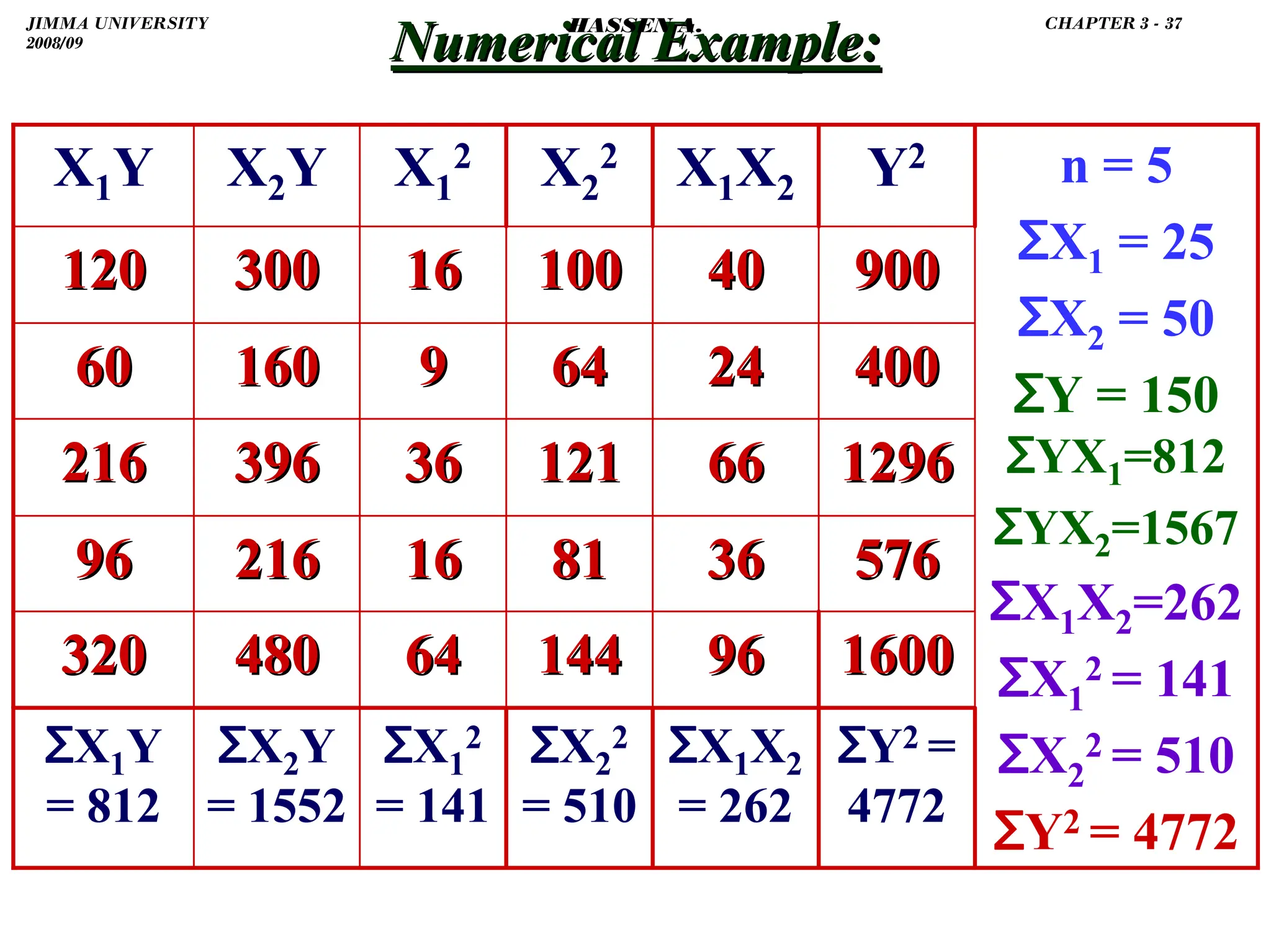
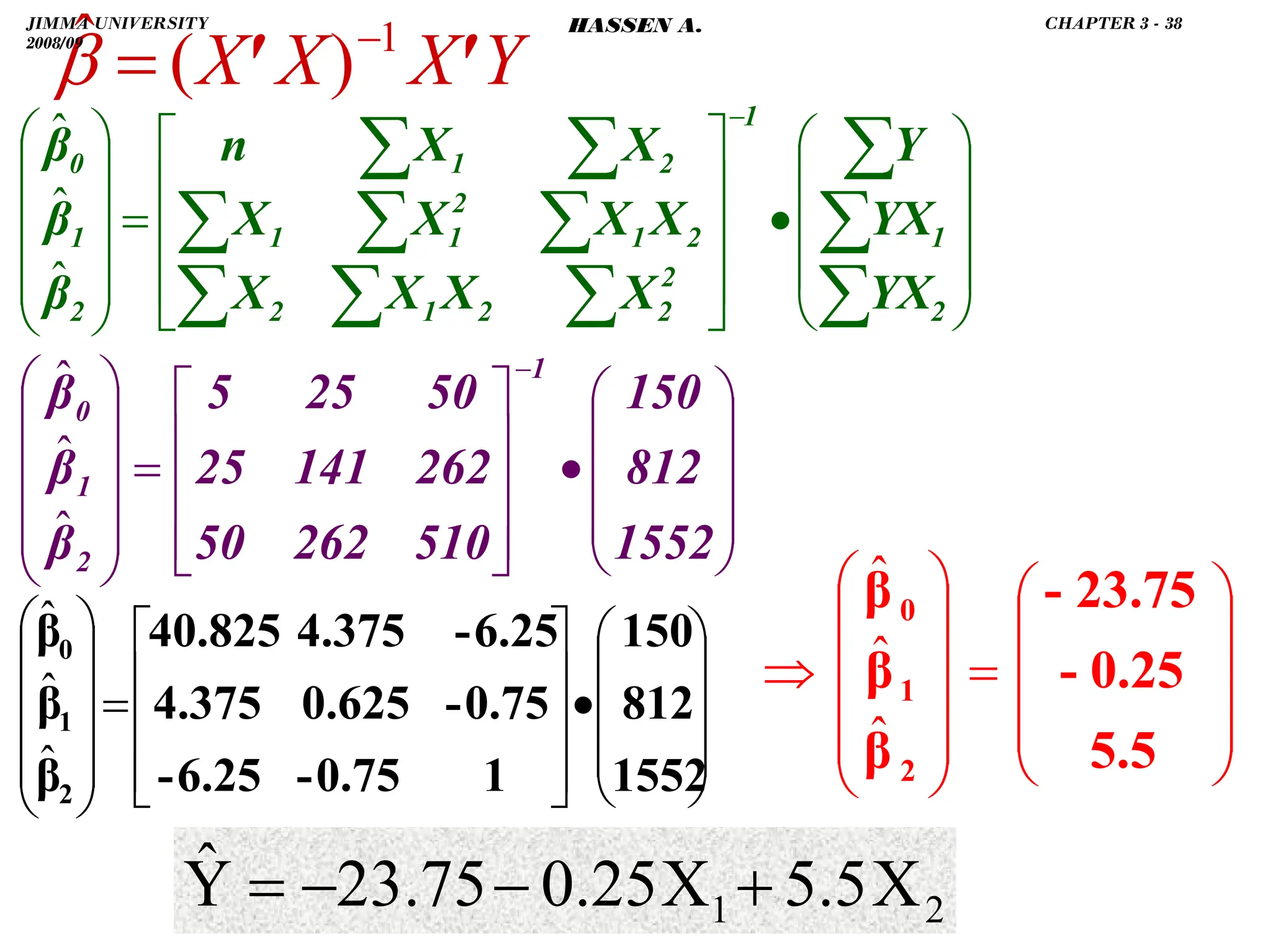
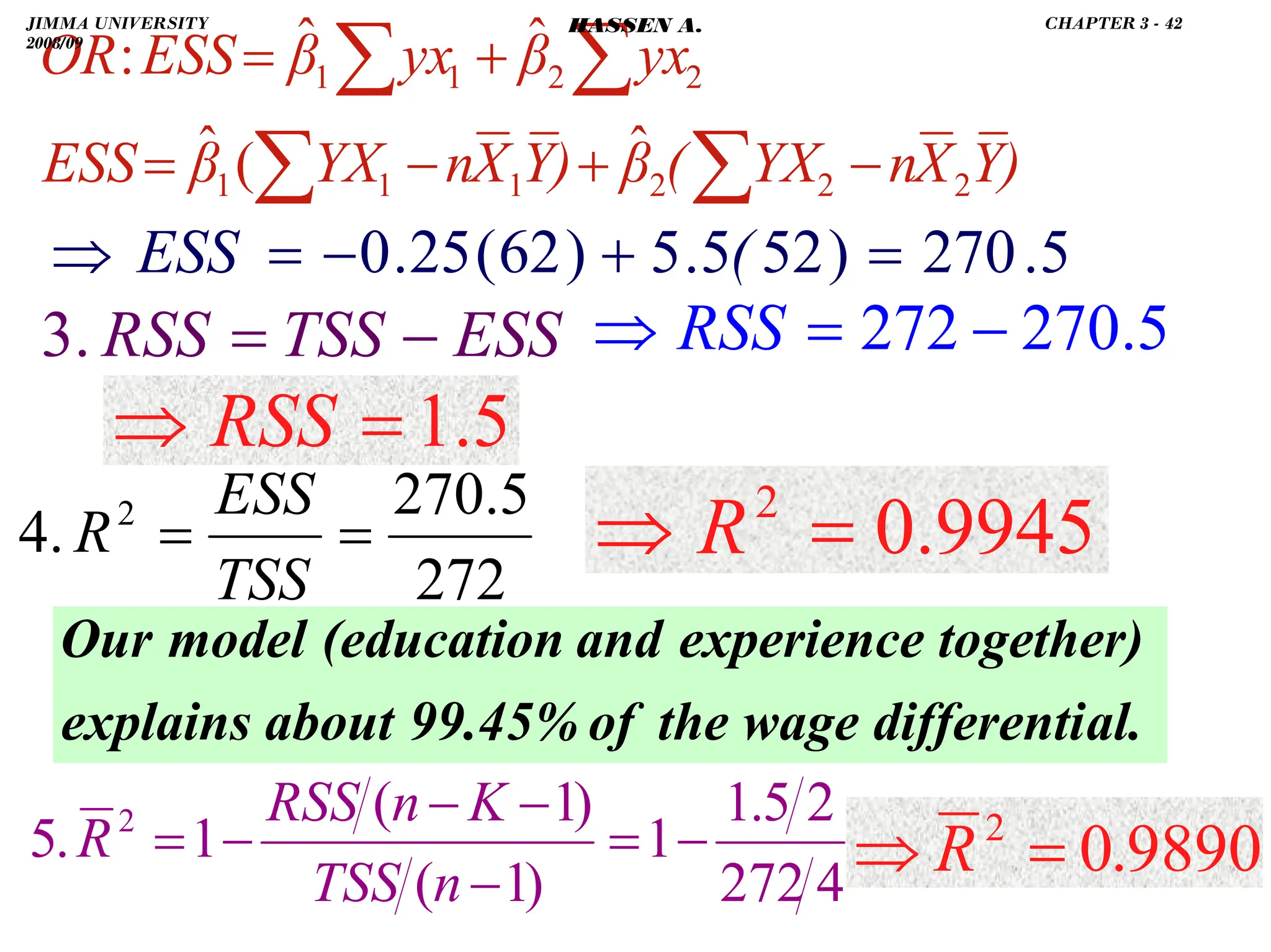
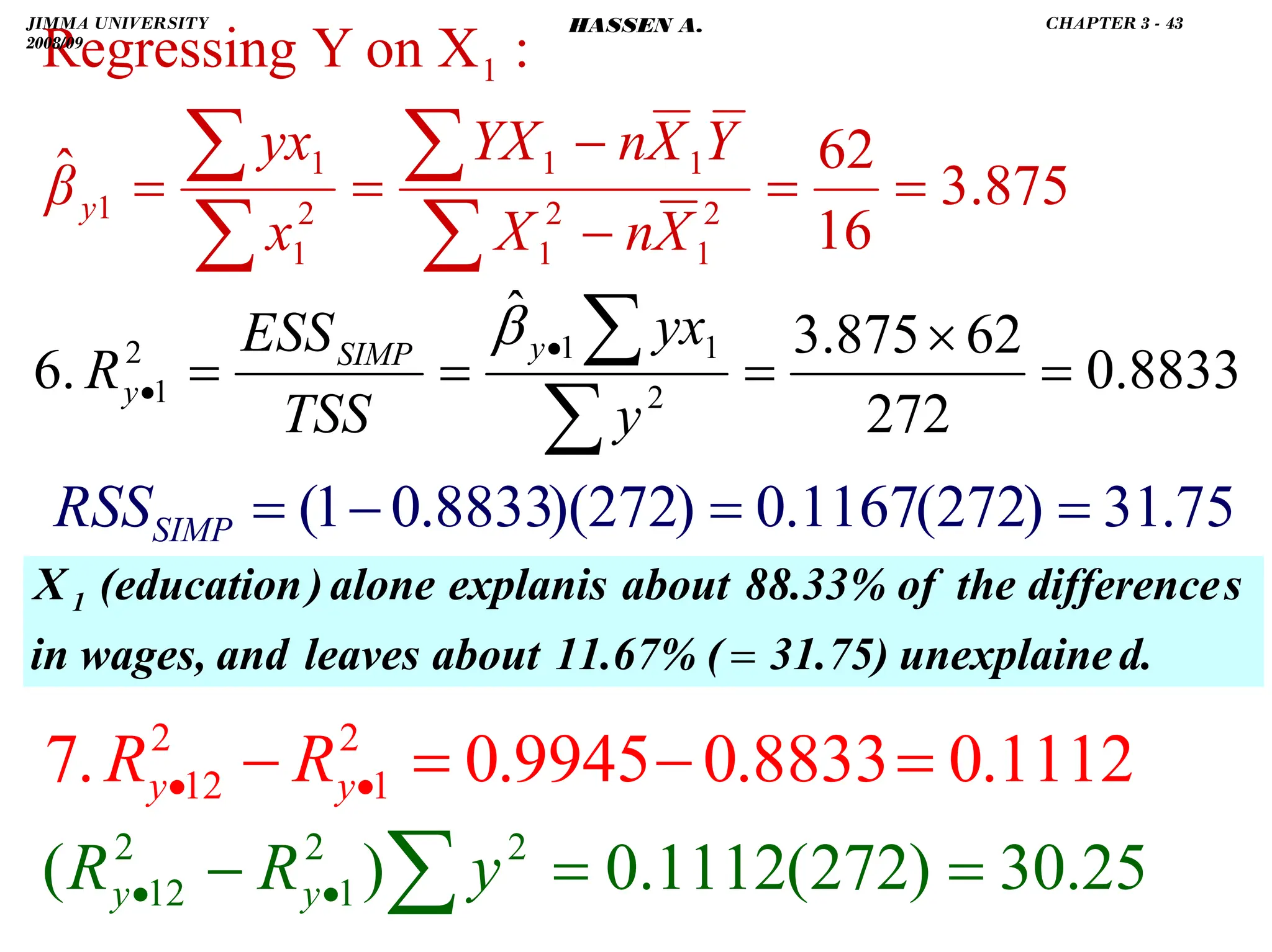
= 2
2
2
1
1
2 ˆ
ˆ
ˆ
.
2 )
x
β
x
β
(
y
ESS
2
2
2
.
1 Y
n
Y
y
TSS −
=
= ∑
∑
5(5)(10)]
[262
0.25)(5.5)
2(
]
5(10)
[510
(5.5)
]
5(5)
[141
0.25)
(
ESS 2
2
2
2
−
−
+
−
+
−
−
=
)
X
X
n
X
X
(
β
β
)
X
n
X
(
β
)
X
n
X
(
β
ESS
2
1
2
1
2
1
2
2
2
2
2
2
2
1
2
1
2
1
ˆ
ˆ
2
ˆ
ˆ
−
+
−
+
−
=
∑
∑
∑
270.5
ESS =
⇒
272
=
⇒ TSS
2
)
30
(
5
4772−
=
TSS
∑
∑
∑ +
+
= 2
1
2
1
2
2
2
2
2
1
2
1
ˆ
ˆ
2
ˆ
ˆ x
x
β
β
x
β
x
β
ESS
JIMMA UNIVERSITY
2008/09
CHAPTER 3 - 41
HASSEN A.

137. .
272
5
.
270
.
4 2
=
=
TSS
ESS
R
ESS
TSS
RSS −
=
.
3
)
Y
X
n
YX
(
β
)
Y
X
n
YX
β
ESS
yx
β
yx
β
ESS
OR
2
2
2
1
1
1
2
2
1
1
ˆ
(
ˆ
ˆ
ˆ
:
−
+
−
=
+
=
∑
∑
∑
∑
5
.
270
)
52
5
.
5
)
62
(
25
.
0 =
+
−
=
⇒ (
ESS
5
.
1
=
⇒ RSS
9945
.
0
2
=
⇒ R
al.
differenti
the wage
of
99.45%
about
explains
together)
experience
and
(education
model
Our
5
.
270
272 −
=
⇒ RSS
4
272
2
5
.
1
1
)
1
(
)
1
(
1
.
5 2
−
=
−
−
−
−
=
n
TSS
K
n
RSS
R 9890
.
0
2
=
⇒ R
JIMMA UNIVERSITY
2008/09
CHAPTER 3 - 42
HASSEN A.

138. . 8833
.
0
272
62
875
.
3
ˆ
.
6 2
1
1
2
1 =
×
=
=
=
∑
∑
•
•
y
yx
TSS
ESS
R
y
SIMP
y
β
875
.
3
16
62
ˆ
:
X
on
Y
Regressing
2
1
2
1
1
1
2
1
1
1
1
=
=
−
−
=
=
∑
∑
∑
∑
X
n
X
Y
X
n
YX
x
yx
βy
d.
unexplaine
31.75)
(
11.67%
about
leaves
and
wages,
in
s
difference
the
of
88.33%
about
explanis
alone
)
(education
X 1
=
75
.
31
)
272
(
1167
.
0
)
272
)(
8833
.
0
1
(
1112
.
0
8833
.
0
9945
.
0
.
7 2
1
2
12 =
−
=
− •
• y
y R
R
=
=
−
=
SIMP
RSS
25
.
30
)
272
(
1112
.
0
)
( 2
2
1
2
12 =
=
− ∑
•
• y
R
R y
y
JIMMA UNIVERSITY
2008/09
CHAPTER 3 - 43
HASSEN A.

139. .
wages.
in
variation
total
the
of
30.25)
(
11.12%
about
explaining
of
on
contributi
(marginal)
extra
an
with
equation
the wage
enters
e)
(experienc
X2
=
9528
.
0
8833
.
0
1
8833
.
0
9945
.
0
1
.
8 2
1
2
1
2
12
2
1
2 =
−
−
=
−
−
=
•
•
•
•
y
y
y
y
R
R
R
r
31.75).
(
d
unexplaine
left
has
X
that
al
differenti
the wage
of
30.25)
(
95.28%
about
explains
e)
(experienc
X
Or,
1
2
=
=
.
X
of)
influence
the
from
(free
to
related
not
is
which
X
of
part
the
of
on
contributi
the
is
this
that
Note
1
2
JIMMA UNIVERSITY
2008/09
CHAPTER 3 - 44
HASSEN A.

140. .
) The case of two regressors (X1 X2):
));
ˆ
var(
,
(
~
ˆ
0
0
0 β
β
β N
));
ˆ
var(
,
(
~
ˆ
1
1
1 β
β
β N
));
ˆ
var(
,
(
~
ˆ
2
2
2 β
β
β N
)
,
0
(
~ 2
σ
ε N
i
3.6 Statistical Inferences in Multiple Linear Regression
)
ˆ
,
ˆ
cov(
2
)
ˆ
var(
)
ˆ
var(
)
ˆ
var( 2
1
2
1
2
2
1
1
2
2
2
0 β
β
β
β
σ
β X
X
X
X
n
+
+
+
=
)
1
(
)
ˆ
var( 2
12
2
1
2
1
r
x i −
=
∑
σ
β
)
1
(
)
ˆ
var( 2
12
2
2
2
2
r
x i −
=
∑
σ
β
JIMMA UNIVERSITY
2008/09
CHAPTER 3 - 45
HASSEN A.

141. .
3.6 Statistical Inferences in Multiple Linear Regression
)
1
(
)
ˆ
,
ˆ
cov( 2
12
2
1
2
12
2
2
1
r
x
x
r
i
i −
−
=
∑
σ
β
β
∑
∑
∑
= 2
2
2
1
2
2
1
2
12
)
(
i
i
i
i
x
x
x
x
r
.
X
on
X
regressing
from
RSS
the
is
)
1
( 2
1
2
12
2
1 r
x i −
∑
.
X
on
X
regressing
from
RSS
the
is
)
1
( 1
2
2
12
2
2 r
x i −
∑
.
of
estimator
unbiased
an
is
3
ˆ 2
2
σ
n
RSS
−
=
σ
JIMMA UNIVERSITY
2008/09
CHAPTER 3 - 46
HASSEN A.

142. .
3.6 Statistical Inferences in Multiple Linear Regression
3.6 Statistical Inferences in Multiple Linear Regression
)Note that:
(a) (X'X)
(X'X)-
-1
1 is the same matrix we use to derive the
OLS estimates, and
(b) in the case of two regressors.
1
2
K
K
1
K
1
K
K
2
1
1
1
2
-1
/
2
X
X
X
X
X
X
X
X
X
X
n
σ
X)
(X
σ
β
−
⎥
⎥
⎥
⎥
⎥
⎦
⎤
⎢
⎢
⎢
⎢
⎢
⎣
⎡
=
=
−
∑
∑
∑
∑
∑
∑
∑
∑
…
…
…
)
ˆ
cov(
var
1
2
K
K
1
K
1
K
K
2
1
1
1
X
X
X
X
X
X
X
X
X
X
n
)
β
(
cοο
var
−
∧
⎥
⎥
⎥
⎥
⎥
⎦
⎤
⎢
⎢
⎢
⎢
⎢
⎣
⎡
=
−
∑
∑
∑
∑
∑
∑
∑
∑
…
…
…
2
ˆ
ˆ σ
3
ˆ
−
=
n
RSS
2
σ
JIMMA UNIVERSITY
2008/09
CHAPTER 3 - 47
HASSEN A.

143. .
) In the general case of K explanatory variables,
is an unbiased estimator of .
Note:
) Ceteris paribus, the higher the correlation
coefficient between X1 X2 ( ), the less
precise will the estimates be, i.e., the CIs
for the parameters will be wider.
) Ceteris paribus, the higher the degree of
variation of the Xjs (the more Xjs vary in our
sample), the more precise will the estimates be –
narrow CIs for population parameters.
2
1
ˆ
ˆ β
β
12
r
3.6 Statistical Inferences in Multiple Linear Regression
1
ˆ2
−
−
=
K
n
RSS
σ
2
σ
2
1 β
β
JIMMA UNIVERSITY
2008/09
CHAPTER 3 - 48
HASSEN A.

144. .
) The above two points are contained in:
where RSSj is the RSS from an auxiliary regres-
sion of Xj on all other (K–1) X's and a constant.
) We use t test to test about single parameters and
single linear functions of parameters.
) To test hypotheses about construct intervals
for individual use:
.
,...,
1
,
0
;
~
)
ˆ
(
ˆ
ˆ
1
*
K
j
t
e
s
K
n
j
j
j
=
∀
−
−
−
β
β
β
3.6 Statistical Inferences in Multiple Linear Regression
.
,...,
2
,
1
);
,
(
~
ˆ
2
K
j
RSS
N
j
j
j =
∀
σ
β
β
j
β
JIMMA UNIVERSITY
2008/09
CHAPTER 3 - 49
HASSEN A.

145. .
3.6 Statistical Inferences in Multiple Linear Regression
) Tests about and interval estimation of the error
variance are based on:
) Tests of several parameters and several linear
functions of parameters are F-tests.
Procedures for Conducting F-tests:
1. Compute the RSS from regressing Y on all Xjs
(URSS=Unrestricted Residual Sum of Squares).
2. Compute the RSS from the regression with the
hypothesized/specified values of parameters ( )
(RRSS = Restricted RSS).
2
1
K
n
2
2
2
χ
~
σ
σ̂
1)
K
(n
σ
RSS
−
−
−
−
=
2
σ
s
β
JIMMA UNIVERSITY
2008/09
CHAPTER 3 - 50
HASSEN A.

146. .
3.6 Statistical Inferences in Multiple Linear Regression
3. Under H0 (if the restriction is correct)
where J is the number of restrictions imposed.
If F-calculated is greater than the F-tabulated,
then the RRSS (is significantly) greater than the
URSS, and thus we reject the null.
) A special F-test of common interest is to test the
null that none of the Xs influence Y (i.e., that
our regression is useless!):
Test H0: vs. H1: H0 is not true.
0
...
2
1 =
=
=
= K
β
β
β
1
,
~
)
1
/(
/
)
(
−
−
−
−
−
K
n
J
F
K
n
URSS
J
URSS
RRSS
1
K
J,n
2
U
2
R
2
U
F
~
1)
K
)/(n
R
(1
)/J
R
(R
−
−
−
−
−
−
JIMMA UNIVERSITY
2008/09
CHAPTER 3 - 51
HASSEN A.

147. .
3.6 Statistical Inferences in Multiple Linear Regression
) With reference to our example on wages, test
the following at the 5% level of significance.
a) ; b) ; c) ;
d) the overall significance of the model; and
e) .
0
0 =
β
.
}
ˆ
{
)
1
(
1 1
2
2
2
∑ ∑
∑
∑ = =
−
=
−
=
K
j
n
i
i
ji
j
i
i y
x
y
y
R
URSS β
.
2
∑
= i
y
RRSS
1
,
2
2
~
)
1
/(
)
1
(
/
)
1
/(
/
)
(
−
−
−
−
−
=
−
−
−
⇒ K
n
K
F
K
n
R
K
R
K
n
URSS
K
URSS
RRSS
0
1 =
β 0
2 =
β
2
1 β
β =
JIMMA UNIVERSITY
2008/09
CHAPTER 3 - 52
HASSEN A.

148. .
1
2
)
(
)
ˆ
cov(
var −
=
− X
X'
σ
β
1
1
510
262
50
262
141
25
50
25
5
X)
(X'
−
−
⎥
⎥
⎥
⎦
⎤
⎢
⎢
⎢
⎣
⎡
=
⎥
⎥
⎥
⎦
⎤
⎢
⎢
⎢
⎣
⎡
=
1
0.75
-
6.25
-
0.75
-
0.625
4.375
6.25
-
4.375
40.825
1
ˆ
:
by
estimated
is 2
2
−
−
=
K
n
RSS
σ
σ 75
.
0
2
5
.
1
ˆ 2
=
=
σ
⎥
⎥
⎥
⎦
⎤
⎢
⎢
⎢
⎣
⎡
=
−
∧
1
0.75
-
6.25
-
0.75
-
0.625
4.375
6.25
-
4.375
40.825
0.75
)
β̂
(
cov
var
⎥
⎥
⎥
⎦
⎤
⎢
⎢
⎢
⎣
⎡
=
0.75
0.5625
-
4.6875
-
0.5625
-
0.4687
3.28125
4.6875
-
3.28125
30.61875
5
JIMMA UNIVERSITY
2008/09
CHAPTER 3 - 53
HASSEN A.

149. .
⎥
⎥
⎥
⎦
⎤
⎢
⎢
⎢
⎣
⎡
)
β
var(
)
β
,
β
cov(
)
β
var(
)
β
,
β
cov(
)
β
,
β
cov(
)
β
var(
2
2
1
1
2
0
1
0
0
ˆ
ˆ
ˆ
ˆ
ˆ
ˆ
ˆ
ˆ
ˆ
a)
b)
c) 29
.
4
61875
.
30
75
.
23
)
ˆ
(
ˆ
0
ˆ
0
0
−
≈
−
=
−
=
β
β
e
s
tc
30
.
4
2
025
.
0 ≈
=t
ttab
!
!
null!
the
reject
not
do
we
t
t tab
cal ⇒
≤ ,
37
.
0
46875
.
0
25
.
0
)
ˆ
(
ˆ
0
ˆ
1
1
−
≈
−
=
−
=
β
β
e
s
tc
null.
the
reject
not
do
we
,
t
t tab
cal ⇒
≤
35
.
6
75
.
0
5
.
5
)
ˆ
(
ˆ
0
ˆ
2
2
≈
=
−
=
β
β
e
s
tc
null.
the
reject
t
t tab
cal
⇒
⎥
⎥
⎥
⎦
⎤
⎢
⎢
⎢
⎣
⎡
=
0.75
0.5625
-
0.46876
4.6875
-
3.28125
30.61875
JIMMA UNIVERSITY
2008/09
CHAPTER 3 - 54
HASSEN A.

150. .
d)
e)
82
.
180
2
/
0055
.
0
2
/
9945
.
0
)
1
/(
)
1
(
/
2
2
≈
=
−
−
−
=
K
n
R
K
R
Fc
19
05
.
0
2
,
2 ≈
= F
Ft
null.
the
reject
,
F
F tab
cal ⇒
,
ˆ
ˆ
ˆ
ˆ
From 2
2
1
1
0 i
i
i X
X
Y β
β
β +
+
=
).
(
ˆ
ˆ
ˆ
ˆ
ˆ
ˆ
ˆ
run
Now
i
i
i
i
i
i
X
X
Y
X
X
Y
2
1
0
2
1
0
+
+
=
⇒
+
+
=
β
β
β
β
β
08
.
12
=
⇒ RRSS
5
.
1
=
URSS
51
.
18
05
.
0
2
,
1 ≈
= F
Ft
11
.
14
2
/
5
.
1
1
/
)
5
.
1
08
.
12
(
)
1
/(
)
(
/
)
(
≈
−
=
−
−
−
=
K
n
URSS
J
URSS
RRSS
Fc
null.
the
reject
not
do
we
,
F
F tab
cal ⇒
≤
JIMMA UNIVERSITY
2008/09
CHAPTER 3 - 55
HASSEN A.

151. .
3.6 Statistical Inferences in Multiple Linear Regression
) Note that we can also use t-test to test the single
restriction that β1 = β2 (equivalently, β1 - β2 = 0).
) The same result as the F-test, but the F-test is
easier to handle.
1
2
1
2
1
2
1
2
1
2
1
t
~
)
β̂
,
β̂
v(
ô
2c
)
β̂
r(
â
v
)
β̂
r(
â
v
β̂
β̂
)
β̂
β̂
(
ê
s
0
β̂
β̂
−
+
−
=
−
−
−
3.76
0.5625)
2(
0.8660254
0.6846532
5.75
tc −
≈
−
−
+
−
=
706
.
12
1
025
.
0 =
= t
tt
null.
the
reject
not
do
⇒
tab
cal t
t
JIMMA UNIVERSITY
2008/09
CHAPTER 3 - 56
HASSEN A.

152. .
3.6 Statistical Inferences in Multiple Linear Regression
To sum up
To sum up:
:
Assuming that our model is correctly specified
and all the assumptions are satisfied,
) Education (after controlling for experience)
doesn’t have a significant influence on wages.
) In contrast, experience (after controlling for
education) is a significant determinant of wages.
) The intercept parameter is also insignificant
(though at the margin). Less Important!
) Overall, the model explains a significant portion
of the observed wage pattern.
) We cannot reject the claim that the coefficients
of the two regressors are equal.
JIMMA UNIVERSITY
2008/09
CHAPTER 3 - 57
HASSEN A.

153. .
) In Chapter 2, we used the estimated simple
linear regression model for prediction: (i) mean
prediction (i.e., predicting the point on the
population regression function (PRF)), and (ii)
individual prediction (i.e., predicting an
individual value of Y), given the value of the
regressor X (say, X = X0).
) The formulas for prediction are also similar to
those in the case of simple regression except
that, to compute the standard error of the
predicted value, we need the variances and
covariances of all the regression coefficients.
3.7 Prediction with Multiple Linear Regression
JIMMA UNIVERSITY
2008/09
CHAPTER 3 - 58
HASSEN A.

154. .
Note:
) Even if the R2 for the SRF is very high, it does
not necessarily mean that our forecasts are
good.
) The accuracy of our prediction depends on the
stability of the coefficients between the period
used for estimation and the period used for
prediction.
) More care must be taken when the values of the
regressors (X's) themselves are forecasts.
3.7 Prediction with Multiple Linear Regression
JIMMA UNIVERSITY
2008/09
CHAPTER 3 - 59
HASSEN A.

155. .
CHAPTER FOUR
CHAPTER FOUR
VIOLATING THE ASSUMPTIONS OF
VIOLATING THE ASSUMPTIONS OF
THE CLASSICAL LINEAR
THE CLASSICAL LINEAR
REGRESSION MODEL (CLRM)
REGRESSION MODEL (CLRM)
JIMMA UNIVERSITY
2008/09
CHAPTER 4 - 1
HASSEN A.

156. .
) The estimates derived using OLS techniques
and the inferences based on those estimates are
valid only under certain conditions.
) In general, these conditions amount to the
regression model being well-specified.
) A regression model is statistically well-specified
for an estimator (say, OLS) if all of the
assumptions required for the optimality of the
estimator are satisfied.
) The model will be statistically misspecified if
one/more of the assumptions are not satisfied.
4.1 Introduction
4.1 Introduction
JIMMA UNIVERSITY
2008/09
CHAPTER 4 - 2
HASSEN A.

157. .
)Before we proceed to testing for violations of (or
relaxing) the assumptions of the CLRM
sequentially, let us recall: (i) the basic steps in a
scientific enquiry (ii) the assumptions made.
I. The Major Steps Followed in a Scientific Study
I. The Major Steps Followed in a Scientific Study:
1.Specifying a statistical model consistent with
theory (or a model representing the theoretical
relationship between a set of variables).
)This involves at least two choices to be made:
A.The choice of variables to be included into
the model, and
4.1 Introduction
4.1 Introduction
JIMMA UNIVERSITY
2008/09
CHAPTER 4 - 3
HASSEN A.

158. .
B.The choice of the functional form of the link
(linear in variables, linear in logarithms of
the variables, polynomial in regressors, etc.)
2.Selecting an estimator with certain desirable
properties (provided that the regression model
in question satisfies a given set of conditions).
3.Estimating the model. When can one estimate a
model? (sample size? perfect multicollinearity?)
4.Testing for the validity of assumptions made.
5.a) If there is no evidence of misspecification, go
on to conducting statistical inferences.
4.1 Introduction
4.1 Introduction
JIMMA UNIVERSITY
2008/09
CHAPTER 4 - 4
HASSEN A.

159. .
5.b) If the tests show evidence of misspecification
in one or more relevant forms, then there are
two possible courses of action implied:
)If the precise form of model misspecification
can be established, then it may be possible to
find an alternative estimator that is optimal
under the particular sort of misspecification.
)Regard statistical misspecification as an
indication of a defective model. Then, search
an alternative, well-specified regression
model, and start over (return to Step 1).
4.1 Introduction
4.1 Introduction
JIMMA UNIVERSITY
2008/09
CHAPTER 4 - 5
HASSEN A.

160. .
4.1 Introduction
4.1 Introduction
II. The Assumptions of the CLRM:
II. The Assumptions of the CLRM:
A1
A1: n K+1. Otherwise, estimation is not possible.
A2
A2: No perfect multicollinearity among the X's.
Implication: any X must have some variation.
A3
A3: ɛi|Xji ~ IID(0,σ2) or
A3.1: var(ɛi|Xj) = σ2 (0 σ2 ∞).
A3.2: cov(ɛi,ɛs|Xj) = 0, for all i ≠ s; s = 1, …, n.
A4
A4: ɛi's are normally distributed: ɛi|Xj ~ N(0,σ2).
A5
A5: E(ɛi|Xj) = E(ɛi) = 0; i = 1, …, n j = 1, …, K.
A5.1: E(ɛi) = 0 and X’s are non-stochastic, or
A5.2: E(ɛiXji) = 0 or E(ɛi|Xj) = E(ɛi) with stochastic X’s.
Implication: ɛ is independent of Xj thus cov(ɛ,Xj) = 0.
⎩
⎨
⎧
≠
=
=
t
s
for
0
t
s
for
σ
)
X
|
ε
E(ε
2
j
t
s
JIMMA UNIVERSITY
2008/09
CHAPTER 4 - 6
HASSEN A.

161. .
)Generally speaking, the several tests for the
violations of the assumptions of the CLRM are
tests of model misspecification.
)The values of the test statistics for testing
particular H0's tend to reject these H0's when
the model is misspecified in some way.
e.g., tests for heteroskedasticity or autocorrelation
are sensitive to omission of relevant variables.
)A significant test statistic may indicate hetero-
skedastic (or autocorrelated) errors, but it may
also reflect omission of relevant variables.
4.1 Introduction
4.1 Introduction
JIMMA UNIVERSITY
2008/09
CHAPTER 4 - 7
HASSEN A.

162. .
1. Small Samples (A1?)
2. Multicollinearity (A2?)
3. Non-Normal Errors (A4?)
4. Non-IID Errors (A3?):
A. Heteroskedasticity (A3.1?)
B. Autocorrelation (A3.2?)
5. Endogeneity (A5?):
A. Stochastic Regressors and Measurement Error
B. Model Specification Errors:
a. Omission of Relevant Variables
b. Wrong Functional Form
c. Inclusion of Irrelevant Variables (?XXX)
d. Stability of Parameters
C. Simultaneity (or Reverse Causality)
4.1 Introduction
4.1 Introduction
Outline:
JIMMA UNIVERSITY
2008/09
CHAPTER 4 - 8
HASSEN A.

163. .
)Requirement for estimation: n K+1.
)If the number of data points (n) is small, it may
be difficult to detect violations of assumptions.
)With small n, it is hard to detect heteroskedast-
icity or nonnormality of ɛi's even when present.
)Though none of the assumptions is violated, a
linear regression with small n may not have
sufficient power to reject βj = 0, even if βj ≠ 0.
)If [(K+1)/n] 0.4, it will often be difficult to fit
a reliable model.
) Rule of thumb: aim to have n ≥ 6X ideally n ≥ 10X.
4.2 Sample Size: Problems with Few Data Points
4.2 Sample Size: Problems with Few Data Points
JIMMA UNIVERSITY
2008/09
CHAPTER 4 - 9
HASSEN A.

164. .
) Many social research studies use a large
number of predictors.
) Problems arise when the various predictors are
highly and linearly related (highly collinear).
) Recall that, in a multiple regression, only the
independent variation in a regressor (an X) is
used in estimating the coefficient of that X.
) If two X's (X1 X2) are highly correlated with
each other, then the coefficients of X1 X2 will
be determined by the minority of cases where
they don’t vary together (or overlap).
4.3 Multicollinearity
4.3 Multicollinearity
JIMMA UNIVERSITY
2008/09
CHAPTER 4 - 10
HASSEN A.

165. .
) Perfect multicollinearity: occurs when one (or
more) of the regressors in a model (e.g., XK) is a
linear function of other/s (Xi, i = 1, 2, …, K-1).
) For instance, if X2 = 2X1, then there is a perfect
(an exact) multicollinearity between X1 X2.
) Suppose, PRF: Y=β0+β1X1+β2X2, X2=2X1.
) The OLS technique yields 3 normal equations:
4.3 Multicollinearity
4.3 Multicollinearity
∑
∑
∑
∑
∑
∑
∑
∑
∑
∑
∑
+
+
=
+
+
=
+
+
=
2
i
2
2
i
2
i
1
1
i
2
0
i
2
i
i
2
i
1
2
2
i
1
1
i
1
0
i
1
i
i
2
2
i
1
1
0
i
X
β̂
X
X
β̂
X
β̂
X
Y
X
X
β̂
X
β̂
X
β̂
X
Y
X
β̂
X
β̂
β̂
n
Y
JIMMA UNIVERSITY
2008/09
CHAPTER 4 - 11
HASSEN A.

166. .
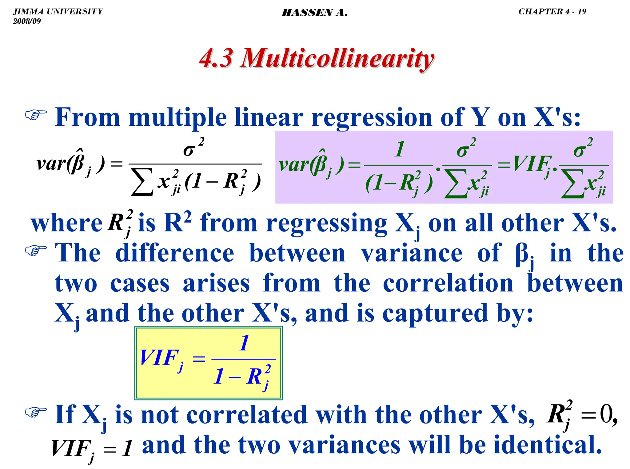
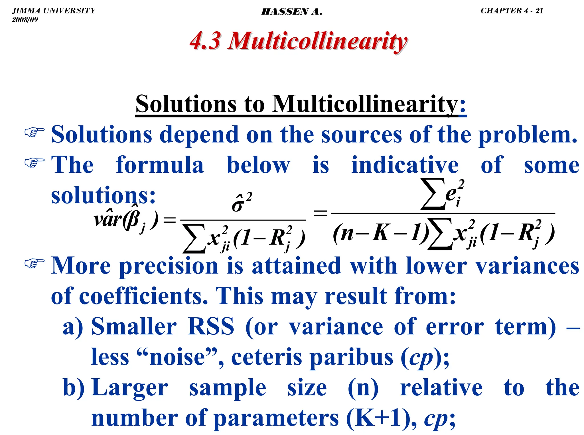
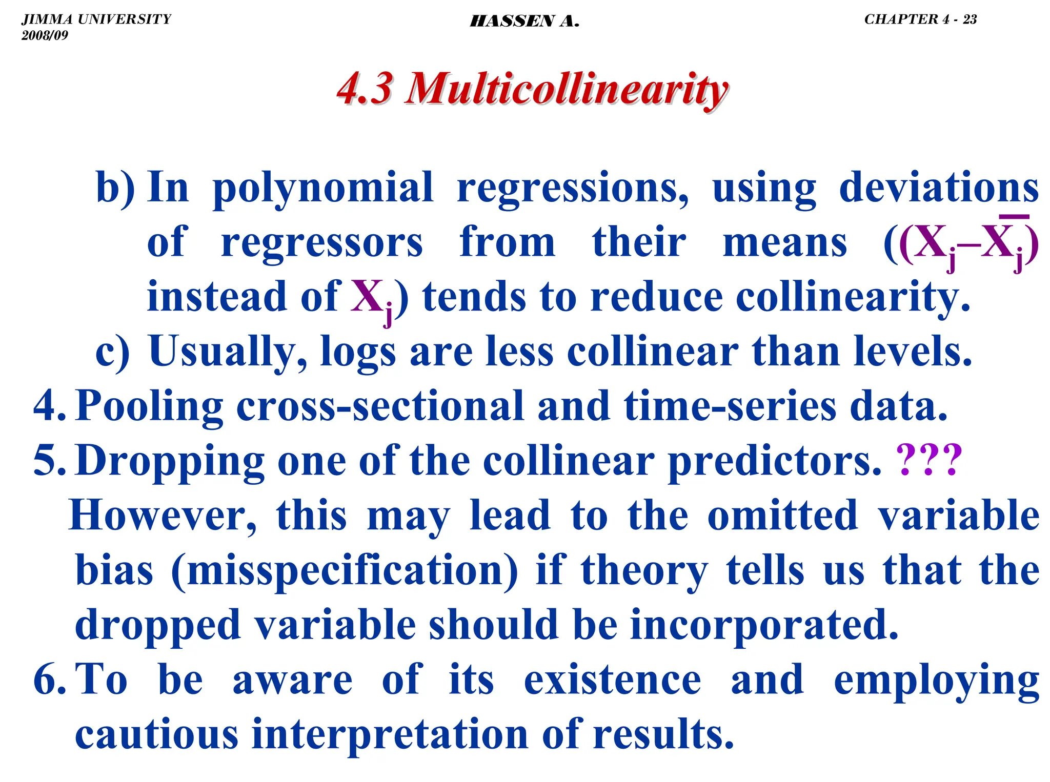
4.3 Multicollinearity
4.3 Multicollinearity
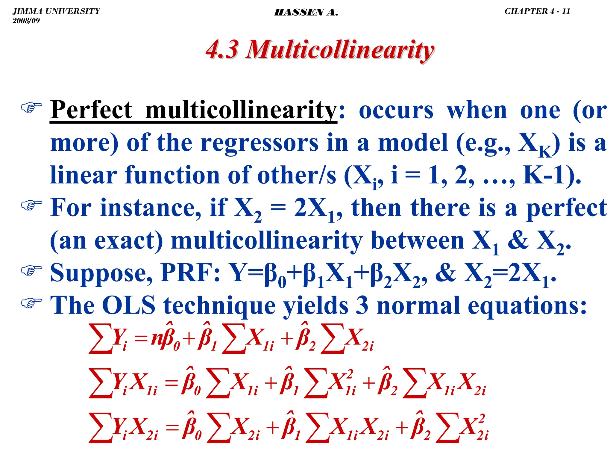
) But, substituting 2X1 for X2 in the 3rd equation
yields the 2nd equation.
) That is, one of the normal equations is in fact
redundant.
) Thus, we have only 2 independent equations (1
2 or 1 3) but 3 unknowns (β's) to estimate.
) As a result, the normal equations will reduce to:
∑
∑
∑
∑
∑
+
+
=
+
+
=
2
1
2
1
1
0
1
1
2
1
0
2
2
i
i
i
i
i
i
X
X
X
Y
X
n
Y
]
ˆ
ˆ
[
ˆ
]
ˆ
ˆ
[
ˆ
β
β
β
β
β
β
JIMMA UNIVERSITY
2008/09
CHAPTER 4 - 12
HASSEN A.

167. .
4.3 Multicollinearity
4.3 Multicollinearity
)The number of β's to be estimated is greater
than the number of independent equations.
)So, if two or more X's are perfectly correlated, it
is not possible to find the estimates for all β's.
i.e., we cannot find separately, but .
⎟
⎟
⎠
⎞
⎜
⎜
⎝
⎛
+
⎥
⎦
⎤
⎢
⎣
⎡
=
⎟
⎟
⎠
⎞
⎜
⎜
⎝
⎛
⇒
∑
∑
∑
∑
∑
2
1
0
2
1
1
1
1 2β
β
β
ˆ
ˆ
ˆ
.
i
i
i
i
i
i
X
X
X
n
X
Y
Y
2
1 β̂
β̂ 2
1 β̂
2
β̂ +
2
1
2
1i
1
1i
i
2
1
X
n
X
Y
X
n
X
Y
β̂
2
β̂
α̂
−
−
=
+
=
∑
∑
1
2
1
0 X
]
β̂
2
β̂
[
Y
β̂ +
−
=
JIMMA UNIVERSITY
2008/09
CHAPTER 4 - 13
HASSEN A.

168. .
)High, but not perfect, multicollinearity: two or
more regressors in a model are highly (but
imperfectly) correlated. e.g. X1 = 3 – 5XK + ui.
)This makes it difficult to isolate the effect of
each of the highly collinear X's on Y.
)If there is inexact but strong multicollinearity:
* The collinear regressors (X's) explain the
same variation in the regressand (Y).
* Estimated coefficients change dramatically,
depending on the inclusion/exclusion of
other predictor/s into (or out of) the model.
4.3 Multicollinearity
4.3 Multicollinearity
JIMMA UNIVERSITY
2008/09
CHAPTER 4 - 14
HASSEN A.

169. .
4.3 Multicollinearity
4.3 Multicollinearity
* . tend to be very shaky from one sample to
another.
* Standard errors of will be inflated.
* As a result, t-tests will be insignificant CIs
wide (rejecting H0: βj = 0 becomes very rare).
* We get low t-ratios but high R2 (or F): there
is not enough individual variation in the X's,
but a lot of common variation.
)Yet, the OLS estimators are BLUE
BLUE.
)BLUE – a property of repeated-sampling – says
nothing about estimates from a single sample.
s
'
β̂
s
'
β̂
JIMMA UNIVERSITY
2008/09
CHAPTER 4 - 15
HASSEN A.

170. .
4.3 Multicollinearity
4.3 Multicollinearity
) But, multicollinearity is not a problem if the
principal aim is prediction, given that the same
pattern of multicollinearity persists into the
forecast period.
Sources of Multicollinearity:
) Improper use of dummy variables. (Later!)
) Including the same (or almost the same)
variable twice (e.g. different operationaliaztions
of a single concept used together).
) Method of data collection used (e.g. sampling
over a limited range of X values).
JIMMA UNIVERSITY
2008/09
CHAPTER 4 - 16
HASSEN A.

171. .
4.3 Multicollinearity
4.3 Multicollinearity
)Including a variable computed from other
variables in the model (e.g. using family income,
mother’s income father’s income together).
)Adding many polynomial terms to a model,
especially if the range of the X variable is small.
)Or, it may just happen that variables are highly
correlated (without any fault of the researcher).
Detecting Multicollinearity:
)The classic case of multicollinearity occurs
when R2 is high ( significant), but none of X's
is significant (some of the X's may even have
wrong sign).
JIMMA UNIVERSITY
2008/09
CHAPTER 4 - 17
HASSEN A.

172. .
4.3 Multicollinearity
4.3 Multicollinearity
) Detecting the presence of multicollinearity is
more difficult in the less clear-cut cases.
) Sometimes, simple or partial coefficients of
correlation among regressors are used.
) However, serious multicollinearity may exist
even if these correlation coefficients are low.
) A statistic commonly used for detecting multi-
collinearity is VIF (Variance Inflation Factor).
) From a simple linear regression of Y on Xj we
have:
∑
= 2
ji
2
j
x
σ
)
β̂
var(
JIMMA UNIVERSITY
2008/09
CHAPTER 4 - 18
HASSEN A.

173. .
4.3 Multicollinearity
4.3 Multicollinearity
) From multiple linear regression of Y on X's:
where is R2 from regressing Xj on all other X's.
) The difference between variance of βj in the
two cases arises from the correlation between
Xj and the other X's, and is captured by:
) If Xj is not correlated with the other X's,
and the two variances will be identical.
)
R
(1
x
σ
)
β̂
var( 2
j
2
ji
2
j
−
=
∑
2
j
R
2
j
j
R
1
1
VIF
−
=
∑
∑
=
−
= 2
ji
2
j
2
ji
2
2
j
j
x
σ
.
VIF
x
σ
.
)
R
(1
1
)
β̂
var(
1
VIFj =
,
R2
j 0
=
JIMMA UNIVERSITY
2008/09
CHAPTER 4 - 19
HASSEN A.

174. .
4.3 Multicollinearity
4.3 Multicollinearity
) As Rj
2 increases, VIFj rises.
) If Xj is perfectly correlated with the other X's,
VIFj = ∞. Implication for precision (or CIs)???
) Thus, a large VIF is a sign of serious/severe (or
“intolerable”) multicollinearity.
) There is no cutoff point on VIF (or any other
measure) beyond which multicollinearity is
taken as intolerable.
) A rule of thumb: VIF 10
VIF 10 is a sign of severe
multicollinearity.
# In stata (after regression): vif
JIMMA UNIVERSITY
2008/09
CHAPTER 4 - 20
HASSEN A.

175. .
4.3 Multicollinearity
4.3 Multicollinearity
Solutions to Multicollinearity:
)Solutions depend on the sources of the problem.
)The formula below is indicative of some
solutions:
)More precision is attained with lower variances
of coefficients. This may result from:
a) Smaller RSS (or variance of error term) –
less “noise”, ceteris paribus (cp);
b) Larger sample size (n) relative to the
number of parameters (K+1), cp;
)
R
(1
x
1)
K
(n
e
2
j
2
ji
2
i
−
−
−
=
∑
∑
)
R
(1
x
σ̂
)
β̂
r(
â
v 2
j
2
ji
2
j
−
=
∑
JIMMA UNIVERSITY
2008/09
CHAPTER 4 - 21
HASSEN A.

176. .
4.3 Multicollinearity
4.3 Multicollinearity
c) Greater variation in values of each Xj, cp;
d) Less correlation between regressors, cp.
)Thus, serious multicollinearity may be solved by
using one/more of the following:
1.“Increasing sample size” (if possible). ???
2.Utilizing a priori information on parameters
(from theory or prior research).
3.Transforming variables or functional form:
a) Using differences (ΔX) instead of levels (X)
in time series data where the cause may be
X's moving in the same direction over time.
JIMMA UNIVERSITY
2008/09
CHAPTER 4 - 22
HASSEN A.

177. .
4.3 Multicollinearity
4.3 Multicollinearity
b) In polynomial regressions, using deviations
of regressors from their means ((Xj–X̅j)
instead of Xj) tends to reduce collinearity.
c) Usually, logs are less collinear than levels.
4.Pooling cross-sectional and time-series data.
5.Dropping one of the collinear predictors. ???
However, this may lead to the omitted variable
bias (misspecification) if theory tells us that the
dropped variable should be incorporated.
6.To be aware of its existence and employing
cautious interpretation of results.
JIMMA UNIVERSITY
2008/09
CHAPTER 4 - 23
HASSEN A.

178. .
4.4 Non
4.4 Non-
-normality of the Error Term
normality of the Error Term
)Normality is not required to get BLUE of β's.
)The CLRM merely requires errors to be IID.
)Normality of errors is required only for valid
hypothesis testing, i.e., validity of t- and F-tests.
)In small samples, if the errors are not normally
distributed, the estimated parameters will not
follow normal distribution, which complicates
inference.
)NB: there is no obligation on X's to be normally
distributed.
# In stata (after regression): kdensity residual, normal
JIMMA UNIVERSITY
2008/09
CHAPTER 4 - 24
HASSEN A.

179. .
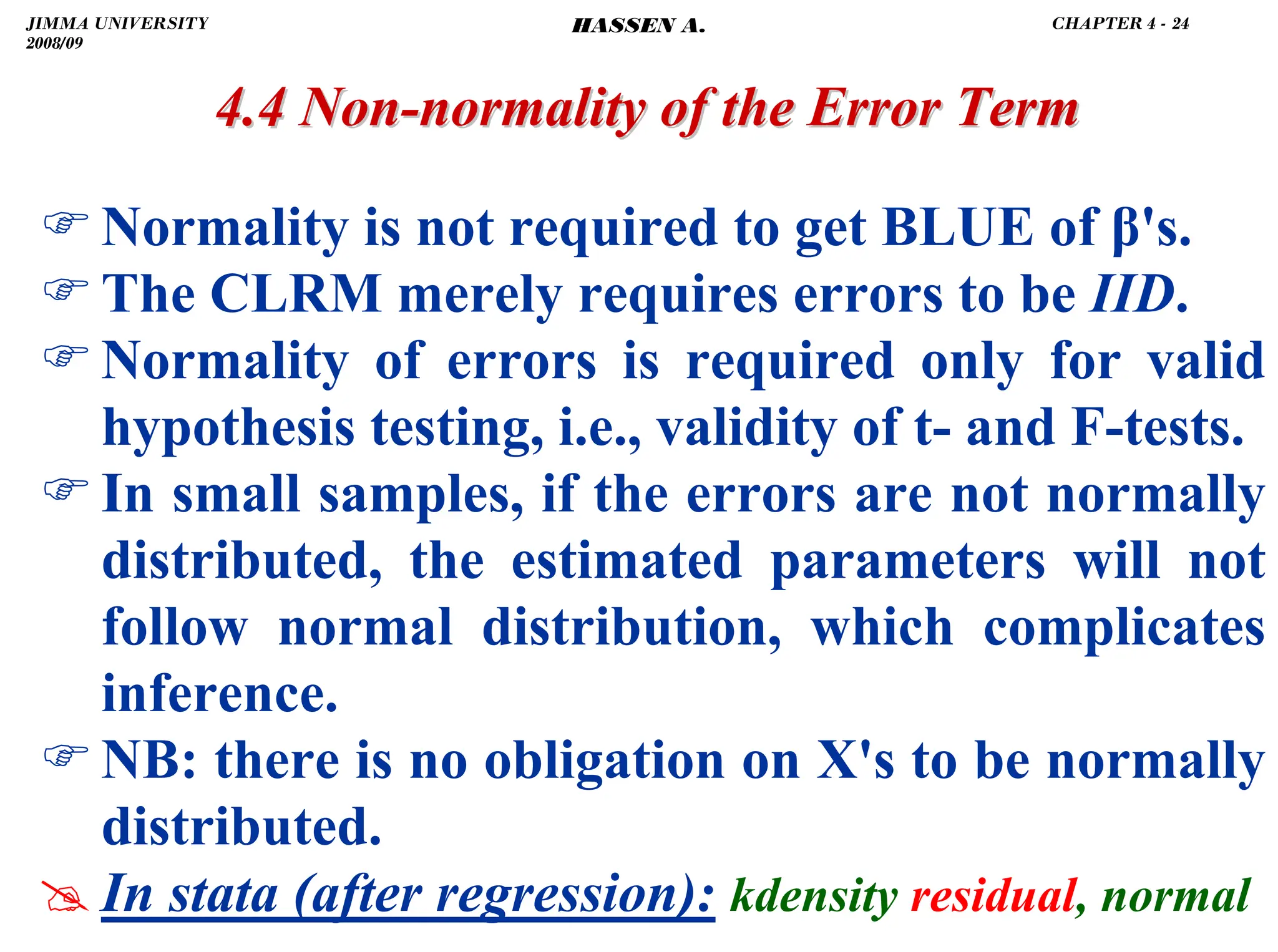
4.4 Non
4.4 Non-
-normality of the Error Term
normality of the Error Term
)A formal test of normality is the Shapiro-Wilk
test [H0: errors are normally distributed].
)Large p-value shows that H0 cannot be rejected.
#In stata: swilk residual
)If H0 is rejected, transforming the regressand or
re-specifying (the functional form of) the model
may help.
)With large samples, thanks to the central limit
theorem, hypothesis testing may proceed even if
distribution of errors deviates from normality.
)Tests are generally asymptotically valid.
JIMMA UNIVERSITY
2008/09
CHAPTER 4 - 25
HASSEN A.

180. .
)The assumption of IID errors is violated if a
(simple) random sampling cannot be assumed.
)More specifically, the assumption of IID errors
fails if the errors:
1) are not identically distributed, i.e., if var(εi|Xji)
varies with observations – heteroskedasticity.
2) are not independently distributed, i.e., if errors
are correlated to each other – serial correlation.
3) are both heteroskedastic autocorrelated.
This is common in panel time series data.
4.5 Non
4.5 Non-
-IID Errors
IID Errors
JIMMA UNIVERSITY
2008/09
CHAPTER 4 - 26
HASSEN A.

181. .
) One of the assumptions of the CLRM is homo-
skedasticity, i. e., var(εi|X) = var(εi) = σ2.
) This will be true if the observations of the error
term are drawn from identical distributions.
) Heteroskedasticity is present if var(εi)=σi
2≠σ2:
different variances for different segments of the
population (segments by the values of the X's).
e.g.: Variability of consumption rises with rise in
income, i.e., people with higher incomes display
greater variability in consumption.
) Heteroskedasticity is more likely in cross-
sectional than time-series data.
4.5.1
4.5.1 Heteroskedasticity
Heteroskedasticity
JIMMA UNIVERSITY
2008/09
CHAPTER 4 - 27
HASSEN A.

182. .
)With a correctly specified model (in any other
aspect), but heteroskedastic errors, the OLS
coefficient estimators are unbiased consistent
but inefficient.
)Reason: OLS estimator for σ2 (and thus for the
standard errors of the coefficients) are biased.
)Hence, confidence intervals based on biased
standard errors will be wrong, and the t F
tests will be misleading/invalid.
NB: Heteroskedasticity could be a symptom of
other problems (e.g. omitted variables).
4.5.1
4.5.1 Heteroskedasticity
Heteroskedasticity
JIMMA UNIVERSITY
2008/09
CHAPTER 4 - 28
HASSEN A.

183. .
) If heteroskedasticity is a result (or a reflection)
of specification error (say, omitted variables),
OLS estimators will be biased inconsistent.
) In the presence of heteroskedasticity, OLS is
not optimal as it gives equal weight to all
observations, when, in fact, observations with
larger error variances (σi
2) contain less
information than those with smaller σi
2 .
) To correct, give less weight to data points with
greater σi
2 and more weight to those with
smaller σi
2. [i.e., use GLS (WLS or FGLS)].
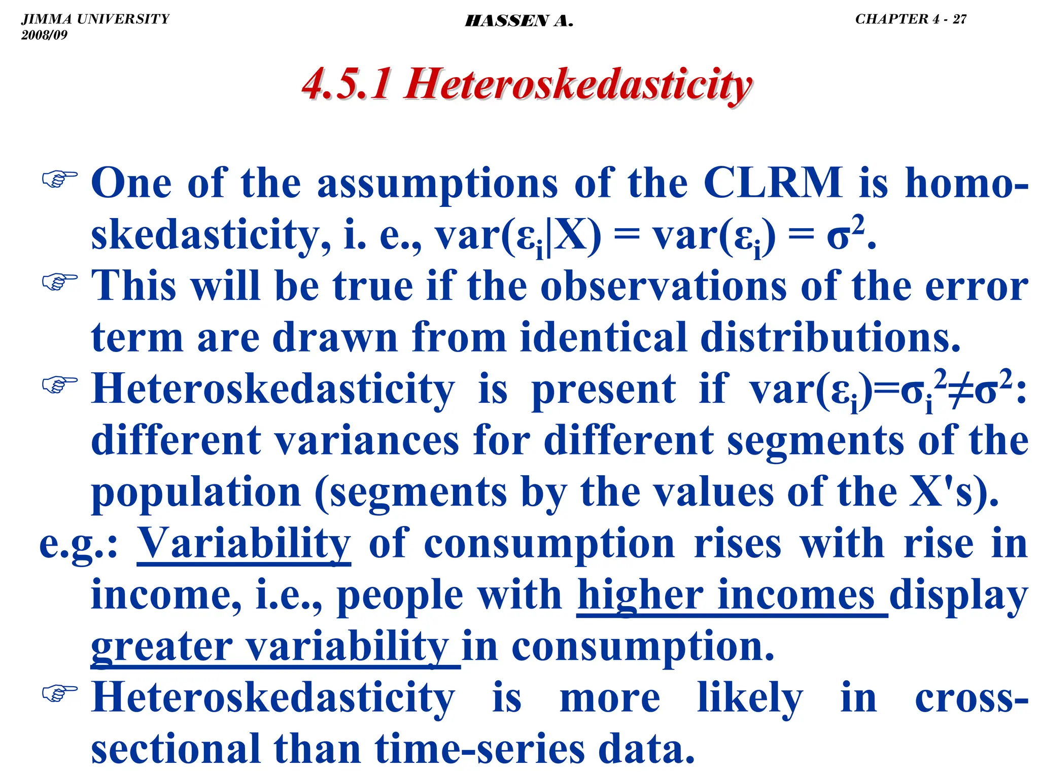
4.5.1
4.5.1 Heteroskedasticity
Heteroskedasticity
JIMMA UNIVERSITY
2008/09
CHAPTER 4 - 29
HASSEN A.

184. .
Detecting Heteroskedasticity:
Detecting Heteroskedasticity:
A. Graphical Method
) Run OLS and plot squared residuals versus
fitted value of Y (Ŷ) or against each X.
# In stata (after regression): rvfplot
) The graph may show some relationship (linear,
quadratic, …), which provides clues as to the
nature of the problem and a possible remedy.
e.g. let, the plot of ũ2 (from Y = α + βX + u) against
X signifies that var(ui) increases proportional
to X2; (var(ui)=σi
2 =cXi
2). What is the Solution?
4.5.1
4.5.1 Heteroskedasticity
Heteroskedasticity
JIMMA UNIVERSITY
2008/09
CHAPTER 4 - 30
HASSEN A.

185. .
4.5.1
4.5.1 Heteroskedasticity
Heteroskedasticity
) Now, transform the model by dividing Y, α, X
and u by X.
) Now, u* is homoskedastic: var(ui*) = c; i.e.,
using WLS solves heteroskedasticity!
) WLS yields BLUE for the transformed model.
) If the pattern of heteroskedasticity is unknown,
log transformation of both sides (compressing
the scale of measurement of variables) usually
solves heteroskedasticity.
) This cannot be used with 0 or negative values.
*
*
* u
x
y +
+
=
⇒ β
α
X
u
X
X
X
X
Y
+
+
= β
α
1
JIMMA UNIVERSITY
2008/09
CHAPTER 4 - 31
HASSEN A.

186. .
4.5.1
4.5.1 Heteroskedasticity
Heteroskedasticity
B. A Formal Test:
) The most-often used test for heteroskedasticity
is the Breusch-Pagan (BP) test.
H0: homoskedasticity vs. Ha: heteroskedasticity
) Regress ũ2 on Ŷ or ũ2 on the original X's, X2's
and, if enough data, cross-products of the X's.
) H0 will be rejected for high values of the test
statistic [n*R2~χ2
q] or for low p-values.
) n R2 are obtained from the auxiliary
regression of ũ2 on q (number of) predictors.
# In stata (after regression): hettest or hettest, rhs
JIMMA UNIVERSITY
2008/09
CHAPTER 4 - 32
HASSEN A.

187. .
4.5.1
4.5.1 Heteroskedasticity
Heteroskedasticity
)The B-P test as specified above:
9 uses the regression of ũ2 on Ŷ or on X's;
9 and thus consumes less degrees of freedom;
9 but tests for linear heteroskedasticity only;
9 and has problems when the errors are not
normally distributed.
# Alternatively, use: hettest, iid or hettest, rhs iid
This doesn’t need the assumption of normality.
)If you want to include squares cross products
of X's, generate these variables first and use:
# hettest varlist or hettest varlist, iid
)The hettest varlist, iid version of B-P test is the
same as White’s test for heteroskedasticity:
JIMMA UNIVERSITY
2008/09
CHAPTER 4 - 33
HASSEN A.

188. .
4.5.1
4.5.1 Heteroskedasticity
Heteroskedasticity
# In stata (after regression): imtest, white
Solutions to (or Estimation with) Heteroskedasticity
) If heteroskedasticity is detected, first check for
some other specification error in the model
(omitted variables, wrong functional form, …).
) If it persists even after correcting for other
specification errors, use one of the following:
1. Use better method of estimation (WLS/FGLS);
2. Stick to OLS but use robust (heteroskedasticity
consistent) standard errors.
# In stata: reg Y X1 … XK, robust
This is OK even with homoskedastic errors.
JIMMA UNIVERSITY
2008/09
CHAPTER 4 - 34
HASSEN A.

189. .
4.5.2 Autocorrelation
4.5.2 Autocorrelation
) Error terms are autocorrelated if error terms
from different (usually adjacent) time periods
(cross-sectional units) are correlated, E(εiεj)≠0.
) Autocorrelation in cross-sectional data is called
spatial autocorrelation (in space, not over time).
) However, spatial autocorrelation is uncommon
since cross-sectional data do not usually have
some ordering logic, or economic interest.
) Serial correlation occurs in time-series studies
when the errors associated with a given time
period carry over into future time periods.
JIMMA UNIVERSITY
2008/09
CHAPTER 4 - 35
HASSEN A.

190. .
4.5.2 Autocorrelation
4.5.2 Autocorrelation
) et are correlated with lagged values: et-1, et-2, …
) Effects of autocorrelation are similar to those
of heteroskedasticity:
) OLS coefficients are unbiased and consistent,
but inefficient; the estimate of σ2 is biased, and
thus inferences are invalid.
Detecting Autocorrelation
) Whenever you do on time series data, set up
your data as a time-series (i.e., identify the
variable that represents time or the sequential
order of observations).
# In stata: tsset varname
JIMMA UNIVERSITY
2008/09
CHAPTER 4 - 36
HASSEN A.

191. .
4.5.2 Autocorrelation
4.5.2 Autocorrelation
)Then, plotting OLS residuals against the time
variable, or a formal test could be used to check
for autocorrelation.
# In stata (after regression and predicting residuals):
scatter residual time
The Breusch-Godfrey Test
)Commonly-used general test of autocorrelation.
)It tests for autocorrelation of first or higher
order, and works with stochastic regressors.
Steps
Steps:
1. Regress OLS residuals on X's and lagged
residuals: et = f(X1t,...,XKt, et-1,…,et-j)
JIMMA UNIVERSITY
2008/09
CHAPTER 4 - 37
HASSEN A.

192. .
4.5.2 Autocorrelation
4.5.2 Autocorrelation
2. Test the joint hypothesis that all the estimated
coefficients on lagged residuals are zero. Use the
test statistic: jFcal ~ χ2
j ;
3. Alternatively, test the overall significance of the
auxiliary regression using nR2 ~ χ2
(k+j).
4. Reject H0: no serial correlation for high values
of the test statistic or for small p-values.
# In stata (after regression): bgodfrey, lags(#)
Eg. bgodfrey, lags(2) tests for 2nd order auto in error
terms (et's up to 2 periods apart) like et, et-1, et-2;
while bgodfrey, lags(1/4) tests for 1st, 2nd, 3rd 4th
order autocorrelations.
JIMMA UNIVERSITY
2008/09
CHAPTER 4 - 38
HASSEN A.

193. .
4.5.2 Autocorrelation
4.5.2 Autocorrelation
Estimation in the Presence of Serial Correlation:
)Solutions to autocorrelation depend on the
sources of the problem.
)Autocorrelation may result from:
)Model misspecification (e.g. Omitted
variables, a wrong functional form, …)
)Misspecified dynamics (e.g. static model
estimated when dependence is dynamic), …
)If autocorrelation is significant, check for model
specification errors, consider re-specification.
JIMMA UNIVERSITY
2008/09
CHAPTER 4 - 39
HASSEN A.

194. .
4.5.2 Autocorrelation
4.5.2 Autocorrelation
) If the revised model passes other specification
tests, but still fails tests of autocorrelation, the
following are the key solutions:
1. FGLS: Prais-Winston regression, ….
# In stata: prais Y X1 … XK
2. OLS with robust standard errors:
# In stata: newey Y X1 … XK, lags(#)
JIMMA UNIVERSITY
2008/09
CHAPTER 4 - 40
HASSEN A.

195. .
4.6 Endogenous Regressors:
4.6 Endogenous Regressors: E(
E(ɛ
ɛi
i|X
|Xj
j)
) ≠
≠ 0
0
) A key assumption maintained in the previous
lessons is that the model, E(Y|X) = Xβ or
, was correctly specified.
) The model Y = Xβ + ε is correctly specified if:
1. ε is orthogonal to the X's, enters the model
with an additively (separable effect on Y),
and this effect equals zero on average; and,
2. E(Y|X) is linear in stable parameters (β's).
) If the assumption E(εi|Xj) = 0 is violated, the
OLS estimators will be biased inconsistent.
∑
=
+
=
K
i
i
i X
β
β
E(Y|X)
1
0
JIMMA UNIVERSITY
2008/09
CHAPTER 4 - 41
HASSEN A.

196. .
)Assuming exogenous regressors (orthogonal
errors X's) is unrealistic in many situations.
)The possible sources of endogeneity are:
1. stochastic regressors measurement error;
2. specification errors: omission of relevant
variables or using a wrong functional form;
3. nonlinearity in instability of parameters; and
4. bidirectional link between the X's and Y
(simultaneity or reverse causality);
)Recall two versions of exogeneity assumption:
1. E(ɛi) = 0 and X’s are fixed (non-stochastic),
2. E(ɛiXj) = 0 or E(ɛi|Xj) = 0 with stochastic X’s.
4.6 Endogenous Regressors:
4.6 Endogenous Regressors: E(
E(ɛ
ɛi
i|X
|Xj
j)
) ≠
≠ 0
0
JIMMA UNIVERSITY
2008/09
CHAPTER 4 - 42
HASSEN A.

197. .
)The assumption E(εi) = 0 amounts to: “We do
not systematically over- or under-estimate the
PRF,” or the overall impact of all the excluded
variables is random/unpredictable.
)This assumption cannot be tested as residuals
will always have zero mean if the model has an
intercept.
)If there is no intercept, some information can
be obtained by plotting the residuals.
)If E(
E(ɛ
ɛi
i) =
) = μ
μ (a constant
(a constant ≠
≠ 0)
0) X's are fixed, the
the
estimators of all
estimators of all β
β's, except
's, except β
β0
0, will be OK!
, will be OK!
)
) But, can we assume non
But, can we assume non-
-stochastic regressors?
stochastic regressors?
4.6 Endogenous Regressors:
4.6 Endogenous Regressors: E(
E(ɛ
ɛi
i|X
|Xj
j)
) ≠
≠ 0
0
JIMMA UNIVERSITY
2008/09
CHAPTER 4 - 43
HASSEN A.

198. .
A. Stochastic Regressors
A. Stochastic Regressors
)Many economic variables are stochastic, and it
is only for ease that we assumed fixed X's.
)For instance, the set of regressors may include:
* a lagged dependent variable (Yt-1), or
* an X characterized by a measurement error.
)In both of these cases, it is not reasonable to
assume fixed regressors.
)As long as no other assumption is violated, OLS
retains its desirable properties even if X's are
stochastic.
4.6.1 Stochastic Regressors and Measurement Error
4.6.1 Stochastic Regressors and Measurement Error
JIMMA UNIVERSITY
2008/09
CHAPTER 4 - 44
HASSEN A.

199. .
) In general, stochastic regressors may or may
not be correlated with the model error term.
1. If X ɛ are independently distributed, E(ɛ|X)
= 0, OLS retains all its desirable properties.
2. If X ɛ are not independent but are either
contemporaneously uncorrelated, [E(ɛi|Xi±s) ≠
0 for s = 1, 2, … but E(ɛi|Xi) = 0], or ɛ X are
asymptotically uncorrelated, OLS retains its
large sample properties: estimators are biased,
but consistent and asymptotically efficient.
) The basis for valid statistical inference remains
but inferences must be based on large samples.
4.6.1 Stochastic Regressors and Measurement Error
4.6.1 Stochastic Regressors and Measurement Error
JIMMA UNIVERSITY
2008/09
CHAPTER 4 - 45
HASSEN A.

200. .
3. If X ɛ are not independent and are
correlated even asymptotically, then OLS
estimators are biased and inconsistent.
)SOLUTION: IV/2SLS REGRESSION!
)Thus, it is not the stochastic (or fixed) nature of
regressors by itself that matters, but the nature
of the correlation between X's ɛ.
B. Measurement Error
)Measurement error in the regressand (Y) only
does not cause bias in OLS estimators as long
as the measurement error is not systematically
related to one or more of the regressors.
4.6.1 Stochastic Regressors and Measurement Error
4.6.1 Stochastic Regressors and Measurement Error
JIMMA UNIVERSITY
2008/09
CHAPTER 4 - 46
HASSEN A.

201. .
)If the measurement error in Y is uncorrelated
with X's, OLS is perfectly applicable (though
with less precision or higher variances).
)If there is a measurement error in a regressor
and this error is correlated with the measured
variable, then OLS estimators will be biased
and inconsistent.
)SOLUTION: IV/2SLS REGRESSION!
4.6.1 Stochastic Regressors and Measurement Error
4.6.1 Stochastic Regressors and Measurement Error
JIMMA UNIVERSITY
2008/09
CHAPTER 4 - 47
HASSEN A.

202. .
)Model misspecification may result from:
) omission of relevant variable/s,
) using a wrong functional form, or
) inclusion of irrelevant variable/s.
1. Omission of relevant variables: when one/more
relevant variables are omitted from a model.
)Omitted-variable bias: bias in parameter
estimates when the assumed specification is
incorrect in that it omits a regressor that must
be in the model.
)e.g. estimating Y=β0+β1X1+β2X2+u when the
correct model is Y=β0+β1X1+β2X2+β3Z+u.
4.6.2 Specification Errors
4.6.2 Specification Errors
JIMMA UNIVERSITY
2008/09
CHAPTER 4 - 48
HASSEN A.

203. .
4.6.2 Specification Errors
4.6.2 Specification Errors
) Wrongly omitting a variable (Z) is equivalent
to imposing β3 = 0 when in fact β3 ≠ 0.
) If a relevant regressor (Z) is missing from a
model, OLS estimators of β's (β0, β1 β2) will
be biased, except if cov(Z,X1) = cov(Z,X2) = 0.
) Even if cov(Z,X1) = cov(Z,X2) = 0, the estimate
for β0 is biased.
) The OLS estimators for σ2 and for the
standard errors of the 's are also biased.
) Consequently, t- and F-tests will not be valid.
) In general, OLS estimators will be biased,
inconsistent and the inferences will be invalid.
β̂
JIMMA UNIVERSITY
2008/09
CHAPTER 4 - 49
HASSEN A.

204. .
) These consequences of wrongly excluding
variables are clearly very serious and thus,
attempt should be made to include all the
relevant regressors.
) The decision to include/exclude variables
should be guided by economic theory and
reasoning.
4.6.2 Specification Errors
4.6.2 Specification Errors
JIMMA UNIVERSITY
2008/09
CHAPTER 4 - 50
HASSEN A.

205. .
2. Error in the algebraic form of the relationship:
a model that includes all the appropriate
regressors may still be misspecified due to
error in the functional form relating Y to X's.
) e.g. using a linear functional form when the
true relationship is logarithmic (log-log) or
semi-logarithmic (lin-log or log-lin).
) The effects of functional form misspecification
are the same as those of omitting of relevant
variables, plus misleading inferences.
) Again, rely on economic theory, and not just on
statistical tests.
4.6.2 Specification Errors
4.6.2 Specification Errors
JIMMA UNIVERSITY
2008/09
CHAPTER 4 - 51
HASSEN A.

206. .
Testing for Omitted Variables and Functional
Form Misspecification
1. Examination of Residuals
) Most often, we use the plot of residuals versus
fitted values to have a quick glance at problems
like nonlinearity.
) Ideally, we would like to see residuals rather
randomly scattered around zero.
# In stata (after regression): rvfplot, yline(0)
) If in fact there are such errors as omitted
variables or incorrect functional form, a plot of
the residuals will exhibit distinct patterns.
4.6.2 Specification Errors
4.6.2 Specification Errors
JIMMA UNIVERSITY
2008/09
CHAPTER 4 - 52
HASSEN A.

207. .
2. Ramsey’s Regression Equation Specification
Error Test (RESET)
) It tests for misspecification due to omitted
variables or a wrong functional form.
) Steps:
1. Regress Y on X's, and get Ŷ ũ.
2. Regress: a) Y on X's Ŷ2 Ŷ3, or
b) ũ on X's, Ŷ2 Ŷ3, or
c) ũ on X's, X2's, Xi*Xj's (i ≠ j).
3. If the new regressors (Ŷ2 Ŷ3 or X2's, Xi*Xj's)
are significant (as judged by F test), then reject
H0, and conclude that there is misspecification.
4.6.2 Specification Errors
4.6.2 Specification Errors
JIMMA UNIVERSITY
2008/09
CHAPTER 4 - 53
HASSEN A.

208. .
# In stata (after regression): ovtest or ovtest, rhs
)If the original model is misspecified, then try
another model: look for some variables which
are left out and/or try a different functional
form like log-linear (but based on some theory).
)The test (by rejecting the null) does not suggest
an alternative specification.
3. Inclusion of irrelevant variables: when one/more
irrelevant variables are wrongly included in the
model. e.g. estimating Y=β0+β1X1+β2X2+β3X3+u
when the correct model is Y=β0+β1X1+β2X2+u.
4.6.2 Specification Errors
4.6.2 Specification Errors
JIMMA UNIVERSITY
2008/09
CHAPTER 4 - 54
HASSEN A.

209. .
) The consequence is that the OLS estimators will
remain unbiased and consistent but inefficient
(compared to OLS applied to the right model).
) σ2 is correctly estimated, and the conventional
hypothesis-testing methods are still valid.
) The only penalty we pay for the inclusion of the
superfluous variable/s is that the estimated
variances of the coefficients are larger.
) As a result, our probability inferences about the
parameters are less precise, i.e., precision is lost
if the correct restriction β3 = 0 is not imposed.
4.6.2 Specification Errors
4.6.2 Specification Errors
JIMMA UNIVERSITY
2008/09
CHAPTER 4 - 55
HASSEN A.

210. .
)To test for the presence of irrelevant variables,
use F-tests (based on RRSS URSS) if you
have some ‘correct’ model in your mind.
)Do not eliminate variables from a model based
on insignificance implied by t-tests.
)In particular, do not drop a variable with |t| 1.
)Do not drop two or more variables at once (on
the basis of t-tests) even if each has |t| 1.
)The t statistic corresponding to an X (Xj) may
radically change once another (Xi) is dropped.
)A useful tool in judging the extra contribution
of regressors is the added variable plot.
4.6.2 Specification Errors
4.6.2 Specification Errors
JIMMA UNIVERSITY
2008/09
CHAPTER 4 - 56
HASSEN A.

211. .
) The added variable plot shows the (marginal)
effect of adding a variable to the model after all
other variables have been included.
) In a multiple regression, the added variable plot
for a predictor, say Xj, is the plot showing the
residuals of Y on all predictors except Xj
against the residuals of Xj on all other X's.
# In stata (after regression): avplots or avplot varnarnes
) In general, model misspecification due to the
inclusion of irrelevant variables is less serious
than that due to omission of relevant variable/s.
4.6.2 Specification Errors
4.6.2 Specification Errors
JIMMA UNIVERSITY
2008/09
CHAPTER 4 - 57
HASSEN A.

212. .
) Taking bias as a more undesirable outcome
than inefficiency, if one is in doubt about which
variables to include in a regression model, it is
better to err by including irrelevant variables.
) This is one reason behind the advocacy of
Hendry’s “general-to-specific” methodology.
) This preference is reinforced by the fact that
standard errors are incorrect if variables are
wrongly excluded, but not if variables are
wrongly included.
4.6.2 Specification Errors
4.6.2 Specification Errors
JIMMA UNIVERSITY
2008/09
CHAPTER 4 - 58
HASSEN A.

213. .
) In general, the specification problem is less
serious when the research task/aim is model
comparison (to see which has a better fit to the
data) as opposed to when the task is to justify
(and use) a single model and assess the relative
importance of the independent variables.
4.6.2 Specification Errors
4.6.2 Specification Errors
JIMMA UNIVERSITY
2008/09
CHAPTER 4 - 59
HASSEN A.

214. .
) So far we assumed that the intercept and all the
slope coefficients (βj's) are the same/stable for
the whole set of observations. Y = Xβ + e
) But, structural shifts and/or group differences
are common in the real world. May be:
) the intercept differs/changes, or
) the (partial) slope differs/changes, or
) both the intercept and slope differ/change
across categories or time period.
) Two methods for testing parameter stability:
(i) Using Chow tests, or (ii) Using DVR.
4.6.3 Stability of Parameters and the Dummy
4.6.3 Stability of Parameters and the Dummy
Variables Regression
Variables Regression (DVR)
(DVR)
JIMMA UNIVERSITY
2008/09
CHAPTER 4 - 60
HASSEN A.

215. .
A. The Chow Tests
)Using an F-test to determine whether a single
regression is more efficient than two (or more)
separate regressions on sub-samples.
)The stages in running the Chow test are:
1. Run two separate regressions on the data (say,
before and after war or policy reform, …) and
save the RSS's: RSS1 RSS2.
)RSS1 has n1–(K+1) df RSS2 has n2–(K+1) df.
)The sum RSS1 + RSS2 gives the URSS with
n1+n2–2(K+1) df.
4.6.3 Stability of Parameters and the Dummy
4.6.3 Stability of Parameters and the Dummy
Variables Regression
Variables Regression (DVR)
(DVR)
JIMMA UNIVERSITY
2008/09
CHAPTER 4 - 61
HASSEN A.

216. .
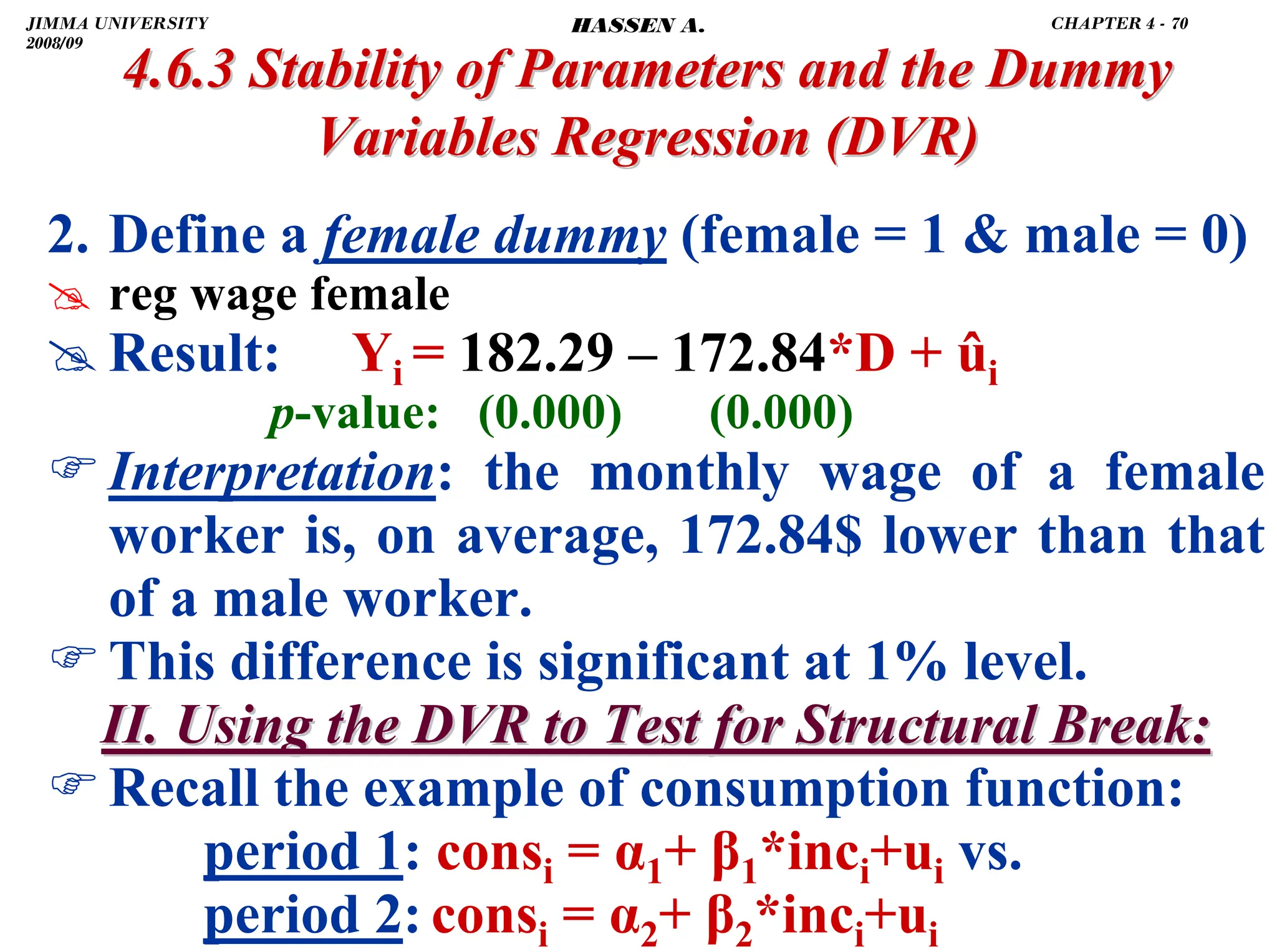
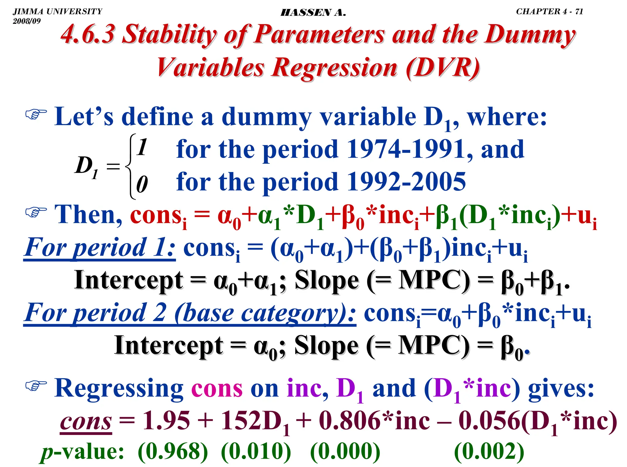
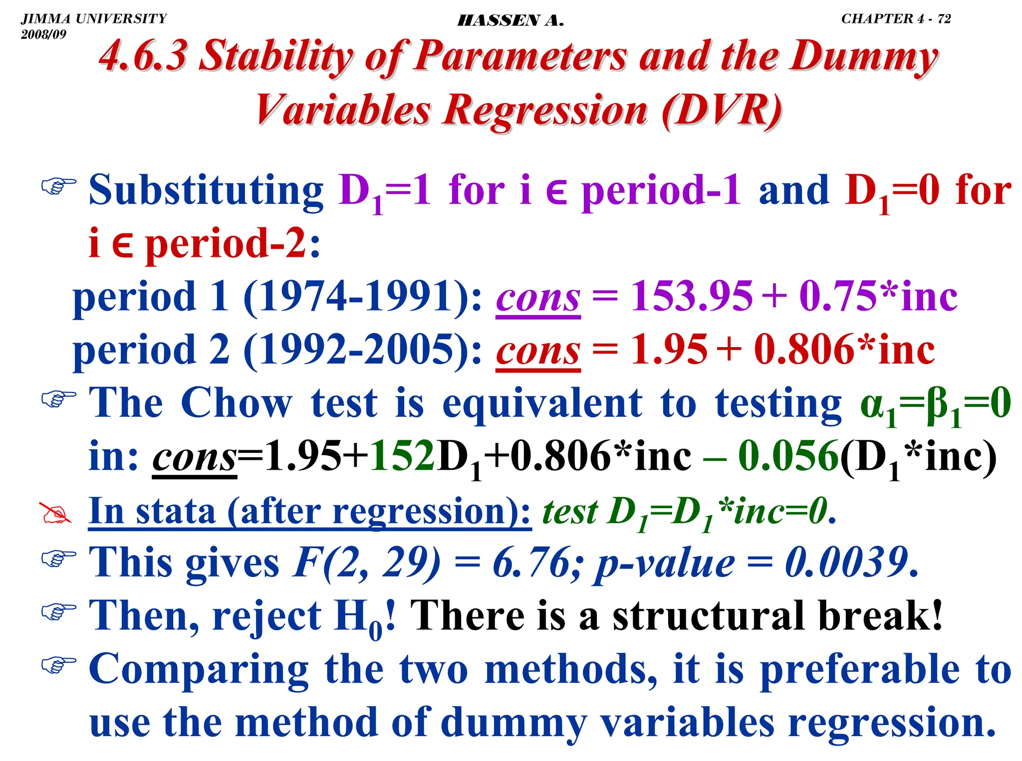
4.6.3 Stability of Parameters and the Dummy
4.6.3 Stability of Parameters and the Dummy
Variables Regression
Variables Regression (DVR)
(DVR)
2. Estimate the pooled/combined model (under
H0: no significant change/difference in β's).
)The RSS from this model is the RRSS with
n–(K+1) df; where n = n1+n2.
3. Then, under H0, the test statistic will be:
4. Find the critical value: FK+1,n-2(K+1) from table.
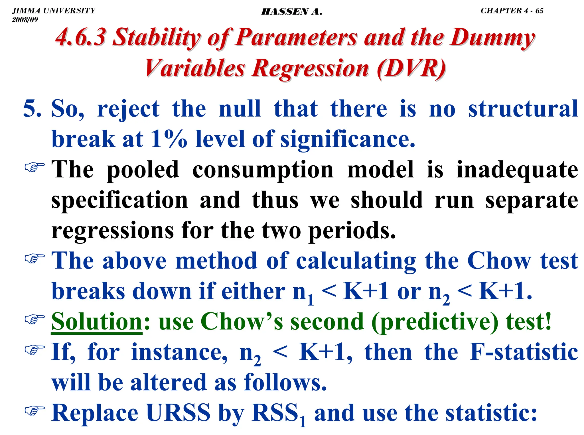
5. Reject the null of stable parameters (and favor
Ha: that there is structural break) if Fcal Ftab.
1)]
2(K
[n
URSS
1)
(K
URSS]
[RRSS
F
+
−
+
−
=
cal
JIMMA UNIVERSITY
2008/09
CHAPTER 4 - 62
HASSEN A.

217. .
4.6.3 Stability of Parameters and the Dummy
4.6.3 Stability of Parameters and the Dummy
Variables Regression
Variables Regression (DVR)
(DVR)
Example: Suppose we have the following results
from the OLS Estimation of real consumption
on real disposable income:
i. For the period 1974-1991: consi = α1+β1*inci+ui
Consumption = 153.95 + 0.75*Income
p-value: (0.000) (0.000)
RSS = 4340.26114; R2 = 0.9982
ii. For the period 1992-2005: consi = α2+ β2*inci+ui
Consumption = 1.95 + 0.806*Income
p-value: (0.975) (0.000)
RSS = 10706.2127; R2 = 0.9949
JIMMA UNIVERSITY
2008/09
CHAPTER 4 - 63
HASSEN A.

218. .
4.6.3 Stability of Parameters and the Dummy
4.6.3 Stability of Parameters and the Dummy
Variables Regression
Variables Regression (DVR)
(DVR)
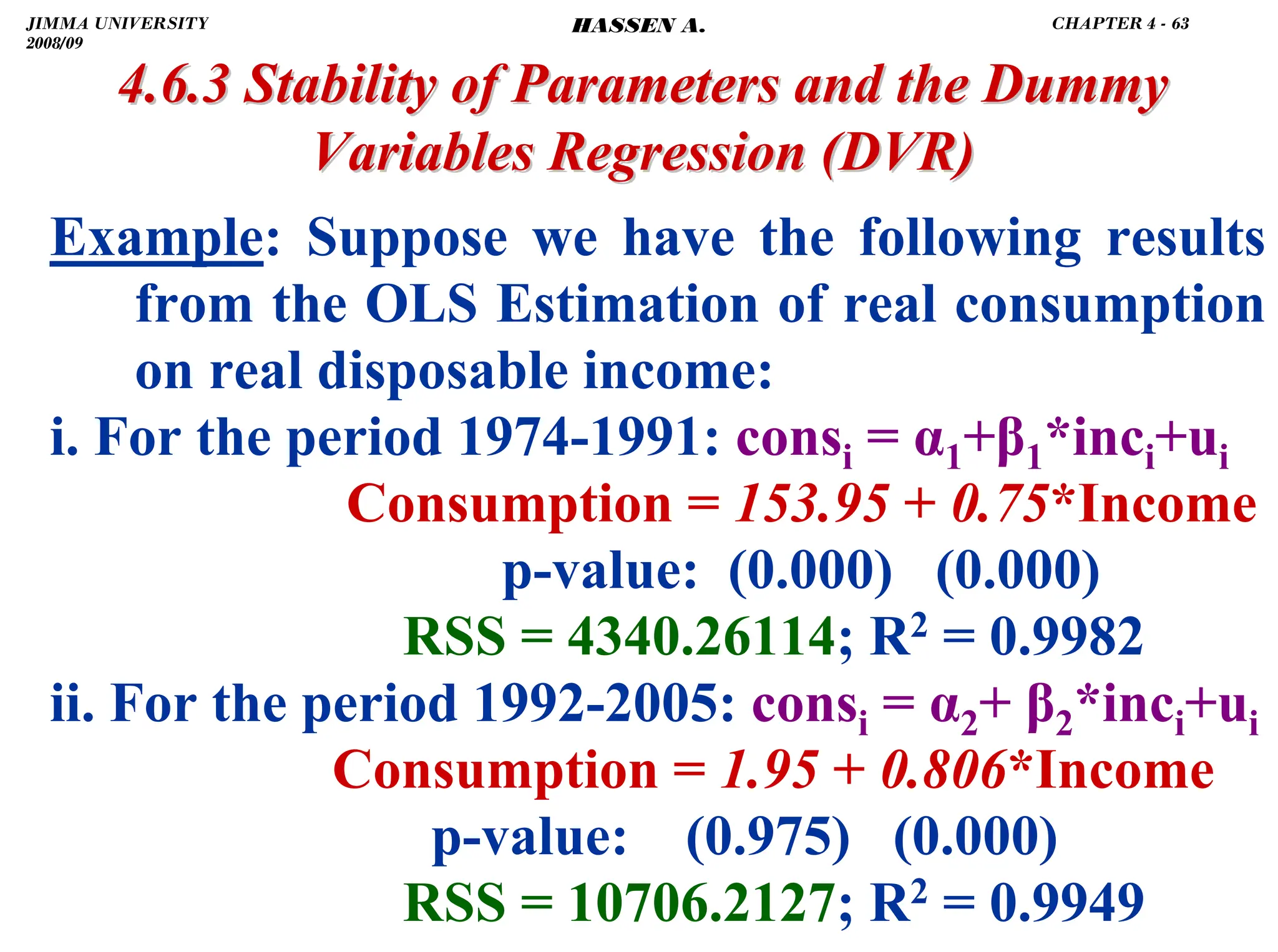
iii. For the period 1974-2005: consi = α+ β*inci+ui
Consumption = 77.64 + 0.79*Income
t-ratio: (4.96) (155.56)
RSS = 22064.6663; R2 = 0.9987
1. URSS = RSS1 + RSS2 = 15064.474
2. RRSS = 22064.6663
)K = 1 and K + 1 = 2; n1 = 18, n2 = 15, n = 33.
3. Thus,
4. p-value = Prob(F-tab 6.7632981) = 0.003883
6.7632981
29
15064.474
2
15064.474]
3
[22064.666
Fcal =
−
=
JIMMA UNIVERSITY
2008/09
CHAPTER 4 - 64
HASSEN A.

219. .
4.6.3 Stability of Parameters and the Dummy
4.6.3 Stability of Parameters and the Dummy
Variables Regression
Variables Regression (DVR)
(DVR)
5. So, reject the null that there is no structural
break at 1% level of significance.
)The pooled consumption model is inadequate
specification and thus we should run separate
regressions for the two periods.
)The above method of calculating the Chow test
breaks down if either n1 K+1 or n2 K+1.
)Solution: use Chow’s second (predictive) test!
)If, for instance, n2 K+1, then the F-statistic
will be altered as follows.
)Replace URSS by RSS1 and use the statistic:
JIMMA UNIVERSITY
2008/09
CHAPTER 4 - 65
HASSEN A.

220. .
4.6.3 Stability of Parameters and the Dummy
4.6.3 Stability of Parameters and the Dummy
Variables Regression
Variables Regression (DVR)
(DVR)
* The Chow test tells if the parameters differ on
average, but not which parameters differ.
* The Chow test requires that all groups have the
same error variance.
)This assumption is questionable: if parameters
can be different, then so can the variances be.
)One method of correcting for unequal error
variances is to use the dummy variable
approach with White's Robust Standard Errors.
1)
(K
n
RSS
n
]
RSS
[RRSS
F
1
1
2
1
cal
+
−
−
=
JIMMA UNIVERSITY
2008/09
CHAPTER 4 - 66
HASSEN A.

221. .
B. The Dummy Variables Regression
I. Introduction
I. Introduction:
:
# Not all information can easily be quantified.
) So, need to incorporate qualitative information.
e.g. 1. Effect of belonging to a certain group:
1 Gender, location, status, occupation
1 Beneficiary of a program/policy
2. Ordinal variables:
1 Answers to yes/no (or scaled) questions...
# Effect of some quantitative variable may differ
between groups/categories:
1 Returns to education may differ between
sexes or between ethnic groups …
4.6.3 Stability of Parameters and the Dummy
4.6.3 Stability of Parameters and the Dummy
Variables Regression
Variables Regression (DVR)
(DVR)
JIMMA UNIVERSITY
2008/09
CHAPTER 4 - 67
HASSEN A.

222. .
4.6.3 Stability of Parameters and the Dummy
4.6.3 Stability of Parameters and the Dummy
Variables Regression
Variables Regression (DVR)
(DVR)
# Interest in determinants of belonging to a group
1 Determinants of being poor …
)Dummy dependent variable (logit, probit…)
)Dummy Variable: a variable devised to use
qualitative information in regression analysis.
)A dummy variable takes 2 values: usually 0/1.
e.g. Yi=β0+β1*D+u; for i ϵ group 1, and
for i ∉ group 1.
¾If D = 0, E(Y) = E(Y|D = 0) = β0
¾If D = 1, E(Y) = E(Y|D = 1) = β0 + β1
)Thus, the difference between the two groups (in
mean values of Y) is: E(Y|D=1) – E(Y|D=0) = β1.
⎩
⎨
⎧
=
0
1
D
JIMMA UNIVERSITY
2008/09
CHAPTER 4 - 68
HASSEN A.

223. .
) So, the significance of the difference between
the groups is tested by a t-test of β1 = 0.
e.g.: Wage differential between male and female
) Two possible ways: a male or a female dummy.
1. Define a male dummy (male = 1 female = 0).
# reg wage male
# Result: Yi = 9.45 + 172.84*D + ûi
p-value: (0.000) (0.000)
) Interpretation: the monthly wage of a male
worker is, on average, 172.84$ higher than that
of a female worker.
) This difference is significant at 1% level.
4.6.3 Stability of Parameters and the Dummy
4.6.3 Stability of Parameters and the Dummy
Variables Regression
Variables Regression (DVR)
(DVR)
JIMMA UNIVERSITY
2008/09
CHAPTER 4 - 69
HASSEN A.

224. .
2. Define a female dummy (female = 1 male = 0)
# reg wage female
# Result: Yi = 182.29 – 172.84*D + ûi
p-value: (0.000) (0.000)
)Interpretation: the monthly wage of a female
worker is, on average, 172.84$ lower than that
of a male worker.
)This difference is significant at 1% level.
II. Using the DVR to Test for Structural Break:
II. Using the DVR to Test for Structural Break:
)Recall the example of consumption function:
period 1: consi = α1+ β1*inci+ui vs.
period 2: consi = α2+ β2*inci+ui
4.6.3 Stability of Parameters and the Dummy
4.6.3 Stability of Parameters and the Dummy
Variables Regression
Variables Regression (DVR)
(DVR)
JIMMA UNIVERSITY
2008/09
CHAPTER 4 - 70
HASSEN A.

225. .
) Let’s define a dummy variable D1, where:
for the period 1974-1991, and
for the period 1992-2005
) Then, consi = α0+α1*D1+β0*inci+β1(D1*inci)+ui
For period 1: consi = (α0+α1)+(β0+β1)inci+ui
Intercept =
Intercept = α
α0
0+
+α
α1
1; Slope (= MPC) =
; Slope (= MPC) = β
β0
0+
+β
β1
1.
For period 2 (base category): consi=α0+β0*inci+ui
Intercept =
Intercept = α
α0
0; Slope (= MPC) =
; Slope (= MPC) = β
β0
0.
.
) Regressing cons on inc, D1 and (D1*inc) gives:
cons = 1.95 + 152D1 + 0.806*inc – 0.056(D1*inc)
p-value: (0.968) (0.010) (0.000) (0.002)
4.6.3 Stability of Parameters and the Dummy
4.6.3 Stability of Parameters and the Dummy
Variables Regression
Variables Regression (DVR)
(DVR)
⎩
⎨
⎧
=
0
1
D1
JIMMA UNIVERSITY
2008/09
CHAPTER 4 - 71
HASSEN A.

226. .
) Substituting D1=1 for i ϵ period-1 and D1=0 for
i ϵ period-2:
period 1 (1974-1991): cons = 153.95 + 0.75*inc
period 2 (1992-2005): cons = 1.95 + 0.806*inc
) The Chow test is equivalent to testing α1=β1=0
in: cons=1.95+152D1+0.806*inc – 0.056(D1*inc)
# In stata (after regression): test D1=D1*inc=0.
) This gives F(2, 29) = 6.76; p-value = 0.0039.
) Then, reject H0! There is a structural break!
) Comparing the two methods, it is preferable to
use the method of dummy variables regression.
4.6.3 Stability of Parameters and the Dummy
4.6.3 Stability of Parameters and the Dummy
Variables Regression
Variables Regression (DVR)
(DVR)
JIMMA UNIVERSITY
2008/09
CHAPTER 4 - 72
HASSEN A.

227. .
)This is because with the method of DVR:
1. we run only one regression.
2. we can test whether the change is in the
intercept only, in the slope only, or in both.
In our example, the change is in both. Why???
)For a total of m categories, use m–1 dummies!
)Including m dummies (1 for each group) results
in perfect multicollinearity (the dummy
variable trap). e.g.: 2 groups 2 dummies:
)constant = D1 + D2 !!!
4.6.3 Stability of Parameters and the Dummy
4.6.3 Stability of Parameters and the Dummy
Variables Regression
Variables Regression (DVR)
(DVR)
⎥
⎥
⎥
⎦
⎤
⎢
⎢
⎢
⎣
⎡
=
1
0
X
1
0
1
X
1
0
1
X
1
X
13
12
11
]
D
D
[constant
X 2
1
=
JIMMA UNIVERSITY
2008/09
CHAPTER 4 - 73
HASSEN A.

228. .
)Simultaneity occurs when an equation is part of
a simultaneous equations system, such that
causation runs from Y to X as well as X to Y.
)In such a case, cov(X,ε) ≠ 0 and OLS estimators
are biased and inconsistent.
)Such situations are pervasive in economic
models so simultaneity bias is a vital issue.
e.g. The Simple Keynesian Consumption Function
)Structural form model: consists of the national
accounts identity and a basic consumption
function, i.e., a pair of simultaneous equations.
4.6.4 Simultaneity Bias
4.6.4 Simultaneity Bias
JIMMA UNIVERSITY
2008/09
CHAPTER 4 - 74
HASSEN A.

229. .
)Yt Ct are endogenous (simultaneously
determined) and It is exogenous.
)Reduced form: expresses each endogenous
variable as a function of exogenous variables,
(and/or predetermined variables – lagged
endogenous variables, if present) and random
error term/s.
)The reduced form is:
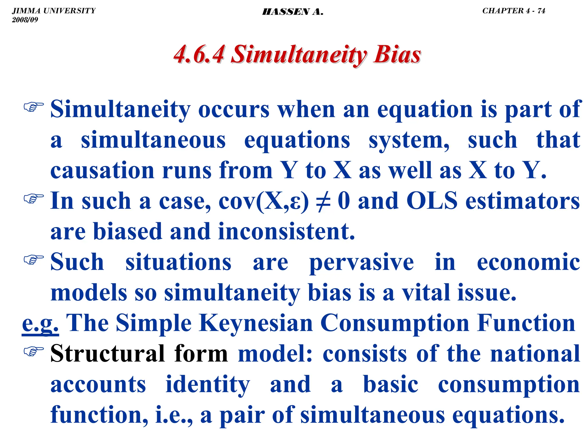
4.6.4 Simultaneity Bias
4.6.4 Simultaneity Bias
⎪
⎪
⎩
⎪
⎪
⎨
⎧
+
+
−
=
+
+
−
=
]
t
U
t
βI
)[α
β
1
1
(
t
C
]
t
U
t
I
)[α
β
1
1
(
t
Y
⎩
⎨
⎧
+
+
=
+
=
t
t
t
t
t
t
U
βY
α
C
I
C
Y
JIMMA UNIVERSITY
2008/09
CHAPTER 4 - 75
HASSEN A.

230. .
)The reduced form equation for Yt shows that:
)Yt, in Ct = α + βYt + Ut, is correlated with Ut.
)OLS estimators for β (MPC) α (autonomous
consumption) are biased and inconsistent.
)
) Solution
Solution: IV/2SLS
4.6.4 Simultaneity Bias
4.6.4 Simultaneity Bias
]
U
),
U
I
)(α
β
1
1
cov[(
)
U
,
cov(Y t
t
t
t
t +
+
−
=
)]
U
,
U
cov(
)
U
,
I
cov(
)
U
,
)[cov(α
β
1
1
( t
t
t
t
t +
+
−
=
0
)
β
1
(
)
)var(U
β
1
1
( t ≠
−
=
−
=
2
U
σ
JIMMA UNIVERSITY
2008/09
CHAPTER 4 - 76
HASSEN A.

231. .
… THE END …
GOOD LUCK!
GOOD LUCK!
JIMMA UNIVERSITY
2008/09
CHAPTER 4 - 77
HASSEN A.