The document describes the mathematical modeling of a three-phase transformer connected in a delta-grounded wye configuration. It presents the voltage and current relationships between the primary delta and secondary wye windings using matrix notation. The derivation shows how to relate the line-to-line voltages on the primary side to the equivalent line-to-neutral voltages on the secondary side.

1. E

2. Three Phase Transformer Models
• For a four wire system, the most common connection is
(delta – grounded wye). ∴ We will look at this transformer.
Convention
• Above gives the voltages and currents for any transformer bank
connected between source node n and load node m.

3. • Capitals refer to source (node n) whilst common
letters refer to load (node m).
• It is assumed that connections are to the “American
Standard 30°” connection such that:
For Step-Down connection:
VAB leads Vab by 30° … (1)
IA leads Ia by 30° … (2)
For Step-Up connection:
Vab leads VAB by 30° … (3)
Ia leads IA by 30° … (4)

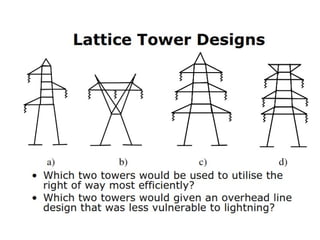
4. Generalized Matrices:
[VLNABC] = [at] [VLNabc] + [bt] [Iabc] … (5)
[IABC] = [ct] [VLNabc] + [dt][Iabc] … (6)
Also, we can write:
[VLNabc] = [At] [VLNABC] – [Bt] [Iabc] … (7)
These represent the line to neutral voltages for an
ungrounded wye connection or line ground voltages for
a grounded wye connection.
For a delta connection, the voltage matrices represent
“equivalent” line to neutral voltages.

5. The Delta/Grounded Wye Step Down
Connection ( )
Note that Vta is 180° out of phase with VCA
Vtb “ “ “ “ VAB
Vtc “ “ “ “ VBC

6. ∴ Vab = Vta – Vtb … (8)
For the transformer: nt = VLLrated … (9)
Vlnrated
where VLL = rated high voltage
∴ VLn = rated low side = Vt
|VLL| = nt|Vt| … (10)
But equivalent +ve sequence line to neutral voltage on delta side is:
|VLN| = |VLL|/√3
Or |VLN| = nt|Vt| = at |Vt| … (11)
√3
where at = nt = VLL
∴ √3 √3VLn
∴at = VLL(rated HV side) … (12)
Vll(rated LV side)
VAB  0 − the 0
Takinginto account nt 180°shiftVta  can write the following equations:
 we
∴ V  =  0
 BC   0 − n  = V  … (13)
t  tb 
VCA 
  − nt
 0 0 
 Vtc 
 

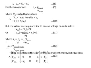
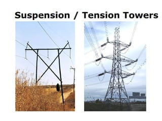
7. Or in compact form: [VLLABC] = [AV] [Vtabc] … (14)
 0 − nt 0 
where [ AV ] =  0
 0 − nt 

… (15)
− nt
 0 0  
Equation (14) gives the primary line to line voltages at Node ‘n’ as functions of
ideal voltages. What we need is a relationship between the equivalent line to
neutral voltage at node ‘n’ and the ideal secondary voltages. How to determine
the equivalent LV voltages?
Apply the Theory of Symmetrical Components:
[VLL012] = [T.]-1 [VLLABC] … (16)
1 1 1
where T = 1 as2
 as 

… (17)
1 as
 as 
2

where as = 1∠120
By definition, the zero sequence line-line voltage is always zero. The
relationship between +ve and –ve sequence line to line and line to neutral
voltages is known.

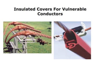
8. Hence:
VLN 0  1 0 0  VLL0 
   
VLN1  = 0 t s 0  VLL1 
* … (18)
  
VLN  0 0 t s  VLL 
 2   2 
ts = 1/√3 ∠ 30
Or in compact form: [VLN012] = [S] [VLL102] … (19)
where … (20)
Since VLL0 = 0 , then S[1,1] can be any value. We choose 1 for ease of manipulation.
The equivalent line to neutral voltages as functions of sequence line to neutral voltages are:
[VLNABC] = [T] [VLN012] … (21)
Sub (19) into (21) yields:
[VLNABC] = [T] [S] [VLL012] … (22)
Sub (16) into (22):
[VLNABC] = [T] [S] [T]-1[VLLABC] … (23)
Or [VLNABC] = [W] [VLLABC] 2 1 0 … (23)
1
0 2 1
3 
where [W] = [T] [S] [T]-1 = 1 0 2 
  … (24)
Equation (23) gives a way of calculating the equivalent LN voltages from a knowledge of the
LL voltages.

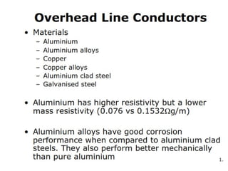
9. Sub (14) into (23)
[VLNABC] = [W] [AV] [Vtabc] = [at] [Vtabc] … (25)
0 2 1 
− nt 
where [at] = [W] [AV] = 1 0 2 … (26)
3  
2 1 0
 
Equation (25) defines the generalized [a] matrix for the delta-grounded
wye ( ) step down connection.
The ideal secondary voltages as functions of the secondary line to ground
voltages and secondary line currents are:
[Vtabc] = [VLGabc] + [Ztabc] [Iabc] … (27)
Z t a 0 0 
[
where Z t abc =  0] 
Z tb 0 
 … (28)
0 0 Z tc 
 
where Zta, Ztb, Ztc can be any value (May not be equal)

10. Sub (27) into (25):
[VLNABC] = [at]([VLGabc] + [Ztabc][Iabc]) … (29)
[VLNABC] = [at][VLGabc] + [bt][Iabc] … (30)
where [bt] = [at] [Ztabc]
 0 2 Ztb Ztc 
− nt 
Zta 0 2 Ztc 
Or [bt] = 3  
2 Zta Ztb
 0  
From (14) [ Vtabc] = [ AV ]-1 [ VLL ABC ] …(31)
Also [ VLL ABC ] = [ D ] [ V LN ABC] …(32)
1 −1 0
0 1 −1
 
Where [D] = −1 0 1 …(33)
 

11. Subs. (32) into (31) yields:
[Vtabc] = [AV]-1. [D]. [VLNABC] = [At].[VLNABC] … (34)
 1 0 − 1
where [At] = [AV] . [D] =
-1
1 … (35)
−1 1 0 
nt  
 0 −1 1 
 
Sub. (27) into (34)
[VLGabc] + [Ztabc][Iabc] = [At] . [VLNABC] … (36)
Rearranging:
[VLGabc] = [At] [VLNABC] – [Bt] [Iabc] … (37)
Z t a 0 0 
 
0 Z tb 0 
where [Bt] = [Ztabc] =  0
 0 Z tc 
 … (38)

12. Currents in Connection
From the diagram before, the 30° connection implies IA1
leads Ia1 by 30° or the +ve sequence current. Also Ia1 is in
phase with IAC1 (from the diagram).

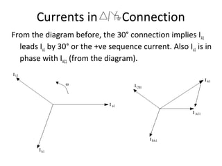
13. From Kirchhoff’s current Law:
 I A   1 − 1 0   I AC 
 I  =  0 1 − 1  
 B    I BA  … (39)
 I C  − 1 0 1   I 
     CB 
Or [IABC] = [D] [I∆ABC] … (40)
where I∆ ≡ current in each delta winding
The matrix equation relating ∆ primary to the secondary line currents is given by:
 I AC   1 0 0  I a 
 I  = 1  0 1 0  I 
 BA  nt   b  … (41)
 I CB 
   0 0 1  I c 
  
Or [I∆ABC] = [AI] [Iabc] … (42)
Sub (42) into (40)
[IABC] = [D] [AI] [Iabc] = [ct] [VLGabc] + [dt] [Iabc] … (43)
 1 −1 0 
1
where [dt] = [D] [AI] = n  0 1 − 1  … (44)
t
− 1 0 1 
 
And [ct] = [0] … (45)
Equation (43) gives the line currents (Node n) knowing the line currents at node m.

14. Example:
In the Example System of Figure A an unbalanced constant impedance load is
being served at the end of a one-mile section of a three-phase line. The line is
grounded wye with a per-unit impedance of 0.085 ∠85. The phase conductors of
being fed from a substation transformer rated 5000kVA, 138kV delta- 12.47kV
the line are 336,400 26/7 ACSR with a neutral conductor 4/0 ACSR. The
configuration and computation of the phase impedance matrix is give.
 0.4576 + j1.0780 0.1560 + j 0.5017 0.1535 + j 0.3849
[ Z lineabc ] = 0.1560 + j 0.5017 0.4666 + j1.0482 0.1580 + j 0.4236 Ω / mile
 
0.1535 + j 0.3849 0.1580 + j 0.4236 0.4615 + j1.0651 
 

15. The transformer impedance needs to be converted to per-unit referenced to the
low-voltage side of the transformer. The base impedance is
Zbase = 12.472 . 1000 = 31.1
5000
The transformer impedance referenced to the low-voltage side is
Zt = (0.085∠ 85) . 31.3 = 0.2304 + j2.6335 Ω
The transformer phase impedance matrix is
0.2304 + j 2.6335 0 0 
[ Ztabc ] = 
 0 0.2304 + j 2.6335 0 Ω


 0 0 0.2304 + j 2.6335

The unbalanced constant impedance load is connected in grounded wye. The load
impedance matrix is specified to be
 +6 j
12 0 0 
[ Zload abc ] =  0
 13 + j 4 0 Ω

 0
 0 14 + j 5

The unbalanced line-to-line voltages at Node 1 serving the substation transformer
are given as:  138,000∠0 
[VLLABC ] = 135,500∠ − 115.5 V
 
 145,959∠123.1 
 

16. 1. Determine the generalized matrices for the transformer.
The transformer turns ratio is nt = kVLLhigh = 138 = 19.1678
kVLNlow 12.47/√3
The transformer ratio is at = kVLLhigh = 138 = 11.0666
kVLLlow 12.47
From Equation 8.26:
0 2 1  0 −12.7786 − 6.3893 
[ at ] = −19.1678 .1
 0 2 =  − 6.3893
  0 −12.7786
3
2
 1 0 −12.7786
  − 6.3893 0 

From Equation 30:
 0 2.(0.2304 + j 2.6335) (0.2304 + j 2.6335) 
− 19.1678 
[ bt ] = . (0.2304 + j 2.6335) 0 2.(0.2304 + j 2.6335)

3
2.(0.2304 + j 2.6335) (0.2304 + j 2.6335)
 0 

 0 − 2.9441 − j 33.6518 −1.4721 − j16.8259 
[bt ] =  −1.4721 − j16.8259
 0 − 2.9441 − j 33.6518

− 2.9441 − j 33.6518
 −1.4721 − j16.8259 0 


17. From Equation 44:
 1 − 1 0   0.0522 − 0.0522 0 
1
[d t ] = . 0 1 − 1 =  0 0.0522 − 0.0522
19.1678    
− 1 0 1  − 0.0522
   0 0.0522 

From Equation 35:
 1 0 − 1  0.0522 0 − 0.0522
1
[ At ] = .− 1 1 0  = − 0.0522 0.0522
   0 

19.1678
 0 −1 1   0
   − 0.0522 0.0522 
From Equation 38:
0.2304 + j 2.6335 0 0 

[ Bt ] = [ Zt abc ] =  0 0.2304 + j 2.6335 0 


 0 0 0.2304 + j 2.6335

2.Given the line-to-line voltages at Node 1, determine the ideal transformer
voltages. From Equation 15:
 0 − nt 0   0 − 19.1678 0 
[ AV ] =  0
 0 =
− nt   0 0 − 19.1678

− nt
 0 0  −19.1678
  0 0 

7614.8∠ − 56.9
[Vt abc ] = [ AV ]−1.[VLL ABC ] =  7199.6∠
 180  V

 7069∠64.5 
 

18. 3. Determine the load currents.
Kirchhoff’s voltage law gives:
[Vtabc] = ([Ztabc] + [Zlineabc] + [Zloadabc]). [Iabc] = [Ztotalabc] . [Iabc]
12.688 + j 9.7115 0.156 + j 0.5017 0.1535 + j 0.3849 
[ Ztotalabc ] =  0.156 + j 0.5017 13.697 + j 7.6817 0.158 + j 0.4236  Ω
 
0.1535 + j 0.3849 0.158 + j 0.4236 14.6919 + j8.6986
 
The line currents can now be computed:
484.1∠ − 93.0
[ I abc ] = [ Ztotal abc ]−1.[Vt abc ] =  470.7∠151.5  A
 
 425.4∠34.8 
 
4. Determine the line-to-ground voltages at the load and at Node 2.
6494.8∠ − 66.4
[Vload abc ] = [ Ztotal abc ].[ I abc ] =  6401.6∠171.0  V
 
 6323.5∠54.4 
 
6842.2∠ − 65.0
[VLGabc ] = [Vload abc ] + [ Zlineabc ].[ I abc ] =  6594.5∠171.0  V
 
 6594.9∠56.3 
 

19. 5. Using the generalized matrices, determine the equivalent line-to-
neutral voltages and the line-to-line voltages at Node 1.
 83,224∠ − 29.3 
[VLN ABC ] = [at ].[VLGabc ] + [bt ].[ I abc ] = 77,103∠ − 148.1 V
 
 81,843∠95.0 
 
 138,000∠0 
[VLLABC ] = [ D].[VLN ABC ] = 135,500∠ − 148.1 V
 
 145,959∠123.1 
 
It is always comforting to be able to work back and compute what was
initially given. In this case, the line-to-line voltages at Node 1 have
been computed and the same values result that were given at the
start of the problem.

20. 6. Use the reverse equation to verify that the line-to-ground voltages
at Node 2 can be computed knowing the equivalent line-to-neutral
voltages at Node 1 and the currents leaving Node 2.
6842.2∠ − 65.0
[VLGabc ] = [ At ].[VLN ABC ] − [ Bt ].[ I abc ] =  6594.5∠171.0  V
 
 6494.9∠56.3 
 
These are the same values for the line-to-ground voltages at Node 2
that were determined working from the load towards the source.
This Example has demonstrated the application of the generalized
constants. The example also provides verification that the same
voltages and currents result when working from the load toward
the source or from the source toward the load.

29. Interconnection
to Other Utilities

36. Disconnect Switches

37. Disconnect Switch

39. Circuit Breakers

40. Lightning Arrester

41. Reclosures
Manual Automatic

42. Capacitor Banks

43. Protection Equipment

44. Meter Loop
Service Drop Conductors

45. Ground wire/Ground Rod
Meter Enclosure
Service Mast