This document discusses digital implementation of analog controllers. There are three main approaches to digitizing an analog controller: 1) emulation using the forward rectangular rule to approximate derivatives with differences, 2) emulation using the backward rectangular rule, and 3) emulation using the bilinear rule. The zero-order hold operation in the digital to analog conversion introduces an effective delay that degrades the emulated system's performance compared to the original analog controller. Faster sampling reduces the impact of this delay.

1. ECE4510/5510: Feedback Control Systems. 10–1
DIGITAL CONTROLLER IMPLEMENTATION
10.1: Some background in digital control
■ We can implement our controllers with op-amp circuits (cf. Chap. 7).
■ More commonly nowadays, we use digital computers (e.g.,
microcontrollers) to implement our control designs.
■ There are two main approaches to digital controller design:
1. Emulation of an analog controller—we look at this here.
2. Direct digital design—subject of more advanced course.
■ Emulation is when a digital computer approximates an analog
controller design.
ANALOG:
D(s) G(s) y(t)r(t)
u(t)e(t)
DIGITAL:
zoh
D2AA2D
D(z) G(s)Q y(t)r(t)
u(t)u(kT)e(t) e(kT )
■ Analog controller computes u(t) from e(t) using differential equations.
For example,
˙u(t) + bu(t) = k0 ˙e(t) + ak0e(t).
Lecture notes prepared by and copyright c⃝ 1998–2013, Gregory L. Plett and M. Scott Trimboli

2. ECE4510/ECE5510, DIGITAL CONTROLLER IMPLEMENTATION 10–2
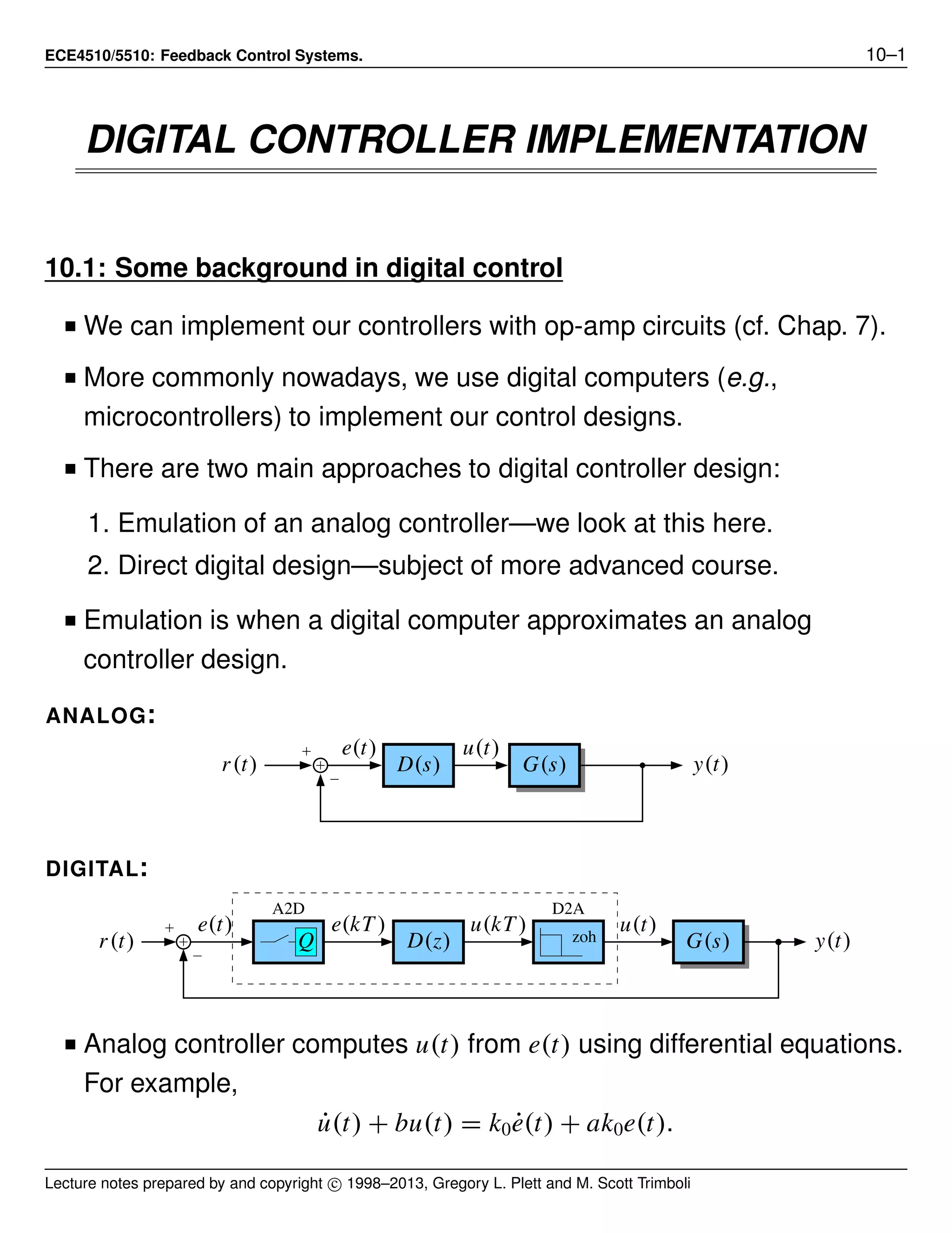
■ Digital controller computes u(kT) from e(kT) using difference
equations. For example (we’ll see where this came from shortly),
u(kT) = (1 − bT)u((k − 1)T) + k0(aT − 1)e((k − 1)T) + k0e(kT).
■ To interface the computer controller to the “real world” we need an
analog-to-digital converter (to measure analog signals) and
digital-to-analog converter (to output signals).
■ Sampling and outputting usually done synchronously, at a constant
rate. If sampling period = T , frequency = 1/T .
■ The signals inside the computer (the sampled signals) are noted as
y(kT), or simply y [k]. y [k] is a discrete-time signal, where y(t) is a
continuous-time signal.
y(t) y(kT) = y[k]
■ So, we can write the prior difference equation as
u[k] = (1 − bT)u[k − 1] + k0(aT − 1)e[k − 1] + k0e[k].
■ Discrete-time signals are usually converted to continuous-time
signals using a zero-order hold:
e.g., to convert u [k] to u(t).
Efficient implementation
■ We look at some efficient pseudo-code for an implementation of
u[k] = (1 − bT)u[k − 1] + k0(aT − 1)e[k − 1] + k0e[k].
Lecture notes prepared by and copyright c⃝ 1998–2013, Gregory L. Plett and M. Scott Trimboli

3. ECE4510/ECE5510, DIGITAL CONTROLLER IMPLEMENTATION 10–3
■ Output of digital controller u[k] depends on previous output u[k − 1]
as well as the previous and current errors e[k − 1] and e[k].
Real-Time Controller Implementation
x = 0. (initialization of “past” values for first loop through)
Define constants:
α1 = 1 − bT .
α2 = k0(aT − 1).
READ A/D to obtain y[k] and r[k].
e[k] = r[k] − y[k].
u[k] = x + k0e[k].
OUTPUT u[k] to D/A and ZOH.
Now compute x for the next loop through:
x = α1u[k] + α2e[k].
Go back to “READ” when T seconds have elapsed since last READ.
■ Code is optimized to minimize latency between A2D read and D2A
write.
R = read. W = write.
C = compute. I = idle.
RRR CCC WWW III
T
Lecture notes prepared by and copyright c⃝ 1998–2013, Gregory L. Plett and M. Scott Trimboli

4. ECE4510/ECE5510, DIGITAL CONTROLLER IMPLEMENTATION 10–4
10.2: “Digitization” (emulation of analog controllers)
■ Continuous-time controllers are designed with Laplace-transform
techniques. The resulting controller is a function of “s”.
y(t) =
dx(t)
dt
x(t) s
■ So, “s” is a derivative operator. There are several ways of
approximating this in discrete time.
Forward-rectangular rule
■ We first look at the “forward rectangular” rule. We write:
˙x(t)
△
= lim
δt→0
δx(t)
δt
= lim
δt→0
x(t + δt) − x(t)
δt
.
■ If sampling interval T = tk+1 − tk is small,1
˙x(kT) ≈
x((k + 1)T) − x(kT)
T
i.e., ˙x[k] ≈
x[k + 1] − x[k]
T
.
Backward-rectangular rule
■ We could also write ˙x(t)
△
= lim
δt→0
δx(t)
δt
= lim
δt→0
x(t) − x(t − δt)
δt
.
■ Then, if T is small,
˙x(kT) ≈
x(T) − x((k − 1)T)
T
i.e., ˙x[k] ≈
x[k] − x[k − 1]
T
.
Bilinear (or Tustin) rule
■ We could also re-index the forward-rectangular rule as
˙x[k − 1] =
x[k] − x[k − 1]
T
to have the same right-hand-side as the backward-rectangular rule.
1
Rule of thumb: Sampling frequency must be ≈ 30 times the bandwidth of the analog
system being emulated for comparable performance.
Lecture notes prepared by and copyright c⃝ 1998–2013, Gregory L. Plett and M. Scott Trimboli

5. ECE4510/ECE5510, DIGITAL CONTROLLER IMPLEMENTATION 10–5
■ Then, we average these two forms:
˙x[k] + ˙x[k − 1]
2
=
x[k] − x[k − 1]
T
.
Digitizing a controller
■ Once we’ve chosen which rule to use, we “digitize” controller D(s) by
1. Writing U(s) = D(s)E(s).
2. Converting to differential equation:
n
k=0
ak
dk
u(t)
dtk
=
m
k=0
bk
dk
e(t)
dtk
.
3. Replacing derivatives with differences.
EXAMPLE: Digitize the lead or lag controller D(s) =
U(s)
E(s)
= k0
s + a
s + b
using
the forward-rectangular rule.
1. We write
U(s) = k0
s + a
s + b
E(s)
(s + b)U(s) = k0(s + a)E(s)
2. We take the inverse-Laplace transform of this result, term-by-term to
get
˙u(t) + bu(t) = k0 ˙e(t) + ak0e(t).
3. Use “forward-rectangular rule” to digitize
u[k + 1] − u[k]
T
+ bu[k] = k0
e[k + 1] − e[k]
T
+ ae[k]
u[k + 1] = u[k] +
T −bu[k] + k0
e[k + 1] − e[k]
T
+ ae[k]
= (1 − bT )u[k] + k0(aT − 1)e[k] + k0e[k + 1],
Lecture notes prepared by and copyright c⃝ 1998–2013, Gregory L. Plett and M. Scott Trimboli

6. ECE4510/ECE5510, DIGITAL CONTROLLER IMPLEMENTATION 10–6
or,
u[k] = (1 − bT)u[k − 1] + k0(aT − 1)e[k − 1] + k0e[k].
■ This is how we got the result at the beginning of this chapter of notes.
EXAMPLE: Digitize the lead or lag controller D(s) =
U(s)
E(s)
= k0
s + a
s + b
using
the backward-rectangular rule.
1. As before, we have
(s + b)U(s) = k0(s + a)E(s).
2. Again, we have
˙u(t) + bu(t) = k0 ˙e(t) + ak0e(t).
3. Use “backward-rectangular rule” to digitize
u[k] − u[k−1]
T
+ bu[k] = k0
e[k] − e[k−1]
T
+ ae[k]
u[k] = u[k−1] +
T −bu[k] + k0
e[k] − e[k−1]
T
+ ae[k]
(1 + bT) u[k] = u[k−1] + k0(aT + 1)e[k] − k0e[k−1]
u[k] =
1
1 + bT
(u[k−1] + k0(aT + 1)e[k] − k0e[k−1]) .
■ Notice that this is a different result from before.
EXAMPLE: Digitize the lead or lag controller D(s) =
U(s)
E(s)
= k0
s + a
s + b
using
the bilinear rule.
1. As before, we have (s + b)U(s) = k0(s + a)E(s).
2. Again, we have ˙u(t) + bu(t) = k0 ˙e(t) + ak0e(t).
Lecture notes prepared by and copyright c⃝ 1998–2013, Gregory L. Plett and M. Scott Trimboli

7. ECE4510/ECE5510, DIGITAL CONTROLLER IMPLEMENTATION 10–7
3. Using the bilinear rule is challenging since we need to have
derivatives in a specific format. We’ll use a trick here (ECE4540/5540
teaches more advanced techniques that don’t need this trick).
■ Re-index the differential equation:
˙u(t − T ) + bu(t − T ) = k0 ˙e(t − T ) + ak0e(t − T ).
■ Add this to the prior version, and divide by 2
˙u(t) + ˙u(t−T )
2
+ b
u(t) + u(t−T )
2
= k0
˙e(t) + ˙e(t−T)
2
+ ak0
e(t) + e(t−T )
2
u[k] − u[k−1]
T
+
b
2
[u[k] + u[k−1]] = k0
e[k] − e[k−1]
T
+
ak0
2
[e[k] + e[k−1]] .
■ Rearranging,
1 +
bT
2
u[k] = 1 −
bT
2
u[k−1] + k0 1 +
aT
2
e[k]
− k0 1 −
aT
2
e[k−1]
u[k] =
2 − bT
2 + bT
u[k−1] + k0
2 + aT
2 + bT
e[k] − k0
2 − aT
2 + aT
e[k−1].
■ Again, this is a different result from before.
Lecture notes prepared by and copyright c⃝ 1998–2013, Gregory L. Plett and M. Scott Trimboli

8. ECE4510/ECE5510, DIGITAL CONTROLLER IMPLEMENTATION 10–8
10.3: The impact of the zero-order hold
■ We illustrate the results of the prior three examples by substituting
numeric values.
■ Let D(s) = 70
(s + 2)
(s + 10)
, G(s) =
1
s(s + 1)
.
■ Choose to try a sample rate of 20 Hz and also try 40 Hz.
(Note, BW of analog system is ≈ 1Hz or so).
FORWARD-RECTANGULAR RULE: Digitizing D(s) gives
■ 20 Hz: u[k + 1] = 0.5u[k] + 70e[k + 1] − 63e[k].
■ 40 Hz: u[k + 1] = 0.75u[k] + 70e[k + 1] − 66.5e[k].
BACKWARD-RECTANGULAR RULE: Digitizing D(s) gives
■ 20 Hz: u[k + 1] = 0.6666u[k] + 51.3333e[k + 1] − 46.6666e[k].
■ 40 Hz: u[k + 1] = 0.8u[k] + 58.8e[k + 1] − 56e[k].
BILINEAR RULE: Digitizing D(s) gives
■ 20 Hz: u[k + 1] = 0.6u[k] + 58.8e[k + 1] − 53.2e[k].
■ 40 Hz: u[k + 1] = 0.7778u[k] + 63.7777e[k + 1] − 60.666e[k].
0 0.2 0.4 0.6 0.8 1
0
0.5
1
1.5
analog
forward
backward
bilinear
Time (sec)
Plantoutput
Sampled at 20Hz
0 0.2 0.4 0.6 0.8 1
0
0.5
1
1.5
analog
forward
backward
bilinear
Time (sec)
Plantoutput
Sampled at 40Hz
■ IMPORTANT NOTE: The digitized system has poorer damping than
the original analog system. This will always be true when emulating
an analog controller. We see why next . . .
Lecture notes prepared by and copyright c⃝ 1998–2013, Gregory L. Plett and M. Scott Trimboli

9. ECE4510/ECE5510, DIGITAL CONTROLLER IMPLEMENTATION 10–9
The D2A “Hold” Operation
u(t)
avg. u(t)
u(kT)u
■ Even if u(kT) is a perfect re-creation of the output of the analog
controller at t = kT, the “hold” in the D2A causes an “effective delay.”
■ The delay is approximately equal to half of the sampling period: T/2.
■ Recall from frequency-response analysis and design, the magnitude
of a delayed response stays the same, but the phase changes:
phase = −ω
T
2
.
■ For the previous example, sampling now at 10Hz, we have:
10
−1
10
0
10
1
10
2
10
−1
10
0
10
1
10
−1
10
0
10
1
10
2
−180
−160
−140
−120
−100
Frequency (rad/sec)
MagnitudePhase(Deg)
■ The PM has changed from ≈ 50◦
to ≈ 30◦
.
■ ζ ≈
PM
100
. . . ζ changed from 0.5 to 0.3 . . . much less damping.
Lecture notes prepared by and copyright c⃝ 1998–2013, Gregory L. Plett and M. Scott Trimboli

10. ECE4510/ECE5510, DIGITAL CONTROLLER IMPLEMENTATION 10–10
■ Mp from about 20% to
about 30% . . .
■ Faster sampling. . .
smaller T . . . smaller
delay. . . smaller
change in response. 0 0.2 0.4 0.6 0.8 1
0
0.5
1
1.5
Time (sec)
Plantoutput
Root-Locus View of the Delay
■ Recall that we can model a delay using a Padé approximation.
■
T
2
delay −→ e−sT/2
≈
1 − sT/4
1 + sT/4
.
■ Poles and zeros reflected about the jω-axis.
−
4
T
4
T
I(s)
R(s)
As T → 0, delay dynamics → ∞.
■ Impact of delay: Suppose D(s)G(s) =
1
s + a
.
−a
I(s)
R(s)
With
delay
➠ −
4
T
4
T
−a
I(s)
R(s)
■ Does the delayed locus make sense?
1 − sT/4
1 + sT/4
= −
(sT/4 − 1)
(sT/4 + 1)
.
Lecture notes prepared by and copyright c⃝ 1998–2013, Gregory L. Plett and M. Scott Trimboli

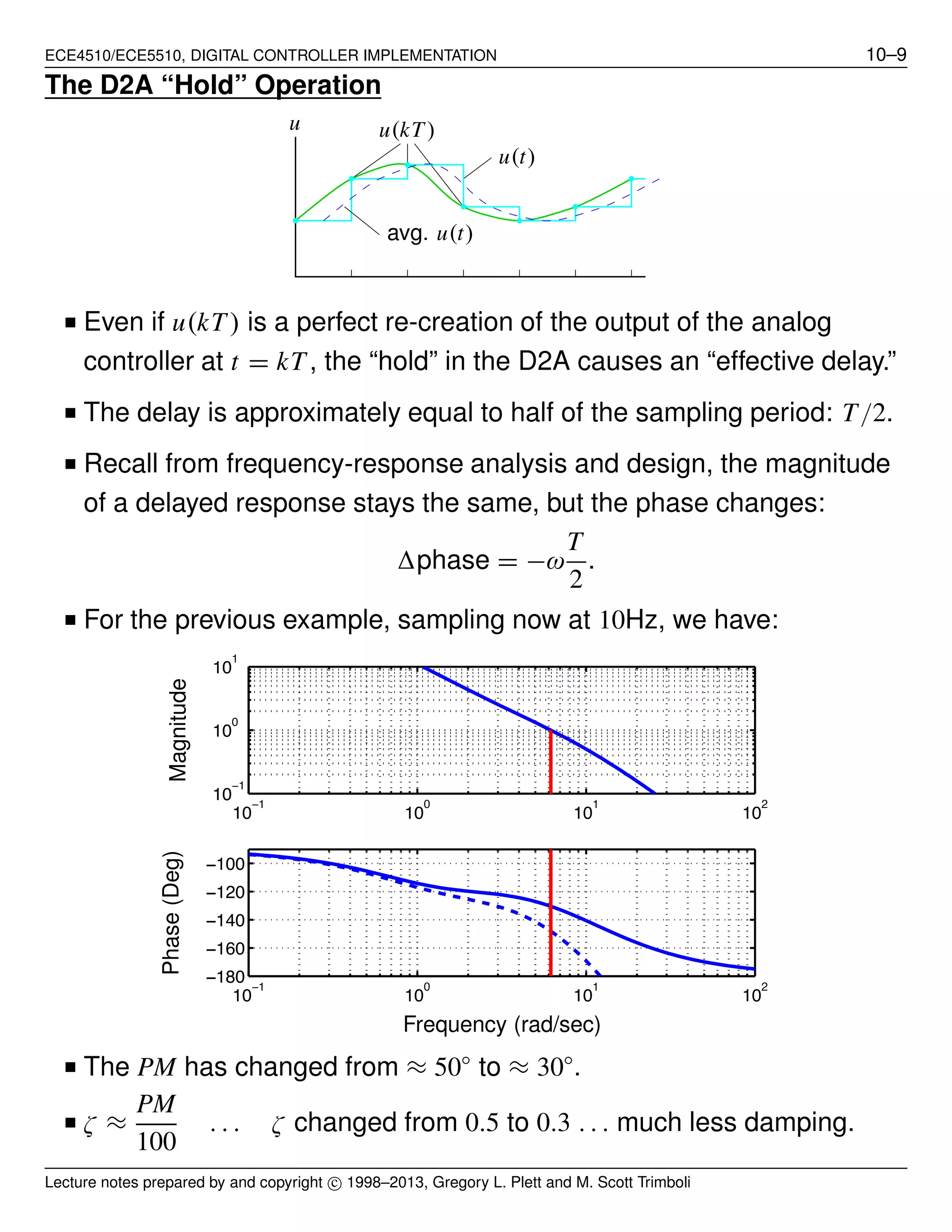
11. ECE4510/ECE5510, DIGITAL CONTROLLER IMPLEMENTATION 10–11
■ Gain is negative! We need to draw a 0◦
root locus, not the 180◦
locus
we are more familiar with.
■ Conclusion: Delay destabilizes the system.
PID Control via Emulation
P: u(t) = Ke(t)
I: u(t) =
t
0
K
TI
e(τ) dτ
D: u(t) = K TD ˙e(t)
⎫
⎪⎪⎪⎬
⎪⎪⎪⎭
PID: u(t) = K e(t) +
1
TI
t
0
e(τ) dτ + TD ˙e(t)
or, ˙u(t) = K ˙e(t) +
1
TI
e(t) + TD ¨e(t) .
■ Convert to discrete-time (use fwd. rule twice for ¨e(t)).
u[k] = u[k−1]+K 1 +
T
TI
+
TD
T
e[k] − 1 +
2TD
T
e[k − 1] +
TD
T
e[k − 2] .
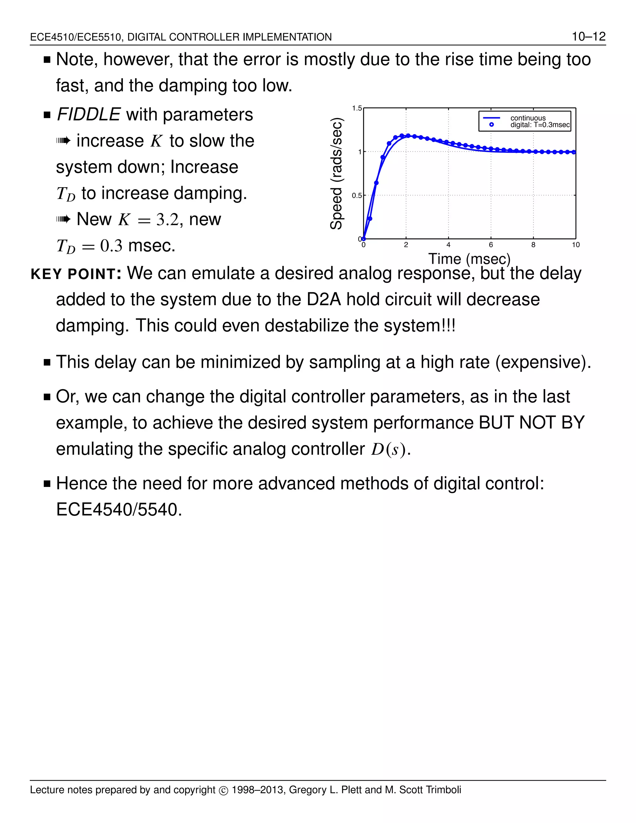
EXAMPLE:
G(s) =
360000
(s + 60)(s + 600)
K = 5, TD = 0.0008, TI = 0.003.
Bode plot of cts-time OL system D(s)G(s) with the above PID D(s)
shows that BW ≈ 1800 rad/sec, ≈ 320Hz.
10 × BW ➠ T = 0.3 msec.
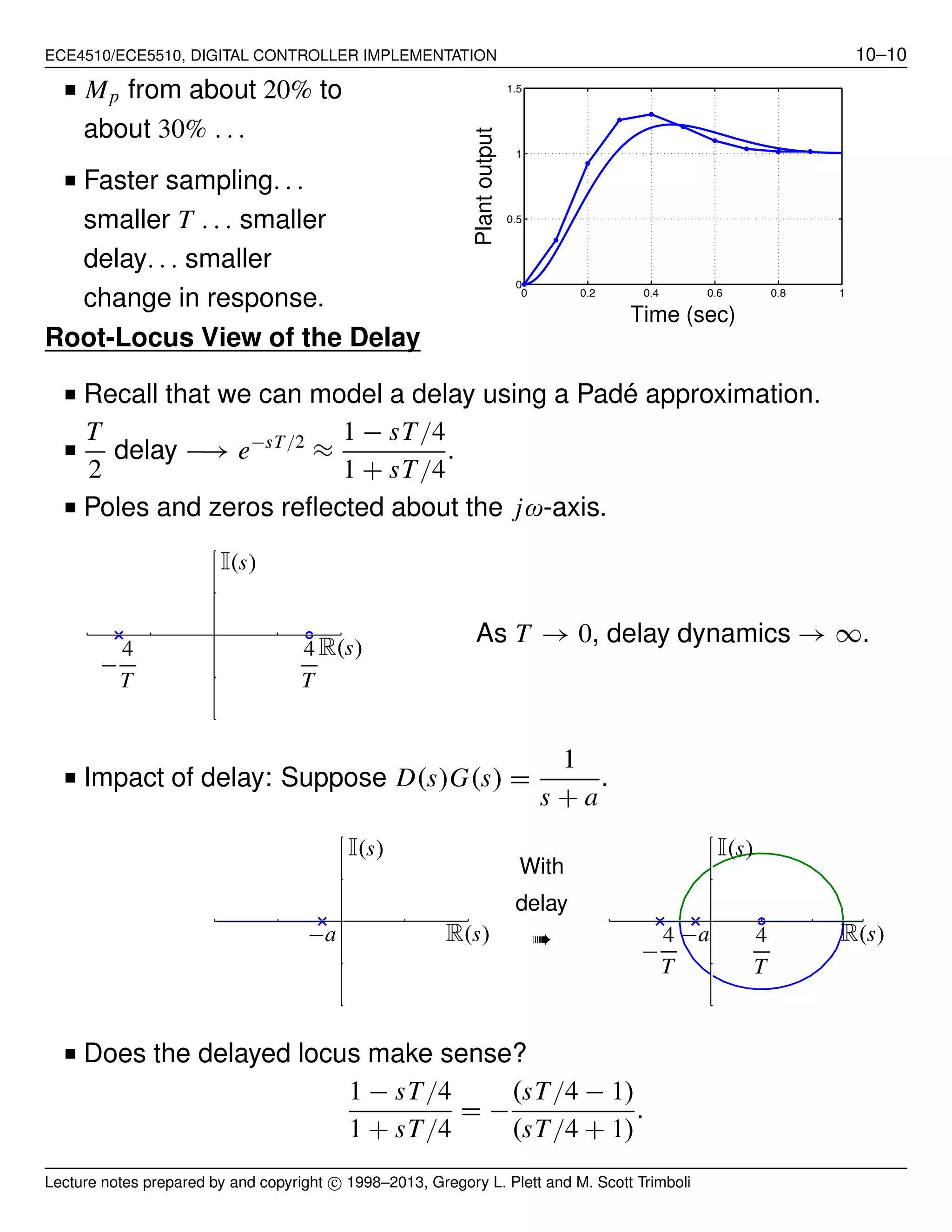
■ From above,
u[k] = u[k − 1] + 5 3.7667e[k] − 6.333e[k − 1] + 2.6667e[k − 2] .
■ Step response plotted to
the right.
■ Performance not great, so
tried again with T = 0.1
msec. Much better. 0 2 4 6 8 10
0
0.2
0.4
0.6
0.8
1
1.2
1.4
continuous
digital: T=0.3msec
digital: T=0.1msec
Time (msec)
Speed(rads/sec)
Lecture notes prepared by and copyright c⃝ 1998–2013, Gregory L. Plett and M. Scott Trimboli

12. ECE4510/ECE5510, DIGITAL CONTROLLER IMPLEMENTATION 10–12
■ Note, however, that the error is mostly due to the rise time being too
fast, and the damping too low.
■ FIDDLE with parameters
➠ increase K to slow the
system down; Increase
TD to increase damping.
➠ New K = 3.2, new
TD = 0.3 msec. 0 2 4 6 8 10
0
0.5
1
1.5
continuous
digital: T=0.3msec
Time (msec)
Speed(rads/sec)
KEY POINT: We can emulate a desired analog response, but the delay
added to the system due to the D2A hold circuit will decrease
damping. This could even destabilize the system!!!
■ This delay can be minimized by sampling at a high rate (expensive).
■ Or, we can change the digital controller parameters, as in the last
example, to achieve the desired system performance BUT NOT BY
emulating the specific analog controller D(s).
■ Hence the need for more advanced methods of digital control:
ECE4540/5540.
Lecture notes prepared by and copyright c⃝ 1998–2013, Gregory L. Plett and M. Scott Trimboli