Sorting

1. Week-4
Sorting

2. 2
Sorting
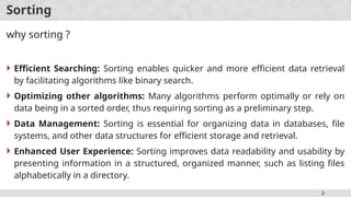
why sorting ?
 Efficient Searching: Sorting enables quicker and more efficient data retrieval
by facilitating algorithms like binary search.
 Optimizing other algorithms: Many algorithms perform optimally or rely on
data being in a sorted order, thus requiring sorting as a preliminary step.
 Data Management: Sorting is essential for organizing data in databases, file
systems, and other data structures for efficient storage and retrieval.
 Enhanced User Experience: Sorting improves data readability and usability by
presenting information in a structured, organized manner, such as listing files
alphabetically in a directory.

3. 3
Sorting
 Sorting
 Bubble sort
 Selection Sort
 Insertion Sort
 Merge Sort

4. 4
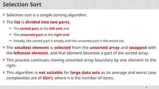
Selection Sort
 Selection sort is a simple sorting algorithm.
 The list is divided into two parts,
 The sorted part at the left end and
 The unsorted part at the right end.
 Initially, the sorted part is empty and the unsorted part is the entire list.
 The smallest element is selected from the unsorted array and swapped with
the leftmost element, and that element becomes a part of the sorted array.
 This process continues moving unsorted array boundary by one element to the
right.
 This algorithm is not suitable for large data sets as its average and worst case
complexities are of Ο(n2
), where n is the number of items.

5. 5
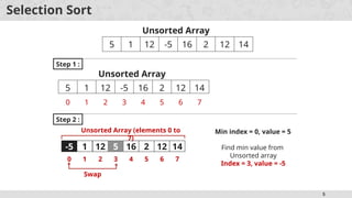
Selection Sort
5 1 12 -5 16 2 12 14
Unsorted Array
Step 1 :
5 1 12 -5 16 2 12 14
Unsorted Array
0 1 2 3 4 5 6 7
Step 2 :
Min index = 0, value = 5
5 1 12 -5 16 2 12 14
0 1 2 3 4 5 6 7
Find min value from
Unsorted array
Index = 3, value = -5
Unsorted Array (elements 0 to
7)
Swap
-5 5

6. 6
Selection Sort
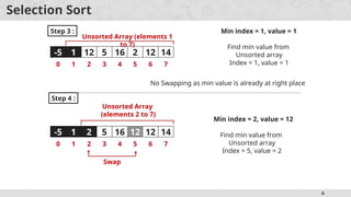
Step 3 :
-5 1 12 5 16 2 12 14
0 1 2 3 4 5 6 7
Unsorted Array (elements 1
to 7)
Min index = 1, value = 1
Find min value from
Unsorted array
Index = 1, value = 1
No Swapping as min value is already at right place
1
Step 4 :
-5 1 12 5 16 2 12 14
0 1 2 3 4 5 6 7
Unsorted Array
(elements 2 to 7)
Min index = 2, value = 12
Find min value from
Unsorted array
Index = 5, value = 2
Swap
2 12

7. 7
Selection Sort
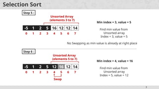
Step 5 :
-5 1 2 5 16 12 12 14
0 1 2 3 4 5 6 7
Min index = 3, value = 5
Find min value from
Unsorted array
Index = 3, value = 5
Step 6 :
-5 1 2 5 16 12 12 14
0 1 2 3 4 5 6 7
Min index = 4, value = 16
Find min value from
Unsorted array
Index = 5, value = 12
Swap
Unsorted Array
(elements 3 to 7)
No Swapping as min value is already at right place
5
Unsorted Array
(elements 5 to 7)
12 16

8. 8
Selection Sort
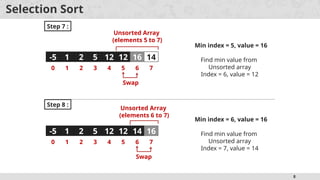
Step 7 :
-5 1 2 5 12 16 12 14
0 1 2 3 4 5 6 7
Min index = 5, value = 16
Find min value from
Unsorted array
Index = 6, value = 12
Swap
12 16
Unsorted Array
(elements 5 to 7)
-5 1 2 5 12 12 16 14
0 1 2 3 4 5 6 7
Min index = 6, value = 16
Find min value from
Unsorted array
Index = 7, value = 14
Swap
14 16
Unsorted Array
(elements 6 to 7)
Step 8 :

9. 9
SELECTION_SORT()
Steps to Implement Selection Sort
 for i 1 to n-1 do
←
 min i
←
 for j i+1 to n do
←
 { if A[j] < A[min] then{
 min j}}
←
 swap A[i], A[min]

10. 10
SELECTION_SORT()
The time complexity of Selection Sort:
Worst Case: O(n²)
Best Case: ?
Average Case: ?

11. 11
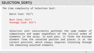
SELECTION_SORT()
The time complexity of Selection Sort:
Worst Case: O(n²)
Best Case: O(n²)
Average Case: O(n²)
Selection sort consistently performs the same number of
comparisons and swaps regardless of the initial order of
elements in the array. In each pass, it finds the minimum
element from the unsorted portion and places it at the
correct position, which always requires iterating through
the remaining unsorted elements.

12. 12
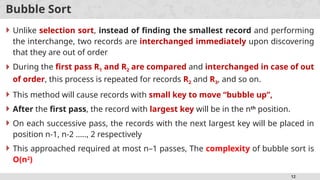
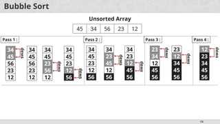
Bubble Sort
 Unlike selection sort, instead of finding the smallest record and performing
the interchange, two records are interchanged immediately upon discovering
that they are out of order
 During the first pass R1 and R2 are compared and interchanged in case of out
of order, this process is repeated for records R2 and R3, and so on.
 This method will cause records with small key to move “bubble up”,
 After the first pass, the record with largest key will be in the nth
position.
 On each successive pass, the records with the next largest key will be placed in
position n-1, n-2 ….., 2 respectively
 This approached required at most n–1 passes, The complexity of bubble sort is
O(n2
)

13. 13
Bubble Sort
45 34 56 23 12
Unsorted Array
Pass 1 :
45
34
56
23
12
34
45
56
23
12
34
45
56
23
12
34
45
23
56
12
34
45
swap
swap
23
56
swap
12
56
Pass 2 :
34
45
23
12
56
34
45
23
12
56
34
23
45
12
56
34
23
12
45
56
swap
23
45
swap
12
45
Pass 3 :
23
34
12
45
56
23
12
34
45
56
swap
23
34
swap
12
34
Pass 4 :
swap
12
23

14. 14
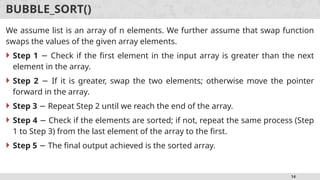
BUBBLE_SORT()
We assume list is an array of n elements. We further assume that swap function
swaps the values of the given array elements.
 Step 1 Check if the first element in the input array is greater than the next
−
element in the array.
 Step 2 If it is greater, swap the two elements; otherwise move the pointer
−
forward in the array.
 Step 3 Repeat Step 2 until we reach the end of the array.
−
 Step 4 Check if the elements are sorted; if not, repeat the same process (Step
−
1 to Step 3) from the last element of the array to the first.
 Step 5 The final output achieved is the sorted array.
−

15. 15
Procedure: BUBBLE_SORT ()
Pseudocode: Bubble-Sort(A)
for i ← 1 to less than n-1 do
for j ← 1 to less than n-i do
if A[j] > A[j+1] then
temp ← A[j]
A[j] ← A[j+1]
A[j+1] ← temp

16. 16
Bubble_SORT()
The time complexity of Bubble Sort:
Worst Case: O(n²)
Best Case: ?
Average Case: ?

17. 17
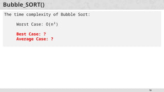
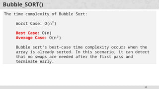
Bubble_SORT()
The time complexity of Bubble Sort:
Worst Case: O(n²)
Best Case: O(n)
Average Case: O(n²)
Bubble sort's best-case time complexity occurs when the
array is already sorted. In this scenario, it can detect
that no swaps are needed after the first pass and
terminate early.

18. 18
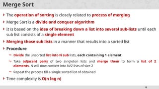
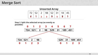
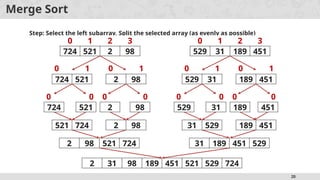
Merge Sort
 The operation of sorting is closely related to process of merging
 Merge Sort is a divide and conquer algorithm
 It is based on the idea of breaking down a list into several sub-lists until each
sub list consists of a single element
 Merging those sub lists in a manner that results into a sorted list
 Procedure
 Divide the unsorted list into N sub lists, each containing 1 element
 Take adjacent pairs of two singleton lists and merge them to form a list of 2
elements. N will now convert into N/2 lists of size 2
 Repeat the process till a single sorted list of obtained
 Time complexity is O(n log n)

19. 19
Merge Sort
72
4
52
1
2 98 52
9
31 18
9
45
1
Unsorted Array
0 1 2 3 4 5 6 7
724 521 2 98 529 31 189 451
0 1 2 3 4 5 6 7
Step 1: Split the selected array (as evenly as
possible)
724 521 2 98
0 1 2 3
529 31 189 451
0 1 2 3

20. 20
Merge Sort
Step: Select the left subarray, Split the selected array (as evenly as possible)
724 521 2 98
0 1 2 3
529 31 189 451
0 1 2 3
724 521
0 1
2 98
0 1
724
0
521
0
2
0
98
0
521 724 2 98
2 98 521 724
529 31
0 1
189 451
0 1
529
0
31
0
189
0
451
0
31 529 189 451
31 189 451 529
2 31 98 189 451 521 529 724

21. 21
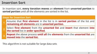
Insertion Sort
In insertion sort, every iteration moves an element from unsorted portion to
sorted portion until all the elements are sorted in the list.
Steps for Insertion Sort
1
Assume that first element in the list is in sorted portion of the list and
remaining all elements are in unsorted portion.
2
Select first element from the unsorted list and insert that element into
the sorted list in order specified.
3
Repeat the above process until all the elements from the unsorted list are
moved into the sorted list.
This algorithm is not suitable for large data sets

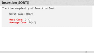
22. 22
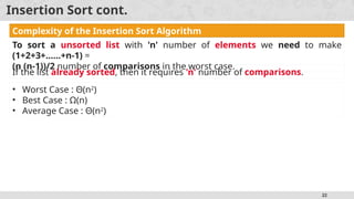
Insertion Sort cont.
Complexity of the Insertion Sort Algorithm
To sort a unsorted list with 'n' number of elements we need to make
(1+2+3+......+n-1) =
(n (n-1))/2 number of comparisons in the worst case.
If the list already sorted, then it requires 'n' number of comparisons.
• Worst Case : Θ(n2
)
• Best Case : Ω(n)
• Average Case : Θ(n2
)

23. 23
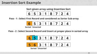
Insertion Sort Example
Sort given array using Insertion Sort
Pass - 1 : Select First Record and considered as Sorter Sub-array
5 3 1 8 7 2 4
6 5 3 1 8 7 2 4
6 5 3 1 8 7 2 4
6
Sorted Unsorted
Pass - 2 : Select Second Record and Insert at proper place in sorted array
5 6 3 1 8 7 2 4
Sorted Unsorted

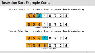
24. 24
Insertion Sort Example Cont.
Pass - 3 : Select Third record and Insert at proper place in sorted array
5 6 3 1 8 7 2 4
3 5 6 1 8 7 2 4
Sorted Unsorted
Pass - 4 : Select Forth record and Insert at proper place in sorted array
3 5 6 1 8 7 2 4
1 3 5 6 8 7 2 4
Sorted Unsorted

25. 25
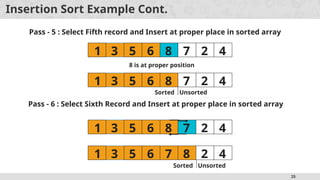
Insertion Sort Example Cont.
1 3 5 6 8 7 2 4
Pass - 5 : Select Fifth record and Insert at proper place in sorted array
1 3 5 6 8 7 2 4
8 is at proper position
Pass - 6 : Select Sixth Record and Insert at proper place in sorted array
1 3 5 6 8 7 2 4
1 3 5 6 7 8 2 4
Sorted Unsorted
Sorted Unsorted

26. 26
Insertion Sort Example Cont.
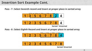
Pass - 7 : Select Seventh record and Insert at proper place in sorted array
1 2 3 5 6 7 8 4
Pass - 8 : Select Eighth Record and Insert at proper place in sorted array
Sorted Unsorted
1 3 5 6 7 8 2 4
1 2 3 5 6 7 8 4
1 2 3 5 6 7 8
4
Sorted Unsorted

27. 27
Insertion_SORT()
The time complexity of Insertion Sort:
Worst Case: O(n²)
Best Case: O(n)
Average Case: O(n²)